The Application of Tunable Magnetic Devices in Electrical Power Systems with Adaptive Features

Abstract

This work is devoted to possible implementation of tunable magnetic devices in electrical systems with adaptive properties. The basic idea, underlying operation of the presented magnetic device, depends on interaction of two (or more) magnetic fluxes in a quasi-linear range of ferromagnetic core characteristics. This is a new approach to the design of such magnetic elements; typically, saturation phenomenon of the ferromagnetic core of an inductor is used to change a value of its inductance. The good examples of adaptive electrical power systems can be devices for improving a quality of electrical energy. When used in compensators of reactive and a distortion power (or a reactive power only), tunable magnetic devices clearly offer wider possibilities for the compensation, compared to solutions, using compensators based on fixed magnetic elements. However, the application of the proposed tunable device in an adaptive compensator is only one example of its possible use in an electrical power area. In this work, the following issues are presented: exemplary solution of the adaptive passive compensator, basics of operation of tunable magnetic device, and test results of the experimental model of an electrical system with such a device.

1. Introduction

This work focuses on the idea of operation and possible implementation of tunable magnetic devices in electrical power systems with adaptive features. In the following text, this device is mostly referred to as the “tuned inductor” (TI). The basic idea underlying operation of the TI, depends on interaction of two magnetic fluxes in a quasi-linear range of ferromagnetic core characteristics, which is the new approach to the design of such magnetic devices. In contrast to this approach, typically, the effect of non-linearity (saturation) of a core of an inductor is used to change in value of its inductance.

The first group of adaptive systems which often needs change in its electrical characteristics are systems for improving the quality of electricity [1,2,3,4]. A further possible area of usage of the TI solutions is in static power electronics devices, formally known as flexible AC transmission systems (FACTS) [1,5,6], installed in AC grids. Such systems can increase the value of grid power transfer capability, stability, and controllability of grid operation, through series and shunt power compensation. The third area of possible TI applications concerns AC/DC, DC/AC, and DC/DC converters, which allow for shaping of the converter frequency characteristics [7,8,9,10]. However, Section 2 of this work focuses mainly on the possibility of application of the TI devices in the first group of power electrical systems mentioned above.

The negative effect of non-linear loads on the operation of a power grid, resulting in a lowering of the desired parameter values for the electrical energy [11], is a very well-documented phenomenon. In view of this, various types of compensators, mainly consisting of different types of power filters, are used in these electrical systems as preventive measures [1,12,13,14]. The main task of these devices is to match the shape of the current at its input to the shape of the current, drawn from the same grid node by other loads. As a result of the compensation process the current, flowing from the power line node to these loads, should have both a suitable shape and a correct phase relationship with the voltage waveform in the node. The details of the compensation process depend on the chosen compensator operation strategy, that can be related to a reactive power alone or to both a reactive and a distortion power [2,15,16,17]. However, presented in this work, the operation of an adaptive passive compensator, as a whole, is not related to any given power theory. In addition, the use of the tuned inductor in this power device is only an example of possible implementations of TIs in the field of electrical power area. In the other words, this work focuses rather on the idea of the TI operation and analysis of test results of the TI models, then on details of implementation of this device in a given electrical system.

The further part of the work consists of five sections, which include the following issues: the topology of the adaptive passive compensator, the basics of operation of the TI device, the design of the TI device, the results of testing the experimental model of electrical power systems with the TI device, and the conclusions.

2. Adaptive Passive Devices for Improving the Quality of Electricity

A fixed-parameter passive compensator is able to improve the power factor of a supply source only when its load also has fixed values of parameters. When these values vary, the effectiveness of operation of this type of compensator is lowered [1,3,13,18], meaning that an adaptive compensator is necessary instead. A compensator has adaptive features if it can be tuned to changes in both load power and power line characteristics. This can be carried out by switches or through the use of reactive elements with adjustable parameter values. Adaptive compensators can be based on reactive power compensators equipped with semi-controlled devices, typically thyristors, or on switching compensators, generally known as active power filters (APFs), in which different types of fully controlled devices (e.g., transistors) are used in the input/output power stage of the compensator. However, when the value of load power is very high, switching compensators is not usually sufficient.

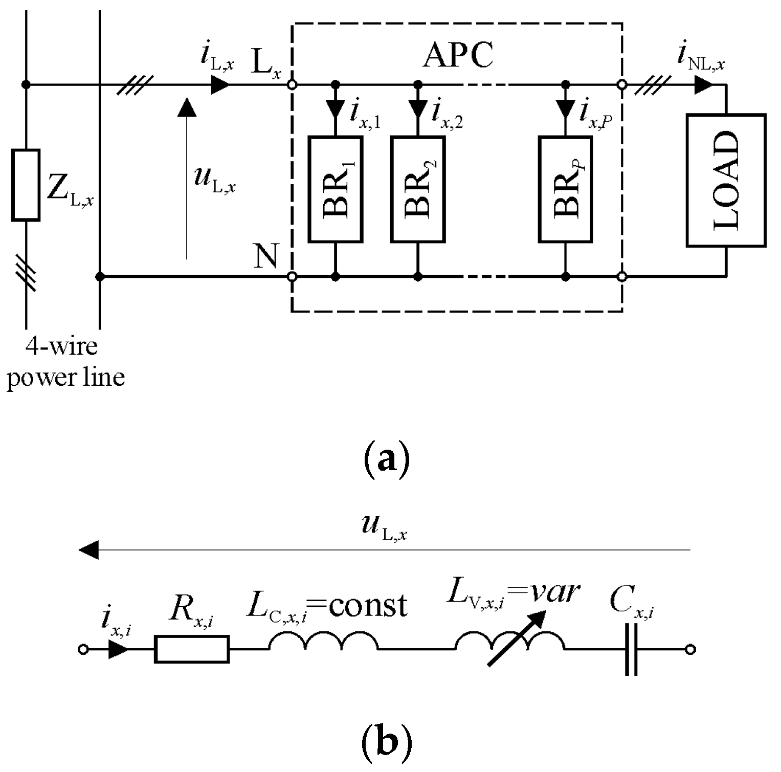
The generalized block diagram of the exemplary electrical system, consisting of an adaptive passive compensator (APC block) [1,3,13] is presented in Figure 1a.

The APC contains $P$ branches ($B{R}_i:i=1, 2, \dots , P$) that can be connected to each other in different ways, typically in parallel, see Figure 1a. An example of the topology of a single branch using the TI, is presented in Figure 1b. As a result of the operation of the tuned inductor, the impedance of the single branch can vary as follows:

$$\underset{\_}{Z_{x,i}}=\frac{\underset{\_}{U_{\mathrm{L},x}}}{\underset{\_}{I_{\mathrm{L},x,i}}}=R_{x,i}+\mathrm{j}{\omega }_{\mathrm{L}}(L_{\mathrm{C},x,i}+L_{\mathrm{V},x,i})-\frac{\mathrm{j}}{{\omega }_{\mathrm{L}}{C}_{x,i}},$$

(1)

where ${\omega }_{\mathrm{L}}$ is the fundamental frequency of the line voltage, $x$ is the phase number in a power line, and $i$ is the branch number in a given phase of the APC device.

As it follows from Equation (1), the presence of a tunable magnetic element in the branch of the APC device allows, for example, to change in the value of the branch self-resonance frequency. The maximum range of this change results from the relationship of $L_{\mathrm{V},x,i}$ = var and $L_{\mathrm{C},x,i}$ = const values. Taking into account the APC diagram, in the easiest mode of operation of this device, the $P$ factor can be interpreted as the maximum number of components of non-linear load current ($i_{\mathrm{NL},x}$), which are potentially possible to be compensated.

Nevertheless, it should be clearly stated that the APC is not, in formal terms, a fully passive system (as it follows from the diagram), since this compensator also uses different kinds of single power electronics switches or even complete power electronics switching converters. These devices are necessary to control the TIs, and their role in this type of power system is explained in detail in the next section.

3. Principle of Operation of a Tunable Inductive Device

From a formal side, the inductance of the coil is defined by the following formula [19]:

$$L=\frac{{\Phi }_{\mathrm{M}}}{i},$$

(2)

where ${\Phi }_{\mathrm{M}}$ is the total magnetic flux that is excited in the coil by the current ($i$) flowing in its winding. $i$ can also be interpreted as a sum of currents.

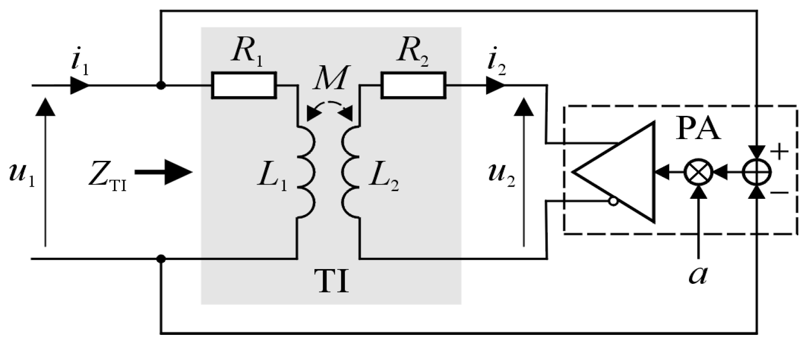
Based on Equation (2), for the implementation of a tunable magnetic device, the circuit with two magnetically coupled coils was used, see Figure 2.

This circuit consists of two main blocks; the first of these is the power transformer (denoted as the TI), which is equipped with the working air-gap in the core. The width of this air-gap influences the magnetic coupling factor ($k$) of these coils. The second block is the power amplifier (denoted as the PA), with scalable value of the gain factor ($a$). The PA device supplies the secondary winding of the TI. As a result of the operation of the PA block, the equivalent magnetic flux in the core can be amplified or weakened. As such, the equivalent impedance ($\underset{\_}{Z_{\mathrm{TI}}}=R_{\mathrm{TI}}+\mathrm{j}{X}_{\mathrm{TI}}$) of the circuit, when seen from the power source ($u_1$) side, can be changed too. In the other words, the value of $\underset{\_}{Z_{\mathrm{TI}}}$ depends on the value of the parameters of this circuit and, in particular, the actual value of $a$.

The value of $\underset{\_}{Z_{\mathrm{TI}}}$ was calculated based on an analysis of the basic properties of two magnetically coupled circuits [19]. The preliminary assumptions made here did not take into account the natural non-linearity of the ferromagnetic core of the transformer and the primary voltage excitation ($u_1$) was assumed to be sinusoidal.

In this case, the pair of equations, describing the voltages and currents relations in the circuit, is as follows:

$$\underset{\_}{U_1}=R_1\underset{\_}{I_1}+\mathrm{j}{X}_1\underset{\_}{I_1}+\mathrm{j}{X}_{\mathrm{M}}\underset{\_}{I_2},$$

(3)

$$\underset{\_}{U_2}=R_2\underset{\_}{I_2}+\mathrm{j}{X}_2\underset{\_}{I_2}+\mathrm{j}{X}_{\mathrm{M}}\underset{\_}{I_1},$$

(4)

where $X_1$, $X_2$, and $X_{\mathrm{M}}$ are the self- and mutual reactance of the circuit, respectively, and $R_1$ and $R_2$ are the resistances of the transformer windings.

Setting $\underset{\_}{U_2}=a\underset{\_}{U_1}$, the Equations (3) and (4) were transformed, to obtain the formula for the value of $\underset{\_}{Z_{\mathrm{TI}}}$:

$$\underset{\_}{Z_{\mathrm{TI}}}=\frac{\underset{\_}{U_1}}{\underset{\_}{I_1}}=\frac{R_1+\mathrm{j}{X}_1+\frac{X_{\mathrm{M}}^2}{R_2+\mathrm{j}{X}_2}}{1-a\frac{\mathrm{j}{X}_{\mathrm{M}}}{R_2+\mathrm{j}{X}_2}},$$

(5)

where:

$$X_{\mathrm{M}}=k\sqrt{X_1{X}_2} : 0\le k\le 1.$$

(6)

From Equations (5) and (6), the following expression was obtained, in which the value of $Z_{\mathrm{TI}}$ is dependent on the other parameters of this circuit, as follows:

$$\underset{\_}{Z_{\mathrm{TI}}}=\frac{R_1+\mathrm{j}{X}_1+k^2\frac{X_1{X}_2}{R_2+\mathrm{j}{X}_2}}{1-\mathrm{j}ak\frac{\sqrt{X_1{X}_2}}{R_2+\mathrm{j}{X}_2}}.$$

(7)

To extract the $X_{\mathrm{TI}}$ component of the impedance, both resistances were neglected. In this case, Equation (7) takes the form:

$$\underset{\_}{Z_{\mathrm{TI}}}=\mathrm{j}\frac{1-k^2}{1-ak\sqrt{\frac{X_1}{X_2}}}{X}_1.$$

(8)

Assuming the equality of values of both reactance (i.e., $X_1$ = $X_2$ = $X$) Equation (8) has the following final form:

$$\underset{\_}{Z_{\mathrm{TI}}}=\mathrm{j}\frac{1-k^2}{1-ak}X.$$

(9)

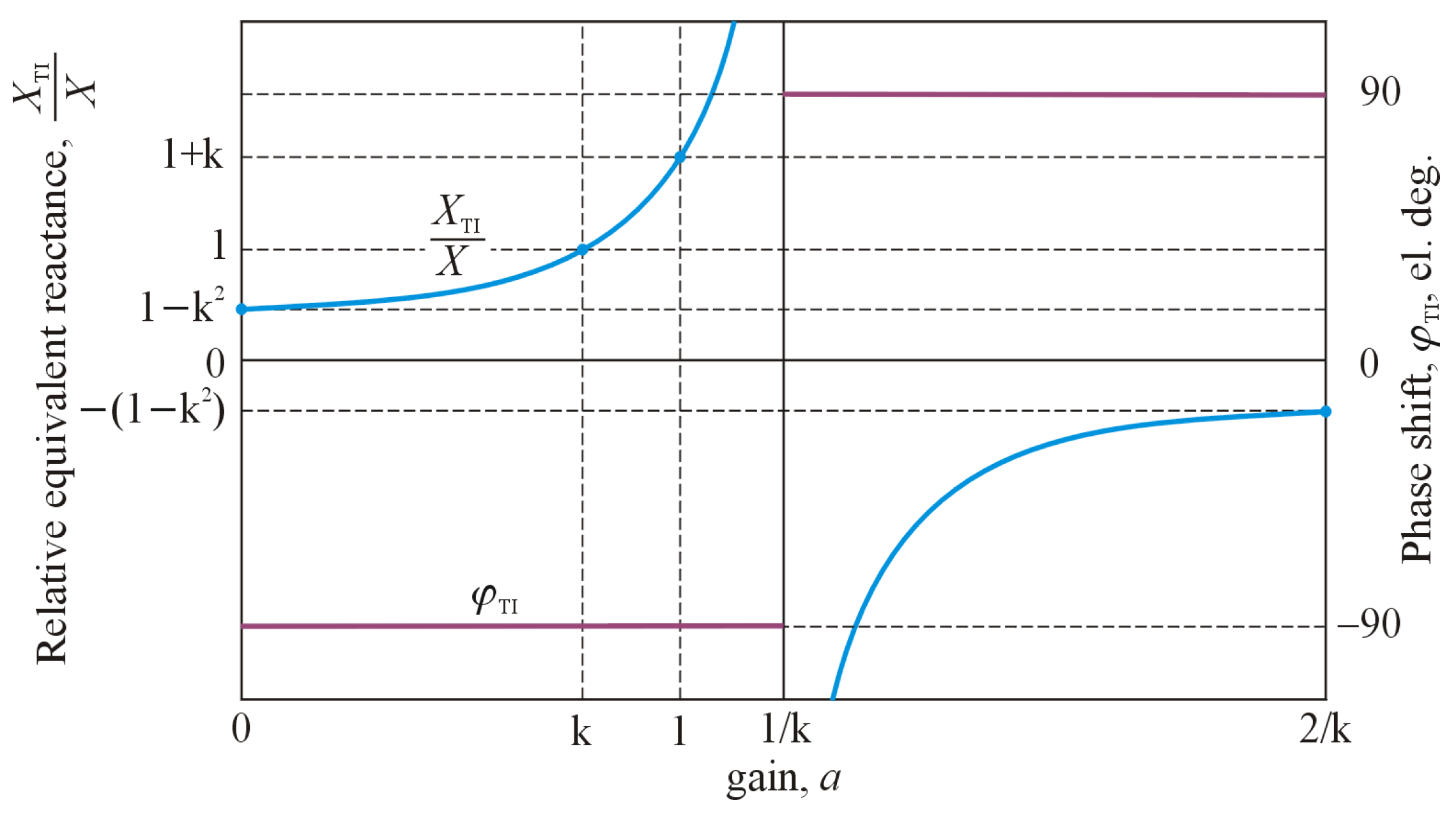
The plots of magnitude (as a value of $X_{\mathrm{TI}}$ related to $X$) and phase component (${\phi }_{\mathrm{TI}}$) of Equation (9), vs. $a$, while $k$ = const, are presented in Figure 3. In order to better visualize the details of the curves, the gain factor ($a$) variation was limited to the range of $<0, \frac{2}{k}>$. Values of reactance, for characteristic values of the gain factor are also shown at the magnitude curve as points. In relation to the right vertical axis of the chart, the abbreviation “el. deg.” denotes the “electrical degree”.

These curves show a singular point at $a$ = $\frac{1}{k}$. Thus, the value of $X_{\mathrm{TI}}$, in relation to the gain factor, lies within intervals given by the expression:

$$X_{\mathrm{TI}}\{\begin{array}{l}>0 : a<\frac{1}{k}\hfill \\ \to \pm \infty : a=\frac{1}{k}\hfill \\ <0 : a>\frac{1}{k}\hfill \end{array}.$$

(10)

From circuit theory [19], the interpretation of Equations (9) and (10) is that, depending on the value of the gain factor, the tunable magnetic device is equivalent to a variable inductance coil or a variable capacitance capacitor. However, in the latter case, it is obvious that it cannot form a capacitor as such, because it does not have the ability to store an electric charge. Nevertheless, in a real circuit, that description is given by Equations (5) and (7) and, due to the presence of the resistances, the aforementioned phase shift is different from ±90°. For simplicity, it was assumed again the equality of the reactance ($X_1$ = $X_2$ = $X$) and the resistances ($R_1$ = $R_2$ = $R$). In such a case the Equation (7) taken the form:

$$\underset{\_}{Z_{\mathrm{TI}}}=R\frac{1+{\left(\frac{X}{R}\right)}^2\left(k^2-1\right)+\mathrm{j}2\frac{X}{R}}{1+\mathrm{j}\left(1-ak\right)\frac{X}{R}}.$$

(11)

For easier interpretation of the circuit features, the time constant of the TI block (${\tau }_{\mathrm{TI}}$) was used in the next expression. As such, Equation (11) is now as follows:

$$\underset{\_}{Z_{\mathrm{TI}}}=R\frac{1+{\left(\omega {\tau }_{\mathrm{TI}}\right)}^2\left(k^2-1\right)+\mathrm{j}2\omega {\tau }_{\mathrm{TI}}}{1+\mathrm{j}\left(1-ak\right)\omega {\tau }_{\mathrm{TI}}} : {\tau }_{\mathrm{TI}}=\frac{L}{R}.$$

(12)

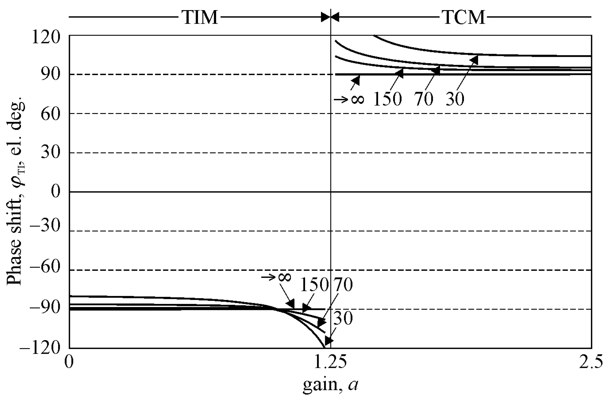
Figure 4 shows the plots of the phase shift based on Equation (12), vs. $a$, for $\omega {\tau }_{\mathrm{TI}}$ = const. The variation in the gain factor was limited to the range $<0, \frac{2}{k}>$ too.

A comparison with Figure 3 clearly shows phase errors, the values of which increase as the resistance increases which, in turn, results in a decrease in the value of $\omega {\tau }_{\mathrm{TI}}$. From the point of view of the properties of the TI block, its operation can be divided into two types based on the sign of the phase shift. If this sign is negative, the TI operates in the “tuned inductor mode” (TIM), while in the opposite case, it operates in the “tuned capacitor mode” (TCM), as illustrated in Figure 4.

4. Tuned Inductor’s Design

The aim of the research was to obtain all these technical details of the inductor–transformer, which are necessary for the design of its experimental prototype. At the initial stage of the project, the simulation studies of the TI three-dimensional field model (3-DFM) were conducted, using Maxwell Environment [20] together with the in-house optimization software [21]. This study showed that to achieve the assumed value for the inductance of the transformer, a sophisticated design of its magnetic circuit was necessary. As a result, a three-column magnetic core was chosen for the model of the transformer. Each of the columns was equipped with a working air-gap with a width equal to $g$. In the model, ferrite E-shapes, manufactured by MAGNETICS Inc. (catalogue number: OT49928EC), made of T-type ferrite material [22], were used. The model of the core was composed of four of shapes. It should be explained here why a ferrite core was chosen in the case of intended use of the tuned inductors at mains frequencies (i.e., related to value of 50 Hz). It was wanted simply to obtain a magnetic device with a wide pass-band property (at current research stage) so as to minimize the impact of undesirable effects, accompanying the operation of an inductor with a core made of transformer sheets. These effects are caused mainly by a very limited “pass-band” of magnetic material of this type; it is worth pointing out that the study of the tunable inductor, equipped with core based on the transformer sheets [23], was presented, in detail, in previous work [24].

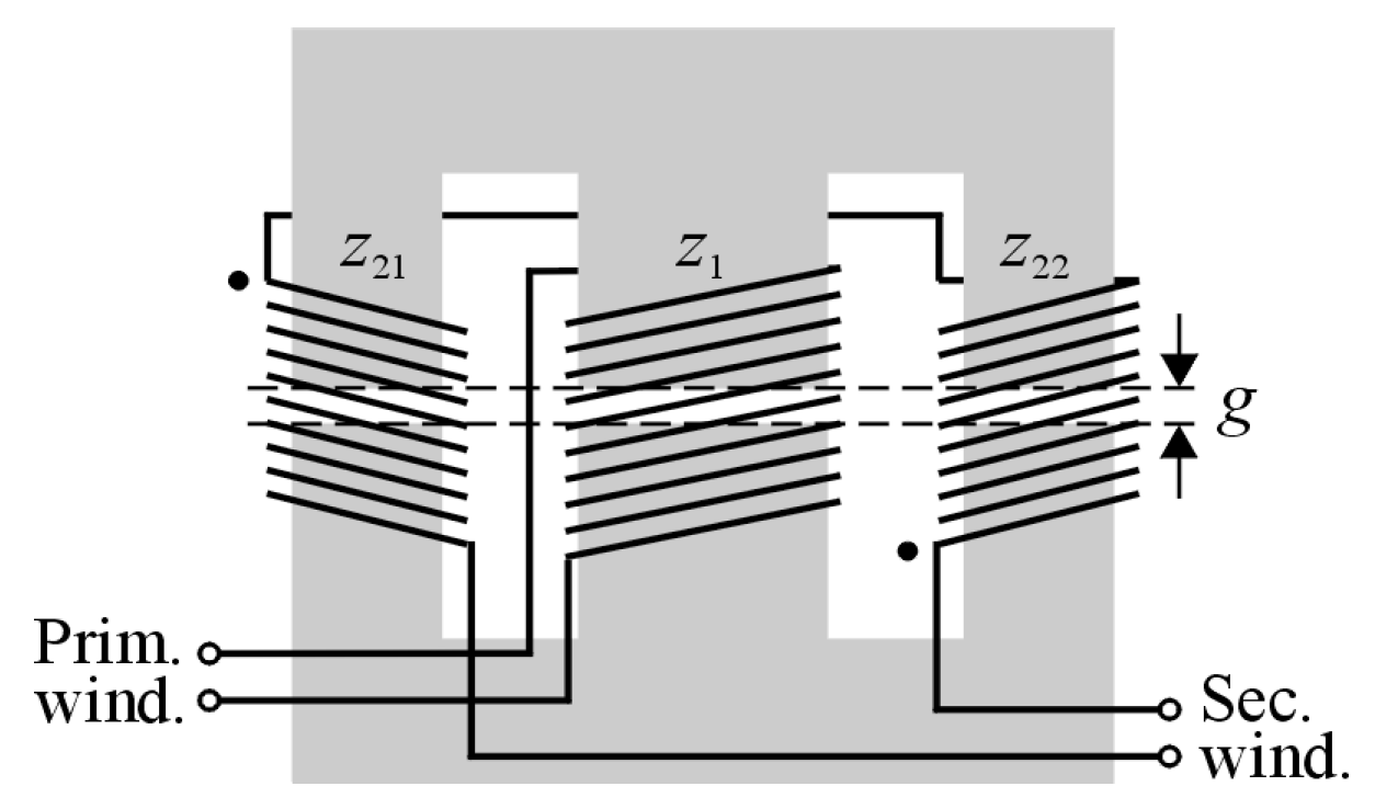
The primary coil of the transformer was wound on the central column of the core, while the secondary coil was divided into two equal parts and wound on both external columns. To simplify the whole modelling procedure, it was also assumed that the number of turns were equal for all of the coils, i.e., $z_1$ = $z_{21}$ = $z_{22}$, see Figure 5.

Respecting the potential fields of application of the TI device, reported in previous works [24,25], value of $X$, close to 4.50 mH, and value of $k$, close to 0.80, were assumed. These aforementioned works also present details of the entire inductor research procedure.

5. Laboratory Tests and Discussion

5.1. Tests of a Laboratory Prototype of the Adjustable Magnetic Device

In the power stage of the experimental model of the system with the TI, the P3-5-550MFE LABINVERTER [26] was applied. This power electronics device was designed especially for applications in advanced R&D power electronics systems. The control module of the LABINVERTER device comprised the ALS-G3-1369 evaluation board [26] with a 32-bit DSP (DSP—digital signal processor), Analog Devices Inc., Boston, MA, USA, type ADSP-21369 SHARC^®. This evaluation board is dedicated to such applications, which require both a CPU with high computation power and a PWM pattern with very high resolution, among others.

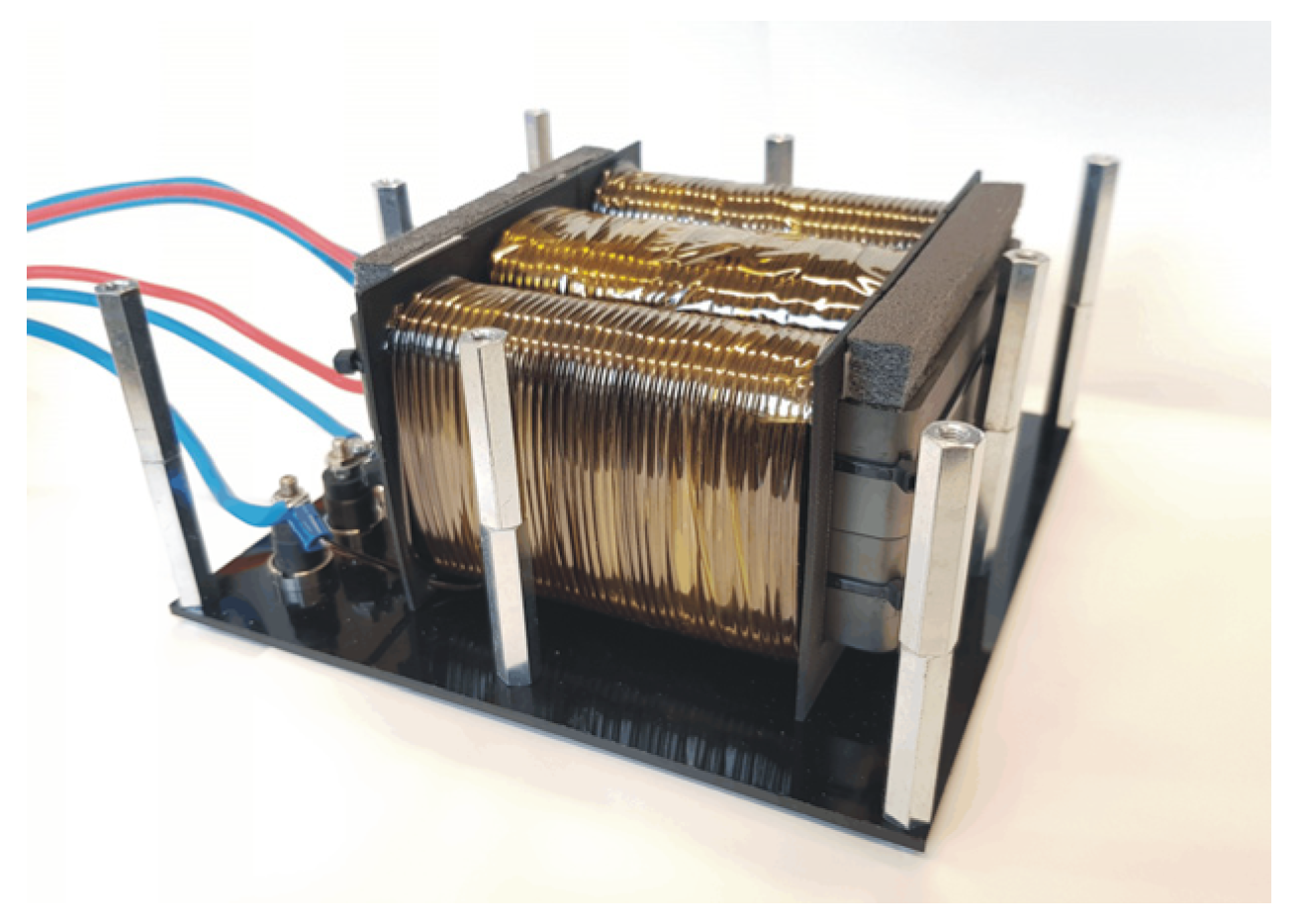
The general aim of this part of the investigation was to confirm the parameters for the experimental prototype of the TI in relation to its field model. A photograph of the experimental model of the TI is shown in Figure 6.

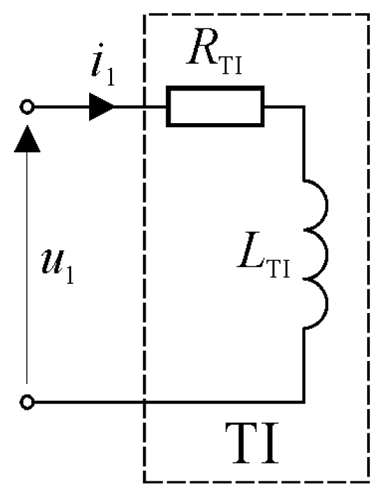
The methodology, used to calculate the inductance of the TI, was described in detail in a previous work [24]. As such, it is discussed here very briefly, only for the convenience of the reader. This methodology depended on the recording the voltage and current waveforms in the measurement circuit with the TI device, see Figure 7. These waveforms were then used as the basis for calculating the equivalent inductance of this device.

The general formula, respecting the voltage and current waveforms in the measurement circuit (in time-domain), is as follows:

$$u_1\left(t\right)=R_{\mathrm{TI}}{i}_1\left(t\right)+L_{\mathrm{TI}}\frac{\mathrm{d}{i}_1\left(t\right)}{\mathrm{d}t}.$$

(13)

For practical purposes, the resistive component of the circuit was neglected, and the supply voltage was assumed to be time’s rectangular function. As a result, the current waveform in this circuit will be time’s linear function, i.e., a first-order polynomial. Thus, the value of the inductance of the inductor can be calculated, using the following formula:

$$L_{\mathrm{TI}}=\frac{\mathsf{\Delta }{u}_1}{\mathsf{\Delta }{i}_1}\mathsf{\Delta }t,$$

(14)

where $\mathsf{\Delta }{u}_1$, $\mathsf{\Delta }{i}_1$, and $\mathsf{\Delta }t$ represent the changes in the voltage, current, and time, respectively.

The assumption that neglecting the resistances in the circuit does not result in a significant value of error in relation to the real inductance of the TI is true under the condition that the measurement time-interval ($\mathsf{\Delta }t$) is clearly shorter than the time-constant of the tested device, i.e.:

$$\mathsf{\Delta }t<<\frac{L_{\mathrm{TI}}}{R_{\mathrm{TI}}}.$$

(15)

This statement was confirmed experimentally based on a wide range of tests of numerous types of inductive devices; examples of such works are [24,25,27].

As a result of laboratory tests of the TI model, the following values were obtained for the parameters of this device:

• Number of turns: $z_1$ = $z_{21}$ = $z_{22}$ = 80;
• Air-gap width: $g$ = 2.0 mm;
• Inductance in relation to a quasi-linear range of the ferromagnetic core operation, while the secondary winding was open: $L_{\mathrm{TI},0}$ = 4.55 mH;
• Inductance while the secondary winding was short-circuited: $L_{\mathrm{TI},1}$ = 1.64 mH;
• Winding resistance: $R_1$ = 110 mΩ, $R_2$ = 220 mΩ.

Based on these assumptions for the TI model and from the results of laboratory investigations, the value of the magnetic coupling coefficient was calculated as $k$ = 0.80. The relationship between $L_{\mathrm{TI},0}$ and $L_{\mathrm{TI},1}$ is then equal to 2.8.

5.2. Tests of the Electrical System with a Tuned Inductor: Basic Configuration

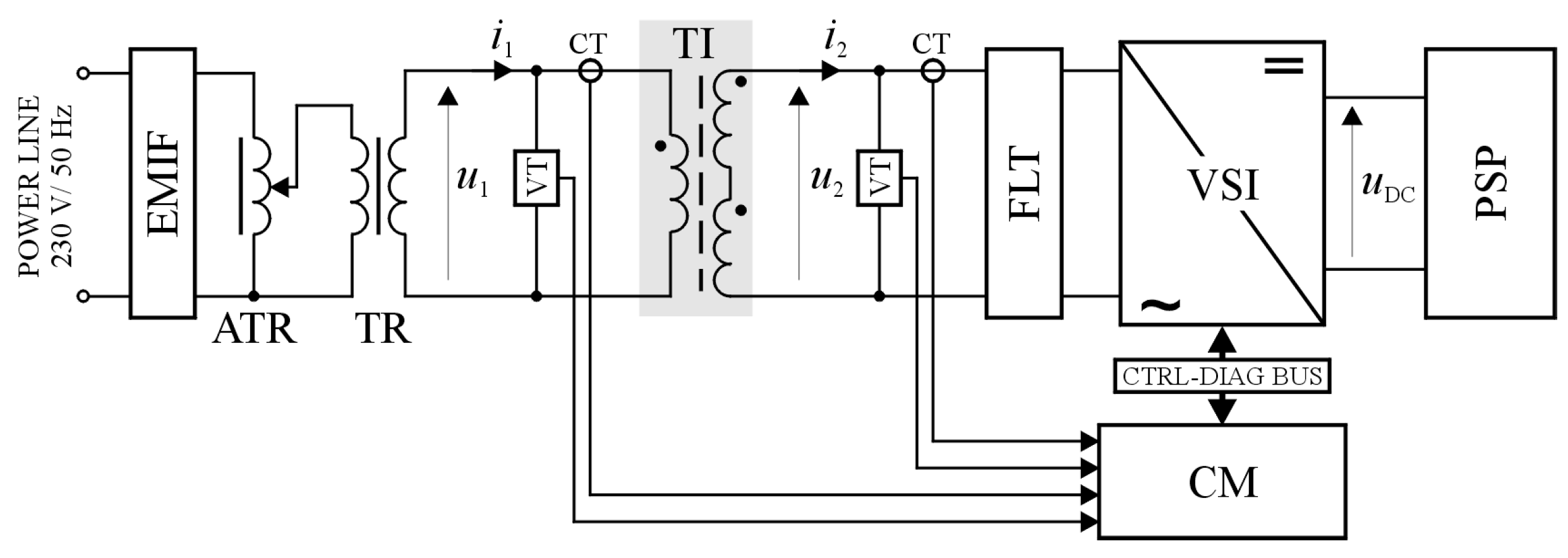
Figure 8 presents the block diagram of the laboratory system used to test the operation of the tuned magnetic device (TI) in the basic configuration. The aim of these tests was to confirm the assumed features of the TI as a tunable magnetic device, i.e., its ability to change in the equivalent inductance and more.

The measurement circuit contained the following main blocks and components:

• Power supply line and EMI filter (EMIF);
• Auto-transformer (ATR) as well as transformer (TR);
• Tested magnetic device (TI);
• H-bridge, voltage source inverter (VSI);
• LCL type filter (FLT), included at the output of the VSI;
• VSI control module (CM);
• Isolated current and voltage transducers (CT and VT, respectively);
• DC power supply with regulated the output voltage (PSP).

The CM and VSI was interconnected via a control and diagnostic bus (CTRL-DIAG BUS). As such, the VSI and FLT blocks made up the precision voltage controlled voltage source (VCVS), which powered the secondary windings of the TI device.

A wide range of tests were carried out on the system with the inductive device using the “hardware-in-the-loop” modelling. Most of the waveforms in the circuit were recorded using the PLOT function of DSP Emulator Software, Rev. 5.1.2, which is the part of VisualDSP++^® environment [28]. This function allows for easy graphic visualization of sets of data, stored as objects in the C/C++ language, such as numerical arrays, typically representing electrical (or other) waveforms. The C/C++ compiler is one of the main software components of VisualDSP++. During tests, the gain coefficient of the PA was varied within the interval of <0, 2.5> and the supply voltage ($u_1$) was set to 7 V RMS.

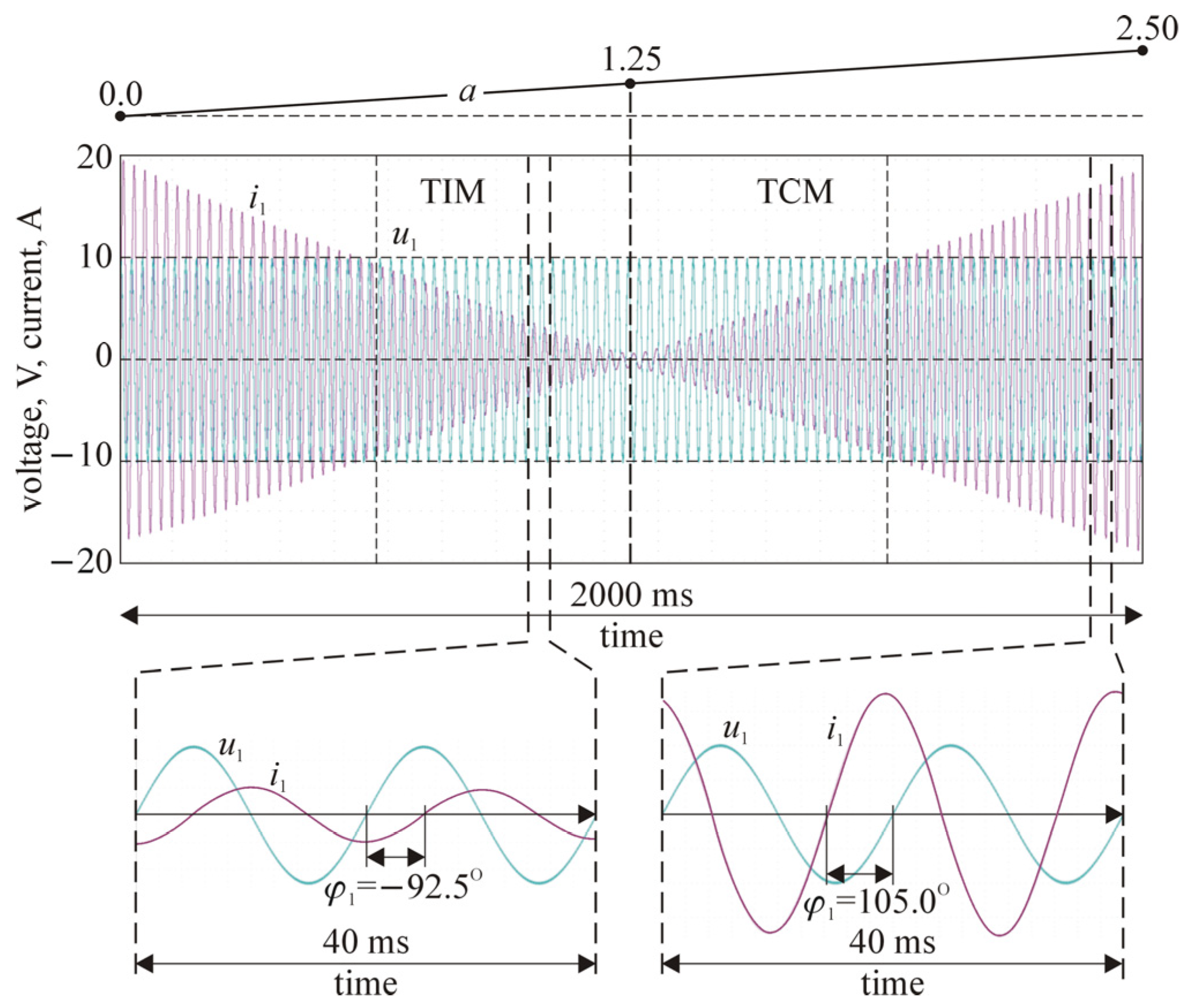
Figure 9 shows the most characteristic waveforms for the tested circuit, i.e., $u_1$ and $i_1$, as function of $a$, over time. The lower part of this figure shows details of the waveforms, including the phase relationship of $u_1$ and $i_1$. It can be seen clearly that after $a$ exceeds the value of $\raisebox{1ex}{$1$}\!\left/ \!\raisebox{-1ex}{$k$}\right.$, the circuit changes its character from an inductive to a capacitive one.

5.3. Tests of the Electrical System with a Tuned Inductor: Extended Configuration

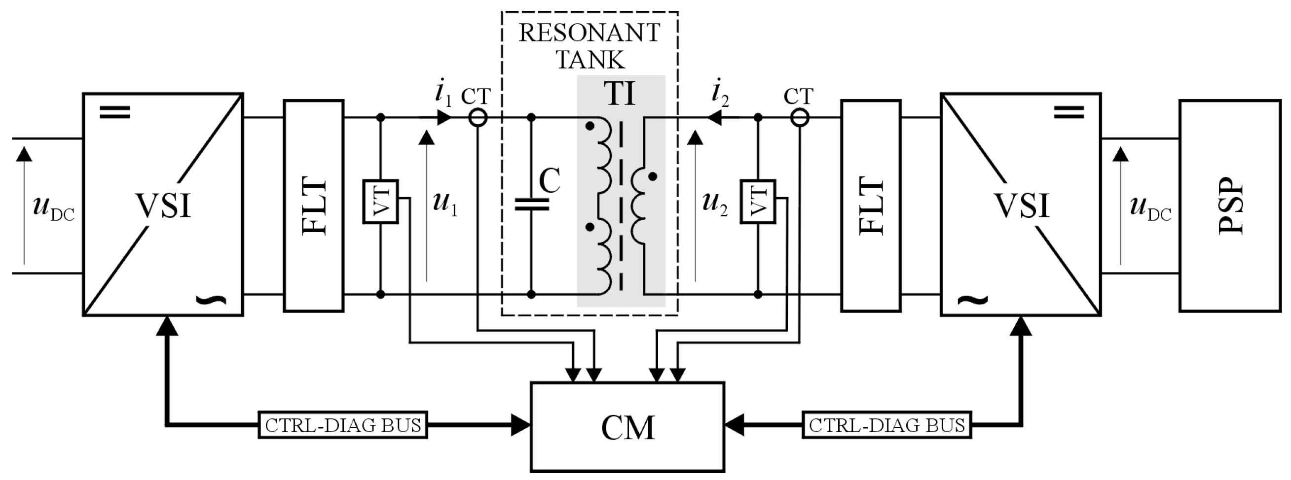
A block diagram of the laboratory system used to test the operation of the TI in the extended configuration is shown in Figure 10. The aim of these tests was to confirm the features of the TI device as a component of a tunable parallel resonant tank. This feature is related directly to its application in the APC devices.

The resonant tank (shown in the figure by the dashed line) was composed of TI and a capacitive element, which consisted of a set of high-quality polypropylene-film capacitors, with total value of C = 300 μF ± 1%. The gain coefficient of the PA was varied in the interval of <0, 1.25>. During these tests, the value of the primary voltage ($u_1$) was set to 10 V RMS, while its basic frequency was equal to 150 Hz (i.e., the third harmonics of the power line voltage). Thus, the system demanded implementation of the second VCVS block.

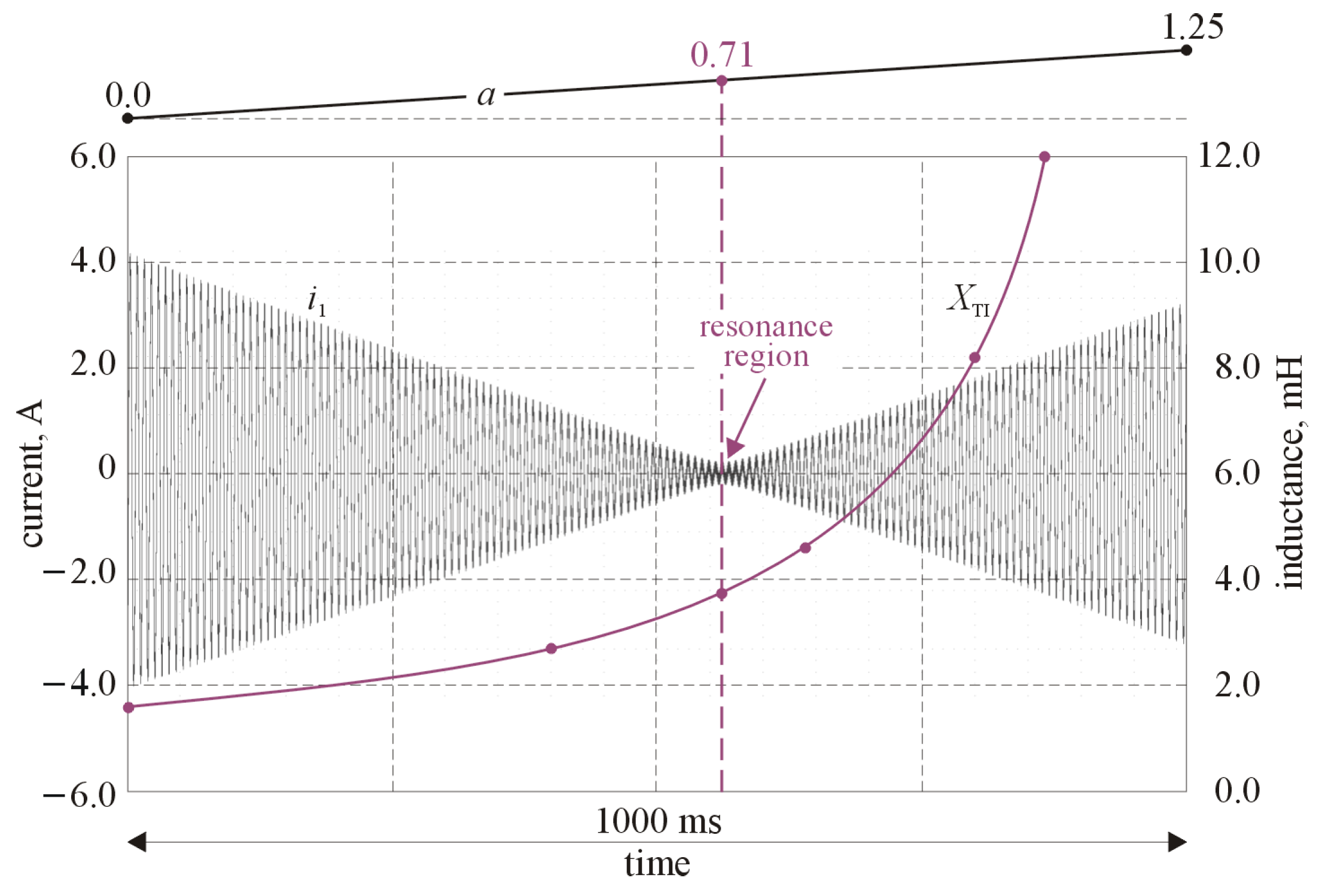
Figure 11 shows both the characteristic waveform for the circuit ($i_1$) and the plot of $a$ vs. time. A curve of the equivalent inductance vs. $a$ is also shown. From the figure, the moment at which parallel resonance occurs is clearly visible. This results from the given value of the equivalent inductance (reactance) of the TI, which is a function of $a$.

5.4. Discussion

The laboratory test results showed that, from the point of view of the relationship between the voltages and currents in the circuit, the inductive device presented here was able to operate in two modes, as either a tuned inductor or a tuned capacitor. However, the actual values of the equivalent reactance (the inductance or the “capacitance”) of TI were affected by an error of up to 15.0%, the value of which depended on the gain coefficient, which may result in a decrease in the equivalent reactance of the magnetic device. The error arose from factors such as:

• Presence of resistances in the tested circuit;
• Difference between the theoretical and the actual value of voltages in the primary and secondary circuit of the transformer (caused by, e.g., the gain error of the PA block);
• Presence of a ripple component in the transformer supply voltages that resulted from the pulse modulation (PWM) carrier component, as the PWM strategy was used to control the VSIs.

The phase shift of the primary current from the supply voltage was different from the desired value (i.e., −90° or +90°, depending on the mode of operation of this device), since the tested circuit contained, among others, the aforementioned TI winding resistances. The value of the phase error was in the range of 2.7–16.7%, depending on the actual value of the gain coefficient. Nevertheless, these tests proved that the proposed device can be an effective element of a tunable resonant tank, by determining its main property, i.e., the value of its self-resonance frequency. In this case, the error in the value of the resonance frequency, as a function of the gain factor, was no greater than 1% of its expected (theoretical) value. This value was within the range of error of the measuring instruments used. It should be noted that, in the simplified version, the tunable inductive device was also fully tested in a real electrical system with the DC power supply, equipped with the function of active compensation of both the reactive and the distortion power; see previous work [25].

6. Conclusions

This work presents the basics of operation and investigation results for model of electrical systems including a variable magnetic device. The operation of the device was based on the interaction between a pair of coupled fluxes but without relying on the natural non-linearity of the ferromagnetic circuit, as in most of the earlier studies, e.g., [1,19,29]. Instead, the interaction between two magnetic fluxes in the quasi-linear range of operation of the ferromagnetic core was exploited. The test results of experimental models confirmed the possibility of obtaining the desired reactance value in a smooth manner, as a result of control of the flux in the core of the inductor, with relative error of no more than 15%. In the author’s opinion, the above value can be considered satisfactory, taking into account the high complexity of both the magnetic circuit of the TI device and the entire electrical system with the TI. In addition, tests of a tunable resonant tank confirmed the utility of this device in a power electrical system. Taking into account the test results, it can be concluded that the operation of the magnetic element presented in this work was similar to that of a gyrator as an inverter of impedance [30]. Nevertheless, further investigations of the tuned inductor are needed to assess the impact of non-linearity of the real magnetic core and power loss in its operation.

Assumingly, it seems that the proposed device offers an attractive solution, particularly for electrical power systems with adaptive features, such as those used to improve the quality of electrical energy and for transmission this energy via power lines. However, these applications for the inductor also need further research using simulation and experimental models. Taking the above into account, the following are planned for the next phase of the research:

• Development of the experimental model of the adaptive passive compensator based on the current’s physical components (CPC) power theory [31], using TI devices;
• Extending and formalizing the description of the TI device as a power electronics gyrator.