On the Measure of the Heat Transfer Performance of RANS Turbulence Models in Single Round Jet Impingement

Abstract

The jet impingement phenomenon is one of the processes which can enhance heat transfer. Due to its complex nature, it has been the subject of many experimental and numerical analyses in which researchers have tried to quantify and qualitatively describe it. However, the lack of crucial information regarding procedures, accuracy, geometry settings, boundary conditions, etc. makes it challenging to compare the results, validate turbulence models, and reproduce data. In this publication, the authors show a consistent and systematic numerical analysis of round and turbulent jet impingement based on RANS turbulence models. The results have been calculated for various geometrical configurations, Reynolds number values, and turbulence models, and compared with experimental and numerical data available in the literature to show their similarities and differences. It led to unique data collection, which was used in the novel quantitative analysis and helped lead to proposing the measure of the heat transfer performance of a particular turbulence model. Such a measure has not been reported so far. The measure exhibited that no turbulence model is suitable for all analyzed parameters. Quantitative comparisons enable recommendations of turbulence models for analyzed cases which have the potential to accelerate the design process of devices and could be a source of suggestions for other researchers.

1. Introduction

Experimental studies of complex physical phenomena remain a challenge. They require much work, time, and money, and there is not a 100% certainty of success. A similarly or even more challenging task is numerical modeling, especially in the case of heat and momentum transfer. An example of such a complex phenomenon is jet impingement turbulent heat transfer. Jet impingement represents the stream of fluid discharged from the nozzle or orifice hitting the opposite wall. The most frequent turbulent jet goes through the stagnation region, changing direction, laminarizing, and then developing into a turbulent wall jet. Such changes in flow character involve strong gradients, which can be difficult to ‘catch’ because they depend on various parameters. The common problem of both experimental and numerical approaches is the lack of crucial information like configuration or geometrical setup details, data referring to the inlet conditions, boundary conditions, details of turbulence modeling, etc. One of the weak points of the research is repeatability. Therefore, without all the mentioned critical information, it is impossible to compare research work with the results of other research groups. It is also difficult to draw general conclusions about modeling the jet impingement phenomenon, synthesizing the available knowledge, and finding the reasons for the result discrepancies.

The experimental studies available in the literature have been conducted for many different geometrical configurations (distance to impingement plate and diameter ratio H/D) and values of Reynolds numbers; only a few of them corresponding to the selection in the presented numerical investigations were reported: H/D = 1, Re = 10,000–30,000 [1,2,3]; H/D = 2, Re = 10,000–30,000 [3,4,5,6,7,8,9]; H/D = 4, Re = 10,000–30,000 [2,3,4,6]; H/D = 6, Re = 10,000–30,000 [1,3,4,6,7,8,9,10,11]. A brief overview of the selected experimental investigations together with their achievements can be found in Table 1. The literature’s survey of the numerical investigations of the turbulence jet impingement phenomenon shows many studies, geometrical configurations, and flow conditions. A brief overview of the numerical investigations can be found in Table 2.

Table 1. A brief overview of the selected experimental investigations.

	H/D*	Re*	Scope and Some Key Findings
Colucci et al. [1]	1 6	10,000 20,000 30,000 20,000 30,000	Analysis of influence of nozzle geometry (orifice and two hyperbolic nozzles). The hyperbolic nozzle is better than the orifice for H/D < 1 and Re > 30,000; The local Nusselt number values depended strongly on the Reynolds number and H/D; For larger H/D (=6.0), the local Nusselt number was independent of the nozzle geometry; The effect of the confinement on the local Nusselt number increases with decreasing H/D.
Gulati et al. [2]	1 4	10,000	Analysis of the nozzle shape influence (circular, square, rectangular). An increase in the Reynolds number causes an increase in the heat transfer rate for circular and noncircular jets; The average Nusselt number was almost the same for all tested nozzle configurations; The pressure loss coefficient was the lowest for the circular jet and the highest for the rectangular one.
Katti et al. [3]	1 2 4 6	20,000 23,000	Experimental investigation and theoretical analysis of local heat transfer characteristics, and development of semiempirical correlations. Three regions were identified (stagnation, transition, and wall jet); An increase in the Reynolds number causes an increase in the heat transfer; The Nusselt number at the stagnation point increases with an increase in H/D from 1 to 6 (for constant Re); The Nusselt number at the stagnation point increases with a decrease in H/D below 1.
Lee et al. [4]	2 4 6	10,000 20,000 30,000	Investigation of local heat transfer characteristics in a stagnation region. Construction of heat transfer data benchmark. Proposal of the Nusselt number correlation. For small values of H/D (=2), the local Nusselt number distribution has two distinct maxima; The first maximum is related to the accelerated radial flow at the edge location of the nozzle, and the second maximum is due to the transition from laminar to a turbulent boundary layer; The locations of maxima move outward with increasing Reynolds numbers; For high values of H/D (>6), the local Nusselt number decreases monotonically with the radial distance; The Reynolds number dependence is enhanced with increasing H/D as a result of the increase in the centerline turbulence intensity of the jet.
Petera et al. [5]	2	23,000	Analysis of influence of the heat flux oscillations on the heat transfer process. Comparison between the experimental and CFD results. The best agreement was provided by the k-ω Intermittency Transition turbulence model; The second-order closure Reynolds Stress models with the implementation of the explicit algebraic model for the anisotropic turbulent heat flux obtained the best possible agreement with experimental data.
Gao et al. [6]	2 4 6	23,000	Study of heat transfer enhancement caused by the array of triangular tabs located at the turbulent jets’ exits. The addition of the tabs at the jet exits had a significant effect on the heat transfer produced by the impinging jet, particularly in the impingement region; For a small value of H/D (=2), the impinging jet produces a series of distinct regions of significant heat transfer enhancement surrounding the impingement region; For a higher value of H/D (=4 and =6), the heat transfer enhancement became more uniform; Tabs significantly increased the turbulent mixing and played an essential role in determining heat transfer enhancement for larger values of H/D; The turbulent mixing also reduced the development length of the jet.
Yan et al. [7]	2 6	23,000	Investigation of the local heat transfer coefficient for jet impinging on a flat plate. For a small value of H/D (=2), the heat transfer in the stagnation region is proportional to Re0.5 and in the wall jet region to Re0.7; For a large value of H/D (=6), the Reynolds number dependence in the wall jet region is unchanged, but in the stagnation region it is stronger, at Re0.56.
Baughn et al. [8]	2 6	23,300	Experimental study of jet impingement heat transfer. Influence of the entrainment effect. The effectiveness is independent of the Reynolds number and the jet temperature.
Baughn et al. [9]	2 6	23,750	Experimental analysis using a fully developed jet and well-controlled thermal boundary conditions. For H/D = 2, the maximum heat transfer is at the stagnation point, then has a minimum at x/D = ~1.3 and another maximum at x/D = ~1.8; The maximum stagnation point heat transfer occurs at H/D = 6.
Lytle et al. [10]	6	23,000	Local heat transfer characteristics at H/D < 1. Presentation of the Nusselt number correlation. With a decreasing value of H/D, both mean velocity and RMS turbulence fluctuations increase; For H/D < 0.25, heat transfer enhancement was observed due to the global continuity-forced acceleration of the fluid, as well as a significant increase in the turbulence level; The stagnation point heat transfer coefficients increase significantly with decreasing values of H/D.
Lee et al. [11]	6	23,000	Analysis of an influence of the diameter of the nozzle on heat transfer. The potential core length increases with an increasing nozzle diameter; The jet momentum and turbulence intensity increase with a larger nozzle diameter, which results in heat transfer enhancement at the stagnation point; For Re = 23,000 and all diameters of the nozzles, the maximum Nusselt number at the stagnation point occurs at H/D = 7. The intensity of the turbulence reaches roughly a maximum value in that region; The local Nusselt number increases with the increasing nozzle diameter in the stagnation region; There is no effect of the diameter of the nozzle on the local Nusselt number in the wall jet region (x/D > 0.5). Jet flow characteristics are almost lost in the redevelopment of the boundary condition layer.

The H/D* and Re* list is narrowed down to values used as a reference.

Table 2. Overview of numerical investigations.

	Jet Type	Nozzle Shape	Geometry	H/D	Re	Models
Seyedein et al. [12]	confined	slot	flat	2.5–7.5	5000–20,000	k-ε model family
Behnia et al. [13]	confined unconfined	round	flat (normal and inclined)	6	23,000	$\overline{v^2}\text{-}f$
Heyerichs et al. [14]	confined	slot	flat	2.6	10,000	k-ε and k-ω model family
Behnia et al. [15]	confined unconfined	round	flat, pedestal	0.1–6	23,000	$\overline{v^2}\text{-}f$
Kura et al. [16]	confined	round	flat	2	23,000	ζ-f
Jensen et al. [17]	unconfined	round	flat	2	1.1·105–6.6·105	$\overline{v^2}\text{-}f$ and k-ε model family
Huang et al. [18]	confined	slot	flat	4, 9.2		k-ω SST, Kato–Launder, Intermittency transition
Granados-Ortiz et al. [19]	unconfined	round	flat	5	23,000	k-ω SST, Kato–Launder, Transition SST
Wienand et al. [20]	unconfined	round	flat	2, 6, 10, 14	23,000	k-ω SST, Kato–Launder
Simionescu et al. [21]	unconfined	slot	flat	2–10	2000–10,000	k-ε and k-ω model family
Caggese et al. [22]	confined	round	flat	0.5, 1.0, 1.5	16,500–41,800	k-ω SST
Chen et al. [23]	confined	round	flat	2.5	~1.4·105–2.6·105	k-ω SST
Petera [24]	unconfined	round	flat	2, 6	23,000	k-ω SST, RSM, Intermittency transition, Transition SST, k-kl-ω
Hofmann et al. [25]	unconfined	round	flat	2.5, 10	34,000, 124,000	k-ε and k-ω model family, RSM
Sagot et al. [26]	unconfined	round	flat	2–6	10,000–30,000	k-ε and k-ω model family
Ortega-Casanova et al. [27]	unconfined	round	flat, surface with bumps	2	23,000	k-ω model family
Zhou et al. [28]	unconfined	round	flat	2	4000–12,000	$\overline{v^2}\text{-}f$, k-ε and k-ω model family, RSM
Buchlin [29]	unconfined	round	flat	1	60,000	k-ε RNG
Isman et al. [30]	confined	slot	flat	4–10	4000–12,000	k-ε model family
Nabadavis et al. [31]	unconfined	round	flat	3–30	20,000–51,000	k-ε model family
Sharif et al. [32]	confined	slot	flat, concave	2.6, 6	10,200, 11,000	k-ε model family, k-ω SST, RSM
Kura et al. [33]	confined	round	flat, concave, convex	2	23,000	$\overline{v^2}\text{-}f$, k-ε model family, k-ω SST
Kura et al. [34]	confined	round	flat	2	23,000	$\overline{v^2}\text{-}f,$ ζ-f, k-ε model family
Kura et al. [35]	confined	round	flat, concave, convex	2	23,000	$\overline{v^2}\text{-}f$, ζ-f
Aillaud et al. [36]	unconfined	round	flat	2	23,000	LES
Dutta et al. [37]	confined	slot	flat	4	20,000	LES
Hadžiabdić et al. [38]	unconfined	round	flat	2	20,000	LES
Dairay et al. [39]	confined	round	flat	2	10,000	LES
Uddin et al. [40]	confined	round	flat	2	13,000, 23,000	LES
Dairay et al. [41]	confined	round	flat	2	10,000	DNS

The information included in the table refers mostly to the geometry configurations, hydrodynamics conditions, and applied turbulence models. The researchers directly considered various parameters, modeling approaches to the Nusselt number distribution such as near wall treatment in RANS models [12,13,14], domain confinement [13,15], inlet velocity profiles [13,15,16], inlet turbulence intensity [15,17], the influence of the turbulent kinetic energy production limiter Kato–Launder [5,18,19,20], RANS turbulence models k-ω family [5,14,18,20,21,22,23,24,25,26,27,28], k-ε model family [12,13,14,17,21,25,26,28,29,30,31,32], Reynolds Stress Model [24,28,32], $\overline{v^2}\text{-}f$ [13,15,17,28,33,34,35], and ζ-f [16,34,35]. Few numerical investigations have been conducted for LES calculations to explain the second maksimum of the Nusselt number [36,37,38,39,40]. One publication with DNS results is also available in the literature [41].

As can be seen, much work was already involved in analyzing single jet impingement. However, it is not easy to compare the results. The researchers applied more and more advanced numerical methods to get close to the experimental results, but one of the reasons for the observed discrepancies may be the unknown or imprecise definition of the accuracy of the boundary conditions. Therefore, general conclusions are not drawn, and researchers focus on particular problems’ solutions.

Jambunathan et al.’s [42] work shows and attempts to explain scattering in the experimental results under the influence of the geometry or confinement. This example shows that the discrepancies in the empirical studies are well known in the jet impingement community. The lack of detailed information on various parameters in experimental studies, such as the inlet velocity profile, the intensity of the turbulence, or even the geometric dimensions of the nozzle, leads to problems when using it as a benchmark for numerical investigations [13,43]. Kura et al. [16] reveal that the problem with the shortage of information in research publications goes beyond experimental studies and also occurs in numerical investigations. Without information about the flow conditions, turbulence modeling, full geometry definition, research, and the results, comparisons are very difficult or even impossible to make. Therefore, there is a need for such a detailed description.

The presented numerical investigations of the single round turbulent jet impingement phenomenon focused on RANS turbulence modeling because of its low computation cost compared with other approaches. Furthermore, due to the significant fragmentation of numerical investigations in the literature, a consistent numerical study is introduced for four different geometrical configurations, four Reynolds numbers, five different RANS turbulence models, and a complete numerical setup. Moreover, the results are included in a unique data collection available to everybody. The results are then compared with experimental and numerical studies available in the literature. The method of comparison is proposed by the authors, because such a method has not been found in the literature so far. The measure for the comparison between the results obtained from various turbulence models was proposed and gave a very good tool to quantify the level of agreement between them.

2. Numerical Model

Assuming that the fluid was Newtonian, incompressible, and without additional sources of mass, momentum, and energy, the mathematical model based on the RANS approach consisted of three stationary transport equations: mass, momentum, and energy, defined as follows:

$$\frac{\partial U_i}{\partial x_i}=0$$

(1)

$$\rho \frac{\partial }{\partial x_i}\left(U_i{U}_j\right)=-\frac{\partial P}{\partial x_i}+\frac{\partial }{\partial x_i}\left(2\mu S_{ij}-\rho \overline{u_i{u}_j}\right)$$

(2)

$$\frac{\partial }{\partial x_i}\left(U_i\Theta \right)=\frac{\partial }{\partial x_i}\left(a\frac{\partial \Theta }{\partial x_i}-\overline{u_i\theta }\right)$$

(3)

where: $U_{i,j}$ are the average velocity components, m/s; $\rho$ is the density, kg/m³; $P$ is the average pressure, Pa; $\mu$ is the dynamic viscosity, Pa·s; $S_{i,j}$ is the strain rate tensor, 1/s; $\overline{u_i{u}_j}$ is the Reynolds stress term, m²/s²; $\Theta$ is the average temperature, K; $a$ is the thermal diffusivity, m²/s and $\overline{u_j\theta }$ is the turbulent heat flux, K·m/s.

When analyzing a turbulence phenomenon, it is necessary to incorporate the additional equations of the turbulence models in the model, such as k, ε, ω, intermittency, $\overline{v^2}$, and f. In this investigation, the performance of the following RANS models implemented in ANSYS Fluent [44] was evaluated: low-Re k-ε, k-ε, k-ω, Intermittency transition, Transition k-kl-ω, Transition SST, and $\overline{v^2}\text{-}f$. The Reynolds stress model has been declassified due to its poor performance in the jet impingement phenomena [5,28,32,43].

One of the basic parameters which characterizes the flow is a Reynolds number defined as follows:

$$\mathrm{R}\mathrm{e}=\frac{\rho UD}{\mu }$$

(4)

where: $\rho$ is the fluid density, kg/m³; $U$ is the average inlet velocity, m/s; $D$ is the inlet diameter, m; and $\mu$ is the fluid dynamic viscosity, Pa·s.

The local Nusselt number distribution along the heated wall was used to compare the results. The Nusselt number was defined as follows:

$$\mathrm{N}\mathrm{u}=\frac{\alpha D}{\lambda }$$

(5)

$$\alpha =\frac{\dot{q}}{T_w-T_{in}}$$

(6)

where: $\alpha$ is the heat transfer coefficient, W/(m²·K); $D$ is the orifice diameter, m; $\lambda$ is the fluid thermal conductivity, W/(m·K); $\dot{q}$ is the wall heat flux, W/m²; $T_w$ is the local wall temperature, K; and $T_{in}$ is the reference inlet temperature, K.

2.1. Geometry, Boundary Conditions

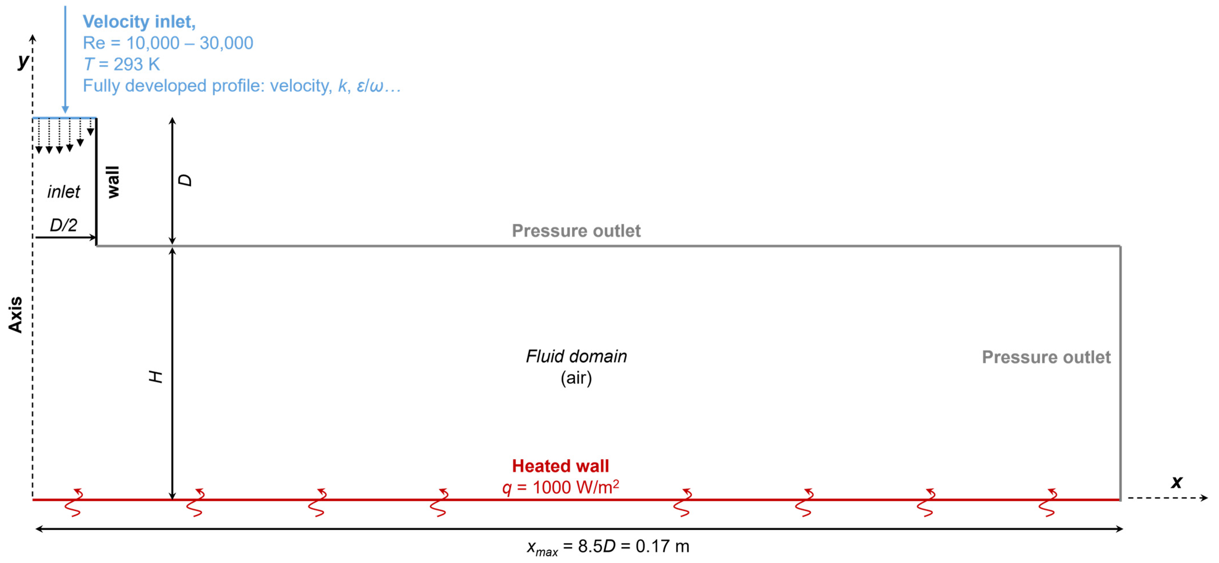
Due to assumptions from Kolmogorov theory implemented in the RANS approach, the 2D axisymmetric models were sufficient to study impinging jet phenomena. It was confirmed by research by Kura et al. [45] and Petera et al. [5], who reported no significant differences in the Nusselt number distribution between 2D and 3D geometries. One of the geometries studied is presented in Figure 1, together with the boundary conditions.

Figure 1. Geometry and boundary conditions. H/D = 2, D = 0.02 m.

For all analyzed cases presented in this article, the inlet part length was equal to one inlet diameter D, and because of the use of a fully developed profile at the inlet, it was unnecessary to extend it. The maximum length (x_max) was set to 8.5D to avoid the influence of the outlet boundary condition on the heat transfer processes occurring near the impingement region. Other researchers [17] claimed that the value of at least 6D is sufficient for this kind of analysis. Preliminary analysis and some studies were performed for geometries with an inlet diameter equal to 0.01 m and others, including the main calculations for a geometry with an inlet diameter equal to 0.02 m. Inlet length, inlet diameter, and domain length were fixed for all four geometrical configurations defined by a dimensionless ratio of domain height H to inlet diameter (H/D = 1, 2, 4, 6). The only dimension changing was the domain height, representing the distance between the inlet and the impinging surface.

The air was used as a working fluid for all considered cases. Due to small temperature differences (<15 K) and based on [30], it was decided to use constant thermophysical properties; the values are presented in Table 3.

Table 3. Thermophysical properties of air defined at a temperature 293 K.

Density ρ, kg/m3	Heat Capacity Cp, J/(kg·K)	Thermal Conductivity λ, W/(m·K)	Dynamic Viscosity μ, Pa·s
1.225	1006.43	0.0242	1.7894·10−5

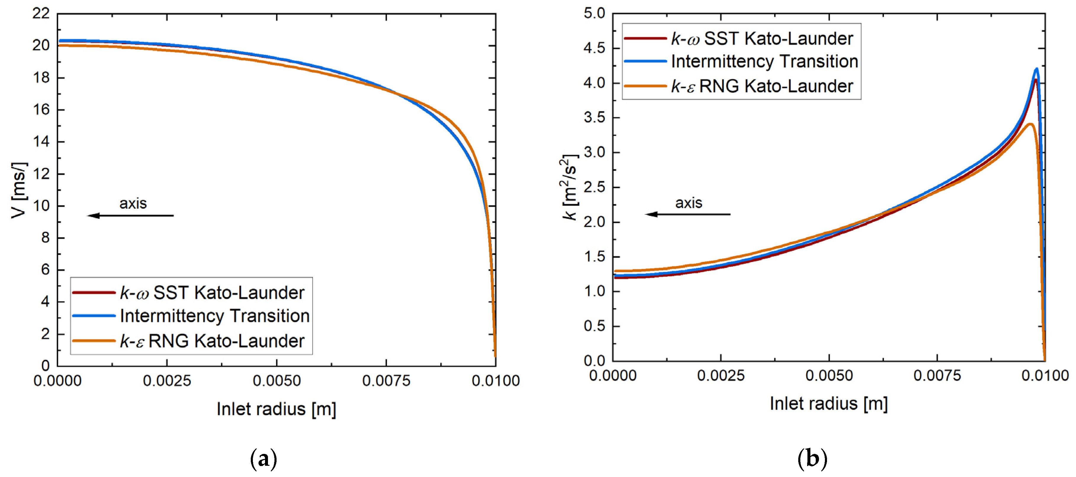
The applied boundary conditions kept for all analyses are presented in Figure 1. Air entered the computational domain with a constant temperature of 293 K. At all Reynolds numbers considered (10,000, 20,000, 23,000, 30,000), a fully developed profile of velocity and other turbulence parameters, i.e., k, ε/ω, etc., was implemented. They were calculated in a separate model (pipe with periodic boundary condition). A comparison between fully developed inlet profiles is presented in Figure 2. The radial velocity component is almost zero (~10⁻¹⁰ m/s), so the magnitude of the velocity was equal to its axial component.

Figure 2. Comparison of fully developed inlet profiles between Intermittency Transition, k-ω SST Kato–Launder, and k-ε RNG Kato–Launder, H/D = 2, D = 0.02 m, Re = 23,000, V_average = 16.8 m/s; (a) velocity magnitude; (b) turbulence kinetic energy.

The comparison between inlet profiles did not show significant differences for k-ω SST Kato–Launder and Intermittency Transition turbulence models. However, the discrepancies between them and k-ε RNG Kato–Launder turbulence models are visible for both velocity and turbulent kinetic energy.

The bottom surface was a wall (no slip) with a constant heat flux of 1000 W/m². All other walls in the model were adiabatic. The pressure outlet (zero gradient) was set for the right and top surfaces.

More in-depth considerations about geometry and boundary conditions are available in the Supplementary File together with an inlet diameter and an inlet profile sensitivity study.

2.2. Discretization

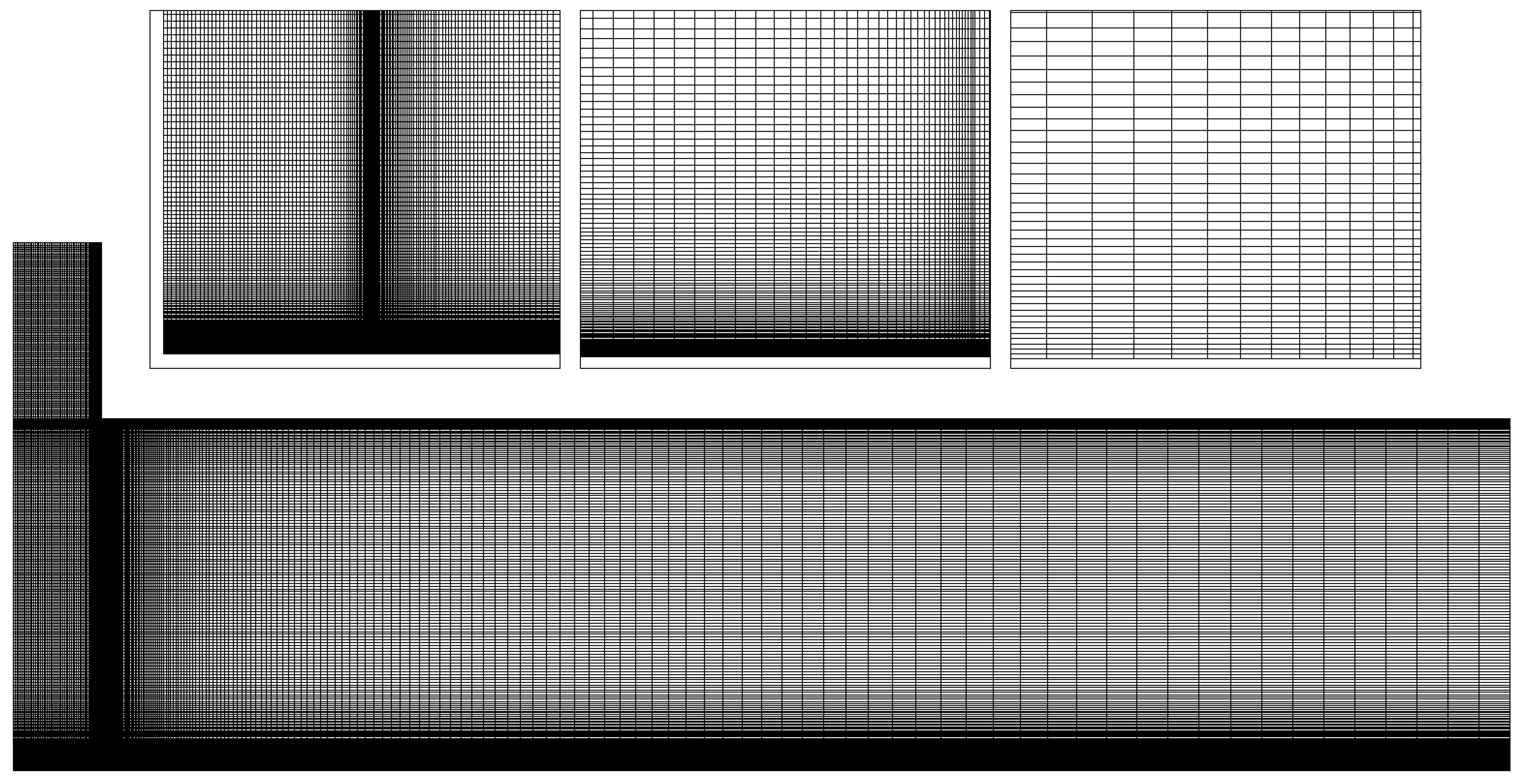
Four block-structured system discretizations of each H/D ratio value (=1, 2, 4, 6) were created. The total element number was between 46,060 and 80,100 at H/D = 1 and H/D = 6, respectively. The inflation layer was applied to all the walls in the model, and the value of y+ was approximately 1 (at the highest Reynolds number value). The exemplary discretization is presented in Figure 3. The local Nusselt number distribution at the heated wall was the most important parameter, so it was selected for the mesh sensitivity study. Figure 4 compares the local Nusselt number distribution at the heated wall for three different meshes and its close-up near stagnation region. The study showed two things: first, the selected mesh (63,100 cells) has passed the grid independence test; second, the local Nusselt number distribution near the stagnation point is sensitive to discretization in that region, which was visible on the coarse grid. Therefore, grid generation in that place must be performed carefully. The mesh sensitivity study was conducted similarly for all other cases and investigations. The grid details are available in the Supplementary File.

Figure 3. Geometry discretization for H/D = 2, D = 0.02 m, y+ < 1, total element number = 63,100.

Figure 4. (a) The local Nusselt number distribution along the heated wall for three selected meshes with y+ up to x/D = 4; (b) close-up of the local Nusselt number distribution up to x/D = 2. k-ω SST Kato–Launder, H/D = 2, D = 0.02 m, Re = 23,000, V_average = 16.8 m/s.

2.3. Numerical Procedure

The numerical calculations were carried out in ANSYS Fluent 18.1. Table 4 presents the general settings of the solver. The SIMPLE algorithm was selected for pressure-velocity coupling, and the gradients were determined using the least squares cell-based method. For spatial discretization of pressure, the second-order scheme was chosen. The second-order upwind scheme was used to calculate the momentum, parameters of turbulence models, and energy equation.

Table 4. Solver general settings.

Solver type: Pressure-based	Flow was incompressible (low value of Mach number, <0.1 at Re = 30,000) [28].
Time: Steady-state	There were no differences between steady-state and transient results, which are discussed in the results section.
Space: 2D axisymmetric	It was explained in the previous section that, due to the Kolmogorov theory’s assumptions regarding turbulence isotropy, there was no difference between 2D and 3D.
Gravity: Disabled	Due to small temperature differences (less than 15 K) and large Reynolds number values (Re > 10,000), it was assumed that buoyancy effects are negligible.

Table 5 presents detailed information on the settings of the turbulence models. In the papers by Seyedein et al. [12], Heyerichs et al. [14], and Zuckerman et al. [43], it was assured that the wall function approach has poor performance in modeling such complex phenomena, and direct solution of the boundary layer heat transfer is required. Therefore, a particular focus was placed on near-wall treatment, and the value of y+ was always kept below 1.

Table 5. Turbulence model options.

Model	Options
k-ω SST	Low-Re correction Production Kato–Launder Production Limiter
k-ε RNG	Enhanced wall treatment Production Kato–Launder Production limiter
Intermittency Transition Model (k-ω SST)	Low-Re correction Production Kato–Launder Production limiter Intermittency Transition Model
Transition SST	Production Kato–Launder Production limiter
$\overline{v^2}\text{-}f$	Default

The selection of a convergence criterion involved stabilizing the average Nusselt number value at the heated surface and ensuring that the residual values equal 10⁻⁶. Additionally, other parameters, such as the outlet’s average velocity, were monitored to assure that the calculations ran smoothly and that the model had no convergence problems. More details on the considerations for convergence and residuals are provided in the Supplementary File.

3. Results

3.1. Preliminary Results

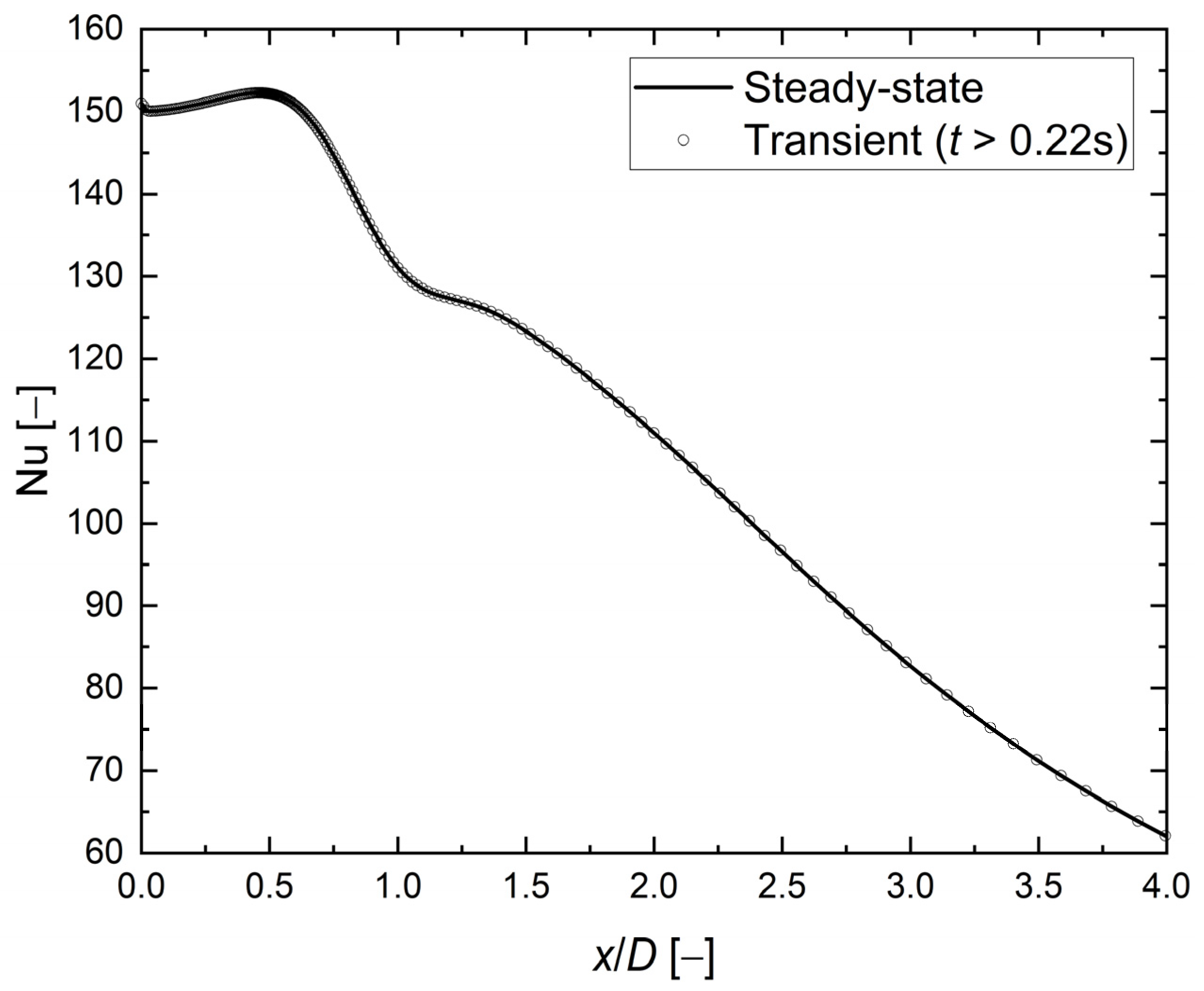
The authors did not find in the literature any explicit justification for why steady-state calculations are suitable for such cases. Therefore, the transient (with timestep equal to 10⁻⁴ s, maximum CFL number equal to 1) and steady-state analysis were performed. It was found that there is no difference between the steady-state and transient models. Figure 5 shows snapshots of the unsteady velocity magnitude at various time steps.

Figure 5. Snapshots of the velocity magnitude, m/s. k-ω SST model, H/D = 2, D = 0.02 m, Re = 23,000.

The propagation of a large vortex structure along the impingement surface is visible. The moment when the structure escapes the computational domain is almost the same time as when the steady state is reached—about 220 ms. Moreover, the same structure is visible during the steady-state calculations, and its development correlates with early oscillations visible on the residuals plot. Figure 6 compares the local Nusselt number values at the heated surface between steady-state and transient calculations. There is a negligible difference; therefore, the steady state approach was selected for further calculations of single turbulent jet impingement.

Figure 6. The local Nusselt number distribution along the heated surface. k-ω SST model, H/D = 2, D = 0.02 m, Re = 23,000.

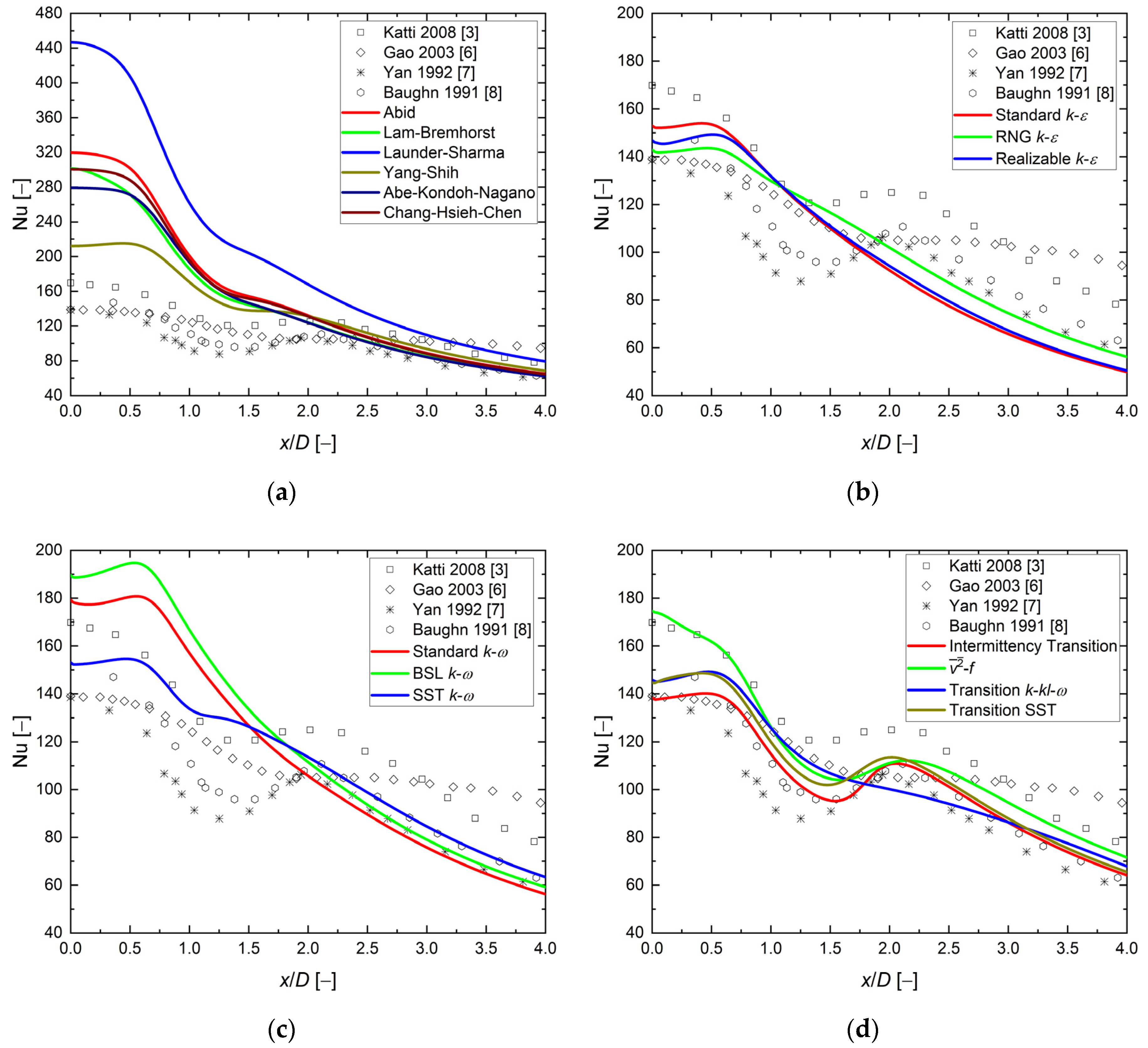
The studies presented in this section represent a necessary step taken before the primary analysis. The purpose was to gain knowledge of the jet impingement phenomenon and its modeling in ANSYS Fluent, select the most suitable turbulence model, and compare the results with other researchers’ numerical and experimental investigations. Figure 7 compares preliminary CFD results and experimental data available in the literature.

Figure 7. Comparison between preliminary numerical results and experimental studies [3,6,7,8]. The local Nusselt number distribution along the heated surface. H/D = 2, D = 0.01 m, Re = 23,000. (a) low-Re k-ε models; (b) k-ε models (enhanced wall treatment, without Kato–Launder limiter); (c) k-ω models (without Kato–Launder limiter); (d) other models.

Based on the first analysis (Figure 7a), the low-Re k-ε models failed to predict local Nusselt number distribution. The incredible overprediction (40–200%) of the Nusselt number in the stagnation zone completely declassifies them for further use. Agreement with the experimental results can be found far from the stagnation point at x/D > 2.5. This investigation confirmed the conclusions of [13,25,46] that the low-Re k-ε models are not suitable for modeling the jet impingement phenomenon. It should be emphasized that this research was conducted to be coherent with all further research.

In the second analysis (Figure 7b), the performance of the k-ε model family was checked. Calculations were performed for three turbulence models with an enhanced wall treatment option and without the Kato–Launder limiter. All three models failed to predict a second Nusselt number maximum. Furthermore, discrepancies were found between the CFD and the experimental results in the stagnation region x/D < 1.5 (overprediction: 2–6%) and far away region x/D > 2.5 (underprediction: 2–12%). The RNG model shows the closest similarity (0.7–2% at x/D < 1.5 and x/D > 2.5, respectively) of the local Nusselt number distribution to that of experimental studies from the k-ε model family. These findings correspond to statements found in the literature [21,25,26,30,32].

The purpose of the third investigation (Figure 7c) was to check the performance of the k-ω model family. Calculations with three turbulence models without the Kato–Launder limiter were performed. Like the k-ε family, all three models failed to predict a second Nusselt number maximum (SST showed an inflection point and small second maxima, but did not match the experimental results), the Nusselt number values in the stagnation region x/D < 1.5 were in even worse correspondence (higher overprediction of the Nusselt number 6–30%). For regions far from the stagnation point x/D > 2.5, the k-ω models performed better than the k-ε model family (2–9%). The SST model exhibited the closest similarity (6–2% at x/D < 1.5 and x/D > 2.5, respectively) of the local Nusselt number distribution to experimental studies. These findings corresponded to statements found in the literature [21,25,26,27,32,43].

The last preliminary analysis (Figure 7d) was designed to check the performance of other turbulence models implemented in ANSYS Fluent. The $\overline{v^2}\text{-}f$ model and three others capable of modeling the laminar-turbulent transition were analyzed. Surprisingly, three models (excepting the k-kl-ω) predicted the second maximum of the Nusselt number and matched the experimental data. Furthermore, the four models were characterized by small discrepancies compared with previous studies in the stagnation region x/D < 1.5 and the farthest away region x/D > 2.5 (1–3% and 1–12%, respectively). The performance of the Intermittency Transition Model appeared to be the best among other models. Furthermore, the $\overline{v^2}\text{-}f$ model agreed well with one experimental data series in the stagnation zone [3]. These findings, like the prediction of the Nusselt number second maximum and the good agreement with experimental data, corresponded to statements found in the literature for the Intermittency Transition Model [5,18,24,25], the Transition SST [19], and the k-kl-ω [24]. The Nusselt number distribution of the $\overline{v^2}\text{-}f$ model was almost constantly offset at approximately 8% higher than the experimental data. However, the findings of other researchers contradicted this statement [13,15,17,28,33,35].

3.1.1. Kato–Launder Limiter

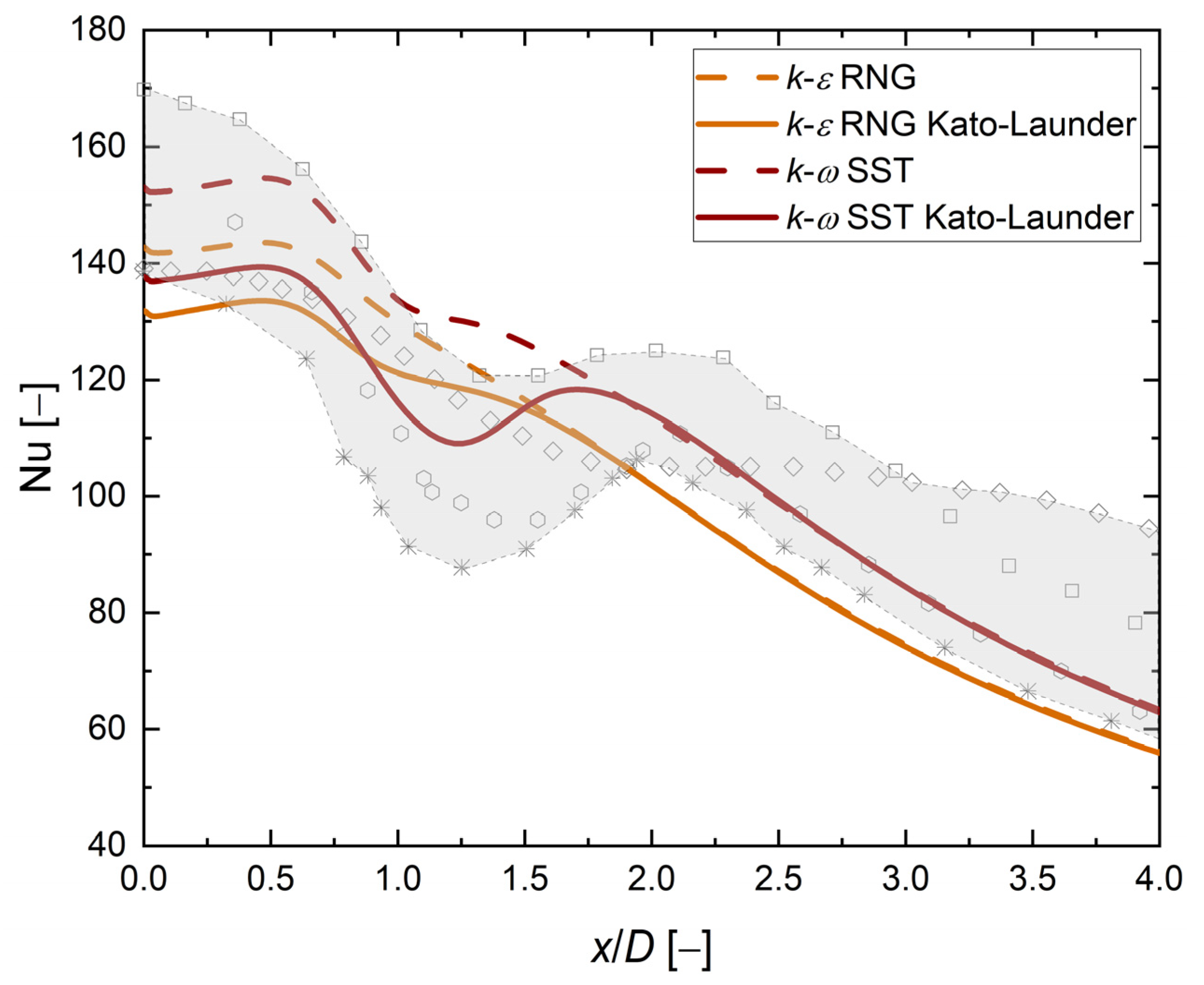
A good performance of the Intermittency Transition Model was brought to the authors’ attention during the preliminary analysis. It was found that this is primarily due to the Kato–Launder (KL) limiter (set on by default). The KL limits the production of turbulent kinetic energy in the stagnation region, which was responsible for overprediction in the Nusselt number distribution [20]. For the last step during the preliminary phase, the influence of KL on the k-ε RNG and k-ω SST models was checked. Figure 8 compares the numerical and experimental results for both models with and without the Kato–Launder limiter.

Figure 8. Influence of the Kato–Launder limiter on the local Nusselt number distribution. k-ε RNG and k-ω SST models, H/D = 2, D = 0.01 m, Re = 23,000. The shaded area represents the experimental results [3,6,7,8].

The influence of the Kato–Launder limiter was visible in the results presented in the stagnation zone x/D < 1.5. The Nusselt number in the region far from the stagnation point x/D > 2 was the same as for the model without the limiter. The Nusselt number value was reduced by 8% and 10% for the k-ε RNG and the k-ω SST models, respectively. Moreover, the local minima and maxima were now clear for the k-ω SST turbulence model and better matched the experimental results in both the values and the shape. These results support the findings of other researchers [5,18,19,20]. Information about the influence of the Kato–Launder limiter on the k-ε RNG turbulence model was not found in the literature. The results show that the limiter applied to the k-ε turbulence model causes a decrease in the Nusselt number in the stagnation region, except at the stagnation point itself, where a decrease of 7% of the underprediction of ~7% of the Nusselt number could be observed. The local Nusselt number distribution calculated using the k-ε RNG Kato–Launder model showed small minima and maxima.

3.1.2. Preliminary Results Summary

The preliminary steps showed that none of the analyzed turbulence models perfectly matched the experimental data. On the other hand, they all laid in the experimental data acceptance limits except for the low-Re, the standard, and the realizable k-ε models. Discrepancies in experimental results were analyzed in [13,42]. The lack of details in experimental procedures and different measurement techniques did not help in the validation of turbulence models of the jet impingement phenomenon [43]. The Intermittency Transition turbulence model seemed to be the best among the other turbulence models. This is why it was selected for the main analysis, together with the $\overline{v^2}\text{-}f$ and the Transition SST turbulence models. The study of the influence of the Kato–Launder limiter on the k-ω SST and the k-ε RNG turbulence models exhibited that both models can be utilized for the primary numerical investigation. Therefore, five turbulence models were selected for further analysis to check their performance for other Reynolds numbers and H/D values.

3.2. RANS vs. DNS

During the analysis, a comparison was made between the RANS calculations and the DNS results available in the literature [41]. Four selected turbulence models were compared with the DNS analysis for the exact geometrical and hydrodynamical conditions: H/D = 2 and Re = 10,000. A fully developed profile (FD) and two profiles from DNS analysis were used: convergent nozzle profile (CNP), which mimics the flat inlet profile, and a long tube profile (LTP) similar to the fully developed one. Figure 9 compares the velocity inlet profiles and the local Nusselt number distribution between the RANS and DNS results.

Figure 9. The local Nusselt number distribution and inlet velocity profile. H/D = 2, D = 0.02 m, Re = 10,000, V_{inlet,average} = 7.30 m/s, V_inlet,max = 8.99 m/s. (a) Nusselt number distribution for DNS and experimental results [4]; (b) comparison of the inlet velocity profile between DNS and RANS Intermittency Transition Model; (c) comparison of the Nusselt number distribution between DNS, RANS (FD), and experimental results [4]; (d) comparison of the Nusselt number distribution between DNS and the RANS Intermittency Transition Model, influence of the inlet profile.

Several observations can be formulated.

First (Figure 9a), only one experimental data set was available for this case and the DNS results did not match it. The authors suggested that this is due to differences in velocity inlet conditions. It is seen that, depending on the type of velocity profile, the DNS results more or less adequately reflected the experimental ones. The convergent nozzle profile seemed to be more suitable for such analysis. However, in the stagnation area, it underpredicted the Nusselt number values, while in the rest of the domain it overpredicted.

Second (Figure 9b), a comparison of the inlet velocities between DNS and the Intermittency Transition Model reveals differences, especially the long tube profile and the fully developed RANS one. Therefore, in our opinion, the long-tube profile is not fully developed.

Third (Figure 9c), none of the RANS models perfectly matched the DNS data in the entire range. The $\overline{v^2}\text{-}f$ results were similar to the LTP DNS between x/D = 0.5 and x/D =1.5. The k-ω SST Kato–Launder and Intermittency Transition models showed fewer discrepancies than the DNS LTP data and match the experimental data almost perfectly far from the stagnation region x/D > 2.5.

Fourth (Figure 9d), the last step in this study was to analyze the Intermittency Transition model with the same velocity inlet profiles as in the DNS study. According to DNS and RANS calculations, the Nusselt number distribution (for x/D < 2) is influenced by the inlet velocity profile. This finding is also corroborated by references [15,16]. The local Nusselt number distribution shape for CNP is similar to the DNS one, with a constant offset of ~5% for small values of x/D < 1. The most significant discrepancies (~22%) and different behavior of the Nusselt number can be found between x/D = 1 and x/D = 2.5. It was mentioned previously that the LTP does not represent a fully developed velocity profile. Minor differences (<2%) in the RANS Nusselt number distribution between LTP and FD profiles support that observation. Moreover, fully developed and flat inlet profiles limit the Nusselt number values, and all not-fully-developed profiles lay between them [15,47]. The enormous overprediction (35%) of the Nusselt number in the stagnation zone in DNS calculations is not supported by any RANS model calculations (except $\overline{v^2}\text{-}f$) and experimental studies.

3.3. Main Results

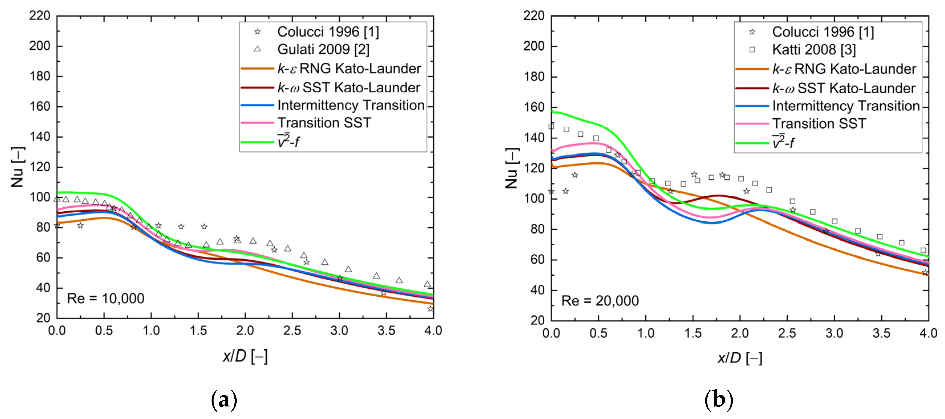
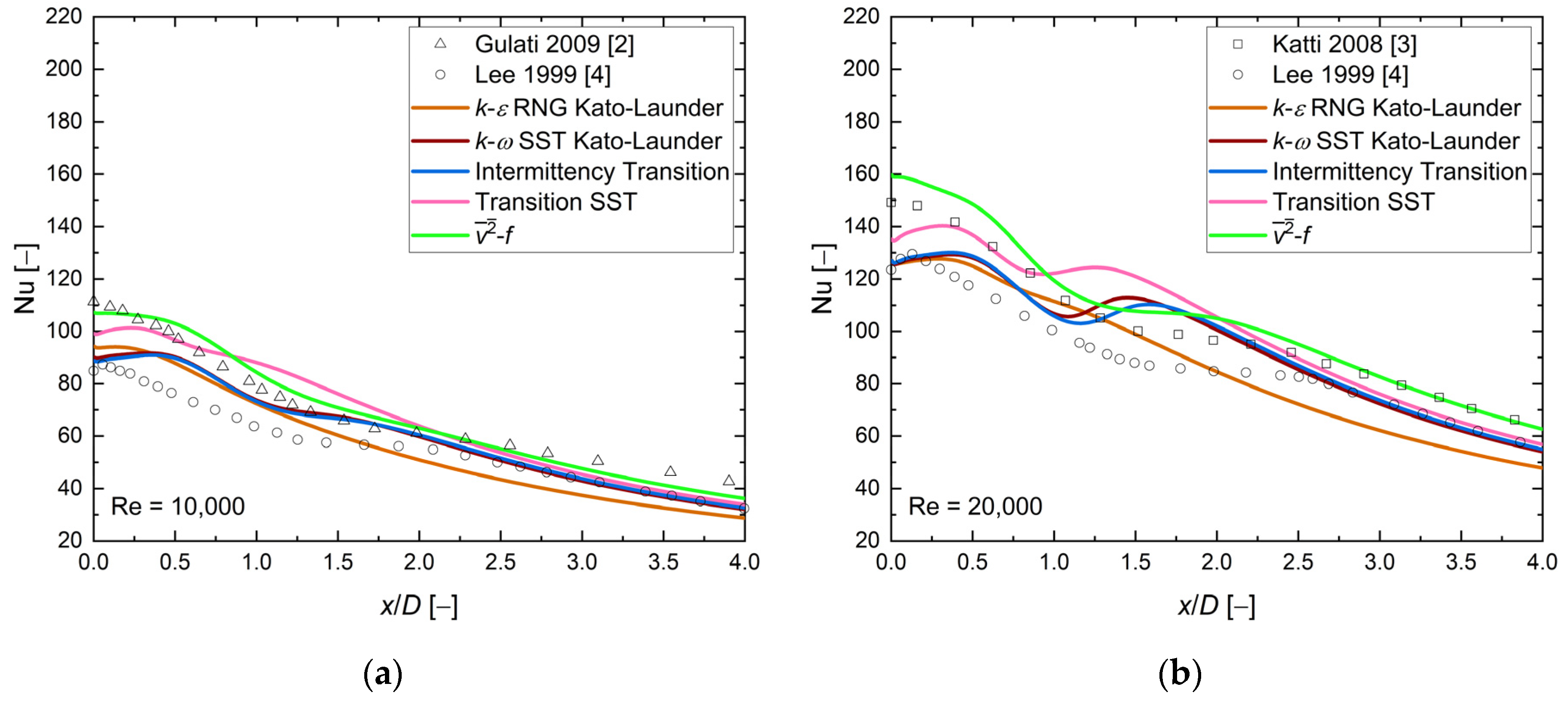
Figure 10 shows local values of the Nusselt number along the heated wall, at H/D = 1 and four values of the Reynolds number.

Figure 10. The local Nusselt number distribution, comparison between CFD RANS results and experimental data [1,2,3]. H/D = 1, D = 0.02, and (a) Re = 10,000, (b) Re = 20,000, (c) Re = 23,000, (d) Re = 30,000.

All experimental data showed a second Nusselt maximum in the region between x/D = 1.5 and x/D = 2.0. Analysis of the CFD results revealed that at Re = 20,000, 23,000, and 30,000, only the k-ω SST Kato–Launder turbulence model indicated local maxima in that region, while local minima of the Nusselt number characterized other models. At Re = 10,000, $\overline{v^2}\text{-}f$, Transition SST and k-ω SST Kato–Launder turbulence models demonstrated weak secondary maxima. Discrepancies in the Nusselt number stagnation point values (20–30%) could be observed for cases where two experimental data sets were available, and all numerical results laid between them, except the $\overline{v^2}\text{-}f$ turbulence model. The k-ε RNG Kato–Launder and $\overline{v^2}\text{-}f$ turbulence models were limiting the values of the Nusselt number, and the results obtained with $\overline{v^2}\text{-}f$ were always higher than k-ε RNG Kato–Launder by ~23–34% and ~20–27% at x/D < 1 and x/D > 2.5, respectively. The shape of the $\overline{v^2}\text{-}f$ model was very close to the experimental data [3] in stagnation region x/D < 1 and the far away region x/D > 2.5 with differences of ~5%. The region where $\overline{v^2}\text{-}f$ failed was the second maxima, at x/D between 1.5 and 2.0.

Based on the available results, the k-ω SST Kato–Launder appeared to be good enough for H/D = 1 and Re = 10,000–30,000 cases.

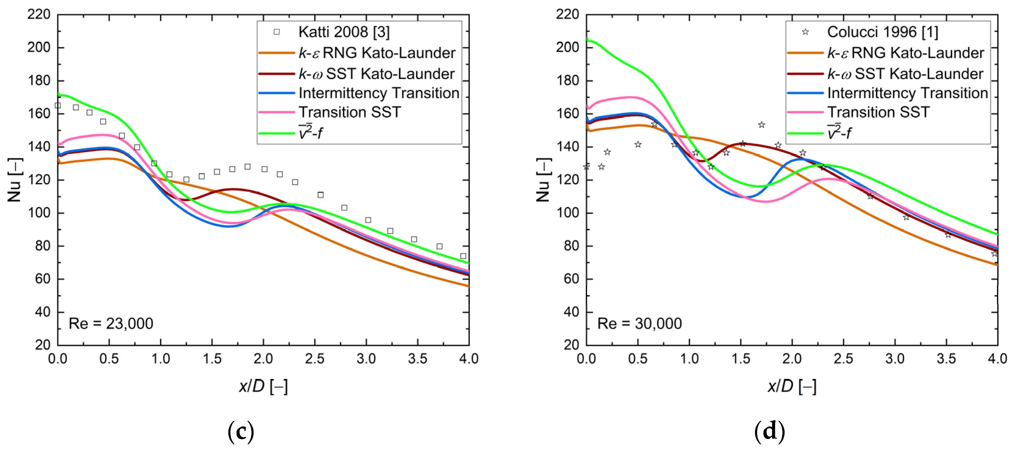
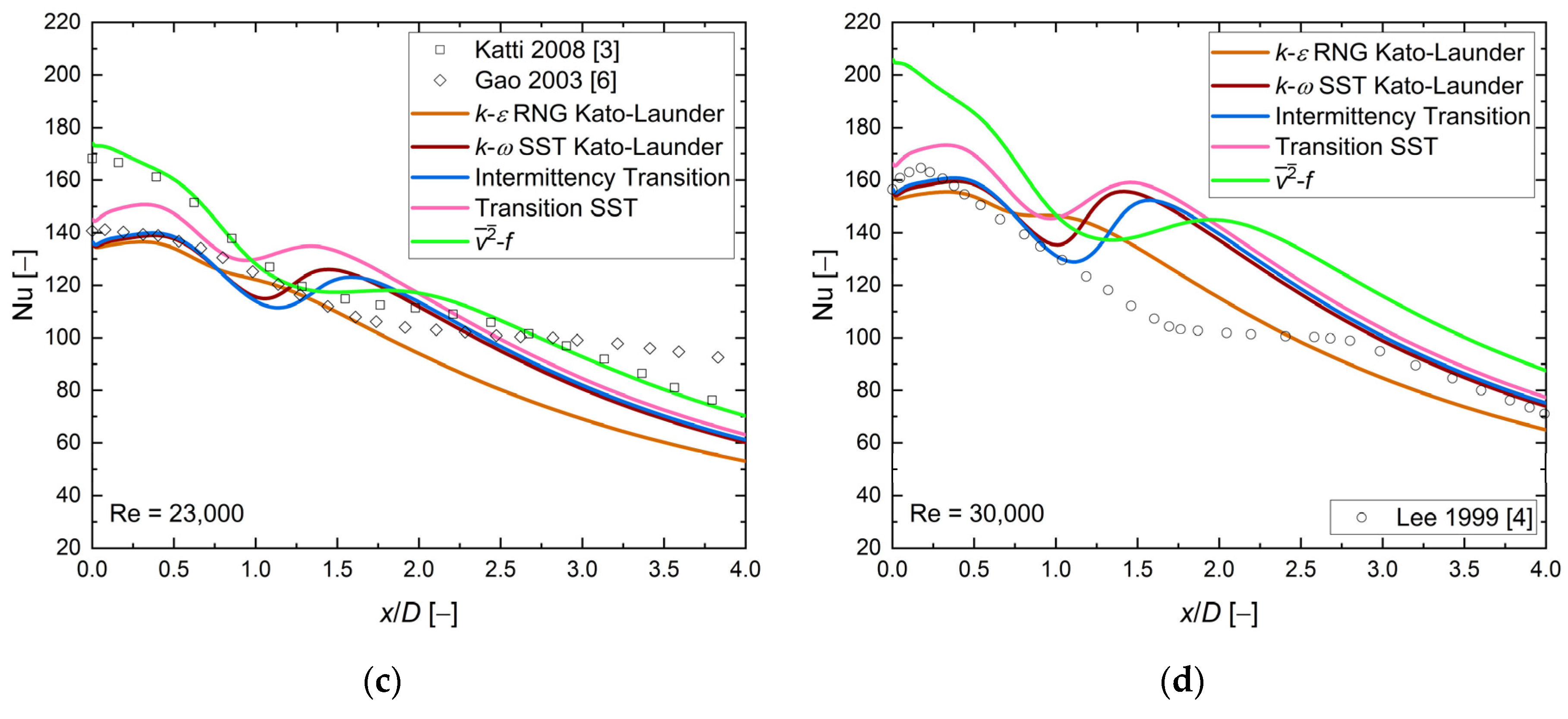
Figure 11 presents the local Nusselt number distribution along the heated wall, at H/D = 2 and four values of the Reynolds number.

Figure 11. The local Nusselt number distribution, comparison between CFD RANS results and experimental data [3,4,5,6,7,8,9]. H/D = 2, D = 0.02, and (a) Re = 10,000, (b) Re = 20,000, (c) Re = 23,000, (d) Re = 30,000.

Like in the case of H/D = 1, all experimental data exhibited a second Nusselt number maxima, but its location seemed to shift toward the outlet, x/D ~1.8 and x/D ~2.0, at H/D = 1 and H/D = 2, respectively. The same movement in the second Nusselt number maximum could be observed for all turbulence models except the k-ω SST Kato–Launder, for which the maxima were visible, whereas other models have had local minima. Moreover, the second maximum was almost in the same place as in the H/D = 1 case. The numerical results looked similar to those of the previous case: the Nusselt number values were limited by the $\overline{v^2}\text{-}f$ and k-ε RNG Kato–Launder turbulence models, the highest values of $\overline{v^2}\text{-}f$ model were in the stagnation point, and there were minor differences between $\overline{v^2}\text{-}f$ and one experimental results series [3] ~1–8%. Analysis of the Re = 23,000 case revealed a large scatter in the experimental data of ~20%, 40%, and 60% at x/D < 1.0, 1.0 < x/D < 2.5, and x/D > 2.5, respectively. All the numerical data, except those from the k-ε RNG Kato–Launder turbulence model, were localized between them. The shape of the local Nusselt number calculated using the Intermittency Transition Model matched the experimental results best in comparison with the others, and the differences between the CFD and experimental data were ~7%, ~5%, and ~4% at x/D < 1.0, 1.0 < x/D < 2.5, and x/D > 2.5, respectively. The comparison of the results with other numerical investigations not presented in Figure 11 is discussed in Table 6.

Table 6. Comparison with other numerical investigations available in the literature. H/D = 2, Re = 20,000, 23,000.

Author	Differences
Re = 20,000
Hadžiabdić et al. [38] (LES) Figure S15a	Similar values and shape of the local Nusselt number distribution in comparison to k-ω SST Kato–Launder, Intermittency Transition and Transition SST turbulence models for x/D < 1.5 were observed; The second Nusselt number maximum in LES was close to Intermittency Transition and $\overline{v^2}\text{-}f$ turbulence models; In a region far from the stagnation point x/D > 2.0, the values of the LES Nusselt number were lower than four RANS models and close to the k-ε RNG Kato–Launder turbulence model.
Re = 23,000
Jensen et al. [17] (RANS) Figure S15b	$\overline{v^2}\text{-}f$ model demonstrated very similar behavior of the local Nusselt number distribution shape compared to the authors’ case, but with an almost constant offset of ~7% below; The source of discrepancies might be a difference in the Reynolds number value, 23,000 (authors) vs. 23,750 (Jensen et al.), but the Nusselt number value increased with increasing Reynolds number values, while in the mentioned paper, an opposite behavior was found for the same turbulence model.
Wienand et al. [20] (RANS) Figure S15c	Comparison of the k-ω SST Kato–Launder turbulence model indicated an overprediction of the Nusselt number at the stagnation point of 3%; The shape of the local Nusselt number distribution at other x/D values was generally the same as that of the authors, but with an almost constant offset of about 17%.
Petera [24] (RANS) Figure S15d	Differences between the Intermittency Transition Model compared with the authors’ calculations of approximately 4–6% for the stagnation region and ~2% at far away regions x/D > 2.0 were found; The local Nusselt number distribution for the Intermittency Transition Model calculated by Petera resembled the authors’ results from the Transition SST turbulence model in the stagnation zone; In the same publication, the k-ω SST turbulence model results could be found, but with a ~18% overprediction of the Nusselt number value at the stagnation point compared with the calculations of the authors. In the region far from the stagnation point, both investigations showed almost the exact behavior of the k-ω SST turbulence model. In this case, the source of the differences was easy to find, and it was the Kato–Launder limiter, which was turned off in Petera’s investigation; In another article by the same researcher [5], he presented the k-ω SST turbulence model with the Kato–Launder limiter, which could be compared with the results of the authors. The differences were smaller by ~4% at the stagnation point, but some discrepancies could still be observed at x/D = 2.0.
Sagot et al. [26] (RANS) Figure S15e	By comparing the results of k-ω SST and k-ε RNG turbulence models, a small difference in the stagnation region (~2% for both models) and a significant one at x/D > 1.0 (~15% for k-ε RNG and 15–30% for k-ω SST) could be observed; Large and almost constant underprediction compared with the authors’ results was found at x/D > 2.5 for both models; The secondary maximum in the local Nusselt number distribution in the k-ω SST turbulence model from Sagot et al. was shifted toward the domain outlet of about one inlet diameter from the authors’ results. The values of the second Nusselt number maximum were also different: 116 (authors) vs. 96 (Sagot et al.); Another interesting observation is that the k-ε RNG turbulence model results of the authors were almost identical to those of the Sagot et al. k-ω SST model at x/D > 2.5.
Ortega-Casanova et al. [27] (RANS) Figure S15f	Comparison of the k-ω SST turbulence model indicated many differences; Overprediction of the Nusselt number value of about 6% at x/D < 0.5 and maximal underprediction of ~16% at higher values of x/D compared with the authors’ case; Local minima and maxima from Ortega-Casanova et al.’s calculations were flatter compared with the authors’ data; Both curves of the Nusselt number local distribution were consistent for x/D > 3.0.
Zhou et al. [28] (RANS) Figure S15g	The shape of the local Nusselt number distribution was similar but lower, with an almost constant offset of ~7% for both $\overline{v^2}\text{-}f$ and k-ε RNG turbulence models compared with the authors’ results; The values of the Nusselt number of the k-ω SST turbulence model were higher ~5% than those of the authors and close to the Transition SST model at x/D < 1.0. At higher values of x/D, the Nusselt number values were lower than the authors’ results of approximately 10%; It is hard to see any local minima and maxima in the local Nusselt number distribution of the k-ω SST turbulence model calculated by Zhou.
Aillaud et al. [36] (LES) Figure S15h	Smaller values of the local Nusselt number compared with the experimental and numerical results of about 15% at x/D < 2.0 and close to k-ε RNG Kato–Launder at higher values of x/D > 2.0 were observed.
Uddin et al. [40] (LES) Figure S15i	LES calculations showed similarities to k-ω SST Kato–Launder and Intermittency Transition turbulence models at the stagnation region x/D < 0.5; At x/D between 2.0 and 3.0, the local Nusselt number distribution from the LES calculations was close to the authors’ k-ε RNG Kato–Launder curve; Between x/D = 0.5 and 2.0 in the Intermittency Transition model, the Nusselt number curve was similar to the LES results, with an average difference of 4%, but both the local minima and maxima were shifted toward the stagnation point of about 0.25D compared with the RANS model; The secondary Nusselt number maximum value was also lower than the Intermittency Transition one of about 3%.

Based on available results, the Intermittency Transition Model appeared to be sufficiently good at H/D = 2 and Re = 10,000–30,000 cases.

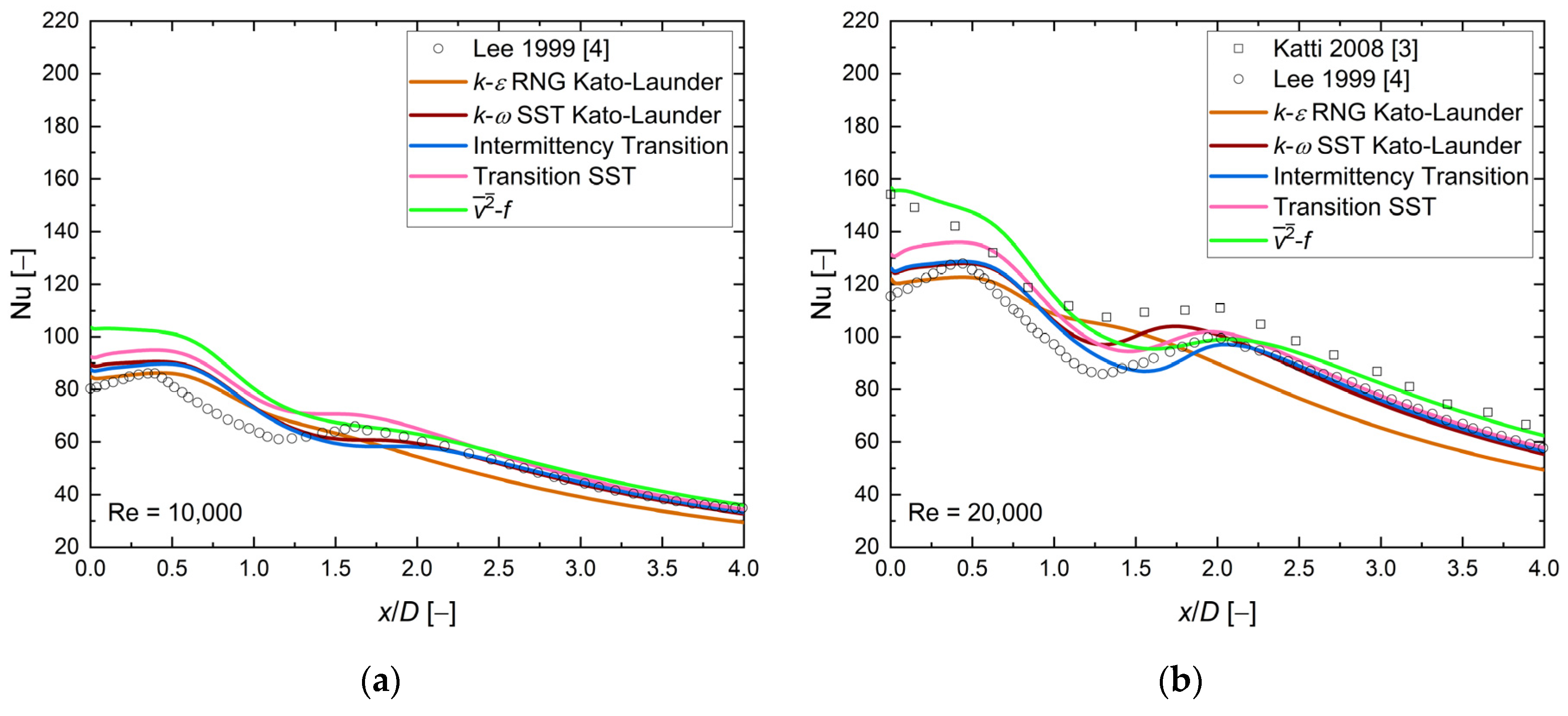
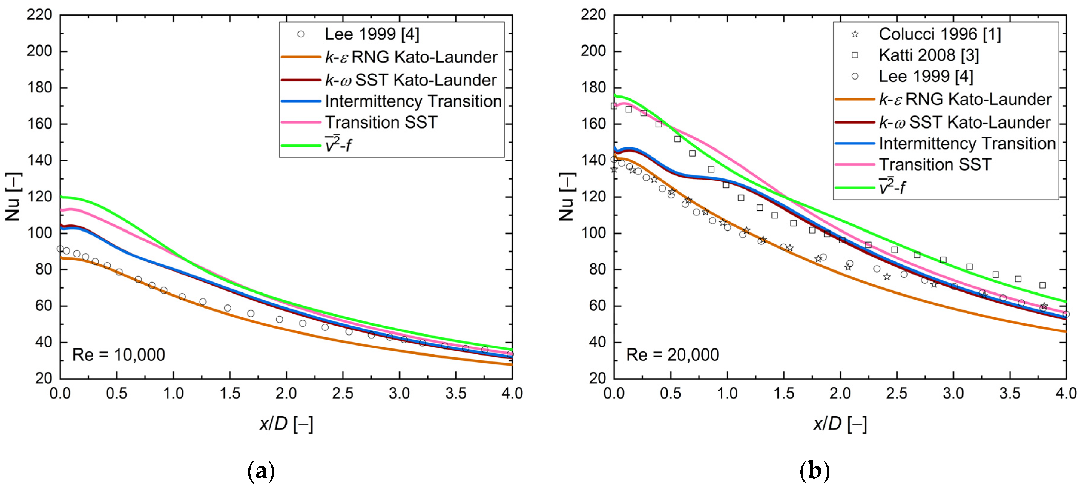
Figure 12 presents the local Nusselt number distribution along the heated wall, at H/D = 4, and four values of the Reynolds number. Analysis of the experimental results barely visualized the maximum of the secondary Nusselt number at Re = 10,000. For higher Reynolds number values, the shape of the second maxima was more evident, especially at Re = 30,000. The results at H/D = 4 continue the trend of shifting the local maxima toward the domain outlet, and for this case, the position of the second Nusselt number maximum was approximately x/D = 2.5. Analysis of the numerical results showed different behavior at Re = 20,000, 23,000, and 30,000, and the secondary Nusselt number maximum location was shifted in the opposite direction, toward the stagnation point, for the k-ω SST Kato–Launder, Transition SST, and Intermittency Transition Model. The $\overline{v^2}\text{-}f$ turbulence model appeared to cause the stable position of the second Nusselt number maximum at x/D = ~2.0. Compared with the previous geometrical configuration, the second Nusselt number maxima were higher by about 8%. Moreover, an application of turbulence models like k-ω SST Kato–Launder, Transition SST, and Intermittency Transition entailed the local maximum in a region where the $\overline{v^2}\text{-}f$ turbulence model posessed its local minimum. The numerical results have shown a similar behavior to the two previous cases: the Nusselt number values were limited by $\overline{v^2}\text{-}f$ and k-ε RNG Kato–Launder turbulence models, the highest values of the $\overline{v^2}\text{-}f$ model were in the stagnation point, and there were minor differences between $\overline{v^2}\text{-}f$ and one experimental results series [3] ~1–13%. The analysis of the numerical results focused only on the local Nusselt number distribution shape exhibited that all the presented turbulence models failed. On the other hand, an analysis based on the Nusselt number values revealed that at x/D < 1.0 and Re = 20,000, 23,000, and 30,000, all turbulence models caused values close to or between the experimental data, with small discrepancies of about 3–9%.

Figure 12. The Local Nusselt number distribution, comparison between CFD RANS results and experimental data [2,3,4,6]. H/D = 4, D = 0.02, and (a) Re = 10,000, (b) Re = 20,000, (c) Re = 23,000, (d) Re = 30,000.

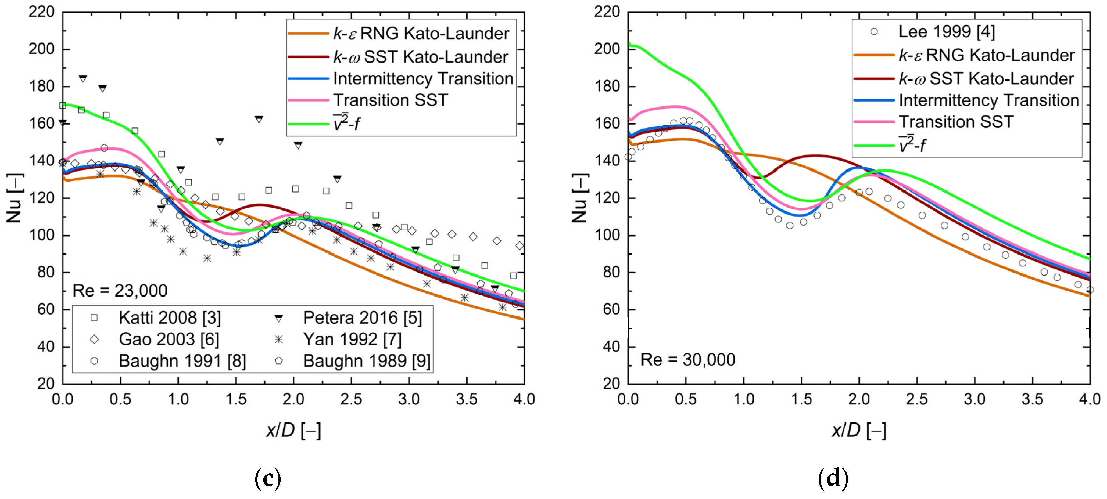
Heat transfer analysis at all presented Reynolds numbers at the stagnation point showed small differences between the numerical and experimental data for the three turbulence models k-ε RNG Kato–Launder, k-ω SST Kato–Launder, and Intermittency Transition of about 1–9%. Analysis of the heat transfer for regions far from the stagnation point x/D > 2 indicated, at Re = 10000, that all turbulence models were between experimental data sets except the k-ε RNG Kato–Launder model, whose results differed by about 15%. Three turbulence models (k-ω SST Kato–Launder, Intermittency Transition, and Transition SST) were close to the experimental data at the region far from the stagnation point at Re = 10,000, 20,000, and 30,000. The $\overline{v^2}\text{-}f$ turbulence model was the closest to the experimental results at the Re = 23,000 case. An analysis of the shape of the local Nusselt number distribution showed that the k-ε RNG Kato–Launder model was characterized by the smallest local minima and maxima compared with other models.

Based on the available results, the k-ε RNG Kato–Launder model appeared to be sufficiently good at H/D = 4 and Re = 10,000–30,000 cases.

Figure 13 presents the local Nusselt number distribution along the heated wall for the last geometrical configuration H/D = 6 and four values of the Reynolds number.

Figure 13. The local Nusselt number distribution, comparison between CFD RANS results and experimental data [1,3,4,6,7,8,9,10,11]. H/D = 6, D = 0.02, and (a) Re = 10,000, (b) Re = 20,000, (c) Re = 23,000, (d) Re = 30,000.

The experimental results analysis showed no visible local maxima of the Nusselt number values in the entire range and all four Reynolds number values. The experimental results at Re = 23,000 indicated a large scatter in the entire range of x/D, about 26%. The numerical results presented a clear secondary Nusselt number maximum for k-ω SST Kato–Launder, Intermittency Transition, and Transition SST turbulence models at Re = 20,000, 23,000, and 30,000. The $\overline{v^2}\text{-}f$ model was an exception: a local Nusselt maximum was visible at Re = 30,000. The only turbulence model consistent with the experimental data based on the local Nusselt number distribution shape was the k-ε RNG Kato–Launder turbulence model. At all four Reynolds number values, the k-ε RNG Kato–Launder turbulence model was close to the experimental data at x/D < 2.5, the discrepancies were visible at higher values of x/D, and average differences in the Nusselt number values were about 18%. Analysis of the numerical results based on the Nusselt number values exhibited that for two cases (Re = 20,000 and 23,000) where more than one experimental data set was available, all turbulence modes fit the experimental data. Local Nusselt number distribution for both the $\overline{v^2}\text{-}f$ and Transition SST turbulence models were close to each other at x/D < 1.5. The numerical results showed a similar behavior to the previous cases: the Nusselt number values were limited by the $\overline{v^2}\text{-}f$ and k-ε RNG Kato–Launder turbulence models, the highest values of the $\overline{v^2}\text{-}f$ model were in the stagnation point, and there were small differences between $\overline{v^2}\text{-}f$ and one experimental results series [3] ~2–13%. Another observation was (like in the previous case) a shift of the second Nusselt number maximum location for CFD results towards the stagnation point to x/D = ~1.0, for k-ω SST Kato–Launder, Intermittency Transition, and Transition SST turbulence models. Table 7 compares the authors’ results with other numerical investigations.

Table 7. Comparison with other numerical investigations available in the literature. H/D = 6, Re = 23,000.

Author	Differences
Behnia et al. [15] (RANS) Figure S15j	Comparison of $\overline{v^2}\text{-}f$ turbulence models showed similarities in the stagnation region x/D < 1.0 with differences of 2–7%; At higher values of x/D (>2) the $\overline{v^2}\text{-}f$ results by Behnia et al. were close to the authors’ k-ε RNG Kato–Launder turbulence model values with a difference of about 8%.
Petera [24] (RANS) Figure S15k	Comparison of the Intermittency Transitions turbulence models indicated various behavior in the stagnation region x/D < 1.5 with ~4–18% differences. For regions far from the stagnation point, the differences were smaller (~3–4%) and close to each other; The local Nusselt number distribution from the Intermittency Transition turbulence model by Petera was almost the same as the results of the Transition SST turbulence model of the authors, with an average difference of about 1%; Comparison of the k-ω SST models showed similarities at x/D > 1.0 with differences less than 1% and differences in the stagnation region equal to ~5%. The source of the utilization of the differences was the Kato–Launder limiter.
Wienand et al. [20] (RANS) Figure S15l	Comparison of the k-ω SST Kato–Launder turbulence model indicated completely different behavior at the stagnation point and at x/D > 1 with differences of ~12%; At the x/D > 2.5, results from k-ω SST Kato–Launder by Wienand et al. were close to the authors’ k-ε RNG Kato–Launder turbulence model with an average difference of less than 1%.

Based on available results, the k-ε RNG Kato–Launder model appeared to be sufficiently good at H/D = 6 and Re = 10,000–30,000 cases.

4. Measure of the Differences

The scatter in the experimental data was already known in the community [5,13,15,42,43]. This article confirmed that numerical investigations have similar problems [16]. As was shown before, there are many differences between the numerical results. In some cases, the source of the differences was easy to identify, like different inlet profiles, the Kato–Launder limiter, and the type of boundary condition at the heated surface (constant temperature vs. constant heat flux). For other cases, it was difficult to find one primary source of the differences, and it might have been the various inlet diameter, mesh, solver, turbulence models implementation, etc. Usually, there was more than one source, and without all the information about numerical setup, etc., it is almost impossible to compare CFD results.

Analysis of all presented numerical results allowed the authors to make a few interesting observations. The results of the $\overline{v^2}\text{-}f$ turbulence model were characterized by the global maximum in the stagnation point for all analyzed geometrical configurations and Reynolds numbers, and it was always higher than for other turbulence models. The stagnation point heat transfer analysis indicated that the results of other models have had their local maxima at H/D = 1, 2, and 4. The global maxima at the stagnation point could be seen at H/D = 6 for all turbulence models. The first Nusselt number maximum, a global one at H/D = 1, 2, and 4, was placed at about x/D = ~0.5 at H/D = 1 and 2, and H/D = 4 was moving toward the stagnation point. The last geometric configuration (H/D = 6) caused a change in the behavior of the local Nusselt distribution curve, the first Nusselt number maximum became a local one, and its location was even more shifted (compared with the previous case) in the direction of the axis. The numerical results showed that, with an increasing value of H/D, the position of the secondary Nusselt number maximum moved toward the stagnation point, which was an opposite observation compared with the experimental results. Analysis of the local Nusselt number distribution calculated using the k-ω SST Kato–Launder, Intermittency Transition, and Transition SST turbulence models demonstrated that at H/D = 1 and 2, the first one exhibits a higher magnitude of the second Nusselt number maximum. It was closer to the stagnation point than for the other two models. At higher values of H/D, the Transition SST turbulence model gave a higher value of the second Nusselt number maximum, and its position was close to the axis. Both turbulence models, k-ω SST Kato–Launder and Intermittency Transition, caused a similar tendency at H/D = 4 and almost the same at H/D = 6. The Intermittency Transition Model is based on k-ω SST with a modification, and is capable of representing the laminar to turbulent transition, with almost the same local Nusselt number distribution at H/D = 6 suggesting that the influence of the modification decreased with an increasing H/D ratio. At H/D = 4 (k-ω SST Kato–Launder, Intermittency Transition, and Transition SST) and H/D = 6 (k-ω SST Kato–Launder and Intermittency Transition), the results possessed ‘artificial’ secondary maxima in the local Nusselt number distribution, which were not confirmed by the experimental data. All three models had in common the Kato–Launder limiter and the last two the laminar to turbulent transition, so one of those two options was responsible for this ‘artificial’ secondary maxima, and this problem requires further investigation. Based on the figures presented, the geometrical configuration H/D ratio significantly influenced the behavior of the local Nusselt number distribution/turbulence models more than the Reynolds number. At a constant value of H/D, the change in Reynolds number values made the differences between models easier to see.

Another interesting question was why the local Nusselt number distribution calculated by the authors with one turbulence model looked very similar to the different turbulence model results calculated by others. Numerical analysis of turbulent flow usually requires selecting the proper turbulence model, but the lack of standardized validation makes selecting the turbulence model difficult. Another aspect that is even more important and makes reproducibility of the numerical results almost impossible is the lack of a proper numerical results database with all the critical information. That is why the authors tried to present 80 different numerical results conducted in the same setup with the same solver, etc. Additionally, each important piece of information (Nusselt number distribution values, inlet profiles, meshes) not included in the text is available in the Supplementary File and the repository, together with the Fluent case and data files for each of the 80 calculated cases [48].

Proposal of the Measure

Discrepancies in the local Nusselt distribution between numerical and experimental investigations have been presented. Sometimes, local heat transfer analysis was less important than the overall heat transfer performance of selected turbulence models and its comparison with the experimental data. Therefore, a quantitative measure of discrepancies was proposed. The area under the local Nusselt number distribution curve was selected as a parameter for such analyses. Because the Nusselt number can be considered to be the ratio of the heat rate transferred by convection to the heat rate transferred by conduction, the area can represent the overall value of this ratio. The area for each turbulence model, Reynolds number, and H/D ratio was calculated, and then an averaging operation was performed. The last step was the calculation of the absolute and relative differences between the numerical and experimental data. The equations are presented below:

$$∆{Nu}_{area}=\left|{Nu}_{area,experiment}^{average}-{Nu}_{area,CFD}\right|$$

(7)

$$∆\mathrm{\%}{Nu}_{area}=\frac{\left|{Nu}_{area,experiment}^{average}-{Nu}_{area,CFD}\right|}{{Nu}_{area,experiment}^{average}}$$

(8)

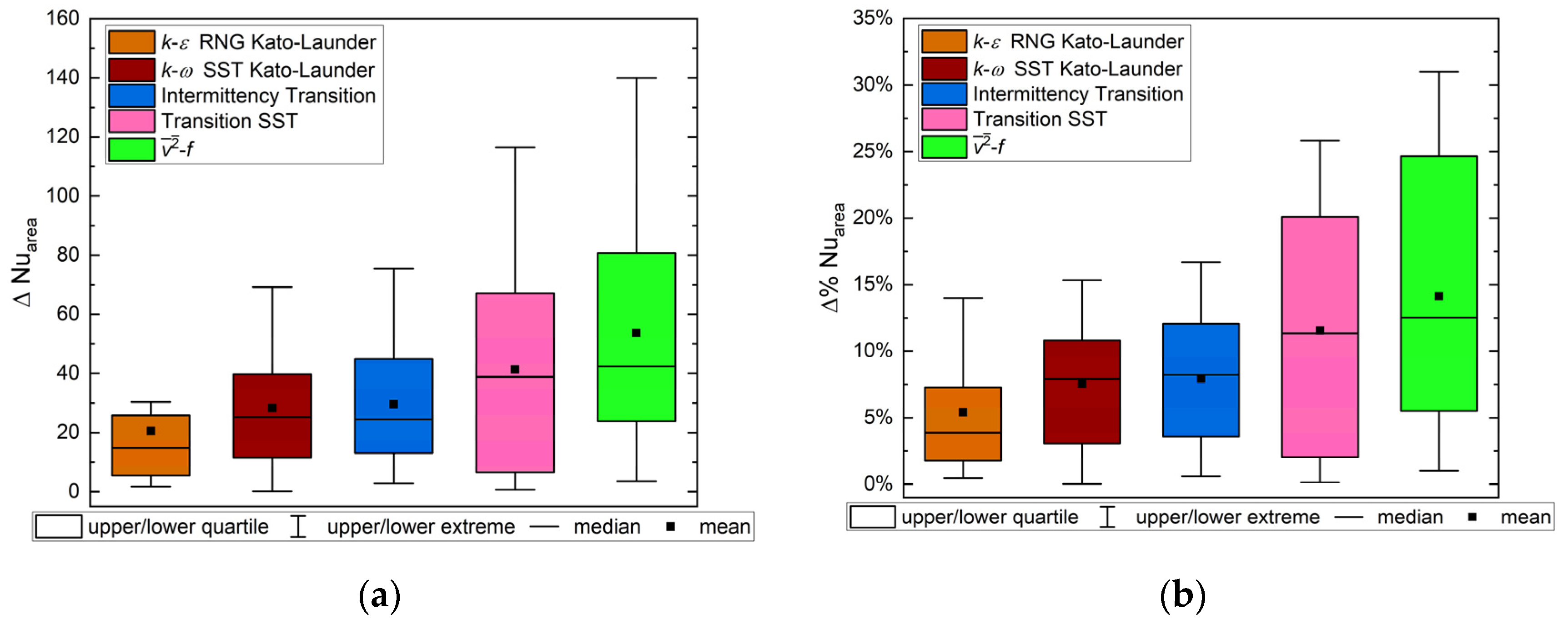
The output of this study was a matrix—for each Reynolds number and H/D ratio, the relative and absolute differences for each turbulent model were obtained. To streamline the analysis, statistical data for each turbulence model were computed across the entire spectrum of the Reynolds numbers and H/D ratios. Figure 14 presents the box and whisker plot, which summarizes this investigation.

Figure 14. Comparison of the area under the local Nusselt number curve between RANS and the experimental results. H/D = 1, 2, 4, 6; Re = 10,000, 20,000, 23,000, 30,000. (a) Absolute difference; (b) relative difference.

Both plots indicated upper and lower extremes and quartile and median differences between RANS and experimental average surface values under the local Nusselt number distribution. Analysis of the plots revealed that the k-ε RNG Kato–Launder turbulence model demonstrated the smallest discrepancies in the entire range of calculations. The Transition SST and $\overline{v^2}\text{-}f$ turbulence models are characterized by the most significant differences in the entire range, both in maximal values and medians. The clear difference between the first three and the last two models was visible. The results of this study also confirmed similarities between the k-ω SST Kato–Launder and Intermittency Transition turbulence models. The first three models had median differences below 10% and maximal values of about 15%. Therefore, considering the quantitative and qualitative points of view together with a local and overall analysis of heat transfer and the computational cost of RANS models of the jet impingement phenomenon for all selected turbulence models with the entire range of H/D and Reynolds number values, the final selection of the proper turbulence models could be completed. Both the k-ω SST Kato–Launder and Intermittency Transition turbulence models appeared to be sufficiently good at H/D = 1, 2, and 4 (with caution). At higher values of the H/D ratio, the k-ε RNG Kato–Launder turbulence model appeared to be a better choice.

5. Discussion and Summary

This paper presents the numerical setup of five turbulence models, four geometrical configurations, and four Reynolds number values. A total of 80 cases were presented, which could serve as a database of RANS calculations of round, turbulent jet phenomena. The authors have also presented a preliminary analysis of their investigation, including some selected studies, such as the influence of the Kato–Launder limiter on both the k-ω SST and k-ε RNG turbulence models and a comparison between steady-state and transient calculations. Furthermore, this paper presented a comparison analysis with experimental data, DNS, RANS, and LES. The study of local heat transfer has been enriched by an overall heat transfer comparison. After considering all the viewpoints mentioned, it is possible to arrive at some general conclusions:

• Scatter in numerical results exists, and lack of detailed information about setup makes comparisons difficult;
• The Kato–Launder limiter reduced the overprediction of the values of the Nusselt number in the stagnation region in the k-ω SST and k-ε RNG turbulence models;
• The second Nusselt number maximum location depended strongly on the H/D values;
• The second Nusselt number maximum was shifted toward the stagnation point with increasing values of H/D;
• The geometry configuration H/D had a bigger influence on the local Nusselt number distribution shape than the Reynolds number;
• Analysis of the the total heat transfer of turbulence models indicated that the k-ε RNG Kato–Launder model was characterized by smaller differences for all the cases—a median difference between the calculated and experimental results was less than 5%. Two additional models with a median difference below 10% are k-ω SST Kato–Launder and Intermittency Transition turbulence models;
• k-ω SST Kato–Launder and Intermittency Transition turbulence models are recommended at H/D = 1 and 2 (Re = 10,000, 20,000, 23,000, and 30,000);
• k-ε RNG Kato–Launder turbulence model is recommended at H/D = 4 and 6 (Re = 10,000, 20,000, 23,000, 30,000).

References

- Colucci, D.W.; Viskanta, R. Effect of nozzle geometry on local convective heat transfer to a confined impinging air jet. Exp. Therm. Fluid Sci. 1996, 13, 71–80. [Google Scholar] [CrossRef]
- Gulati, P.; Katti, V.; Prabhu, S.V. Influence of the shape of the nozzle on local heat transfer distribution between smooth flat surface and impinging air jet. Int. J. Therm. Sci. 2009, 48, 602–617. [Google Scholar] [CrossRef]
- Katti, V.; Prabhu, S.V. Experimental study and theoretical analysis of local heat transfer distribution between smooth flat surface and impinging air jet from a circular straight pipe nozzle. Int. J. Heat Mass Transf. 2008, 51, 4480–4495. [Google Scholar] [CrossRef]
- Lee, J.; Lee, S.-J. Stagnation Region Heat Transfer of a Turbulent Axisymmetric Jet Impingement. Exp. Heat Transf. 1999, 12, 137–156. [Google Scholar] [CrossRef]
- Petera, K.; Dostál, M. Heat transfer measurements and CFD simulations of an impinging jet. EPJ Web Conf. 2016, 114, 02091. [Google Scholar] [CrossRef]
- Gao, N.; Sun, H.; Ewing, D. Heat transfer to impinging round jets with triangular tabs. Int. J. Heat Mass Transf. 2003, 46, 2557–2569. [Google Scholar] [CrossRef]
- Yan, X.; Baughn, J.W.; Mesbah, M. The effect of Reynolds number on the heat transfer distribution from a flat plate to an impinging jet. In Proceedings of the ASME Winter Annual Meeting, Anaheim, CA, USA, 8–13 November 1992; Volume 226, pp. 1–7. [Google Scholar]
- Baughn, J.W.; Hechanova, A.E.; Yan, X. An Experimental Study of Entrainment Effects on the Heat Transfer from a Flat Surface to a Heated Circular Impinging Jet. J. Heat Transf. 1991, 113, 1023–1025. [Google Scholar] [CrossRef]
- Baughn, J.W.; Shimizu, S. Heat Transfer Measurements from a Surface with Uniform Heat Flux and an Impinging Jet. J. Heat Transf. 1989, 111, 1096–1098. [Google Scholar] [CrossRef]
- Lytle, D.; Webb, B.W. Air jet impingement heat transfer at low nozzle-plate spacings. Int. J. Heat Mass Transf. 1994, 37, 1687–1697. [Google Scholar] [CrossRef]
- Lee, D.H.; Song, J.; Jo, M.C. The Effects of Nozzle Diameter on Impinging Jet Heat Transfer and Fluid Flow. J. Heat Transf. 2004, 126, 554–557. [Google Scholar] [CrossRef]
- Seyedein, S.H.; Hasan, M.; Mujumdar, A.S. Modelling of a single confined turbulent slot jet impingement using various k–ϵ turbulence models. Appl. Math. Model. 1994, 18, 526–537. [Google Scholar] [CrossRef]
- Behnia, M.; Ooi, A.; Gregory, P. Prediction of turbulent heat transfer in impinging jet geometries. WIT Trans. State Art Sci. Eng. 2005, 15, 135–163. [Google Scholar] [CrossRef]
- Heyerichs, K.; Pollard, A. Heat transfer in separated and impinging turbulent flows. Int. J. Heat Mass Transf. 1996, 39, 2385–2400. [Google Scholar] [CrossRef]
- Behnia, M.; Parneix, S.; Shabany, Y.; Durbin, P.A. Numerical study of turbulent heat transfer in confined and unconfined impinging jets. Int. J. Heat Fluid Flow 1999, 20, 1–9. [Google Scholar] [CrossRef]
- Kura, T.; Wajs, J.; Fornalik-Wajs, E.; Kenjeres, S.; Gurgul, S. Thermal and Hydrodynamic Phenomena in the Stagnation Zone—Impact of the Inlet Turbulence Characteristics on the Numerical Analyses. Energies 2021, 14, 105. [Google Scholar] [CrossRef]
- Jensen, M.V.; Walther, J.H. Numerical Analysis of Jet Impingement Heat Transfer at High Jet Reynolds Number and Large Temperature Difference. Heat Transf. Eng. 2013, 34, 801–809. [Google Scholar] [CrossRef]
- Huang, H.; Sun, T.; Zhang, G.; Sun, L.; Zong, Z. Modeling and computation of turbulent slot jet impingement heat transfer using RANS method with special emphasis on the developed SST turbulence model. Int. J. Heat Mass Transf. 2018, 126, 589–602. [Google Scholar] [CrossRef]
- Granados-Ortiz, F.J.; Ortega-Casanova, J.; Lai, C.-H. Uncertainty quantification and modelling of CFD simulations of a swirling turbulent jet created by a rotating pipe for application to heat transfer from a heated solid flat plate. In Proceedings of the 1st International Conference on Uncertainty Quantification in Computational Sciences and Engineering (UNCECOMP 2015), Crete Island, Greece, 25–27 May 2015. [Google Scholar] [CrossRef][Green Version]
- Wienand, J.; Riedelsheimer, A.; Weigand, B. Numerical study of a turbulent impinging jet for different jet-to-plate distances using two-equation turbulence models. Eur. J. Mech. B/Fluids 2017, 61, 210–217. [Google Scholar] [CrossRef]
- Simionescu, Ş.-M.; Bălan, C. CFD Study on Convective Heat Exchange between Impinging Gas Jets and Solid Surfaces. Energy Procedia 2016, 85, 481–488. [Google Scholar] [CrossRef][Green Version]
- Caggese, O.; Gnaegi, G.; Hannema, G.; Terzis, A.; Ott, P. Experimental and numerical investigation of a fully confined impingement round jet. Int. J. Heat Mass Transf. 2013, 65, 873–882. [Google Scholar] [CrossRef]
- Chen, K.; Jiang, P.-X.; Chen, J.-N.; Xu, R.-N. Numerical Investigation of Jet Impingement Cooling of a Flat Plate with Carbon Dioxide at Supercritical Pressures. Heat Transf. Eng. 2018, 39, 85–97. [Google Scholar] [CrossRef]
- Petera, K. Turbulent heat transport and its anisotropy in an impinging jet. EPJ Web Conf. 2015, 92, 02063. [Google Scholar] [CrossRef]
- Hofmann, H.M.; Kaiser, R.; Kind, M.; Martin, H. Calculations of Steady and Pulsating Impinging Jets—An Assessment of 13 Widely used Turbulence Models. Numer. Heat Transf. Part B Fundam. 2007, 51, 565–583. [Google Scholar] [CrossRef]
- Sagot, B.; Antonini, G.; Christgen, A.; Buron, F. Jet impingement heat transfer on a flat plate at a constant wall temperature. Int. J. Therm. Sci. 2008, 47, 1610–1619. [Google Scholar] [CrossRef]
- Ortega-Casanova, J.; Granados-Ortiz, F.J. Numerical simulation of the heat transfer from a heated plate with surface variations to an impinging jet. Int. J. Heat Mass Transf. 2014, 76, 128–143. [Google Scholar] [CrossRef]
- Zhou, T.; Xu, D.; Chen, J.; Cao, C.; Ye, T. Numerical analysis of turbulent round jet impingement heat transfer at high temperature difference. Appl. Therm. Eng. 2016, 100, 55–61. [Google Scholar] [CrossRef]
- Buchlin, J.M. Convective Heat Transfer in Impinging-Gas-Jet Arrangements. J. Appl. Fluid Mech. 2011, 4, 137–149. [Google Scholar] [CrossRef]
- Isman, M.K.; Pulat, E.; Etemoglu, A.B.; Can, M. Numerical Investigation of Turbulent Impinging Jet Cooling of a Constant Heat Flux Surface. Numer. Heat Transf. Part A Appl. 2008, 53, 1109–1132. [Google Scholar] [CrossRef]
- Nabadavis, A.; Mishra, D.P. Numerical investigation of jet impingement heat transfer on a flat plate. Carbon Sci. Technol. 2016, 8, 1–12. [Google Scholar]
- Sharif, M.A.R.; Mothe, K.K. Evaluation of Turbulence Models in the Prediction of Heat Transfer Due to Slot Jet Impingement on Plane and Concave Surfaces. Numer. Heat Transf. Part B Fundam. 2009, 55, 273–294. [Google Scholar] [CrossRef]
- Kura, T.; Fornalik-Wajs, E.; Wajs, J.; Kenjeres, S. Turbulence models impact on the flow and thermal analyses of jet impingement. MATEC Web Conf. 2018, 240, 01016. [Google Scholar] [CrossRef]
- Kura, T.; Fornalik-Wajs, E.; Wajs, J.; Kenjeres, S. Heat transfer intensification by jet impingement—Numerical analysis using RANS approach. E3S Web Conf. 2019, 108, 01025. [Google Scholar] [CrossRef]
- Kura, T.; Fornalik-Wajs, E.; Wajs, J.; Kenjeres, S. Local Nusselt number evaluation in the case of jet impingement. J. Phys. Conf. Ser. 2018, 1101, 012018. [Google Scholar] [CrossRef]
- Aillaud, P.; Duchaine, F.; Gicquel, L.Y.M.; Didorally, S. Secondary peak in the Nusselt number distribution of impinging jet flows: A phenomenological analysis. Phys. Fluids 2016, 28, 095110. [Google Scholar] [CrossRef]
- Dutta, R.; Dewan, A.; Srinivasan, B. Large Eddy Simulation of Turbulent Slot Jet Impingement Heat Transfer at Small Nozzle-to-Plate Spacing. Heat Transf. Eng. 2016, 37, 1242–1251. [Google Scholar] [CrossRef]
- Hadžiabdić, M.; Hanjalić, K. Vortical structures and heat transfer in a round impinging jet. J. Fluid Mech. 2008, 596, 221–260. [Google Scholar] [CrossRef]
- Dairay, T.; Fortuné, V.; Lamballais, E.; Brizzi, L.E. LES of a turbulent jet impinging on a heated wall using high-order numerical schemes. Int. J. Heat Fluid Flow 2014, 50, 177–187. [Google Scholar] [CrossRef]
- Uddin, N.; Neumann, S.O.; Weigand, B. LES simulations of an impinging jet: On the origin of the second peak in the Nusselt number distribution. Int. J. Heat Mass Transf. 2013, 57, 356–368. [Google Scholar] [CrossRef]
- Dairay, T.; Fortuné, V.; Lamballais, E.; Brizzi, L.E. Direct numerical simulation of a turbulent jet impinging on a heated wall. J. Fluid Mech. 2015, 764, 362–394. [Google Scholar] [CrossRef]
- Jambunathan, K.; Lai, E.; Moss, M.A.; Button, B.L. A review of heat transfer data for single circular jet impingement. Int. J. Heat Fluid Flow 1992, 13, 106–115. [Google Scholar] [CrossRef]
- Zuckerman, N.; Lior, N. Jet Impingement Heat Transfer: Physics, Correlations, and Numerical Modeling. Adv. Heat Transf. 2006, 39, 565–631. [Google Scholar] [CrossRef]
- Ansys® Fluent, Release 18.1. In Theory Guide; ANSYS, Inc.: Canonsburg, PA, USA, 2018.
- Kura, T.; Fornalik-Wajs, E.; Wajs, J. Thermal and hydraulic phenomena in boundary layer of minijets impingement on curved surfaces. Arch. Thermodyn. 2018, 39, 147–166. [Google Scholar] [CrossRef]
- Wang, S.J.; Mujumdar, A.S. A comparative study of five low Reynolds number k–ε models for impingement heat transfer. Appl. Therm. Eng. 2005, 25, 31–44. [Google Scholar] [CrossRef]
- Singh, D.; Doom, J. Simulations of Impinging Jet with a Range of Configuration. In Proceedings of the 55th AIAA Aerospace Sciences Meeting, Grapevine, TX, USA, 9–13 January 2017. [Google Scholar] [CrossRef]
- Gurgul, S.; Fornalik-Wajs, E. Turbulent Single Round Jet Impingement—Numerical Data Collection; V1; AGH University of Krakow: Krakow, Poland, 2023. [Google Scholar] [CrossRef]
- Cooper, D.; Jackson, D.C.; Launder, B.E.; Liao, G.X. Impinging jet studies for turbulence model assessment—I. Flow-field experiments. Int. J. Heat Mass Transf. 1993, 36, 2675–2684. [Google Scholar] [CrossRef]
Disclaimer/Publisher’s Note: The statements, opinions and data contained in all publications are solely those of the individual author(s) and contributor(s) and not of MDPI and/or the editor(s). MDPI and/or the editor(s) disclaim responsibility for any injury to people or property resulting from any ideas, methods, instructions or products referred to in the content. |
© 2023 by the authors. Licensee MDPI, Basel, Switzerland. This article is an open access article distributed under the terms and conditions of the Creative Commons Attribution (CC BY) license (https://creativecommons.org/licenses/by/4.0/).