Article

Multiple-Relaxation-Time Lattice Boltzmann Simulation of Soret and Dufour Effects on the Thermosolutal Natural Convection of a Nanofluid in a U-Shaped Porous Enclosure

by
Md. Mahadul Islam
1,2,
Md Farhad Hasan
3,4 and
Md. Mamun Molla
1,2,*
1
Department of Mathematics & Physics, North South University, Dhaka 1229, Bangladesh
2
Center for Applied and Computational Sciences (CACS), North South University, Dhaka 1229, Bangladesh
3
Department of Energy, Environment and Climate Action, Victoria State Government, Melbourne, VIC 3083, Australia
4
School of Computing, Engineering and Mathematical Sciences, La Trobe University, Melbourne, VIC 3086, Australia
*
Author to whom correspondence should be addressed.
Energies 2023, 16(21), 7229; https://doi.org/10.3390/en16217229
Submission received: 16 September 2023 / Revised: 13 October 2023 / Accepted: 22 October 2023 / Published: 24 October 2023
(This article belongs to the Special Issue Research on Fluid Mechanics and Heat Transfer)

Abstract

:
This article reports an investigation of the Soret and Dufour effects on the double-diffusive natural convection of A l 2 O 3 - H 2 O nanofluids in a U-shaped porous enclosure. Numerical problems were resolved using the multiple-relaxation-time (MRT) lattice Boltzmann method (LBM). The indented part of the U-shape was cold, and the right and left walls were heated, while the bottom and upper walls were adiabatic. The experimental data-based temperature and nanoparticle size-dependent correlations for the A l 2 O 3 -water nanofluids are used here. The benchmark results thoroughly validate the graphics process unit (GPU) based in-house compute unified device architecture (CUDA) C/C++ code. Numeral simulations were performed for a variety of dimensionless variables, including the Rayleigh number, ( R a = 10 4 , 10 5 , 10 6 ), the Darcy number, ( D a = 10 2 , 10 3 , 10 4 ), the Soret number, ( S r = 0.0 , 0.1 , 0.2 ), the Dufour number, ( D f = 0.0 , 0.1 , 0.2 ), the buoyancy ratio, ( 2 B r 2 ), the Lewis number, ( L e = 1 , 3 , 5 ), the volume fraction, ( 0 ϕ 0.04 ), and the porosity, ϵ = ( 0.2 0.8 ), and the Prandtl number, P r = 6.2 (water) is fixed to represent the base fluid. The numerical results are presented in terms of streamlines, isotherms, isoconcentrations, temperature, velocity, mean Nusselt number, mean Sherwood number, entropy generation, and statistical analysis using a response surface methodology (RSM). The investigation found that fluid mobility was enhanced as the R a number and buoyancy force increased. The isoconcentrations and isotherm density close to the heated wall increased when the buoyancy force shifted from a negative magnitude to a positive one. The local N u increased as the Rayleigh number increased but reduced as the volume fraction augmented. Furthermore, the mean N u ( N u ¯ ) decreased by 3.12 % and 6.81 % and the S h ¯ increased by 83.17 % and 117.91 % with rising Lewis number for ( R a = 10 5 and D a = 10 3 ) and ( R a = 10 6 and D a = 10 4 ), respectively. Finally, the B r and S r demonstrated positive sensitivity, and the R a and ϕ showed negative sensitivity only for higher values of ϕ based on the RSM.

1. Introduction

A colloidal suspension of nanoparticles is referred to as a nanofluid. Usually, the nanoparticles are metals, oxides, carbon nanotubes, base fluids, or carbides, typically, oil, ethylene glycol, or water. Nanofluids have become an essential component of industrial applications in recent years. The base fluid’s thermal conductivity is increased when nanoparticles are dissolved in it [1,2]. This particular characteristic of nanofluids has increased their use in various technical services, such as machining and manufacturing [3,4], refrigeration [5,6], and heat and mass transfer [7,8,9]. The type of numerical simulations and experimental analyses employed vary based on the applications and other relevant requirements.
Thermosolutal natural convection, which is also known as double-diffusive natural convection, is a phenomenon where buoyancy-driven fluid flow is induced by both the temperature gradients and the concentration gradients of elements concurrently [10,11]. The combined influence of the gradients produces two major effects within a system. A diffusion-thermo effect caused by the concentration gradient during the heat flux production is known as the Dufour effect. On the other hand, if the temperature gradient is responsible for producing the mass flux through a thermo-diffusion process, it is referred to as the Soret effect. The Dufour and Soret effects are not always considered in fluid dynamics due to their second-order genre and because they are of a comparatively smaller order of magnitude than the effects demonstrated by Fourier’s and Fick’s laws [12]. However, these two effects cannot be neglected in some exceptional cases, such as where there are steep temperature and concentration gradients. Thermosolutal natural convection is one of these exceptional cases in fluid dynamics where a coupled heat and mass transfer process is observed [10]. This governed coupling process often creates intriguing and complicated fluid flow patterns requiring meticulous analyses. Therefore, a coherent numerical technique is required to meet the abovementioned requirements. Ghachem et al. [13] studied the Soret and Dufour aspects of a viscoelastic fluid due to the movement of cylinders with viscous dissipation and convective boundary conditions, and they found increasing velocity profile results due to the curvature parameter and the viscoelastic parameter.
The lattice Boltzmann method (LBM) is a popular and powerful simulation technique to model complex flow patterns [2,14] numerically. The LBM considers the fluid density on a special lattice formation and develops the analysis through simulation with streaming and collision [15,16]. Among different relaxation variants, multiple-relaxation-time (MRT) is considered to be one of the most precise and positive options. The MRT-LBM option has been considered the most efficient for instability reduction. However, the selection of MRT-LBM combinations varies based on the geometric configuration, the types of transport phenomena, and the computational resources. While industries responsible for the thermal efficiency enhancement of thermo-mechanical devices will undoubtedly benefit from the inclusion of nanoparticles, certain issues require consideration. One is the need to impose control on the augmented heat transfer rate. Thermosolutal natural convection, heat, and mass transfer must be observed. Magnetohydrodynamics (MHD) is the study of fluid flow and electrically conducting fluid in a heat transfer process and is a strong candidate to serve as the controller [17]. A strong magnetic field works against the heat transfer process and could be used as a restriction if a heat transfer process needs to be stable to a certain extent. However, further analyses are required to investigate the effect of using LBM-MRT-MHD techniques on thermosolutal natural convection where both Dufour and Soret effects exist. Nevertheless, the proper geometry that can represent a certain heat and mass transfer unit needs to be selected.
Researchers have opted for various shaped cavities with certain boundary conditions to understand fluid flow phenomena. Some of them are C-shaped, U-shaped (by rotating the C-shaped geometry 90 anticlockwise once), L-shaped, and T-shaped, to name a few. These cavities can help develop electronic heating and cooling systems where the optimal use of space is a necessity. A U-shaped cavity is an excellent option due to its symmetric nature and simpler design portfolio. There has been evidence of power enhancement by utilizing a U-shaped cavity microring resonator [18] and fracture evolution [19]. Considering the use of porous cavities can be beneficial to the flow control mechanism as the porosity can be varied for further rectification.
A number of studies have recently been published on U-shaped cavities. Ali et al. [20] investigated the natural convection of a non-Newtonian nanofluid in a U-shaped cavity in relation to MHD using the Galerkin finite element method. The power-law index was reported to impact the Rayleigh ( R a ) number by 10 6 . The authors also emphasized the need to keep the magnetic parameter Hartmann ( H a ) number below 30 to enhance the heat transfer mechanism. As described above, their well-written work focused on simple natural convection—the process would have been much more complicated under double-diffusive conditions. In addition, the analyses did not consider the correlations among the pertinent parameters. A similar report to that of Ali et al. [20] was also produced by Ma et al. [21], who focused more on the aspect ratio (AR) of the cavity in the presence of nanoparticles. However, the possible threshold of the concurrent effect of the buoyancy and heat transfer mechanisms needed further clarification. Unsteady natural convection was the area of interest in the study by Nabwey et al. [22], where the usefulness of the magnetic field in heat transfer control was demonstrated. Despite the numerical precision and accuracy of the different numerical analyses, no evidence was found for the thermosolutal natural convection of a nanofluid inside a U-shaped porous cavity. However, a number of well-cited published works that consider different cavities using various numerical methods are worth discussing. An overview is provided in tabular format in Table 1 for easier comparison.
According to our literature review, there have been several investigations on ferrofluids or nanofluids and natural convection in different enclosures using magnetic fields. Most of these studies were performed using non-Newtonian fluids and magnetic fields within a U-shaped cavity. To the best of the authors’ knowledge, there has never been an investigation that used an MRT-LB simulation of the Soret ( S r ) and Dufour ( D f ) effects on the thermosolutal natural convection of a Newtonian nanofluid in a U-shape porous enclosure, where A l 2 O 3 or alumina is used as the nanoparticle and H 2 O is provided as the base fluid. Alumina has a relatively higher thermal conductivity and is not difficult to obtain. Therefore, the combination of alumina and water is relatively inexpensive and could be utilized inside any heat-exchange device. Furthermore, this work investigated the correlations among the relevant numerical parameters applying rigorous statistical analysis to provide a better insight into thermosolutal natural convection in the presence of the S r and D f effects. All the numerical simulations were carried out using GPU-accelerated computing.

2. Theoretical Formulation

2.1. Problem Statement

Figure 1a depicts a schematic and Figure 1b the mesh composition for the explanation domain chamber. This simulation investigates the natural heat transfer of an A l 2 O 3 - H 2 O nanofluid in a U-shaped enclosure with a steady laminar flow. The density is also computed using the Boussinesq approximation. The flow was steady-state and assumed to be composed of water and nanoparticles; the properties are listed in Table 2. The solution has a two-dimensional domain. A solid matrix having interconnected cavities is referred to as a porous medium. The matrix is considered inflexible or only slightly deformable under normal circumstances [28,29]. The fluid can flow due to the connections and interconnections of the cavities. At a stable temperature, T h heats the channel from below (the curved wall), while the U-shaped fence exposes it to low-temperature T c . The temperatures of the upper and lower sides were likewise assumed to be adiabatic. Furthermore, the porous media were considered to be homogeneous. The grid size for the entire simulation is 256 × 256 . The grid density in the mesh composition figure would be too high with a 256 × 256 grid size, which would not be clearly visible. Because of this, a grid of 128 × 128 dimensions has been used to represent the mesh composition in Figure 1b.

2.2. Properties of Nanofluids

Some of the mathematical parameters need to be defined. For example, ρ n f is the effective density, the heat capacity is ( ρ C p ) n f , and the expansion of the thermal coefficient of the nanofluid is ( ρ β ) n f , which is provided in the following ways, as described in [17,33]:
ρ n f = ϕ ρ s + ρ f ( 1 ϕ )
( ρ c p ) n f = ( ρ c p ) s ϕ + ( ρ c p ) f ( 1 ϕ )
and
( ρ β ) n f = ϕ ( ρ β ) s + ( 1 ϕ ) ( ρ β ) f
where ϕ is the volume fraction of the nanoparticles, the subscripts f and s are the base fluid and the solid particle, respectively. The viscosity of the nanofluid ( μ ¯ n f ) using the power-law model for a Newtonian fluid is defined by following the Corcione et al. model [34,35]:
μ ¯ n f = μ f 1 34.87 d p d f 0.3 ϕ 1.03
The consistency factor for the power-law model is μ f . Here, the Newtonian pure fluid is represented by ϕ = 0 , and the Newtonian fluid viscosity is μ ¯ n f = μ f . The diameter of the base fluid molecule is given by d f , the nanoparticle size, d p = 25 nm, is uniform, and the shape is spherical.
d f = 0.1 6 M N A π ρ f 1 3
where the molecular weight of the base fluid is M = 18.01528 × 10 3 kg mol 1 and the Avogadro number is N A = 6.022 × 10 23 mol 1 . At temperature T 0 = 293 K, the mass density of the base fluid ρ f is calculated. The nanofluid’s temperature-dependent effective thermal conductivity, k n f , is described in Equation (6), according to [34,35]:
k n f k f = 1 + 4.4 R e p 0.4 k s k f 0.03 ϕ 0.66 T f T f r 10 P r 0.66
R e p = 2 ρ f k b T f π μ f 2 d P
where the Reynolds number of the nanofluid is R e p and the Prandtl number for the base fluid is P r = 6.2 . The freezing temperature of the base fluid is T f r = 273 K, and k f is the effective thermal conductivity of the fluid. k s is the effective thermal conductivity of the nanoparticles. For the present simulation, T f is calculated according to the relation T f = T 0 + T ( t , x ¯ , y ¯ ) Δ T and Δ T = 50   K is considered for this study.

2.3. Macroscale Dimensional Governing Equations

Continuity equation:
u ¯ x ¯ + v ¯ y ¯ = 0
u-momentum equation:
ρ n f u ¯ t ¯ + u ¯ ϵ u ¯ x ¯ + v ¯ ϵ u ¯ y ¯ = ϵ P ¯ x ¯ + μ ¯ n f 2 u ¯ x ¯ 2 + μ ¯ n f 2 u ¯ y ¯ 2 + F x
v-momentum equation:
ρ n f v ¯ t ¯ + u ¯ ϵ v ¯ x ¯ + v ¯ ϵ v ¯ y ¯ = ϵ P ¯ y ¯ + μ ¯ n f 2 v ¯ x ¯ 2 + μ ¯ n f 2 v ¯ y ¯ 2 + g ϵ ρ β T n f T T c + g ϵ ρ β C n f C C c + F y
Energy equation:
T t ¯ + u ¯ T x ¯ + v ¯ T y ¯ = 1 ρ C p n f x ¯ k n f T x ¯ + y ¯ k n f T y ¯ + D T C 2 C x ¯ 2 + 2 C y ¯ 2
Concentration equation:
C t ¯ + u ¯ C x ¯ + v ¯ C y ¯ = D 2 C x ¯ 2 + 2 C y ¯ 2 + D C T 2 T x ¯ 2 + 2 T y ¯ 2
Here, T denotes the nanofluid’s temperature, and u ¯ and v ¯ are the velocity components’ horizontal and vertical dimensions, respectively. The gravitational acceleration is g and C is the concentration of the fluid. F x and F y of the Brinkman–Forchheimer extended Darcy model (BFEDM) for the Newtonian nanofluids are, respectively, as follows [36]:
F x = ϵ μ n f K u ¯ 1.75 ρ n f 150 ϵ K | u | u ¯
F y = ϵ μ n f K v ¯ 1.75 ρ n f 150 ϵ K | u | v ¯
where β 0 is the applied uniform magnetic field along the x ¯ direction. ρ is the density, C p is the heat capacity, and the thermal expansion coefficient of the fluid is β . The appropriate boundary conditions to solve Equations (8)–(12) are:
Left wall:
u ¯ = v ¯ = 0 , T = T h , C = C h , x = 0 , 0 y H ;
Right wall:
u ¯ = v ¯ = 0 , T = T h , C = C h , x = L , 0 y H ;
Lower wall:
u ¯ = v ¯ = 0 , y = 0 , T y = C y = 0 , x = L , 0 x L ;
Upper wall:
A t y = H , 0 x 3 H 10 , T y = C y = 0 , u = v = 0 ; A t y = H , 7 L 10 x L , T y = C y = 0 , u = v = 0 ; A t 3 H 10 , 3 L 10 x 7 L 10 , T = T c , u = v = 0 ; A t x = 3 L 10 , 3 H 5 y H , T = T c , u = v = 0 ; A t x = 7 H 10 , 3 H 5 y H , T = T c , u = v = 0 ;
Here, the height is H and the length is L. H is equal to L, ( H = L ) .

2.4. Non-Dimensional Equation

To non-dimensionalize the governing Equations (8)–(12), the following dimensionless variables [37,38] are used:
x = x ¯ L , y = y ¯ L , u = u ¯ L α f R a , v = v ¯ L α f R a , t = α t ¯ R a L 2
p = p ¯ L 2 ρ n f α f 2 R a , θ = T T c T h T c , Φ = C C c C h C c , ν f = μ f ρ f , α f = k f ρ C p f
D f = D T C Δ C α f Δ T , S r = D C T Δ T D Δ C , P r = ν f α f , L e = α f D
R a = g β T f Δ T L 3 ν f α f , B r = β C n f Δ C β T n f Δ T , D a = K H 2
where u and v denote the nanofluid’s non-dimensional velocity along the x and y’s non-dimensional directions. The dimensionless forms of the temperature, time, solutal concentration, and pressure are denoted by the symbols θ , t, Φ , and p, respectively. ν f is the kinematic viscosity, D is the mass diffusivity, and α f is the thermal diffusivity of the base fluid. B r is the buoyancy ratio and the Rayleigh number is R a . The Prandtl number is P r , L e is the Lewis number, and K is the permeability of the porous medium.
u x + v y = 0
u t + u ϵ u x + v ϵ u y = ϵ p x + μ n f μ f ρ f ρ n f P r R a 2 u x 2 + 2 u y 2 ϵ u D a 1.75 150 ϵ D a | u | u
v t + u ϵ v y + v ϵ v y = ϵ p y + μ n f μ f ρ f ρ n f P r R a 2 v x 2 + 2 v y 2 ϵ v D a + ϵ β T n f β T f . P r θ + B r Φ 1.75 150 ϵ D a | u | u
θ t + u θ x + v θ y = ρ C p f ρ C p n f 1 R a x k n f k f θ x + y k n f k f θ y ¯ + D f R a 2 Φ x 2 + 2 Φ y 2
Φ t + u Φ x + v Φ y = 1 L e R a 2 Φ x 2 + 2 Φ y 2 + S r 2 θ x 2 + 2 θ y 2
( ρ C p ) n f represents the effective heat capacity and ρ n f the effective density. The thermal expansion coefficient of the nanofluid is ( ρ β T ) n f .

2.5. Numerical Methods

The physical quantities of the fluid, such as the velocity, temperature, and solute concentration, were computed for the current study using the D2Q9 and D2Q5 MRT-LBM lattice models [39,40,41]. The equations’ formulations are briefly described below:
f ( r + e i Δ t , t + Δ t ) f ( r , t ) = M 1 S m ( r , t ) m e q ( r , t ) + M 1 I S 2 F ( r , t )
g ( r + e i Δ t , t + Δ t ) g ( r , t ) = N 1 S T m T ( r , t ) m T e q ( r , t ) + N 1 I S T 2 Q T ( r , t )
h ( r + e i Δ t , t + Δ t ) h ( r , t ) = N 1 S C m C ( r , t ) m C e q ( r , t ) + N 1 I S C 2 Q C ( r , t )
where r = ( x ¯ , y ¯ ) , f = ( f 0 , f 1 , f 2 , , f 8 ) T . Here, the vector moments are m = ( m 0 , m 1 , m 2 , , m 8 ) T and m e q = ( m 0 e q , m 1 e q , m 2 e q , , m 8 e q ) T and the forcing components are F = ( F 0 , F 1 , F 2 , , F 8 ) T . Similarly, for the D2Q5 model, g = ( g 0 , g 1 , g 2 , , g 4 ) T and h = ( h 0 , h 1 , h 2 , , h 4 ) T are the density distribution processes for the temperature and the solutal concentration, receptively. Here, Q T and Q C are source terms for the Soret and Dufour effects in the energy and solutal concentrations equations, respectively.
The velocity and the moment spaces’ mapping for the momentum equation are modified by a linear transformation, considering m = M f , which implies f = M 1 m , where
M = 1 1 1 1 1 1 1 1 1 4 1 1 1 1 2 2 2 2 4 2 2 2 2 1 1 1 1 0 1 0 1 0 1 1 1 1 0 2 0 2 0 1 1 1 1 0 0 1 0 1 1 1 1 1 0 0 2 0 2 1 1 1 1 0 1 1 1 1 0 0 0 0 0 0 0 0 0 1 1 1 1
In Equation (28), There are nine eigenvalues in the diagonal collision matrix S, with values ranging from 0 to 2 and given in Equation (32):
S = diag [ s 0 , s 1 , s 2 , s 3 , s 4 , s 5 , s 6 , s 7 , s 8 ]
where s 0 = s 3 = s 5 = 1.0 , s 1 = s 2 = 1.4 , s 4 = s 6 = 1.2 and s 7 = s 8 = 1 τ . Here, τ = 3 ν ( r , t ) + 1 2 is the relaxation time, where ν ( r , t ) is the kinematic viscosity computed by the Newtonian power-law viscosity model:
ν ( r , t ) = ν n f = ρ f P r ρ n f 1 34.87 d p d f 0.3 ϕ 1.03 R a
The discrete velocity distribution function e i for the D2Q9 model is defined as in [41] along the velocity direction.
In Equation (28), m eq is defined by
m e q = ρ , 2 ρ + 3 | j | , ρ 3 | j | , j x , j x , j y , j y , ( j x 2 j y 2 ) , j x j y
where ( j x , j y ) = ( ρ u ¯ , ρ v ¯ ) and | j | = j x 2 + j y 2 . Here, ρ and u are given by [42],
ρ = i = 0 8 f i
u = 1 ρ i = 0 8 f i e i
The collision matrix N for D2Q5 is shown below,
N = 1 1 1 1 1 0 1 0 1 0 0 0 1 0 1 4 1 1 1 1 0 1 1 1 1
The five eigenvalues of S T and S C for the D2Q5 model are each represented as a flow as follows:
S T = d i a g [ s 0 , s α , s α , s e , s ν ]
and
S C = d i a g [ s 0 , s D , s D , s e , s ν ]
As indicated in Equations (40) and (43), the formulation and explanation of the s i values were exhaustively provided in [40,42]:
s 0 = 1 , 1 s e 1 2 = 1 s ν 1 2 = 1 6
Here, the formula presented in Mezrhad et al. [43] is used to calculate s α :
s α = 1 1 2 + 5 α
The thermal diffusivity is computed as follows for the issue in this study:
α = α n f α f 1 R a
Similarly, s D is calculated as:
s D = 1 1 2 + 5 D
The mass diffusivity, D, is calculated for the current Newtonian nanofluid flow simulation as follows:
D = 1 L e R a
The equilibrium moments m T e q and m C e q for the distribution functions g i and h i are, respectively:
m T e q = T , u ¯ T , v ¯ T , a T , 0
m C e q = C , u ¯ C , v ¯ C , a C , 0
The discrete velocities for the D2Q5 model are defined in [41], where a = 2 is less than one to prevent numerical instability [43].
The following definitions are given for the fluid temperature, T, and C is the solute concentration:
T = i = 0 4 g i
and
C = i = 0 4 h i

2.6. Wall Boundary Conditions

Application of the bounce-back condition to the wall is performed as follows:
f i ¯ ( r f , t + Δ t ) = f i c ( r f , t )
The following boundary conditions were used at a fixed temperature and concentration ( T w and C w ) wall for the D2Q5 model MRT thermal and solutal LB simulations:
g i ¯ ( r f , t + Δ t ) = 2 T w ( 1 + a 4 ) 5 g i c ( r f , t )
and
h i ¯ ( r f , t + Δ t ) = 2 C w ( 1 + a 4 ) 5 h i c ( r f , t )
The adiabatic walls were operated under the following zero-gradient, temperature and concentration conditions:
g i ( r f , t + Δ t ) = g i c ( r f , t )
and
h i ( r f , t + Δ t ) = h i c ( r f , t )

2.7. Heat and Mass Transfer Rate

The mean heat transfer rate is calculated by,
N u ¯ = 1 H 0 H N u ( y ) d y | l e f t w a l l + 1 H 0 H N u ( y ) d y | r i g h t w a l l
and the mean mass transfer rate is then computed by
S h ¯ = 1 H 0 H S h ( y ) d y | l e f t w a l l + 1 H 0 H S h ( y ) d y | r i g h t w a l l
where the local Nusselt number is defined by
N u ( y ) = k n f k f L Δ T T x ¯ | w a l l D f L Δ C C x ¯ | w a l l
and the local Sherwood number is finally determined by
S h ( y ) = L Δ C C x ¯ | w a l l S r k n f k f L Δ T T x ¯ | w a l l

2.8. Formulation of Entropy Production

The current study examines the irreversibilities or entropy creation resulting from magnetic fields, heat transfer, and fluid friction. The overall entropy is the sum of the irreversibilities caused by the thermal gradients, viscous dissipation, and the concentration gradients [44,45]:
M ¯ S = M ¯ F + M ¯ T + M ¯ D
where the irreversibilities due to fluid friction ( M ¯ F ), heat transfer ( M ¯ T ) and mass transfer ( M ¯ D ) are given by:
M ¯ F = μ f T 0 ( 1 34.87 d p d f 0.3 ϕ 1.03 ) 2 u ¯ x ¯ 2 + 2 v ¯ y ¯ 2 + v ¯ x ¯ + u ¯ y ¯ 2
M ¯ T = k n f T 0 2 T x ¯ 2 + T y ¯ 2
M ¯ D = R D C 0 C x ¯ 2 + C y ¯ 2 + R D T 0 C x ¯ T x ¯ + C y ¯ T y ¯
Bejan numbers measure the proportion of entropy generations resulting from the irreversible mass and heat transfers to the overall entropy generation and can be expressed as follows:
B e ¯ = M ¯ T + M ¯ D M ¯ S
The non-dimensionalized equations are denoted as follows:
M S = M F + M T + M D
M F = M ¯ F × T 0 2 L 2 k f Δ T 2
M F = λ 1 ( 1 34.87 d p d f 0.3 ϕ 1.03 ) 2 u x 2 + 2 v y 2 + v x + u y 2
Here,
λ 1 = T 0 ν f R a α f 2 L 2 k f Δ T 2
M T = M ¯ T × T 0 2 L 2 k f Δ T 2
M T = k n f k f θ x 2 + θ y 2
M D = M ¯ D × T 0 2 L 2 k f Δ T 2
M D = λ 2 Φ x 2 + Φ y 2 + λ 3 Φ x θ x + Φ y θ y
where,
λ 2 = R D C 0 T 0 2 Δ C 2 k f Δ T 2
λ 3 = R D k f Δ C Δ T T 0
The definition of the dimensionless local Bejan number is,
B e = M T + M D M S
The following are the formulas that provide the total quantities of the irreversibilities across the entire domain:
M F t = 0 1 0 1 M F d x d y
M T t = 0 1 0 1 M T d x d y
M S t = 0 1 0 1 M S d x d y
M D t = 0 1 0 1 M D d x d y
B e a v g = 0 1 0 1 B e d x d y 0 1 0 1 d x d y
For the present problem, the parameters λ 1 = 10 4 , as in Illis et al. [44], and λ 2 = λ 3 = 0.5 .

3. Grid Independent Test

For acceptable accuracy of the numerical results, considering the proper grid size is essential to any investigation. For the present problem, three diffident grid sizes were chosen and the corresponding results in terms of the mean Nusselt and Sherwood numbers are given in the Table 3 at R a = 10 6 , D a = 10 4 , L e = 5 , ϕ = 0.04 , B r = 1 , D f = 0.2 and ϵ = 0.4 . After considering the results, a 256 × 256 grid size was selected for the whole simulation.

4. Code Validation

In this section, another essential test was performed for the numerical validity. Two validation tests were conducted in the present study, as discussed in the following subsections.

4.1. Code Validation for the Porous Media

The code was also tested for the porous media with different R a , as reported in Table 4. The present MRT-LBM results were compared with the results of Nithiarasu et al. [46] and Guo and Zhao [47]. This comparison ensures the present code can simulate the fluid flow and heat transfer in porous media.

4.2. Code Validation for the Soret and Dufour Effects

Table 5 shows another validation for the cross-diffusion with the results of Xu et al. [11] and Ren et al. [37] for the different Rayleigh numbers while P r = 1.0 , S r = 0.1 , L e = 2.0 , D r = 0.1 , ϕ = 0.0 , ϵ = 1 and D a = 10 9 . Here, the computational domain was a side-heated vertical cavity with an aspect ratio of A = H / L = 2.0 , where the height is H and L is the width of the cavity. This table also ensures that the present LBM code was validated for the cross-diffusion with the Soret and Dufour effects.
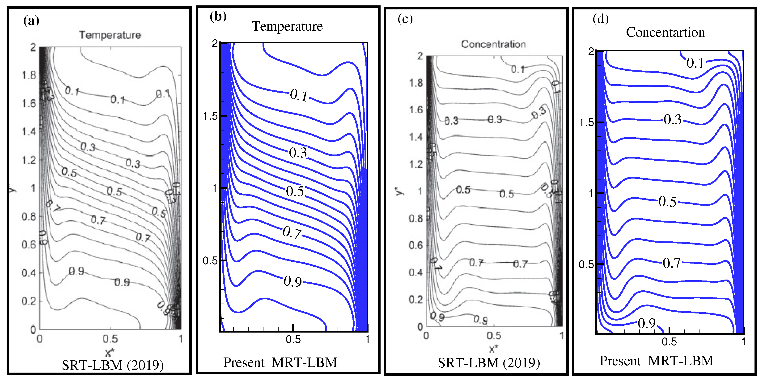
A qualitative comparison is shown in Figure 2 for the Soret and Dufour effects in terms of the isotherms and the isoconcentration lines obtained by Ren and Chan [37] using the single-relaxation-time (SRT) LBM while R a = 10 5 , P r = 1.0 , L e = 2.0 , S r = 0.1 , D f = 0.1 , B r = 10 , ϕ = 0.0 , ϵ = 1 and D a = 10 9 . By inspection, this qualitative comparison also confirmed the code validation.

5. Results and Discussion

The MRT-LB Simulation was applied to simulate the cross-diffusion natural convection of a nanofluid in a porous U-shape enclosure. The parameters specified here are the Rayleigh number, 10 4 R a 10 6 ; the volume fraction of the nanoparticle, 0.0 ϕ 0.04 ; the buoyancy ratio, 2 B r 2 ; the Darcy number, 10 4 D a 10 2 ; the Dufour number, 0 D f 0.2 ; the Soret number, 0 S r 0.2 ; and the Prandtl number, P r = 6.2 . In the velocity and temperature distribution, we vary the porosity, ϵ = 0.2 to 0.8 . The variant of the Lewis number, L e = 1 to 5, is also shown in N u ¯ and S h ¯ as a bar chart.

5.1. Observation of Streamlines, Isotherms and Isoconcentrations

Figure 3 represents the isotherms, streamlines, and isoconcentrations for various R a numbers and D a numbers at S r = 0 , B r = 1 , D f = 0.2 , ϵ = 0.4 , and ϕ = 0.0 (solid line), 0.04 (long-dashed line). The fluid responded by passing through the heated wall first, then the cold wall, moving upward and lower. For R a = 10 4 , 10 5 , and 10 6 , two vortexes were created on the left and heated right sides of the enclosure. The velocity changes across the vertical walls were greater than in the core zone of the left vortex, resulting in dense streamlines. Nevertheless, the concentrations were comparatively lower along the steep walls than in the middle area of the right vortex. The configurations of the streamlines and the isotherms were organized and distributed equally in all circumstances. The dimensions of the vortex grew rapidly as the R a numbers increased. The buoyancy effect caused the flow to circulate at the center of the enclosure and to descend along each side wall, creating mirror-image structures that revolved in the right and left half counter-clockwise. Both cells presented elliptical shapes. The symmetry ensured that the flows in the enclosure’s left and right halves were identical. As the fluid permeability across a cross-sectional area decreased, reduction in the D a number resulted in less buoyancy-induced flow, progressively thickening the boundary layer. The heat transfer decreased slightly as the R a number increased and the Darcy number decreased. The transfer of mass changed as shown in Figure 3g–i. A higher R a number and a lower D a number resulted in a synergistic rise in the mass exchange rate. The lower Darcy number complemented the higher flow velocity and convective transport generated by the higher R a number to produce a much more effective mass transfer process in the fluid.
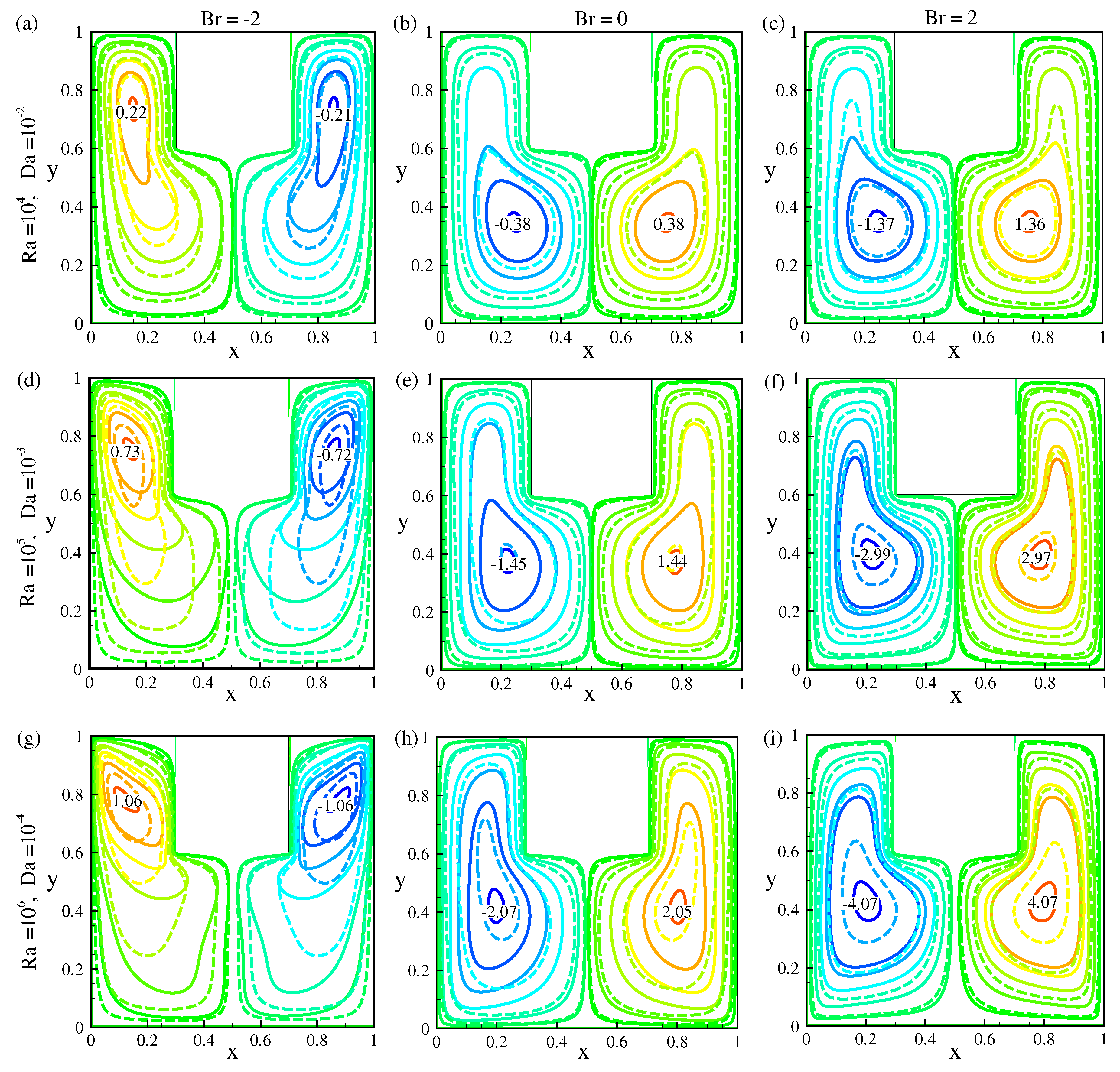
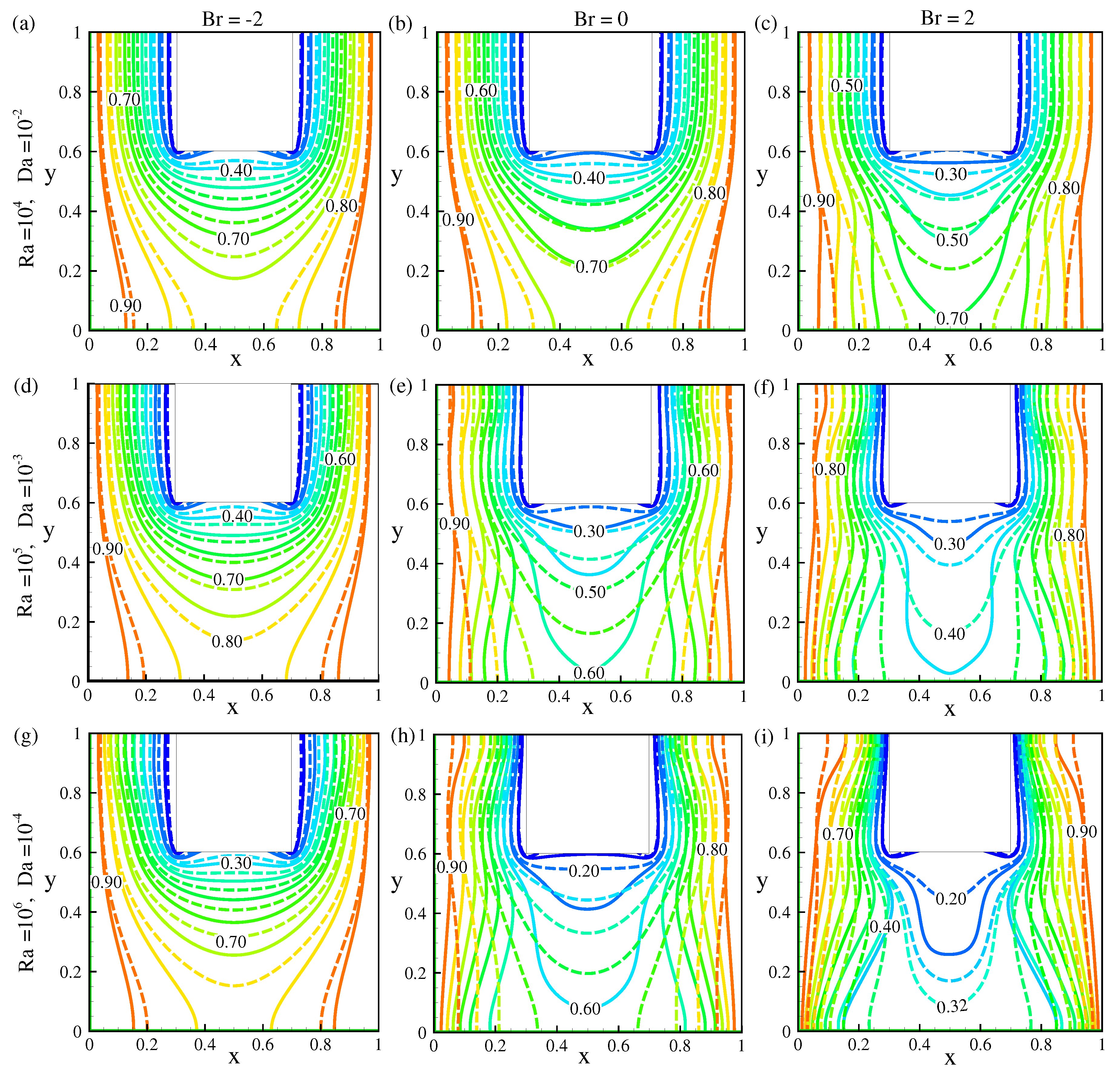
In addition, the buoyancy ratio was calculated using the density difference between the two fluids relative to their mean densities. This is essential for predicting and analyzing fluid behavior when the density differences are significant. The streamlines, isotherms, and isoconcentrations for the different buoyancy ratios with some fixed parameters are shown in Figure 4, Figure 5 and Figure 6. Two vortexes formed at the cavity’s upward portion in the streamline while the buoyancy force was opposing. The R a number is comparatively lower in Figure 4a–c. As the fluid flow increased, the flow structure became irregular due to the R a number’s augmentation and the reduction in the D a number, as shown in Figure 4d–i. The flow structure became erratic when the buoyancy force was applied from negative to positive due to the gravitational forces interacting with the density differences, leading to more pronounced and dominant buoyancy-driven convection. Positive buoyancy encourages vigorous fluid motion, making it a critical factor in natural convection, stratified flows, and other buoyancy-dominated fluid phenomena. Unsurprisingly, the most dominant fluid flow was observed when the R a number was at a maximum, and the buoyancy ratio was favorable, as shown in Figure 4i. As Figure 5 and Figure 6 show, the isotherms and isoconcentrations were consistent at opposing the buoyancy forces. The isoconcentrations and isotherm density close to the heated wall grew when the buoyancy force shifted from a negative to a positive value, indicating a rise in mass and heat transfer from the hot wall. Additionally, as the R a number and buoyancy ratio increased, the isotherms and isoconcentrations became more inconsistent.

5.2. Velocity and Temperature Effects

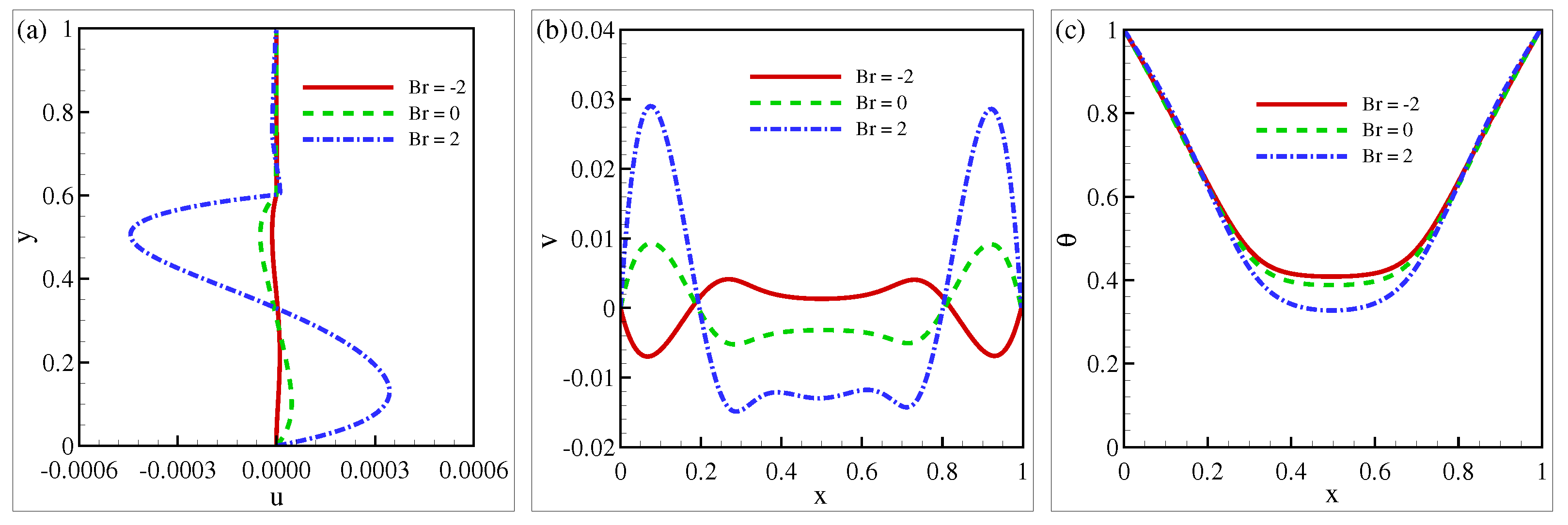
The changes in the velocity and temperature profiles under variable input parameters will be discussed here. In all cases, the u-velocity and the v-velocity will be represented along the x-axis and the y-axis, respectively, as shown in Figure 7a,b. The temperature profile along the y-axis for the different buoyancy effects (Br) is shown in Figure 7c. The other input parameters were as follows: R a = 10 4 , D a = 10 2 , D f = 0.2 , S r = 0.2 , ϕ = 0.04 and ϵ = 0.4 . Both the S r and D f impacts are present in this case. When the buoyancy effect was increased, the u-velocity grew in the region 0 < y < 0.3 but plummeted in the area 0.3 < y < 0.6 , as shown in Figure 7a, forming a symmetric shape. Unsurprisingly, the symmetrical shape was only visible at B r = 2 as the higher buoyancy influenced the proper velocity development. At y > 0.6 , the flow met the adiabatic wall of the cavity; hence, the fluid was immobile regardless of the B r values. Meanwhile, as per Figure 7b, the v-velocity went up rapidly at B r = 2 in the regions 0 < x < 0.2 and 0.8 < x < 1 . A similar pattern was observed at B r = 0 as well, but not as sharp as that of B r = 2 . However, as B r = 2 implied, the opposite pattern was observed regarding the v-velocity due to the negative magnitude of the buoyancy effect. In all cases, the symmetrical patterns were observed due to the symmetric configuration of a U-shaped cavity. Finally, the temperature distribution exhibited consistent patterns across all B r values, as shown in Figure 7c. The temperature distribution declined rapidly as the enhancing buoyancy ratio increased due to the buoyancy’s opposing force to the gravitational force. The strength of the buoyancy force grew relative to the gravitational force as the buoyancy ratio was augmented, resulting in a more consistent temperature distribution.
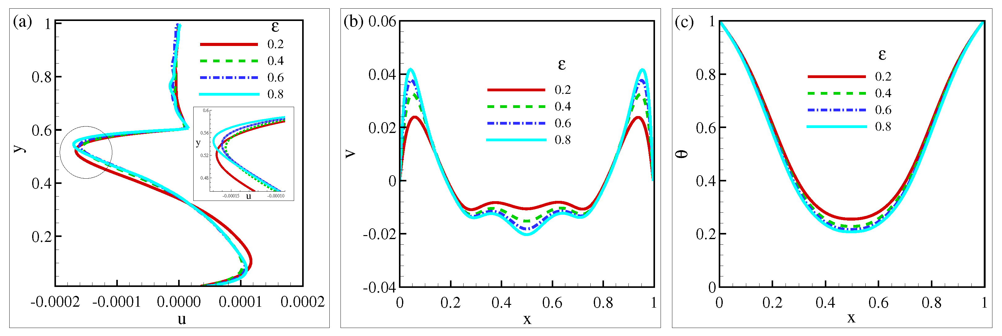
Figure 8 shows the temperature and the velocity distribution for the various porosities, ϵ ( 0.2 , 0.4 , 0.6 , 0.8 ), with some fixed parameters. The u-velocity increased with increasing porosity in the lowest half of the indicated circle but reduced in the upper half, as shown in Figure 8a. Meanwhile, as the rate of porosity increased, the v-velocity increased at both the heated walls but declined in the center of the cavity (Figure 8b). As the fluid attempted to pass through the restricted pathways that the increased density had generated, the flow resistance caused by the higher porosity closer to the heated walls caused a rise in the velocity. The higher pressure produced by the higher porosity caused this rise in velocity. Finally, the temperature distribution also decreased as the rate of porosity increased; this scenario was similar to that shown in Figure 8c. The temperature distribution decreased as the porosity increased due to increased friction within the system. As the fluid’s porosity increased, the interactions between its molecules became more intense, increasing the friction and heat release. As a consequence, the temperature gradient was diminished, causing a reduction in the temperature distribution.
Figure 9 describes the temperature and velocity distributions for varying nanoparticle volume fractions with some constant parameters, which are mentioned in the caption. The u-velocity declined with increasing volume fraction within the 0 < y < 0.3 region, but it increased in the 0.3 < y < 0.6 area, as shown in Figure 9a. According to Figure 9b, the v-velocity increased as a function of ϕ near the heated walls on the left- and right-sides. However, the velocity grew in the cavity’s center. Meanwhile, the temperature distribution shown in Figure 9c was diametrically opposed to that in Figure 7c and Figure 8c. In this case, the temperature distribution increased with rising ϕ . The increased number of molecules accessible to transfer energy improved the temperature distribution as the volume fraction increased. Since there were more molecules, more thermal energy raised the temperature as the volume fraction increased. As the number of molecules increases, a higher temperature gradient will result from more effective energy transfer.
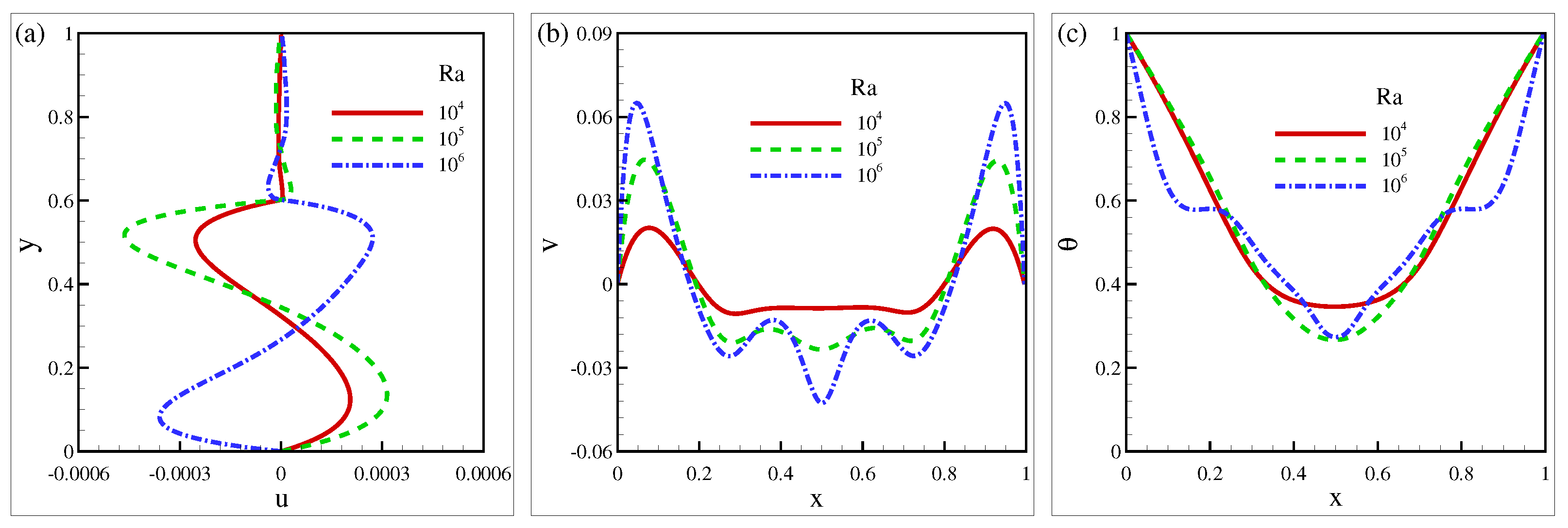
The effect of various R a numbers on the velocity and temperature distributions is depicted in Figure 10. In the region 0 < y < 0.3 , the u-velocity increased for R a = 10 5 , but decreased for a higher R a number at 10 6 . On the other hand, in the region 0.3 < y < 0.6 , the exact opposite scenario occurred. Here, the velocity decreased for R a = 10 5 but increased for R a = 10 6 . At R a = 10 5 , the buoyancy still did not fully dominate the flow. However, R a = 10 6 took over control of the velocity profile. In Figure 10b, the v-velocity increased near both the heated walls as the R a number increased. As the R a number augmented, the buoyancy forces became greater than the viscous forces, resulting in more freedom for fluid mobility. The increased fluid mobility led to high velocities near the heated walls. The temperature distribution was reduced as the R a number was augmented. The decreasing rate was greater at R a = 10 5 , but the decreasing rate was reduced when R a = 10 6 at the region 0.4 x 0.6 . As per Figure 10c, the temperature increased for R a = 10 5 and decreased for R a = 10 6 near the heated walls. In the region between 0.2 x 0.4 and 0.6 x 0.8 , the temperature distribution increased as the R a number increased.
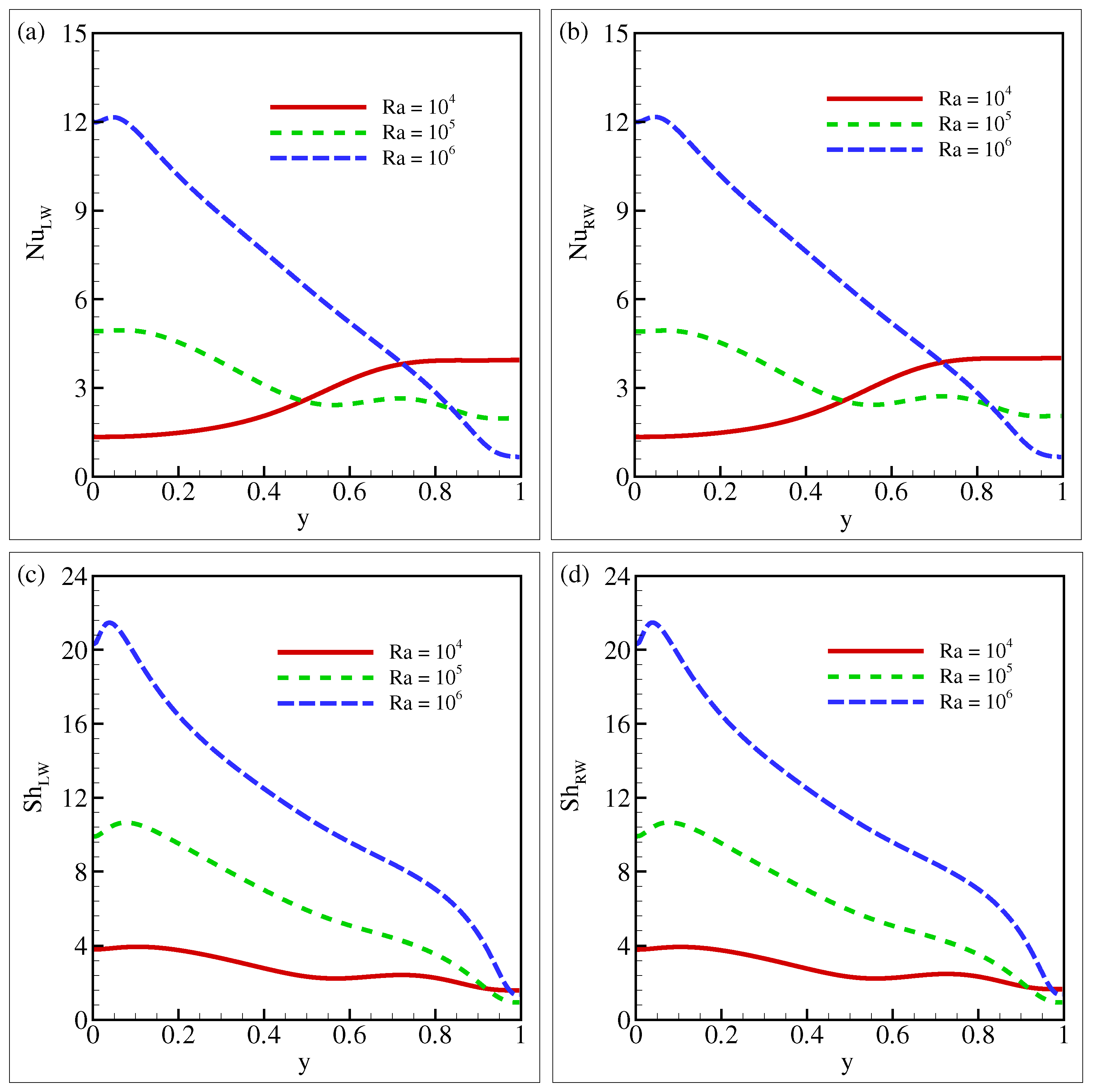
The local N u and local S h are illustrated in Figure 11 for different R a numbers when D a = 10 2 , D f = 0.1 , S r = 0.2 , B r = 1 , L e = 5 , ϕ = 0.04 , and ϵ = 0.4 . Figure 11a,c for the left wall, and Figure 11b,d for the right wall. It was observed that the N u and S h for the heated walls were quite similar. This indicated that the heat and mass transfers near both side walls were identical. When a fluid is heated from below during natural convection, it becomes buoyant and elevates while the colder fluid sinks. This circulation produces a convective flow pattern known as a thermal boundary layer. The R a number affects the flow pattern and the heat transmission properties. Unlike viscous forces, buoyant forces gain strength as the R a number rises. Convection cells inside the fluid grow more prominent and active as a consequence. These cells’ convective heat transfer enhancement produces a more significant convective heat transfer coefficient. As a result, increased values of the Nusselt numbers were observed in the area. Growth in the R a number also implied an excellent temperature differential across the fluid layer. The Nusselt number increased when there was a more significant temperature differential as it encouraged improved and efficient heat transfer rates. Consequently, the S h also increased with rising R a number, as presented in Figure 11c,d. The R a number, as previously stated, indicates the ratio of buoyant to viscous strengths and is not directly connected to the Sherwood number. Diffusion, rather than convection, is the principal driver of mass transfer in natural convection. The convective mass transfer coefficient is often substantially lower than the diffusive mass transfer coefficient. As a result, the Sherwood number is controlled more by the fluid’s diffusive features, such as the diffusion coefficient, than by the convective flow patterns associated with the R a number. Therefore, the local Sherwood number in natural convection is not directly affected by the rise in the R a number. However, it is essential to remember that when convective mass transfer becomes considerable, in some circumstances, modifications in the heat transfer and flow patterns features associated with variations in the R a number may indirectly impact the mass transfer rate and, subsequently, the Sherwood number.
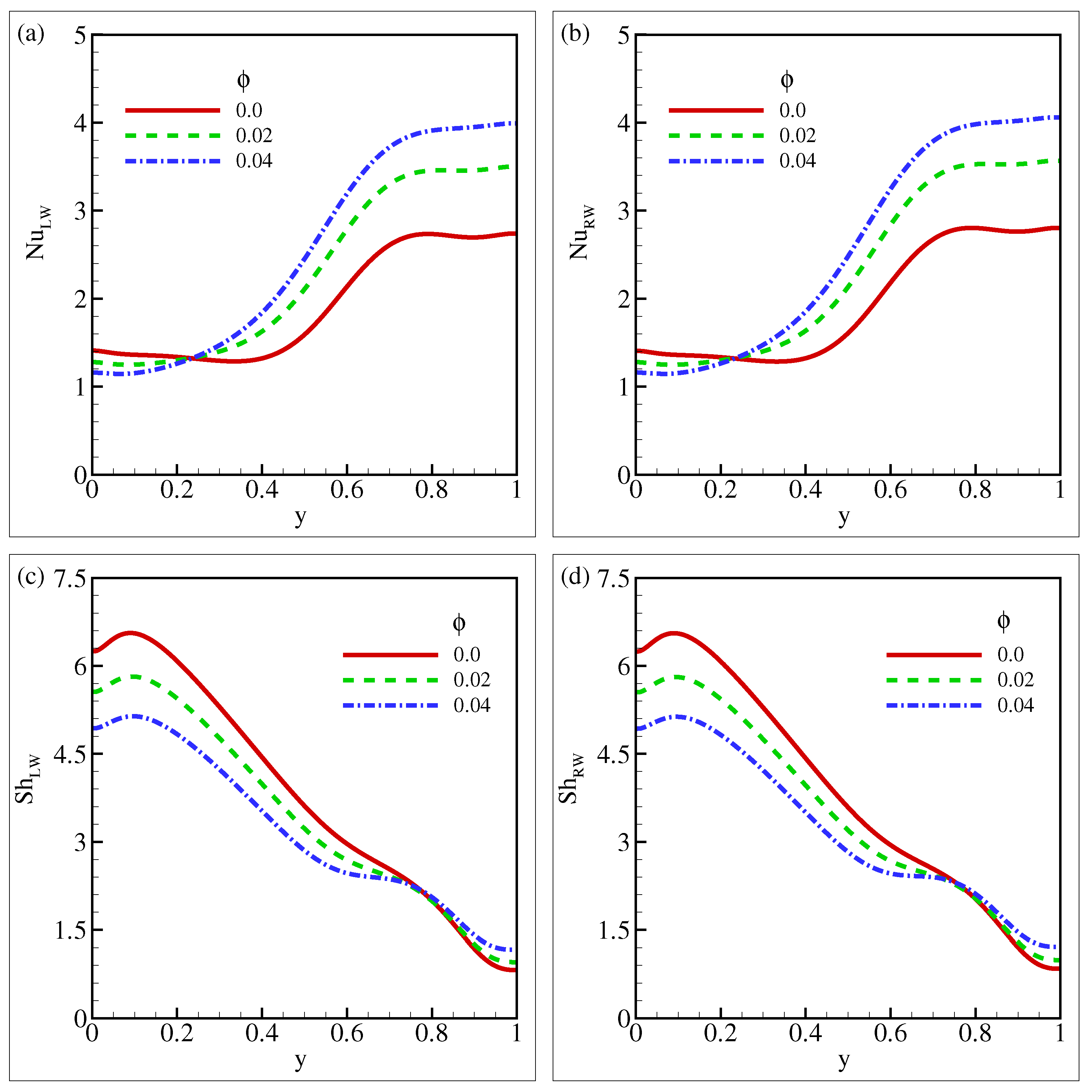
Figure 12 shows the local N u and local S h for various volume fractions. The N u reduces with rising volume fractions near the walls. Particle migration can occur when the volume proportion of particles close to the hot wall increases. This is because of the greater particle concentration on the heated surface, which might form particle-rich layers near the wall. The particles, which are usually less thermally conductive than the fluid, might behave as insulators, lowering the effective thermal conductivity of the combination. A lower N u was produced due to the decline in thermal conductivity, which hinders heat transfer from the heated border to the fluid. The scenario is opposite in the middle of the cavity. The local N u increased with an increasing volume fraction in that place. The local S h falls with enhancing the ϕ . A thicker concentration boundary barrier, decreased diffusivity, hindered fluid mixing, and concentration polarization can all result from an increased particle or solute volume fraction. These elements work together to lower the local Sherwood number, which denotes a slower mass transfer rate as the volume fraction rises. Considering these drawbacks, while optimizing the flow conditions, mixing techniques, and concentration gradients, is critical to increasing the mass transfer efficiency in such situations.

5.3. Mean Nusselt Number ( N u ¯ ) and Mean Sherwood Number ( S h ¯ ) for Different Parameters

The N u ¯ and the S h ¯ for different R a numbers, D a , and S r are shown in Table 6. It was found that the N u ¯ decreased as the flow became more laminar, and the fluid velocity dropped as D a decreased. The equation of D a represents the flow regime in a porous medium. Consequently, the N u ¯ also dropped as the convective heat exchange factor dropped. The N u ¯ increased with increase in the R a number. As R a increased, the fluid flow experienced more mobility due to improved strength in the buoyancy that enhanced the heat transfer. The ratio of the convective heat transfer acceleration to the conductive heat transfer rate determines the N u ¯ , which increases with increasing R a numbers since the convective heat transfer rate rises with more significant fluid motion. The variations in N u ¯ were significantly lower as the S r increased. The S h ¯ increased as the S r increased. The S r number indicated a rise in the concentration gradient, which suggested a rise in the diffusivity. The concentration gradient and the diffusivity were related to the Sherwood and Soret numbers of the transferred species. The S h ¯ also increased with increase in the R a numbers and decreased as the Darcy number decreased.
In Table 7, the N u ¯ and the S h ¯ are displayed for the various Dufour numbers ( D f = 0 , 0.1 , 0.2 ), ϕ = 0.0 , 0.02 , 0.04 , and B r = 2 , 0 , 2 from a quantitative perspective. It can be seen that the N u ¯ increased as the ϕ increased as the particles were more thermally conductive. The addition of nanoparticles improved the nanofluid’s overall thermal conductivity. It was observed that when the buoyancy ratio varied from negative to positive for D f = 0 and ϕ = 0.0 , the ( N u ¯ ) increased by 82.03 % . Furthermore, in the case of D f = 0.1 and D f = 0.2 for ϕ = 0.0 , the ( N u ¯ ) was enhanced by 81.37 % and 80.59 % , respectively. The acceleration of growth decreased as the ϕ increased. As ϕ increased from 0 to 0.04 for D f = 0 and B r = 2 , the N u ¯ was reduced by 5.38 % . At B r = 2 , the decreasing rates were 7.90 % and 8.79 % , respectively, when D f = 0.1 and D f = 0.2 . On the other hand, the same scenario occurred for the S h ¯ . The S h ¯ increased with enhancement in the buoyancy ratio. This could be explained by the fact that as the buoyancy forces grew more powerful than the diffusion forces, the convection mechanism became more dominant in the mass transfer. It can be observed that the S h ¯ declined as the ϕ increased, but when D f = 0.2 and B r = 2 , the S h ¯ rose. The fluid movement faced more restriction with increased ϕ , and the mass transfer rate plummeted concurrently.
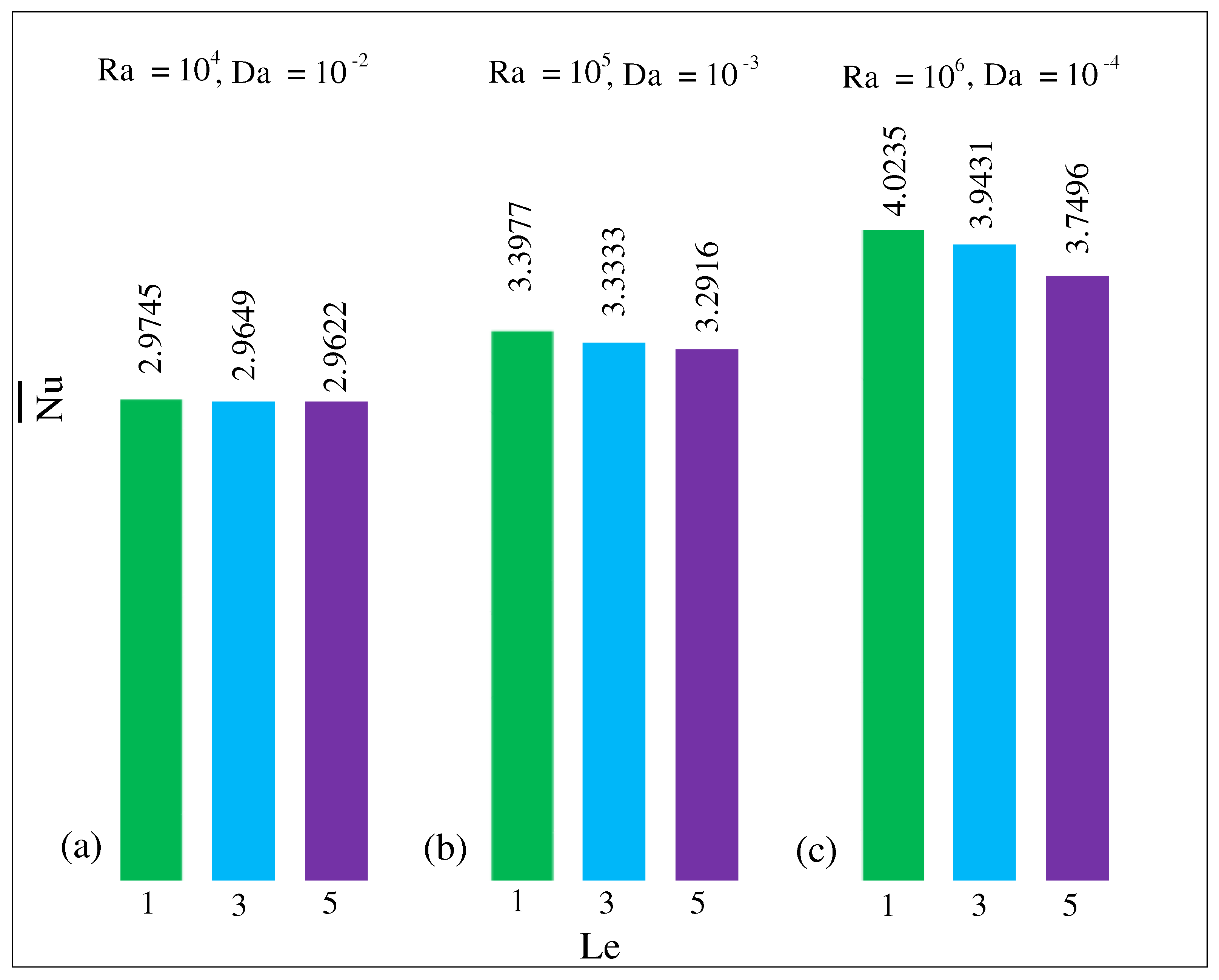
The N u ¯ against various Lewis numbers for different R a numbers and Darcy numbers with some constant parameters is shown in Figure 13. It was observed that the N u ¯ decreased as the Lewis number increased. However, as the D a numbers decreased and the R a numbers increased, the N u ¯ increased. In Figure 13a, the decreasing rate of the N u ¯ was 0.41 % for L e = 1 to 5. For higher values of the L e number, less heat will transfer across the cavity due to increasing convective motion. The L e number increased, meaning more convection than conduction occurred in the enclosure. As L e increased, the N u ¯ dropped as less energy could be transported from one area to another by conduction than if only convection were in effect. Similarly, the rate of N u ¯ decreased by 3.12 % and 6.81 % in Figure 13b,c, respectively. It was observed that the reduction rate increased as the D a and R a numbers increased. The N u ¯ increased with increase in the R a numbers, and the N u ¯ increased as the D a numbers decreased due to enhanced convective heat transfer. As the D a numbers decreased and the R a numbers increased, more energy was forced into the system, causing an increase in the fluid motion due to the thermal buoyancy forces. The N u ¯ augmented 14.23 % , when the value of D a = 10 2 and R a = 10 4 changed to D a = 10 3 and R a = 10 5 while L e = 1 .
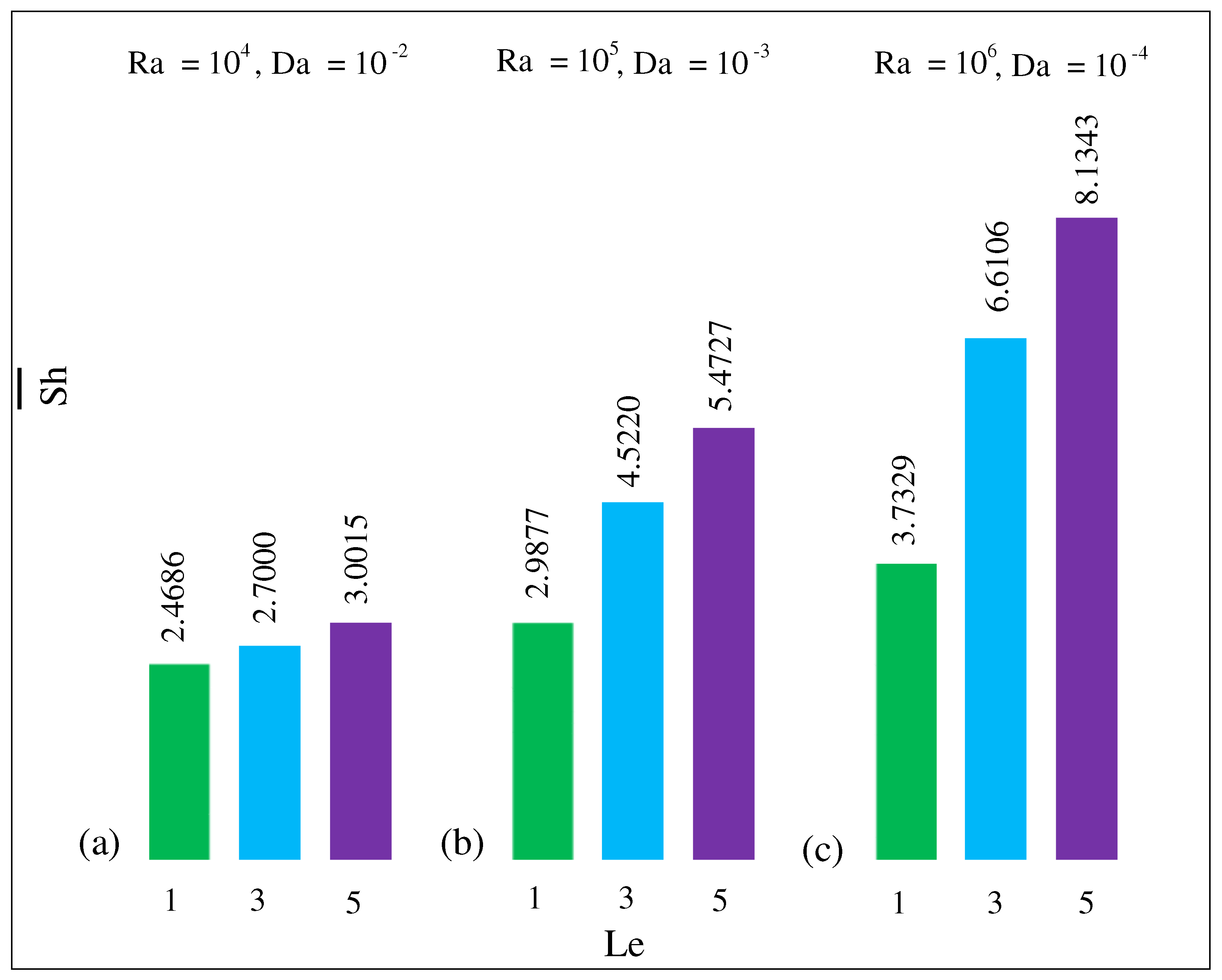
In the last part of this segment, Figure 14 depicts the S h ¯ against various Lewis numbers for different R a and Darcy numbers with some fixed parameters. The S h ¯ increased with progress in the L e . The S h ¯ increased 20 % when the L e increased from 1 to 5 in Figure 14a. The increasing rates were 83.17 % and 117.90 % , as shown in Figure 14b,c. As the number of R a increases, so does the S h ¯ . As the number of D a decreases, S h ¯ increases. The S h ¯ was highest for L e = 5 when the D a numbers were lower and the R a numbers were higher. The S h number is the convective and diffusive mass transfer ratio. It indicates the convective heat transfer performance and is usually proportional to the L e . Increasing the L e (thermal diffusivity ratio to mass diffusivity) in a nanofluid-filled porous enclosure caused the diffusive mass transport to become relatively slower than the convective mass transport. This caused the S h to rise as the Lewis number increased. When D a = 10 2 and R a = 10 4 increased to D a = 10 4 and R a = 10 6 for L e = 5 , the mean Sherwood number augmented to 174.6 % .

5.4. Entropy Generation

Entropy is a measurement of the disorder or unpredictability of a technique, and it is produced naturally due to irreversible processes. Table 8 shows the entropy generation with varying parameters while some parameters were kept constant. In general, the entropy generation due to fluid friction M F increases as the R a number increases but reduces as the volume fraction of the nanoparticles increases. Fluid friction in natural convection tends to rise as the R a numbers do. This could be explained by the fact that at higher R a numbers, the forces generated by buoyancy outweigh the strengths driven by viscosity, resulting in more dominant fluid mobility and stronger convective currents. As the fluid passes over solid surfaces or through porous media, these more significant currents increase the frictional resistance. The fluid friction lowers as the volume percentage of the solid particles in the fluid rises; the solid particles are mostly responsible for this phenomenon. The solid particles obstruct the flow of fluid as the volume fraction rises. As an impact, the overall fluid velocity decreases, and the flow distribution becomes spontaneous due to the reduced fluid friction. As per Table 8, the heat transfer increased for R a = 10 4 and R a = 10 5 but decreased for 10 6 as ϕ increased. After 4 % of the volume fraction was included, the mass transfer decreased by 16.22 % , 15.85 % , and 14.49 % , while the Rayleigh number was assigned 10 4 , 10 5 , and 10 6 , respectively, for D f = 0.0 . As the Dufour number increased, the mass transfer also increased. The M S increased with increase in the R a numbers but decreased with increasing ϕ , while R a = 10 5 and 10 6 . For all cases, the mean Bejan numbers ( B e a v g ) were always greater than 0.5 , which indicated that irreversibility became dominant due to heat transfer.
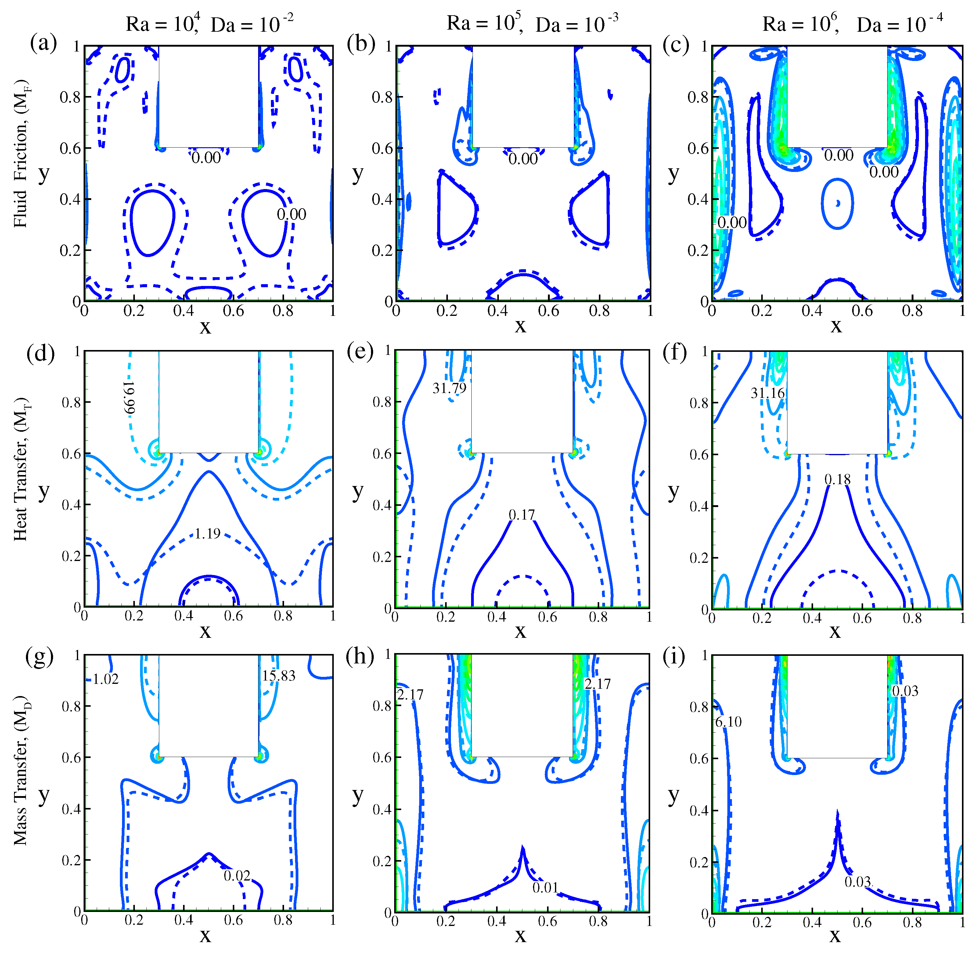
The entropy generation due to fluid friction, ( M F ) , heat transfer ( M T ) and mass transfer ( M D ) in a u-shaped porous enclosure for various Rayleigh and Darcy numbers while S r = 0.2 , D f = 0.2 , B r = 1 , P r = 6.2 with ϕ = 0.0 (solid line) and 0.04 (dashed line) are shown in Figure 15. The entropy formation from fluid friction rises as the Rayleigh and Darcy numbers, respectively, rise and fall. The maximum entropy is produced near the heated walls and the cold part of the u-shaped porous enclosure when D a = 10 4 and R a = 10 6 in Figure 15c. Figure 15d–f illustrates the entropy generation due to M T . The M T increases as the Rayleigh and Darcy numbers increase, respectively. The maximum M T occurs near the upper cold wall of the enclosure when D a = 10 4 and R a = 10 6 . Natural convection happens when temperature differences in a fluid cause density variations. When a fluid is heated, its density reduces, causing it to become lighter and rise. The more beneficial fluid, on the other hand, grows denser and sinks. This circulation culminates in the production of convection cells, which are patterns of convective movement. The R a number substantially influences the heat transfer rate in natural convection. When the R a number grows, the buoyant forces precede the viscous forces. As an outcome, the convective flow becomes more significant and noticeable. With enhanced fluid velocity, faster-moving convection cells correspond to higher Rayleigh numbers. The increased fluid velocity ensures that heat is transported faster throughout the system. The M D is found to rise when the Rayleigh and Darcy numbers grow and decrease, respectively. After adding the 4 % volume fraction, the M F decreases by 38.46 % , the M T increases by 55.85 % , and the M D increases by 11.81 % for D a = 10 2 and R a = 10 4 . For D a = 10 3 and R a = 10 5 , the M F decreases by 26.53 % , the M T increases by 35.89 % , and the M D decreases by 16.05 % . Similarly, the fluid friction decreases by 22.34 % , the M T rises by 21.34 % , and the M D reduces by 15.14 % when R a = 10 6 and D a = 10 4 .
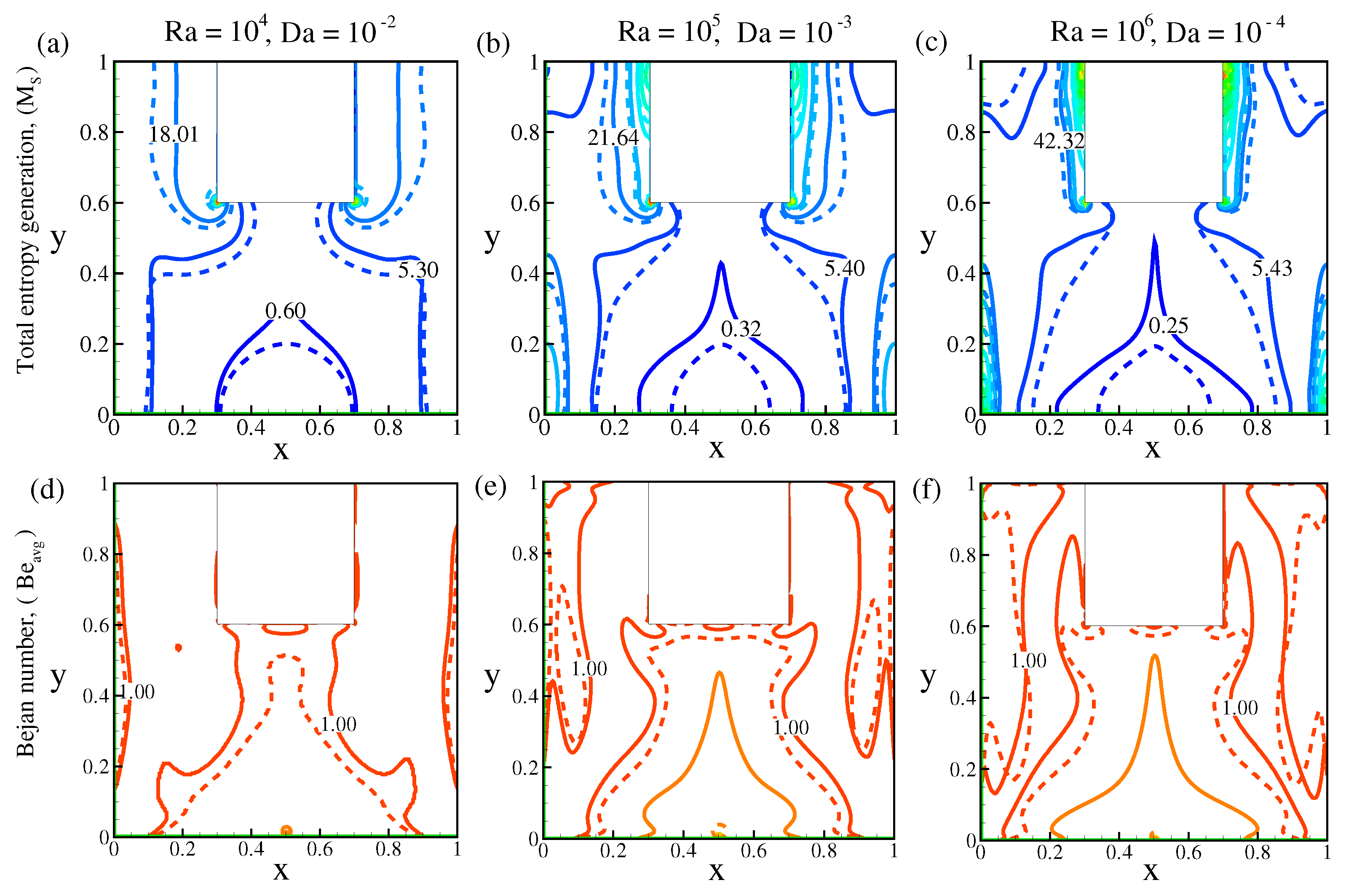
Figure 16 demonstrates the M s and the mean B e a v g number for various R a numbers and Darcy numbers for S r = 0.2 , D f = 0.2 , B r = 1 , P r = 6.2 with ϕ = 0.0 (solid line) and ϕ = 0.04 (dashed line). The M s increases as R a and D a rise and fall. Higher Rayleigh numbers are associated with more muscular buoyancy motion of the fluid, leading to increased irreversibility and energy dissipation within the system. Entropy creation measures a system’s irreversibility or loss of accessible energy. In any real-world process, there are always inefficiencies that lead to the generation of entropy. Entropy creation occurs due to irreversible processes, such as heat transfer across temperature gradients, viscous dissipation, and other dissipative effects. Overall, the combined effects of enhanced viscous dissipation within the fluid and increased entropy generation at the solid–fluid interface result in higher total entropy generation in the system as the Rayleigh number grows. The total entropy generation increases by 27.52 % for R a = 10 4 , D a = 10 2 , 8.19 % for D a = 10 3 , R a = 10 5 , and 0.48 % for D a = 10 4 , R a = 10 6 , after adding the 4 % volume fraction. The B e a v g is almost constant as the Rayleigh and Darcy numbers rise and fall, respectively. From this finding, the B e a v g is higher than 0.5, which indicates that the irreversibility becomes heat transfer dominant.

6. Response Surface Methodology

A response surface methodology (RSM) is a statistical and mathematical process for modeling and optimizing the connection between numerous independent variables (factors) and a response (dependent variable). It is frequently used in experimental design and analysis to strengthen, enhance, and comprehend intricate systems or processes. RSM uses mathematical models to approximate the link between the independent factors and the response. Higher-order models may also be utilized depending on the system’s complexity, while second-order polynomials are frequently used to express these models. RSM aims to identify the independent variables’ ideal values that produce the best or desired response. Maximizing, decreasing, or setting the reaction to a particular target value is possible. RSM aids in locating and calculating how the independent variables interact with one another. This is essential for comprehending the system’s behavior and determining how different variables affect the response.
Here, R 2 = 99.81 , adjusted R 2 = 99.43 , and predicted R 2 = 93.03 % . In this RSM section, there were five parameters taken as variables, where 10 4 R a 10 6 , 0.0 D f 0.2 , 1 B r 1 , 0.0 S r 0.2 and 0.0 ϕ 0.06 were considered for this correlation analysis. The other parameters P r = 6.2 , L e = 5 , ϵ = 0.4 and D a = 10 2 were kept constant for this correlation, as shown in Equation (79).
N u ¯ = 2.05031 + 6.28 × 10 6 R a + 2.9009 D f + 0.044483 B r + 1.36280 S r + 26.27675 ϕ + 3.13 × 10 6 R a D f + 9.34 × 10 7 R a B r 2.13 × 10 6 R a S r 0.000015 R a ϕ + 0.534527 D f B r 21.76136 D f S r 62.26668 ϕ D f + 1.01756 B r S r 2.84153 B r ϕ + 6.78964 S r ϕ 2.11 × 10 12 R a 2 + 23.16652 D f 2 0.305389 B r 2 + 8.19961 S r 2 201.00616 ϕ 2
In Table 9, the model is essential given its standard F-value of 261.81 . A value of F this large might occur due to noise just 0.01 % of the time. When the p-value for a model term is less than 0.05 , it is deemed significant [48]. In this case, the essential model terms are R a , D f , B r , R a × D f , R a × B r , R a × S r , R a × ϕ , D f × S r , D f × ϕ , B r × S r , R a 2 , D f 2 , B r 2 , and ϕ 2 . The model terms are not considered significant if the value exceeds 0.1000 . Model reduction may improve a model if it contains a lot of unnecessary words (except those needed to maintain hierarchy). The lack of fit F-value of 180.98 showed the significance of the lack of fit. An elevated lack of fit F-value has a 0.01 % chance of being brought on by noise. To describe the relation between the response function and the input factors ( R a , D f , S r , B r , and ϕ ), consider the following mathematical connection:
N u ¯ = 2.05031 + 6.28 × 10 6 R a + 2.9009 D f + 0.044483 B r + 3.13 × 10 6 R a D f + 9.34 × 10 7 R a B r 2.13 × 10 6 R a S r 0.000015 R a ϕ 21.76136 D f S r 62.26668 ϕ D f + 1.01756 B r S r 2.11 × 10 12 R a 2 + 23.16652 D f 2 0.305389 B r 2 201.00616 ϕ 2

Response Surface Analysis

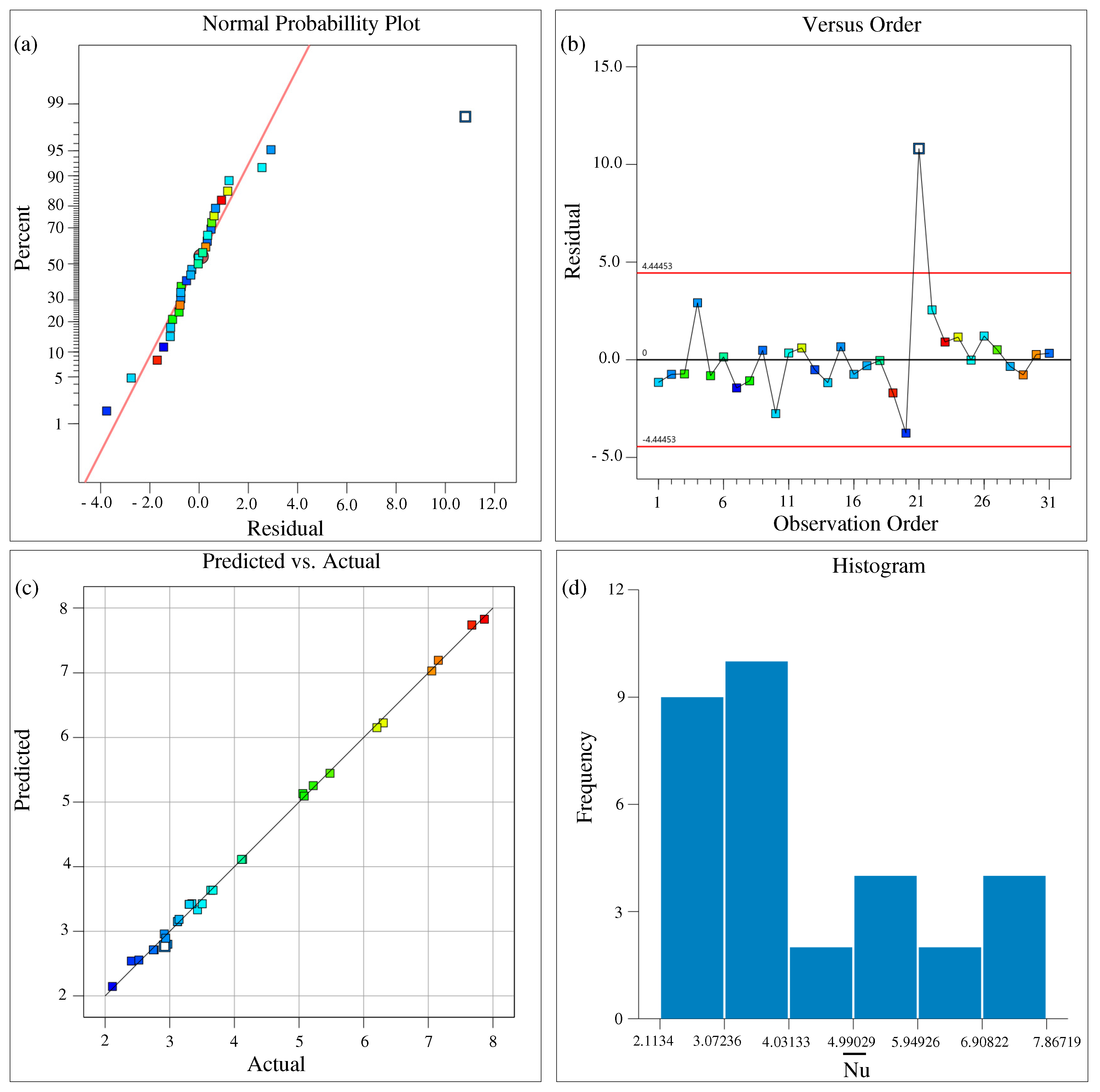
Figure 17 shows four different residual plots developed after entering the data into statistical software and performing a variance analysis (ANOVA). The degree of accuracy of fit in regression is measured using the residual graphs. The residuals in Figure 17a show the standard probability plots were very acceptable. Locating any predictable biases in the model is aided by a percent-versus-residual graph. It can reveal over-prediction or under-prediction in a variety of operational circumstances. Over-prediction is the positive percentage of errors, and under-prediction is the harmful percentage. It gives an impression of the regions where the model must be improved or changed to increase accuracy. Figure 17b displays the residual versus the observation plot. The regression model performance can be assessed using this graph, which shows the residuals against the order of the observations. Using the residuals can assist in identifying patterns and trends that can enhance the model or identify data problems. This graph’s main objective is to look for regular patterns or correlations in the residuals caused by the data’s temporal order. The residuals should have a random distribution centered on zero to demonstrate the model’s accuracy and be unaffected by the data recording order. Residuals that change in magnitude as the observations progress indicate a systematic trend or an inaccuracy in the model’s estimates. This pattern implies that the model should consider any sequential or temporal elements that impact N u ¯ . Looking for outliers or sudden modifications in the residuals at specific statement sites can help detect a clear difference between the expected and the actual values. To enhance the N u ¯ forecast’s accuracy, the model may require updating, considering additional variables, or acknowledging temporal dependencies. For all the responses in our simulation, we observed that the most significant residuals for N u ¯ were close to 11.5 . The difference between the expected and actual results for N u ¯ is seen in Figure 17c. Analyzing the predicted vs. accurate graph will determine the prediction system’s dependability and accuracy. The residuals were found to be close to or on a straight line, demonstrating the regression models’ accuracy in fitting the data. The typical probability plots of the residual distributions are shown to evaluate the observation’s normality. Given that this line is straight, the N u ¯ residual distribution is assumed to be predictable. Figure 17d shows an irregular distribution of the residual histograms that does not approximate a symmetrical distribution. The frequency initially rises to 4.03133 and then falls. Between 4.99029 and 5.94926 , the frequency again rises. After increasing the frequency, it again reduces with increase in N u ¯ . The maximum frequency was observed between the N u ¯   3.07236 and 4.03133 .
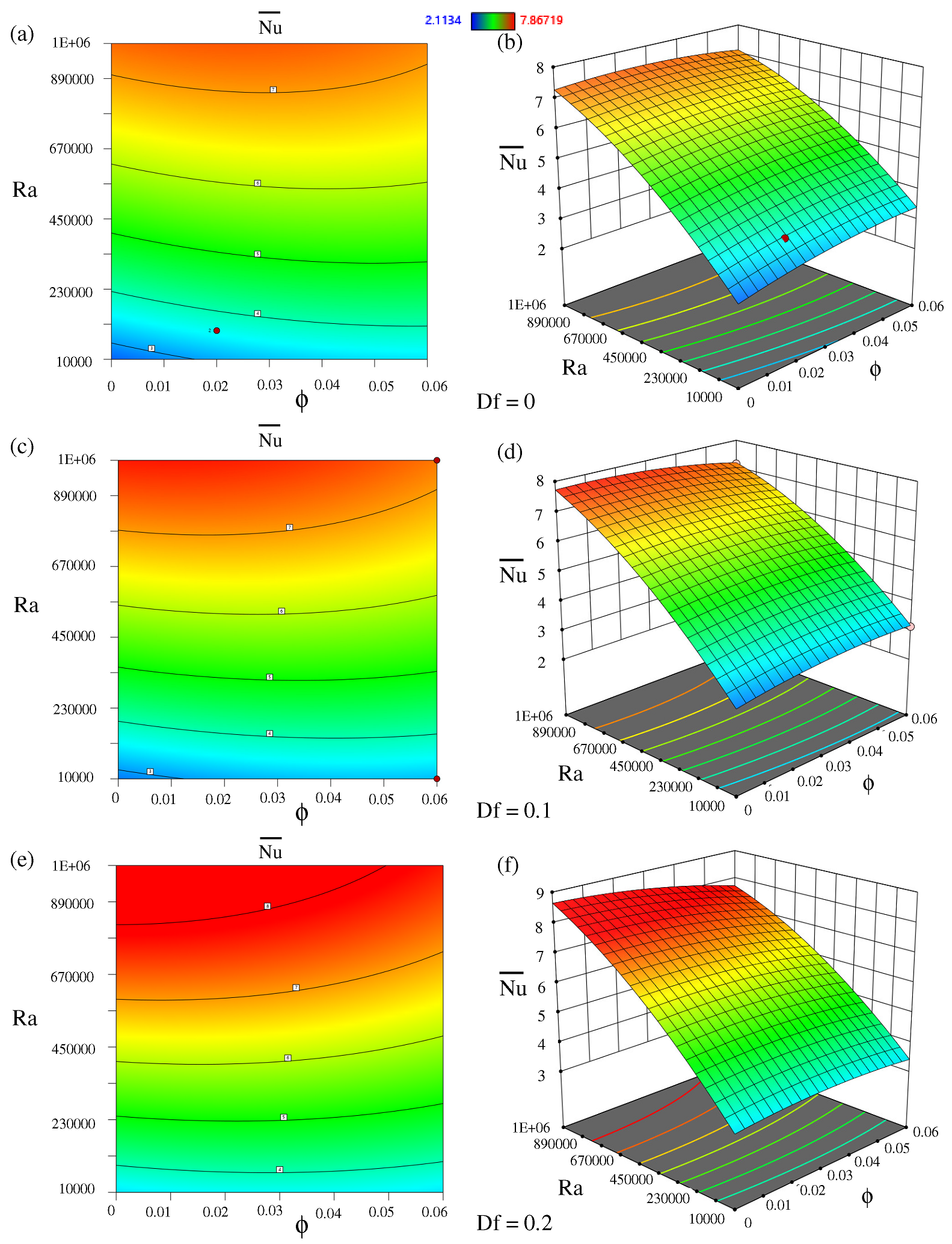
A mathematical model or outline plot is a two-dimensional visible representation of result variables as a process involving two separate factors. The response surface plotting functions are similar to 3D character plotting but present the response variable as a collection of contour lines in a 2D texture. A model contour plot displays the independent variables on the x- and y-axes, while a series of contours represents the response variable. The model contour and response surface plots for illustrating the impact of various self-dependent factors on N u ¯ are shown in Figure 18.
The response function N u ¯ with R a and ϕ for various Dufour numbers is shown in Figure 18 with some fixed parameters. The relationship between R a and ϕ for the response function N u ¯ is analyzed through 2D and 3D graphs, maintaining constant D f . These 2 D and 3 D graphs indicate that the N u ¯ is maximum at the highest R a number, and as the ϕ increases, the N u ¯ also increases. The system’s improved convective heat transfer indicates superior buoyancy-driven forces over conduction and increased heat exchange interfaces due to higher volume fractions. The N u ¯ was slightly higher as the D f increased.

7. Sensitivity Analysis

Sensitivity analysis in the natural convection of nanofluids refers to systematic research on how modifications to various parameters and variables might impact the heat transfer characteristics of a nanofluid (a fluid containing nanoparticles). Understanding the effects of uncertainties and fluctuations in the input parameters on the system’s output is made possible using this helpful instrument in scientific study and engineering. Researchers and engineers may make wise design and application decisions using sensitivity analysis to better understand the nanofluid’s behavior and to improve its performance, and to pinpoint the essential elements that significantly impact the nanofluid’s natural convection heat transfer mechanism. These variables might be the kind and quantity of nanoparticles, the fluid characteristics (like the viscosity and the thermal conductivity), the size and form of the heated surface, the boundary conditions (like the temperature gradients), and the external variables (like gravity). Sensitivity analysis involves purposefully changing certain factors one at a time while leaving the others constant. Possible real-world values or extreme scenarios may be included in the range of variation. Researchers may, for instance, vary the thermal conductivity of the fluid, the concentration of the nanoparticles, or the temperature differential across the heated surface. A sensitivity analysis examines how parameter changes affect the heat transfer properties, including the temperature distribution in the nanofluid, the convective heat transfer coefficient, and the heat transfer rate. This procedure aids in determining which variables significantly affect how the system behaves. Individual partial derivatives of the dependent variable ( N u ) concerning the independent variables R a , D f , B r , S r , and ϕ are calculated in this work. We were able to obtain the intended results by considering the values of the independent components at three levels: 1 (low), 0 (medium), and 1 (high). The sensitivity is calculated using the regression Equation (80). The partial derivative of the function that produces the result ( N u ¯ ) concerning the independent variables is used to determine the sensitivity. The response function’s sensitivity functions are as follows:
N u ¯ R a = 6.28 × 10 6 + 3.13 × 10 6 D f + 9.34 × 10 7 B r 2.13 × 10 6 S r 0.000015 ϕ 4.22 × 10 12 R a
N u ¯ D f = 2.9009 + 3.13 × 10 6 R a 21.76136 S r 61.26668 ϕ + 46.33304 D f
N u ¯ B r = 0.044483 + 9.34 × 10 7 R a + 1.01756 S r 0.610778 B r
N u ¯ S r = 2.13 × 10 6 R a 21.76136 D f + 1.01756 B r
N u ¯ ϕ = 0.000015 R a 62.26668 D f 402.01232 ϕ
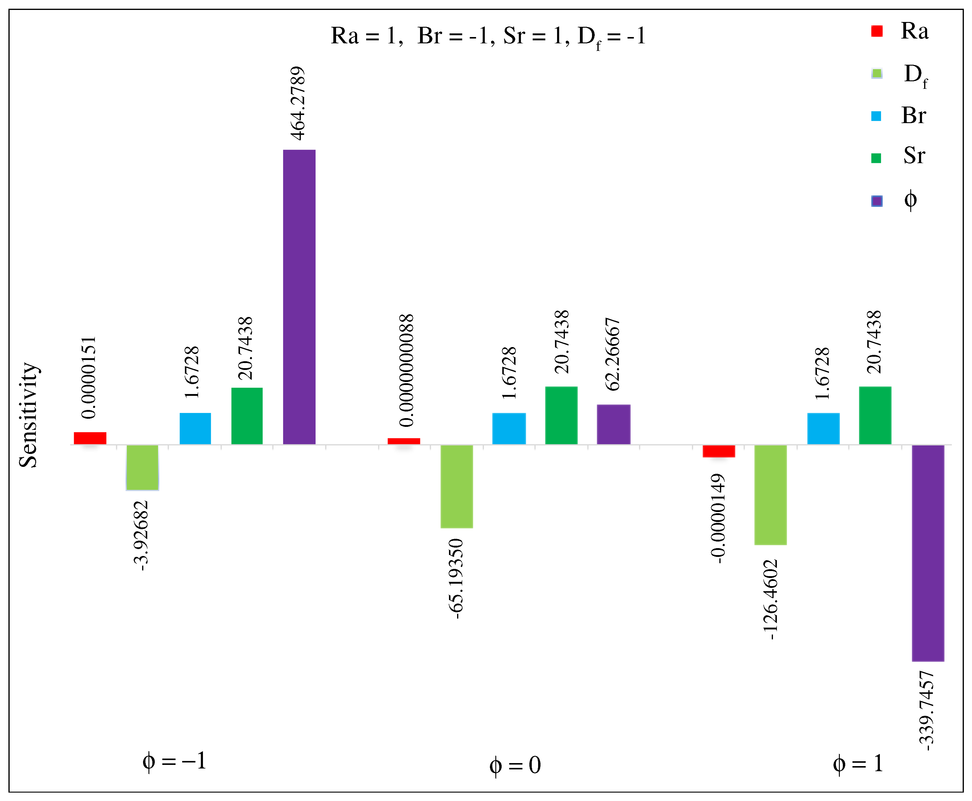
A positive sensitivity output indicates that increasing the input variable’s value improves the output operation’s value. A negative sensitivity value also indicates a decrease in the output factor caused by increasing the input factor. The sensitivity analysis for various R a , D f , B r , S r and ϕ quantities on the output response N u is shown in Table 10 and Figure 19. It was observed that the sensitivity metrics of R a and ϕ were positive when the volume fraction value was the lowest or medium. However, the sensitivity was negative when the volume fraction was the highest. and positive sensitivity was observed for B r and S r . When the Soret number is raised, the Soret effect becomes more significant than thermal diffusion. In some cases, increasing the Soret number can result in improved separation or concentration gradients of the mixture components, resulting in higher heat and mass transfer rates. This can lead to positive sensitivity, where increasing the Soret number enhances the total transport efficiency. Increasing the buoyancy ratio can lead to stronger natural convection currents in the fluid. This increased fluid motion can improve the heat and mass transfer rates, resulting in positive sensitivity. D f has a positive sensitivity when the S r is medium; otherwise, in all cases, the sensitivity of D f is negative.

8. Conclusions

The study explores the impact of the Dufour and Soret effects on the thermosolutal natural convection of a Newtonian A l 2 O 3 - H 2 O nanofluid in a U-shaped porous enclosure. Varying parameters were investigated in the study: the Rayleigh number ( R a = 10 4 , 10 5 , 10 6 ), the Darcy number ( D a = 10 2 , 10 3 , 10 4 ), the Soret number ( S r = 0.0 , 0.1 , 0.2 ), the Dufour number ( D f = 0.0 , 0.1 , 0.2 ), the buoyancy ratio ( 2 B r 2 ), the Lewis number ( L e = 1 , 3 , 5 ), the volume fraction ( 0 ϕ 0.04 ), and the porosity ϵ = ( 0.2 0.8 ). The numerical findings were represented in graphical and tabular form to provide quantitative and physical information regarding the generated solutions. The RSM provided the 2D contour and 3D surface plots that are displayed. The RSM method was also used to investigate the sensitivity of the N u ¯ to the input parameters. The following are the principal findings of this study:
  • The fluid flow is enhanced as the Rayleigh number and buoyancy force increase. The isotherm and isoconcentration densities close to the hot wall grow when the buoyancy force shifts from a negative to a positive value.
  • The u-velocity at mid-x rises between 0 y 0.3 but decreases between 0.3 y 0.6 by growing the B r . The v-velocity at mid-y enhances close to the walls and reduces in the middle of the cavity for rising B r and ϵ . The temperature distribution also decreases by increasing B r and ϵ .
  • The v-velocity at mid-y decreases near the walls but enhances at the down-indented part of the U-shape with increasing ϕ . The temperature distribution rises as the ϕ rises.
  • The temperature distribution at the down-indented portion of the U-shape and the v-velocity at mid-y decrease as the R a number rises. But they increase close to the walls as the R a number rises.
  • The local N u and the local S h increase as the R a number rises but reduce as the volume fraction increases.
  • The N u ¯ and S h ¯ decrease as the Darcy number falls, but both rise as the R a number increases. The N u ¯ and the S h ¯ rise as the buoyancy ratio shifts from a negative to a positive value.
  • As the L e number reduces, the N u ¯ reduces, but the S h ¯ rises.
  • The fluid friction M F rises as the R a number rises, but reduces as the volume fraction rises. The heat transfer M T increases for R a = 10 4 and 10 5 , but decreases for R a = 10 6 as the volume fraction rises.
  • The B e a v g is always more than 0.5 , which indicates the irreversibility becomes heat transfer dominant.
  • The generated correlation equation from the RSM approach demonstrates the correlation between the output and the input parameters.
  • The B r and S r have a positive sensitivity, but R a and ϕ have a negative sensitivity only for higher values of ϕ .

Author Contributions

Conceptualization, M.M.I. and M.M.M.; methodology, M.M.I. and M.M.M.; software, M.M.I. and M.M.M.; validation, M.M.I. and M.M.M.; formal analysis, M.M.I. and M.F.H.; investigation, M.M.I., M.F.H. and M.M.M.; resources, M.M.I., M.F.H. and M.M.M.; data curation, M.M.I. and M.M.M.; writing—original draft preparation, M.M.I. and M.F.H.; writing—review and editing, M.F.H. and M.M.M.; visualization, M.M.I., M.F.H. and M.M.M.; supervision, M.M.M.; project administration, M.M.M.; funding acquisition, M.M.M. All authors have read and agreed to the published version of the manuscript.

Funding

The last author (M.M.M.) gratefully acknowledges the North South University for the financial support as a faculty research grant (Grant No.: CTRG-23-SEPS-11). The last author also acknowledges the Ministry of Science and Technology (MOST), Government of Bangladesh, for providing the financial support for this research (Grant No.: EAS/SRG-222427).

Data Availability Statement

The data are available by request.

Conflicts of Interest

The authors declare no conflict of interest.

Abbreviations

The following abbreviations are used in this manuscript:
Abbreviations
ANOVAAnalysis of variance
BFEDMBrinkman–Forchheimer extended Darcy model
FEMFinite element method
FVMFinite volume method
LBMLattice Boltzmann method
MHDMagnetohydrodynamics
MRTMultiple-relaxation-time
RSMResponse surface methodology
Nomenclature
English symbols
B e Local Bejan number
B e a v g Mean Bejan number
B r Buoyancy ratio
CConcentration of the fluidkg m 3
C p Specific heatJ kg 1 K 1
DMass diffusivitym 2 s 1
D a Darcy number
D f Dufour number
gGravitational accelerationm s 2
HHeight of the cavitym
LLength of the cavity
L e Lewis number
kThermal conductivityJ m 1 s 1 K 1
N u Local Nusselt number
N u ¯ Mean Nusselt number
P ¯ Dimensional pressure
PDimensionless pressure
P r Prandtl number
R a Rayleigh number
MEntropy generationJ m 3 s 1 K 1
M F Entropy due to fluid friction
M T Entropy due to heat transfer
M D Entropy due to mass transfer
M S Total entropy
S r Soret number
S h Sherwood number
S h ¯ Mean Sherwood number
TTemperatureK
T c Temperature of the cold wall(K)
T h Temperature of the heated wall
tDimensional times
t ¯ Dimensionless time
u ¯ , v ¯ Dimensional velocity components along horizontal andm s 1
vertical directions
u , v Dimensionless velocity components
x ¯ , y ¯ Dimensional Cartesian coordinatesm
x , y Dimensionless Cartesian coordinates
Greek letters
α Thermal diffusivitym 2 s 1
β Thermal expansion coefficientK 1
θ Dimensionless temperature function
μ Dynamic viscositykg m 1 s 1
ν Kinematic viscositym 2 s 1
ρ Fluid densitykg m 3
ϕ Volume fraction
ϵ Porosity

References

  1. Xuan, Y.; Li, Q. Heat transfer enhancement of nanofluids. Int. J. Heat Fluid Flow 2000, 21, 58–64. [Google Scholar] [CrossRef]
  2. Anee, M.J.; Siddiqa, S.; Hasan, M.F.; Molla, M.M. Lattice Boltzmann simulation of natural convection of ethylene glycol-alumina nanofluid in a C-shaped enclosure with MFD viscosity through a parallel computing platform and quantitative parametric assessment. Phys. Scr. 2023, 98, 095203. [Google Scholar] [CrossRef]
  3. Wang, X.; Song, Y.; Li, C.; Zhang, Y.; Ali, H.M.; Sharma, S.; Li, R.; Yang, M.; Gao, T.; Liu, M.; et al. Nanofluids application in machining: A comprehensive review. Int. J. Adv. Manuf. Technol. 2023. [Google Scholar] [CrossRef]
  4. Can, A.; Selimefendigil, F.; Öztop, H.F. A review on soft computing and nanofluid applications for battery thermal management. J. Energy Storage 2022, 53, 105214. [Google Scholar] [CrossRef]
  5. Kulkarni, S.; Chavali, S.; Dikshit, S. A review on analysis of Vapour Compression Refrigeration System (VCRS) for its performance using different ecofriendly refrigerants and nanofluids. Mater. Today Proceed. 2023, 72, 878–883. [Google Scholar] [CrossRef]
  6. Rahmani, M.; Nejad, A.S.; Barzoki, M.F.; Kasaeian, A.; Sameti, M. Simulation of solar absorption refrigeration cycle with CuO nanofluid for summer cooling of a residential building. Therm. Sci. Eng. Prog. 2022, 34, 101419. [Google Scholar] [CrossRef]
  7. Gürdal, M.; Arslan, K.; Gedik, E.; Minea, A.A. Effects of using nanofluid, applying a magnetic field, and placing turbulators in channels on the convective heat transfer: A comprehensive review. Renew. Sustain. Energy Rev. 2022, 162, 112453. [Google Scholar] [CrossRef]
  8. Mehta, B.; Subhedar, D.; Panchal, H.; Said, Z. Synthesis, stability, thermophysical properties and heat transfer applications of nanofluid–A review. J. Mol. Liq. 2022, 364, 120034. [Google Scholar] [CrossRef]
  9. Malika, M.; Ashokkumar, M.; Sonawane, S.S. Mathematical and numerical investigations of nanofluid applications in the industrial heat exchangers. In Applications of Nanofluids in Chemical and Bio-medical Process Industry; Elsevier: Amsterdam, The Netherlands, 2022; pp. 53–78. [Google Scholar]
  10. Liu, Q.; Feng, X.B.; Xu, X.T.; He, Y.L. Multiple-relaxation-time lattice Boltzmann model for double-diffusive convection with Dufour and Soret effects. Int. J. Heat Mass Transf. 2019, 139, 713–719. [Google Scholar] [CrossRef]
  11. Xu, H.; Luo, Z.; Lou, Q.; Zhang, S.; Wang, J. Lattice Boltzmann simulations of the double-diffusive natural convection and oscillation characteristics in an enclosure with Soret and Dufour effects. Int. J. Therm. Sci. 2019, 136, 159–171. [Google Scholar] [CrossRef]
  12. Magyari, E.; Postelnicu, A. Double-diffusive natural convection flows with thermosolutal symmetry in porous media in the presence of the Soret–Dufour effects. Transp. Porous Media 2011, 88, 149–167. [Google Scholar] [CrossRef]
  13. Ghachem, K.; Kolsi, L.; Khan, S.U.; Abbas, T.; Maatki, C.; Saeed, M. Soret and Dufour aspect of viscoelastic fluid due to moving cylinder with viscous dissipation and convective boundary conditions. J. Indian Chem. Soc. 2023, 100, 100913. [Google Scholar] [CrossRef]
  14. Islam, M.M.; Molla, M.M.; Siddiqa, S.; Sheremet, M.A. MRT-LB simulation and response surface analysis of natural convection of non-Newtonian ferrofluid in an enclosure with non-uniformly heated radiator through GPU computing. Eng. Anal. Bound. Elem. 2023, 157, 92–118. [Google Scholar] [CrossRef]
  15. Zhang, J.; Gao, S.; Xiong, W.; Ye, L.; Liu, H.; Zhu, W.; Mu, Y.; Niu, W. Physical and Numerical Simulation of Tight Gas Flow at the Microscale. Energies 2023, 16, 5937. [Google Scholar] [CrossRef]
  16. Wanner, J.; Birke, K.P. Investigation of the Influence of Electrode Surface Structures on Wettability after Electrolyte Filling Based on Experiments and a Lattice Boltzmann Simulation. Energies 2023, 16, 5640. [Google Scholar] [CrossRef]
  17. Islam, M.M.; Hasan, M.F.; Molla, M.M. Analysis of Heat Transfer Characteristics of MHD Ferrofluid by the Implicit Finite Difference Method at Temperature-Dependent Viscosity Along a Vertical Thin Cylinder. Iran. J. Sci. Technol. Trans. Mech. Eng. 2023. [Google Scholar] [CrossRef]
  18. Amiri, I.; Rashed, A.N.Z. Power enhancement of the U-shape cavity microring resonator through gap and material characterizations. J. Opt. Commun. 2019, 1–5. [Google Scholar] [CrossRef]
  19. Wu, H.; Kulatilake, P.H.; Zhao, G.; Liang, W.; Wang, E. A comprehensive study of fracture evolution of brittle rock containing an inverted U-shaped cavity under uniaxial compression. Comput. Geotech. 2019, 116, 103219. [Google Scholar] [CrossRef]
  20. Ali, F.H.; Hamzah, H.K.; Egab, K.; Arıcı, M.; Shahsavar, A. Non-Newtonian nanofluid natural convection in a U-shaped cavity under magnetic field. Int. J. Mech. Sci. 2020, 186, 105887. [Google Scholar] [CrossRef]
  21. Ma, Y.; Mohebbi, R.; Rashidi, M.; Yang, Z. Simulation of nanofluid natural convection in a U-shaped cavity equipped by a heating obstacle: Effect of cavity’s aspect ratio. J. Taiwan Inst. Chem. Eng. 2018, 93, 263–276. [Google Scholar] [CrossRef]
  22. Nabwey, H.A.; Rashad, A.; Khan, W.A.; Alshber, S.I. Effectiveness of magnetize flow on nanofluid via unsteady natural convection inside an inclined U-shaped cavity with discrete heating. Alex. Eng. J. 2022, 61, 8653–8666. [Google Scholar] [CrossRef]
  23. Esfe, M.H.; Rostamian, H.; Toghraie, D.; Hekmatifar, M.; Abad, A.T.K. Numerical study of heat transfer of U-shaped enclosure containing nanofluids in a porous medium using two-phase mixture method. Case Stud. Therm. Eng. 2022, 38, 102150. [Google Scholar] [CrossRef]
  24. Sajjadi, H.; Delouei, A.A.; Izadi, M.; Mohebbi, R. Investigation of MHD natural convection in a porous media by double MRT lattice Boltzmann method utilizing MWCNT–Fe3O4/water hybrid nanofluid. Int. J. Heat Mass Transf. 2019, 132, 1087–1104. [Google Scholar] [CrossRef]
  25. Saha, B.C.; Mahapatra, T.; Pal, D. Heat and mass flow in lid-driven magnetohydrodynamic double diffusive mixed convection of nanofluid within a trapezoidal enclosure. J. Nanofluids 2019, 8, 817–829. [Google Scholar] [CrossRef]
  26. Nithyadevi, N.; Yang, R.J. Double diffusive natural convection in a partially heated enclosure with Soret and Dufour effects. Int. J. Heat Fluid Flow 2009, 30, 902–910. [Google Scholar] [CrossRef]
  27. He, B.; Lu, S.; Gao, D.; Chen, W.; Li, X. Lattice Boltzmann simulation of double diffusive natural convection of nanofluids in an enclosure with heat conducting partitions and sinusoidal boundary conditions. Int. J. Mech. Sci. 2019, 161, 105003. [Google Scholar] [CrossRef]
  28. El-Shorbagy, M.; Eslami, F.; Ibrahim, M.; Barnoon, P.; Xia, W.F.; Toghraie, D. Numerical investigation of mixed convection of nanofluid flow in a trapezoidal channel with different aspect ratios in the presence of porous medium. Case Stud. Therm. Eng. 2021, 25, 100977. [Google Scholar] [CrossRef]
  29. Barnoon, P.; Toghraie, D.; Rostami, S. Optimization of heating-cooling generators with porous components/cryogenic conductors on natural convection in a porous enclosure: Using different two-phase models and single-phase model and using different designs. Int. Commun. Heat Mass Transf. 2020, 111, 104472. [Google Scholar] [CrossRef]
  30. Bondareva, N.S.; Sheremet, M.A.; Oztop, H.F.; Abu-Hamdeh, N. Heatline visualization of natural convection in a thick walled open cavity filled with a nanofluid. Int. J. Heat Mass Transf. 2017, 109, 175–186. [Google Scholar] [CrossRef]
  31. Chamkha, A.J.; Miroshnichenko, I.V.; Sheremet, M.A. Numerical analysis of unsteady conjugate natural convection of hybrid water-based nanofluid in a semicircular cavity. J. Therm. Sci. Eng. Appl. 2017, 9, 041004. [Google Scholar] [CrossRef]
  32. Bondarenko, D.S.; Sheremet, M.A.; Oztop, H.F.; Ali, M.E. Natural convection of Al2O3/H2O nanofluid in a cavity with a heat-generating element. Heatline visualization. Int. J. Heat Mass Transf. 2019, 130, 564–574. [Google Scholar] [CrossRef]
  33. Khanafer, K.; Vafai, K.; Lightstone, M. Buoyancy-driven heat transfer enhancement in a two-dimensional enclosure utilizing nanofluids. Int. J. Heat Mass Transf. 2003, 46, 3639–3653. [Google Scholar] [CrossRef]
  34. Cianfrini, M.; Corcione, M.; Quintino, A. Natural convection in square enclosures differentially heated at sides using alumina-water nanofluids with temperature-dependent physical properties. Therm. Sci. 2015, 19, 591–608. [Google Scholar] [CrossRef]
  35. Corcione, M.; Cianfrini, M.; Quintino, A. Two-phase mixture modeling of natural convection of nanofluids with temperature-dependent properties. Int. J. Therm. Sci. 2013, 71, 182–195. [Google Scholar] [CrossRef]
  36. Chen, X.; Yu, P.; Winoto, S.; Low, H. Free convection in a porous wavy cavity based on the Darcy-Brinkman-Forchheimer extended model. Numer. Heat Transf. Part A Appl. 2007, 52, 377–397. [Google Scholar] [CrossRef]
  37. Ren, Q.; Chan, C.L. Numerical study of double-diffusive convection in a vertical cavity with Soret and Dufour effects by lattice Boltzmann method on GPU. Int. J. Heat Mass Transf. 2016, 93, 538–553. [Google Scholar] [CrossRef]
  38. Rahman, A.; Nag, P.; Molla, M.M. Non-Newtonian effects on MHD thermosolutal free convection and entropy production of nanofluids in a rectangular enclosure using the GPU-based mesoscopic simulation. Waves Random Complex Media 2022. [Google Scholar] [CrossRef]
  39. Liu, Q.; He, Y.L.; Li, Q.; Tao, W.Q. A multiple-relaxation-time lattice Boltzmann model for convection heat transfer in porous media. Int. J. Heat Mass Transf. 2014, 73, 761–775. [Google Scholar] [CrossRef]
  40. Trouette, B. Lattice Boltzmann simulations of a time-dependent natural convection problem. Comput. Math. Appl. 2013, 66, 1360–1371. [Google Scholar] [CrossRef]
  41. Molla, M.M.; Haque, M.J.; Khan, M.A.I.; Saha, S.C. Gpu accelerated multiple-relaxation-time lattice boltzmann simulation of convective flows in a porous media. Front. Mech. Eng. 2018, 4, 15. [Google Scholar] [CrossRef]
  42. Wang, J.; Wang, D.; Lallemand, P.; Luo, L.S. Lattice Boltzmann simulations of thermal convective flows in two dimensions. Comput. Math. Appl. 2013, 65, 262–286. [Google Scholar] [CrossRef]
  43. Mezrhab, A.; Moussaoui, M.A.; Jami, M.; Naji, H.; Bouzidi, M. Double MRT thermal lattice Boltzmann method for simulating convective flows. Phys. Lett. A 2010, 374, 3499–3507. [Google Scholar] [CrossRef]
  44. Ilis, G.G.; Mobedi, M.; Sunden, B. Effect of aspect ratio on entropy generation in a rectangular cavity with differentially heated vertical walls. Int. Commun. Heat Mass Transf. 2008, 35, 696–703. [Google Scholar] [CrossRef]
  45. Magherbi, M.; Abbassi, H.; Brahim, A.B. Entropy generation at the onset of natural convection. Int. J. Heat Mass Transf. 2003, 46, 3441–3450. [Google Scholar] [CrossRef]
  46. Nithiarasu, P.; Seetharamu, K.N.; Sundararajan, T. Natural convective heat transfer in a fluid saturated variable porosity medium. Int. J. Heat Mass Transf. 1997, 40, 3955–3967. [Google Scholar] [CrossRef]
  47. Guo, Z.; Zhao, T.S. A lattice Boltzmann model for convection heat transfer in porous media. Num. Heat. Transf. Part B 2005, 47, 157–177. [Google Scholar] [CrossRef]
  48. Ali, L.; Kumar, P.; Iqbal, Z.; Alhazmi, S.E.; Areekara, S.; Alqarni, M.; Mathew, A.; Apsari, R. The optimization of heat transfer in thermally convective micropolar-based nanofluid flow by the influence of nanoparticle’s diameter and nanolayer via stretching sheet: Sensitivity analysis approach. J. Non-Equilib. Thermodyn. 2023. [Google Scholar] [CrossRef]
Figure 1. (a) Model diagram with the coordinate system, (b) mesh composition.
Energies 16 07229 g001
Figure 2. Qualitative comparison of the present MRT-LBM results (b) isotherms and (d) isoconcentrations with the results of Ren and Chan [37] (a) isotherms and (c) isoconcentrations while R a = 10 5 , P r = 1.0 , L e = 2.0 , S r = 0.1 , D f = 0.1 , B r = 10 , ϕ = 0.0 , ϵ = 1 and D a = 10 9 . (Reproduced with permission from [37], Elsevier, 2016).
Energies 16 07229 g002
Figure 3. Streamlines (top), isotherms (middle), and isoconcentrations (bottom) for R a and D a numbers (a,d,g) R a = 10 4 , D a = 10 2 , (b,e,h) R a = 10 5 , D a = 10 3 , (c,f,i) R a = 10 6 , D a = 10 4 while S r = 0 , B r = 1 , D f = 0.2 , ϵ = 0.4 and ϕ = 0.0 (solid line), 0.04 (long-dash line).
Energies 16 07229 g003
Figure 4. Streamlines for R a = 10 4 , D a = 10 2 (a) B r = 2 , (b) B r = 0 and (c) B r = 2 and for R a = 10 5 , D a = 10 3 (d) B r = 2 , (e) B r = 0 and (f) B r = 2 and for R a = 10 6 , D a = 10 4 (g) B r = 2 , (h) B r = 0 and (i) B r = 2 while S r = 0.2 , ϵ = 0.4 , D f = 0.2 and ϕ = 0.0 (solid line), 0.04 (long-dash line).
Energies 16 07229 g004
Figure 5. Isotherms for R a = 10 4 , D a = 10 2 (a) B r = 2 , (b) B r = 0 and (c) B r = 2 and for R a = 10 5 , D a = 10 3 (d) B r = 2 , (e) B r = 0 and (f) B r = 2 and for R a = 10 6 , D a = 10 4 (g) B r = 2 , (h) B r = 0 and (i) B r = 2 while S r = 0.2 , ϵ = 0.4 , D f = 0.2 and ϕ = 0.0 (solid line), 0.04 (long-dash line).
Energies 16 07229 g005
Figure 6. Isoconcentrations for R a = 10 4 , D a = 10 2 (a) B r = 2 , (b) B r = 0 and (c) B r = 2 and for R a = 10 5 , D a = 10 3 (d) B r = 2 , (e) B r = 0 and (f) B r = 2 and for R a = 10 6 , D a = 10 4 (g) B r = 2 , (h) B r = 0 and (i) B r = 2 while S r = 0.2 , ϵ = 0.4 , D f = 0.2 and ϕ = 0.0 (solid line), 0.04 (long-dash line).
Energies 16 07229 g006
Figure 7. Analysis of velocity and temperature profiles: (a) u-velocity at mid x, (b) v-velocity at mid y, (c) temperature distribution at mid y for various B r when R a = 10 4 , D a = 10 2 , D f = 0.2 , S r = 0.2 , ϕ = 0.04 and ϵ = 0.4 .
Energies 16 07229 g007
Figure 8. Variations in velocity and temperature profiles: (a) u-velocity at mid x, (b) v-velocity at mid y, (c) temperature distribution at mid y for various porosity, ϵ , when R a = 10 5 , D a = 10 3 , D f = 0.2 , ϕ = 0.04 , S r = 0.2 and B r = 2 .
Energies 16 07229 g008
Figure 9. Changes in velocity and temperature profiles: (a) u-velocity at mid x, (b) v-velocity at mid y, (c) temperature distribution at mid y for various ϕ when R a = 10 4 , D a = 10 2 , D f = 0.2 , S r = 0.1 , B r = 1 , L e = 5 and ϵ = 0.4 .
Energies 16 07229 g009
Figure 10. Variations in velocity and temperature profiles: (a) u-velocity at mid x, (b) v-velocity at mid y, (c) temperature distribution at mid y for various R a when D a = 10 2 , D f = 0.1 , S r = 0.2 , B r = 1 , L e = 5 , ϕ = 0.04 and ϵ = 0.4 .
Energies 16 07229 g010
Figure 11. Local Nusselt number ( N u ) for (a) left wall ( N u L W ) and (b) right wall ( N u R W ) and local Sherwood number ( S h ) for (c) left wall ( N u L W ) and (d) right wall ( N u R W ) for different Rayleigh numbers, ( R a = 10 4 , 10 5 , 10 6 ) while D a = 10 2 , D f = 0.1 , S r = 0.2 , B r = 1 , L e = 5 , ϕ = 0.04 and ϵ = 0.4 .
Energies 16 07229 g011
Figure 12. Local Nusselt number ( N u ) for (a) left wall ( N u L W ) and (b) right wall ( N u R W ) and local Sherwood number ( S h ) for (c) left wall ( N u L W ) and (d) right wall ( N u R W ) for different volume fractions, ( ϕ = 0.0 , 0.02 , 0.04 ) while R a = 10 4   D a = 10 2 , D f = 0.2 , S r = 0.2 , B r = 2 , ϵ = 0.4 and L e = 5 .
Energies 16 07229 g012
Figure 13. Mean Nusselt number ( N u ¯ ) against various Lewis numbers ( L e ) for (a) R a = 10 4 , D a = 10 2 , (b) R a = 10 5 , D a = 10 3 and (c) R a = 10 6 , D a = 10 4 while P r = 6.2 , ϵ = 0.4 , ϕ = 0.04 , B r = 1 , S r = 0.1 and D f = 0.1 .
Energies 16 07229 g013
Figure 14. Mean Sherwood number ( S h ¯ ) against various Lewis numbers ( L e ) for (a) R a = 10 4 , D a = 10 2 , (b) R a = 10 5 , D a = 10 3 and (c) R a = 10 6 , D a = 10 4 while P r = 6.2 , ϵ = 0.4 , ϕ = 0.04 , B r = 1 , D f = 0.1 and S r = 0.1 .
Energies 16 07229 g014
Figure 15. Entropy formation contours showing fluid friction, M F (top), heat transfer, M T (middle), and mass transfer, M D (bottom) for (a,d,g) R a = 10 4 and D a = 10 2 , (b,e,h) R a = 10 5 and D a = 10 3 , (c,f,i) R a = 10 6 and D a = 10 4 while S r = 0.2 , D f = 0.2 , B r = 1 , P r = 6.2 with ϕ = 0.0 (solid line) and ϕ = 0.04 (dashed line).
Energies 16 07229 g015
Figure 16. Contours of total entropy generation, M s (top), and Bejan number, B e (bottom) for (a,d) R a = 10 4 and D a = 10 2 (b,e) R a = 10 5 and D a = 10 3 (c,f) R a = 10 6 and D a = 10 4 while S r = 0.2 , D f = 0.2 , B r = 1 , P r = 6.2 with ϕ = 0.0 (solid line) and ϕ = 0.04 (dashed line).
Energies 16 07229 g016
Figure 17. Residual graph for response function N u ¯ . (a) Normal probability graph, (b) residual vs. observation graph, (c) predicted vs. actual graph, and (d) histogram of residuals.
Energies 16 07229 g017
Figure 18. The different forms of N u ¯ for P r = 6.2 , L e = 5 and ϵ = 0.4 as a function of the effective parameters ( R a ϕ ) when (a,b) D f = 0 , (c,d) D f = 0.1 , and (e,f) D f = 0.2 while D a = 10 2 , B r = 1 and S r = 0.2 .
Energies 16 07229 g018
Figure 19. Sensitivity analysis of N u ¯ at different coded values −1 (low), 0 (medium), 1 (high) of volume fraction while R a = 1 , B r = 1 , S r = 1 and D f = 1 .
Energies 16 07229 g019
Table 1. Some relevant studies with regard to the present investigation.
Ref.Numerical
Methods
Flow
Domain
Study
Method
Parameters
and Ranges
Grid Size
Esfe et al. [23]FVM,U-shapedFree 10 3 R a 10 5 ,2100 cells
Ansysenclosureconvection, 0.0 ϕ 0.03 ,
Fluent, porous media,  D a = 0 , 60 ,
laminar  A l 2 O 3 / H 2 O
   nanofluid
Ali et al. [20]FEMU-shapedNatural 10 3 R a 10 6 , 300 × 300
cavityconvection 0.6 n 1.4 ,
0 ϕ 0.1 ,
0.2 A R 0.6 ,
F e 3 O 4 / H 2 O
nanofluid
Liu et al. [10]LBMRectangularDouble- 0.2 D f 0.2 ,
enclosurediffusive 0.5 S r 0.5 , 200 × 400
convection, P r = 1 , R a = 10 5
laminar
Sajjadi et al. [24]LBMSquareMHD natural D a = 10 2 10 1 ,
cavityconvection, 10 3 R a 10 5 , 160 × 160
porous media 0.4 ϵ 0.9 ,
0.0 ϕ 0.003 ,
0 H a 50 ,
MWCNT-
F e 3 O 4 / H 2 O ,
Hybrid nanofluid
Xu et al. [11]LBMSquareDouble-diffusive 0.0 S r 0.8 , 200 × 200
enclosurenatural convection 0.0 D f 0.8 ,
10 B r 10 ,
P r = 1 , R a = 10 5
Saha et al. [25]SecondTrapezoidalMHD double- R a = 10 4 , 10 5 , 10 6 , 81 × 81
orderenclosurediffusive mixed H a = 0 , 40 , 80 , 120 ,
FDM convection ϕ = 0 0.1 , γ = 0 π ,
ϵ = 0 , 0.3 , 0.7 , 1 .
Nithyadevi  [26]ControlSquareDouble-diffusive 10 3 R a T 10 6 , 51 × 51
volumeenclosurenatural convection 0.8 N 1.2 ,
method 0 R 2 ,
1 S c 5 ,
0 S r 1 ,
0 D f 1
He et al. [27]LBMSquareNatural 10 3 R a 10 5 , 100 × 100
cavityconvection 0.0 ϕ 0.08 ,
0 ζ π ,
10 2 K r 10 2
Table 2. Physical properties of the base fluid and A l 2 O 3 nanoparticles [30,31,32].
Physical PropertiesBase Fluid ( H 2 O ) Al 2 O 3
c p [J kg 1 K 1 ] 4179765
ρ [kg m 3 ] 997.13970
k [W m 1 k 1 ] 0.61340
β × 10 5 [K 1 ] 210.85
μ [kg m 1   s 1 ] 9.1 × 10 4 -
Table 3. Grid independent test in terms of the mean Nusselt number ( N u ¯ ), and the mean Sherwood number ( S h ¯ ), for P r = 6.2 across different Soret numbers ( S r ) while R a = 10 6 , D a = 10 4 , L e = 5 , ϕ = 0.04 , B r = 1 , D f = 0.2 and ϵ = 0.4 .
Mean Nusselt Number ( Nu ¯ )Mean Sherwood Number ( Sh ¯ )
Lattice Size Sr = 0.0 Sr = 0.1 Sr = 0.2 Sr = 0.0 Sr = 0.1 Sr = 0.2
128 × 128 4.10523.97123.96897.98028.13358.4913
256 × 256 3.90413.88433.96897.75807.93988.3437
512 × 512 3.87293.83363.96897.69217.88118.2904
Table 4. Code validation by comparing data of [46,47]. The mean Nusselt number, N u ¯ , with the BFEDM for ϵ = 0.4 , ϕ = 0.0 , and P r = 1.0 .
Da Ra Nithiarasu et al. [46]Guo and Zhao [47]Present
10 2 10 3 1.010 1.008 1.0069
10 4 1.408 1.367 1.3393
10 5 2.983 2.998 2.9521
10 4 10 5 1.0671.0661.0579
10 6 2.5502.6032.6263
Table 5. Comparison of the present MRT-LBM results in terms of the mean Nusselt number ( N u ¯ ) and the mean Sherwood number ( S h ¯ ) with the results of Xu et al. [11] and Ren et al. [37], where A = H / L = 2.0 , P r = 1.0 , L e = 2.0 , S r = 0.1 , D r = 0.1 , B r = 2 , ϕ = 0.0 , ϵ = 1 and D a = 10 9 .
Mean Nusselt Number ( Nu ¯ )Mean Sherwood Number ( Sh ¯ )
Ra Xu et al. [11]Ren et al. [37]PresentXu et al. [11]Ren et al. [37]Present
10 3 1.20271.20201.20551.46541.46831.4879
10 4 1.74431.74071.71792.57662.59432.5374
10 5 2.89762.91532.92384.61084.69934.7109
10 6 5.08525.18085.16888.32948.51348.4593
Table 6. The mean Nusselt number ( N u ¯ ), and mean Sherwood number ( S h ¯ ), for P r = 6.2 across different Rayleigh numbers ( R a ), Darcy numbers ( D a ), and Soret numbers ( S r ) while L e = 5 , ϕ = 0.04 , B r = 1 , D f = 0.2 and ϵ = 0.4 .
Mean Nusselt Number ( Nu ¯ )Mean Sherwood Number ( Sh ¯ )
Ra Da Sr = 0.0 Sr = 0.1 Sr = 0.2 Sr = 0.0 Sr = 0.1 Sr = 0.2
10 1 3.19013.17543.17542.86343.12793.4280
10 4 10 2 3.17353.17203.16582.73963.02463.2989
10 3 3.15333.15153.15442.28062.53942.6936
10 4 3.14993.15123.15202.19792.46482.7470
10 1 4.23724.26564.27106.33326.57706.9152
10 5 10 2 4.09014.12754.12576.12866.39116.7514
10 3 3.39103.38603.48875.04955.37235.7572
10 4 3.14823.14563.14982.46092.73903.0472
10 1 8.33458.31608.349311.652112.248112.8763
10 6 10 2 8.17158.15568.182111.596112.120312.7423
10 3 7.11377.12437.142710.886511.394511.9208
10 4 3.90413.88433.96897.75807.93988.3437
Table 7. The mean Nusselt number ( N u ¯ ), and mean Sherwood number ( S h ¯ ), for P r = 6.2 across different Dufour numbers ( D f ), buoyancy ratios ( B r ) and volume fractions ( ϕ ) while L e = 5 , ϵ = 0.4 , R a = 10 6 , D a = 10 4 and S r = 0.2 .
Mean Nusselt Number ( Nu ¯ )Mean Sherwood Number ( Sh ¯ )
D f Br ϕ = 0.0 ϕ = 0.02 ϕ = 0.04 ϕ = 0.0 ϕ = 0.02 ϕ = 0.04
2 2.25502.60842.80824.89064.82804.6701
003.01873.09963.02707.32946.85995.5523
24.10484.06483.884011.028110.46939.6477
2 2.43192.79552.99594.94294.877964.6419
0.1 03.25953.31913.25307.22476.93846.1021
24.41074.29714.062311.022310.40489.5648
2 2.60682.98823.22095.07545.31675.5715
0.2 03.47053.45843.36637.25416.83395.5646
24.70764.54434.293711.021610.34549.5161
Table 8. Total entropy for P r = 6.2 across different Dufour numbers ( D f ), Rayleigh numbers ( R a ) and volume fractions ( ϕ ) while L e = 5 , B r = 2 , S r = 0.2 , ϵ = 0.4 , D a = 10 2 when R a = 10 4 , D a = 10 3 when R a = 10 5 and D a = 10 4 when R a = 10 6 .
D f Ra ϕ ( M F ) t ( M T ) t ( M D ) t ( M S ) t Be avg
10 4 0.00.0000244.6399463.7693528.4093220.999997
0.040.0000175.6383703.1578658.7962510.999998
0.0 10 5 0.00.0000686.2651066.67151712.9366910.999995
0.040.0000596.6597045.61425612.2740190.999995
10 6 0.00.0001318.44418710.40813718.8524550.999993
0.040.0001148.0488758.89971916.9487080.999993
10 4 0.00.0000244.5485923.7970558.3456710.999997
0.040.0000175.5852203.1702258.7554610.999998
0.1 10 5 0.00.0000706.0675206.73365312.8012430.999995
0.040.0000616.5073605.60158112.1090020.999995
10 6 0.00.0001368.10248810.45593118.5585540.999993
0.040.0001177.8127798.93546316.7483590.999993
10 4 0.00.0000244.5146553.8119568.3266350.999997
0.040.0000175.5600583.1823648.7424380.999998
0.2 10 5 0.00.0000736.0248016.79444012.8193140.999994
0.040.0000626.4472205.64014512.0874260.999995
10 6 0.00.0001418.05991010.53499018.5950400.999992
0.040.0001197.7158798.98450216.7005000.999993
Table 9. Variance analysis for N u ¯ .
SourceTotality of
Squares
Degree of
Freedom
Mean
Square
F-Valuep-Value
Model83.28204.16261.81< 0.0001 Significant
R a 42.77142.772689.02< 0.0001
D f 2.55012.55160.34< 0.0001
B r 4.38014.38275.46< 0.0001
S r 0.000210.00020.01340.9102
ϕ 0.006610.00660.41410.5344
R a × D f 0.206210.206212.970.0048
R a × B r 3.09013.09194.17< 0.0001
R a × S r 0.136510.13658.580.0151
R a × ϕ 0.534410.534433.60.0002
D f × B r 0.028210.02821.770.2125
D f × S r 0.264310.264316.620.0022
D f × ϕ 0.165010.16510.380.0092
B r × S r 0.120710.12077.590.0203
B r × ϕ 0.073110.07314.60.0577
S r × ϕ 0.004210.00420.26450.6183
R a 2 0.134210.13428.440.0157
D f 2 0.238710.238715.010.0031
B r 2 0.237010.23714.90.0032
S r 2 0.030210.03021.90.1981
ϕ 2 0.116410.11647.320.0221
Residual0.1590100.0159
Lack of Fit0.158250.0316180.98< 0.0001 Significant
Pure Error0.000950.0002
Cor Total83.44030
Table 10. Sensitivity analysis for N u ¯ .
Ra D f Br Sr ϕ Nu ¯ Ra Nu ¯ D f Nu ¯ Br Nu ¯ Sr Nu ¯ ϕ
1−1−10−1 1.72 × 10 5 17.834540.655320.7438464.2789
0 2.20 × 10 6 −43.432140.655320.743862.26667
1 1.28 × 10 5 −104.69880.655320.7438−339.7457
1−1−11−1 1.51 × 10 5 −3.926821.672820.7438464.2789
0 8.60 × 10 8 −65.193501.672820.743862.26667
1 1.49 × 10 5 −126.46021.672820.7438−339.7457
1−100−1 1.81 × 10 5 17.834540.044521.7614464.2789
0 3.15 × 10 6 −43.432140.044521.761462.26667
1 1.19 × 10 5 −104.69880.044521.7614−339.7457
1−101−1 1.60 × 10 5 −3.926821.062021.7614464.2789
0 1.02 × 10 6 −65.193501.062021.761462.26667
1 1.40 × 10 5 −126.46021.062021.7614−339.7457
Disclaimer/Publisher’s Note: The statements, opinions and data contained in all publications are solely those of the individual author(s) and contributor(s) and not of MDPI and/or the editor(s). MDPI and/or the editor(s) disclaim responsibility for any injury to people or property resulting from any ideas, methods, instructions or products referred to in the content.