Based on Wavelet and Windowed Multi-Resolution Dynamic Mode Decomposition, Transient Axial Force Analysis of a Centrifugal Pump under Variable Operating Conditions

Abstract

This study analyzes the transient axial force of a centrifugal pump under variable operating conditions using wavelet analysis and a novel technique called windowed multi-resolution dynamic mode decomposition (wmrDMD). Numerically simulating the sampled time series allows the reconstruction of the impeller’s axial force information, providing validation for this innovative data-driven analysis technique. The comparison between the reconstructed results and the original axial force data demonstrates a remarkable agreement, as all data points exhibit error values below 2.49%. The wmrDMD technique systematically decomposes the impeller’s axial force field into dynamically significant modes across various time scales. Removing the mean flow field in this study resolves the transient motion of the impeller’s axial force, facilitating the identification of positions with high-frequency axial force oscillations and fluctuations in intensity amplitude. The high-frequency axial force of the impeller exhibits stable periodic variations within the operating range of 1.0n_r-1.0Q_r, whereas the changes are insignificant within the range of 0.4n_r-0.4Q_r. However, within the operating range of 1.0n_r-0.4Q_r, both the position and intensity amplitude of the axial force exhibit significant variations without a stable trend. Furthermore, cross-wavelet and wavelet coherence analyses reveal that within the operating range of 0.4n_r-0.4Q_r, the axial forces on the front and rear cover plates show the strongest correlation at the periodic scale. Within the operating range of 1.0n_r-1.0Q_r, the next highest correlation is observed, whereas the correlation is lowest within the 1.0n_r-0.4Q_r operating range.

1. Introduction

The centrifugal pump is a widely used hydraulic machine that has extensive applications in water diversion, irrigation, water supply projects, and shipbuilding [1,2,3,4,5]. There has been a growing focus on studying the performance of centrifugal pumps under variable operating conditions due to the increasing demand for stability during startup and shutdown [6,7,8,9]. When operating under variable conditions, there is an incomplete match between the impeller speed and the flow rate, resulting in increased pump vibration [10,11,12]. Researchers such as Jin et al. [13] and Qian et al. [14] have identified the axial force on the impeller as a crucial factor that influences the stability of centrifugal pump operation. Based on the investigation of centrifugal pump performance under variable operating conditions, Zhu [15] concluded that the axial force exerted on the impeller is the primary factor responsible for instability in centrifugal pumps. Therefore, conducting comprehensive research on the spatial and temporal distribution patterns of axial forces in centrifugal pumps is crucial for improving the operational stability of these units.

The axial force in centrifugal pumps demonstrates pronounced non-stationary characteristics throughout its spatiotemporal evolution, involving coherent structures of different scales and diverse morphologies [16,17,18]. To gain deeper insight into the evolutionary mechanism of axial forces in centrifugal pumps, it is imperative to utilize low-dimensional system decomposition techniques for extracting coherent structures at various scales to facilitate analysis. Dynamic modal decomposition (DMD) is a data-driven algorithm utilized for extracting dynamic information from non-stationary experimental measurements or numerical simulations of flow [19,20]. Schmid [21] introduced the DMD method to identify the dominant frequencies and their corresponding spatial structures of fluctuations in high-dimensional and complex flow fields. Li et al. [22] and Liu et al. [23] employed the DMD method to decompose the significant flow field structures within the impeller, enabling a systematic analysis of the dynamic modal structures and their underlying physical mechanisms in complex flow fields. Han et al. [24] discovered that the DMD method accurately decomposes the dominant and harmonic frequencies of the impeller flow pressure within the pump, enabling the reconstruction of the flow field based on the mean flow state and the first mode.

The principal challenge encountered when utilizing the conventional dynamic mode decomposition (DMD) for modeling transient phenomena lies in its effort to represent the entire temporal series through a single dynamic pattern, despite the fact that transients typically manifest within limited temporal intervals. This results in an inherent imprecision within the model, as transients exert their influence throughout the entire temporal dataset. In the pursuit of enhancing the effectiveness of DMD, the introduction of multi-resolution dynamic mode decomposition (mrDMD) has been lauded in the literature. This approach amalgamates principles of multi-resolution analysis with traditional DMD algorithms, thereby strengthening its capacity to accurately capture the diverse dynamic patterns spanning various temporal scales [25,26]. Furthermore, mrDMD bestows the ability to classify dynamic patterns into distinct categories, facilitating the creation of multiple separate reconstruction models. This feature proves invaluable for disentangling subtle behavioral patterns across different velocity ranges and temporal segments within the temporal series. Lastly, the emergence of windowed multi-resolution dynamic mode decomposition (wmrDMD) has played a crucial role in augmenting temporal resolution while simultaneously reducing the introduction of spurious components. This pivotal advancement has opened up the possibility of constructing data-driven models characterized by significantly improved temporal precision [27].

Figure 1 shows a flowchart for analyzing transient axial forces in centrifugal pumps under varying operating conditions using wavelet analysis and windowed multiscale dynamic mode decomposition. This study introduced the wmrDMD technique and applied it to analyze the transient features of the impeller’s axial force at three operating points: 1.0n_r-1.0Q_r, 1.0n_r-0.4Q_r, and 0.4n_r-0.4Q_r. Furthermore, cross-wavelet transform and wavelet coherence analysis were employed to examine the coherence characteristics of the axial force on the front and rear cover plates of the centrifugal pump. The objective was to uncover the spatiotemporal evolution mechanism of the axial force under variable operating conditions, offering insights for enhancing the energy efficiency and stability of centrifugal pumps.

2. Research Object and Numerical Methods

2.1. Geometric Model of Centrifugal Pump

This study concentrates on the IS80-65-160 centrifugal pump developed by Shenyang Pump Factory, which is characterized by the specific performance and geometric parameters outlined in

Table 1. Centrifugal pump main performance and geometric parameters.

Parameter	Numerical Value
Flow Qr (m³/h)	50
Head H (m)	32
Efficiency ƞ (%)	73
Speed nr (r/min)	2900
Impeller diameter D2 (mm)	170
Number of blades Z	6
Impeller outlet width b2 (mm)	19

.

The 5.0 Pro/E software was utilized to construct a three-dimensional full flow field model of the centrifugal pump. Figure 2 illustrates the pump model.

2.2. Grid Independence Validation

In numerical simulations, meshing serves as the foundational step in CFD simulations by allowing researchers to model fluid flow, heat transfer, and other physical processes on a computer. It facilitates the quantification of fluid behavior. The choice and quality of the mesh play a pivotal role in the accuracy and computational efficiency of CFD simulations; the accuracy of computed results is significantly influenced by factors such as mesh quality and node density. Therefore, it is essential to ensure an adequate number of grids within gaps and meet the first-layer grid spacing requirements, including the desired y+ value.

The computational domain of the centrifugal pump encompasses several crucial regions, including the inlet extension, outlet extension, volute, impeller, front pump chamber, and rear pump chamber. Given the spatial complexity and coupling of these regions, and with the aim of achieving precise computational results, a structured hexahedral meshing approach was employed using the 18.0 ICEM-CFD software. Moreover, the wall surfaces throughout the flow domain were refined with boundary layer grids.

Figure 3 depicts the meshing results of the computational domain, exhibiting mesh quality exceeding 0.35 and a minimum angle of the mesh elements greater than 18°. These mesh characteristics ensure a high level of computational accuracy.

To ensure the grid independence of the centrifugal pump, a grid independence study was performed. This study involved six different grid configurations. Numerical simulations were conducted using the 18.0 CFX software to obtain the pump head and efficiency results at various operating points. The obtained results were then compared and analyzed, as depicted in Figure 4.

The grid independence verification results are presented in Figure 4, where the number of grid cells ranged from 4,059,971 to 6,763,249. As the grid count increased from 5,641,281 to 5,735,487, there was a corresponding increase in the pump head by 0.81% and efficiency by 0.27%. The numerical results demonstrated that they were relatively insensitive to the number of grid cells. Based on these findings, a total grid count of 5,635,487 was adopted for this study. The number of grid cells in each computational domain is provided in

Table 2. Number of computational domain grids.

Computation Domain	Number of Grids
Front pump chamber	1,091,569
Rear pump chamber	771,576
Impeller	1,824,892
Volute	1,544,159
Inlet extension	281,975
Inlet extension	121,316

.

The y+ values on the blade surfaces were maintained at a level of 11, which satisfied the computational criteria for accurately resolving the flow characteristics near the wall utilizing the standard wall functions. Figure 5 visually depicts this control.

2.3. Numerical Methods for Computational Analysis

In this study, the ANSYS CFX 18.0 commercial software was utilized to perform steady and unsteady simulations of the centrifugal pump. The finite volume method was employed to solve the Navier–Stokes equations and determine the viscous flow field within the pump. To accurately close the RANS equations, the SST k-ω turbulence model was chosen, which combines the strengths of the k-ω model in the near-wall region and the k-ε model in the turbulent core region. This model enhances the prediction of adverse pressure gradients and effectively captures flow separation and vortex structures within the pump [28,29,30]. The appropriate wall function and treatment equations were automatically selected based on the y+ value.

For steady-state calculations, an inlet pressure of 1 atm was prescribed, while the outlet boundary condition was defined by the mass flow rate. Based on a comparison conducted by Gad el Hak et al. [31], the frozen rotor model was adopted in this study as it demonstrated better consistency with experimental results, with a maximum error of 1%. At the interface between the centrifugal pump channel and the liquid, a no-slip condition was imposed. The pressure–velocity coupling equations were solved using the SIMPLEC algorithm, with a convergence criterion of 1 × 10⁻⁵ for the residuals. In the solution process, a medium accuracy scheme was employed for the convective discretization terms.

2.4. Analysis and Validation of External Characteristics

To analyze and validate the external characteristics of the centrifugal pump, hydraulic performance tests were conducted using a closed test rig at Northwest A&F University, as depicted in Figure 6. For flow rate measurement at the pump outlet, the E-MAG5100 electromagnetic flowmeter was utilized, which offers a measurement accuracy better than 0.5% of full scale (FS). Pressure measurement at the inlet and outlet was carried out using the YB-150 pressure sensor, with a measurement range of 0~6 MPa and an accuracy level of 0.25. The pump shaft power was calculated by determining the motor speed and torque.

To enhance the credibility of the computational results, a comparative analysis was conducted between the calculated values and experimental data for the head, efficiency, and shaft power of the centrifugal pump operating at 0.4Q_r-1.0Q_r, as depicted in Figure 7.

As seen in Figure 7, the variation trends of the numerical calculation results aligned well with the experimental measurements. The head, efficiency, and shaft power curves obtained from the calculations under the seven flow rate operating conditions also exhibited a high level of agreement with the experimental values. The relative errors of the head, efficiency, and axial power under the design operating condition were 1.21%, 2.76% and 2.85%, respectively. These errors fell within the requirements of the CFX calculation, affirming the accuracy of the numerical simulation to some extent. This demonstrated that the numerical calculation method employed in this study effectively establishes the reliability of the subsequent sections’ results. When regulating the speed of a centrifugal pump, it is commonly assumed that the efficiency remains constant within a specific range of rotational speeds. The conversion of flow rate at different speeds is accomplished using Equation (1) based on the similarity law [32].

$$\frac{Q}{Q_r}=\frac{n}{n_r}$$

(1)

3. Wavelet Time–Frequency Analysis

Utilizing cross-wavelet transform (XWT) and wavelet coherence spectrum (WTC) in the time domain, we analyzed the multiscale temporal relationship between the axial forces on the front cover plate and the rear cover plate of the impeller. The calculation process primarily followed the methods and procedures outlined by Torrence et al. [33].

Continuous wavelet transform (CWT): The Morlet wavelet is a complex form of wavelet. It has a phase difference of $\pi /2$ between its real and imaginary parts, effectively eliminating oscillations in the modulus of the wavelet transform coefficients. This provides valuable information in terms of both amplitude and phase. In practical applications, the complex Morlet wavelet offers distinct advantages over real-valued wavelets.

$${\Psi }_0(t)={\pi }^{-1/4}{e}^{i{\omega }_{0}t}{e}^{-t^2/2}$$

(2)

In the equation, t represents time, and ω₀ is the non-dimensional frequency. When ω₀ = 6, the wavelet scale s is approximately equal to the Fourier period, so the scale term and the period term can be used interchangeably.

By utilizing the discrete Fourier transform (DFT), the continuous wavelet transform can be expressed as follows:

$$W_n(s)={\displaystyle \sum _{k=0}^{N-1}{\widehat{x}}_k\widehat{\Psi }}*(s{\omega }_k)e^{i{\omega }_{k}n\delta t}$$

(3)

${\left|W_n^X(s)\right|}^2$ is defined as the wavelet power spectrum, which expresses the magnitude of fluctuations of the time series at a given wavelet scale and in the time domain. By averaging the wavelet power spectrum over a certain period of time, the wavelet spectrum can be obtained.

$${\overline{W}}^2(s)=\frac{1}{N}{\displaystyle \sum _{n=0}^{N-1}{\left|W_n(s)\right|}^2}$$

(4)

In order to verify the non-stationary changes in the wavelet variance, the wavelet spectrum can clearly illustrate the periodic fluctuation characteristics and intensities of the time series. The cross-wavelet transform reveals the areas of common high-energy between two time series, and further reveals their phase relationship.

Let $W_n^X(s)$ and $W_n^Y(s)$ be the continuous wavelet transform results of the time series $X_n$ and $Y_n$, respectively. Then, the cross-wavelet transform is defined as follows:

$${\overline{W}}_n^{XY}=W_n^X(s)W_n^{Y*}(s)$$

(5)

where $W_n^{Y*}(s)$ is the complex conjugate of $W_n^Y(s)$, and the cross-wavelet power is defined as $\left|W_n^{XY}\right|$, reflecting the energy resonance information of $X_n$ and $Y_n$ in the time-frequency domain. A larger value of wavelet power indicates a higher energy concentration in common regions, indicating a higher degree of correlation between the two.

The wavelet coherence spectrum can be viewed as a local correlation coefficient between two cross-wavelet transforms. Based on the cross-wavelet transforms of the two time series, the wavelet coherence spectrum between the two time series is defined as:

$$R_n^2(s)=\frac{{\left|S(s^{-1}{W}_n^{XY}(s))\right|}^2}{S(s^{-1}{\left|W_n^X(s)\right|}^2)\cdot S(s^{-1}){\left|W_n^Y(s)\right|}^2}$$

(6)

Here, S is a smoothing operator, similar to the expression of the correlation coefficient.

4. Windowed Multi-Resolution Dynamic Mode Decomposition

The utility of the DMD algorithm spans diverse applications; nonetheless, it is encumbered by salient constraints. Foremost among these is the indiscriminate amalgamation of each eigenvalue within the entire temporal model, a lamentable oversight that disregards transient dynamics entirely. As elucidated earlier, the conventional DMD model, when confronted with the formidable task of encapsulating transient phenomena, regrettably begets outcomes that defy physical interpretation. Furthermore, the hierarchical arrangement of modal patterns according to their energy hierarchy entails that DMD may not seamlessly disentangle dynamics characterized by both low-rank and high-frequency sparsity. In the pursuit of resolutions to these conundrums, the introduction of mrDMD stands as a distinctive alternative to the conventional DMD paradigm.

The mrDMD methodology engages in an SVD analysis comparable to that of its conventional DMD counterpart. However, it undertakes this analytical endeavor with a nuanced touch, implementing a recursive cascade across discrete, temporally interconnected segments within the comprehensive temporal framework. In the exegesis by Kutz [21], the conventional DMD algorithm initially permeates the entirety of the temporal chronicle, denoted as $X$. Following this ingress, a meticulous low-pass filtration process is judiciously applied to the eigenvalues, denoted as $\lambda$, contingent upon their amplitudinal characteristics. The ensuing reconstruction, forged in the crucible of modes characterized by diminished amplitudes, undergoes a surgical subtraction from the overarching time series. This surgical intervention begets the temporal bifurcation of the sequence into two discrete temporal sequences, demarcated as $X_1^{n/2}$ and $X_{n/2+1}^n$, and this same process is recursively repeated with increasing eigenvalue cutoffs. Each amplitude cutoff introduces a new level of multi-resolution analysis. For each level, a reconstruction can be formed similar to what is presented in the equation. The reconstructions at each level can be recombined to form a data-driven model of the entire system. The system representation using mrDMD is shown in Equation (7), where $P_{mr}$ represents the full mrDMD reconstruction and each sum represents a reconstruction for a specific level.

$$\begin{array}{l}{P}_{mr}(t)={\displaystyle \sum _{m=1}^{k_1}{b}_m(0){\Phi }_m}\exp ({\lambda }_{m}t)+\\ \dots +{\displaystyle \sum _{m=k_{n-1}}^{k_n}{b}_m(0){\Phi }_m}\exp ({\lambda }_{m}t)\end{array}$$

(7)

In this context, the index $k_1,k_{n-1},k_n$ within each summation is predicated upon the magnitude threshold parameters corresponding to the multi-tiered analysis. Elevated eigenvalues, indicative of swifter perturbations marked by accelerated growth, attenuation, or oscillations, undergo successive segregation from their counterparts characterized by diminished amplitudinal signatures. Given that each temporal sequence at every analysis tier experiences a halving, certain non-physical anomalies are inevitably introduced upon the confluence of individual reconstructions. Nonetheless, the novel windowing methodology advanced in this research serves as an effective means to curtail the influence of these irregularities. 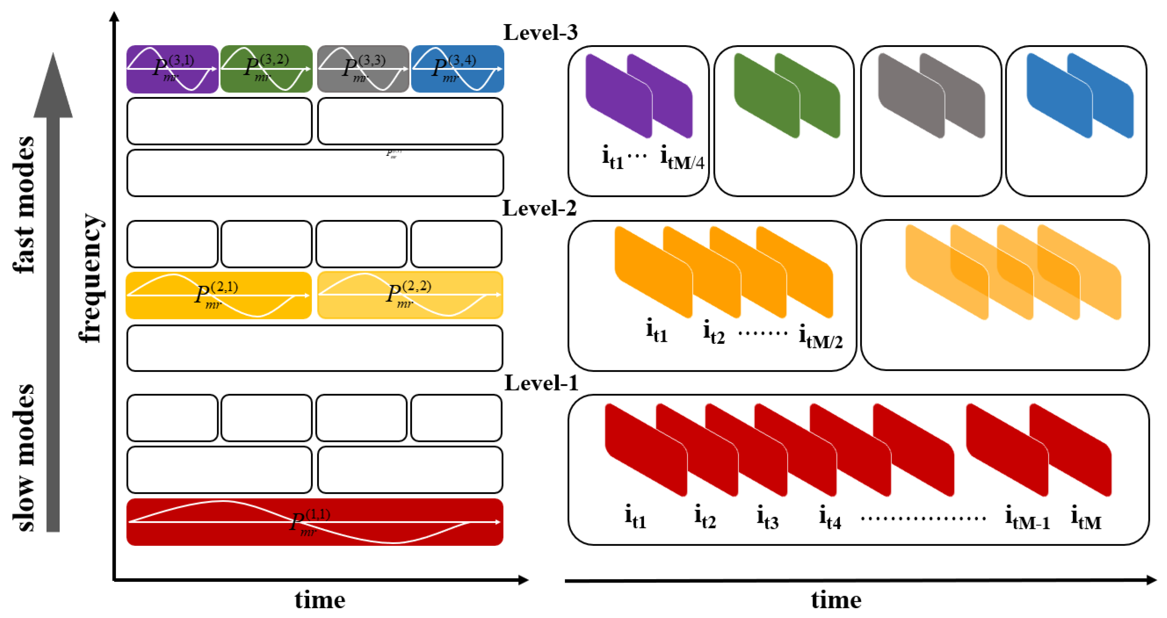Figure 8 offers a graphic portrayal elucidating the concept of multiscale analysis intrinsic to mrDMD. As delineated, myriad distinct compartments are delineated contingent upon both frequency and position within a specific temporal sequence. Each compartment bears the appellation $P_{mr}^{(b,c)}$ with b signifying the tier and c denoting the specific position within that tier.

In pursuit of mitigating discrepancies, wmrDMD adeptly orchestrates the adaptive fusion of individual reconstructions. This intricate process involves the intricate segmentation of matrix $n\times M\cdot N$, which encapsulates the comprehensive pressure dataset of the temporal continuum, into a multitude of matrices marked by their interwoven segments. The overarching principle underpinning the windowing methodology is the meticulous subdivision of the temporal sequence into a plethora of intersecting partitions. On each of these segments, a rigorous mrDMD analysis is meticulously executed. Subsequently, the composite amalgamation of all these overlapping reconstructions is artfully engineered, a task facilitated by the judicious application of weighting factors.

The temporal sequence of the dataset is delineated as an assemblage of manifold vectors, wherein $\ell$ represents an assortment of $p_i$ vectors, and n encapsulates the complete tally of frames within the chronological progression.

$$\ell =[p_0,p_1,\dots ,p_n]$$

(8)

Within the conventional milieu of mrDMD scrutiny, this temporal succession denominated as $\ell$ is harnessed to engender a plurality of multifarious reconstructions across disparate echelons of ${\ell }_i$.

$$\begin{array}{l}{\ell }_0=[p_{0,0},p_{0,1},\dots ,p_{0,n}]\\ {\ell }_1=[p_{1,0},p_{1,1},\dots ,p_{1,n/2}],[p_{1,(n/2)+1},\dots ,p_{1,n}]\\ {\ell }_2=[p_{2,0},p_{2,1},\dots ,p_{2,n/4}],[p_{2,(n/4)+1},\dots ,p_{2,n/2}],\\ \dots [p_{2,(3n/4)+1},\dots ,p_{2,n}]\end{array}$$

(9)

Utilizing these reconstitutions, it is feasible to regenerate the primordial chronological succession:

$$\ell \approx {\displaystyle \sum _{q=0}^k{\ell }_q}$$

(10)

Nonetheless, given the intricacies inherent in multi-resolution analysis, the temporal progression, in addition to its ${\ell }_0$ division, undergoes a partitioning operation across all strata, necessitating the reintegration of these partitions within each corresponding stratum. This amalgamation is effectuated through discrete arrays denoted as ${\ell }_1$ and ${\ell }_2$. These discrete arrays demarcate the loci responsible for deviation from the native chronological sequence during the reconstitution procedure, particularly when the model is employed to enhance the temporal resolution of measurements. To mitigate the complications arising from such divergence, a data windowing technique is employed.

Employing the windowing stratagem as elucidated in reference [34], the original chronological sequence is discretely partitioned into an assemblage of diminutive, intersecting temporal sequences, signified as ${\ell }^q$.

$$\begin{array}{l}{\ell }^0=[p_0,p_1,\dots ,p_{j_0}],\\ {\ell }^1=[p_{j_1},p_1,\dots ,p_{j_1^{’}}],\dots \\ {\ell }^M=[p_{j_M},p_1,\dots ,p_n]\end{array}$$

(11)

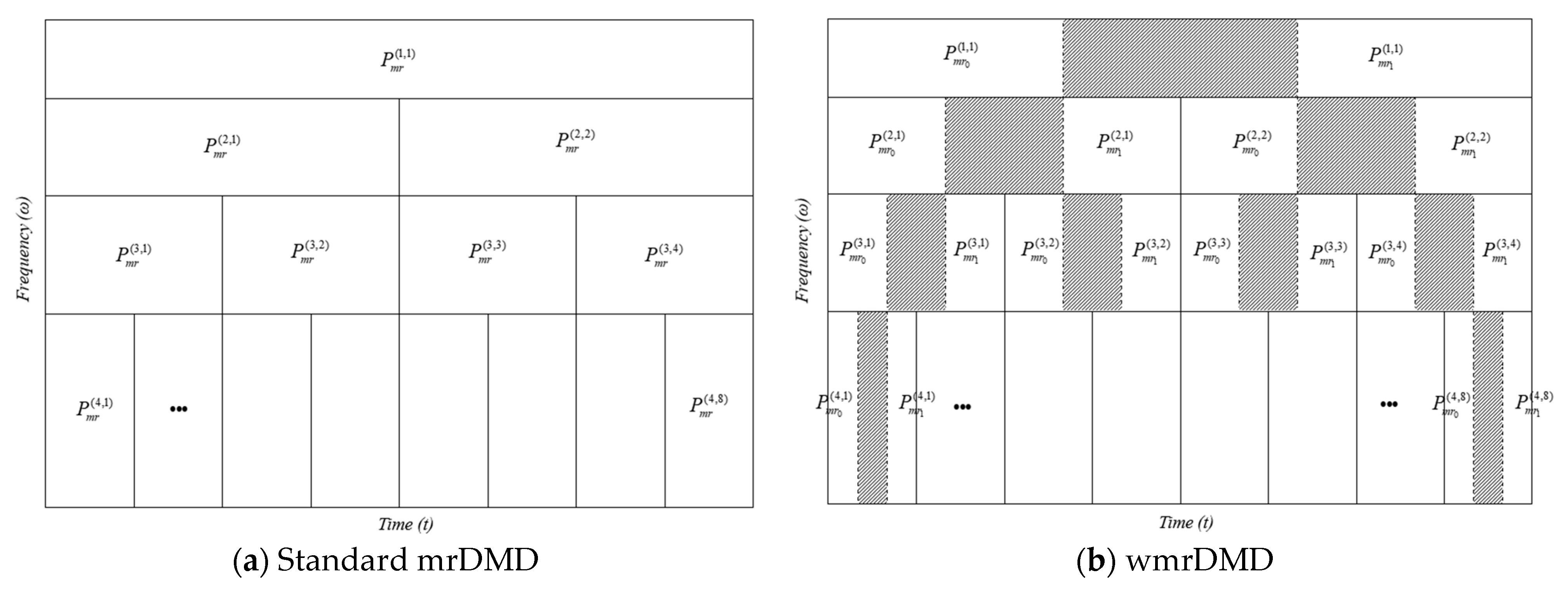
As shown in Figure 9, in this instance, the bifurcation of time series $j_0,j_1,j_1^{’},j_M,\dots$ is contingent upon both the aggregate frame count of the temporal sequence and the count of tiers integrated into the mrDMD algorithm, adhering to the correlation encapsulated in $j_0=j_1^{’}-j_1=n-j_M$. This stratagem is enacted to guarantee homogeneity across all time sequences ${\ell }^q$ situated within an equivalent tier, ensuring an identical frame tally and seamless overlap with concomitant temporal sequences bearing a congruous frame count. The comprehensive temporal sequence is an amalgamation encompassing the entirety of these interfusing time sequences:

$$\ell ={\displaystyle \underset{q=0}{\overset{M}{\cup }}{\ell }^q}$$

(12)

Subsequently, the mrDMD algorithm is administered to each and every temporal succession denoted as ${\ell }^i$. In this investigation, a 50% interlap ratio was chosen for contiguous temporal matrices, with each matrix encompassing two-thirds of the frames featured in the conventional mrDMD analysis. This procedure yields the ensuing matrices, which constitute the superimposed regenerations pertinent to each mrDMD echelon.

$$\begin{array}{l}{\ell }_0^1=[p_{0,1}^1,p_{0,2}^1,\dots ,p_{2n/3}^1],\\ {\ell }_0^2=[p_{0,(n/3)}^2,\dots ,p_n^3]\\ {\ell }_1^1=[p_{1,1}^1,p_{1,2}^1,\dots ,p_{3n/8}^1],[p_{1,n/8}^1,\dots ,p_{1,n/2}^1]\\ {\ell }_1^2=[p_{1,(n/2)+1}^2,\dots ,p_{1,7n/8}^2],[p_{1,5n/8}^2,\dots ,p_{1,n}^2]\end{array}$$

(13)

The application of the windowing stratagem does not abrogate the imperative of amalgamating the matrix into a solitary data manifestation; it does, however, successfully extirpate model disparities induced by this amalgamation, albeit introducing a staggered spatial configuration in the interstitial domains. This reconstructed staggered disposition serves as a palliative against the complications arising from dissimilitudes during the amalgamation process. The parameter governing the magnitude of this interstitial region, denominated as $P_{mr}(t)$, is demarcated by the modulating influence of the weighting coefficient, designated as ${\beta }_q$.

$$P_{mr}(t)={\beta }_i{\displaystyle \sum _{q=0}^k{\ell }_q^i}+{\beta }_{i+1}{\displaystyle \sum _{q=0}^k{\ell }_q^{i+1}}$$

(14)

$$\alpha =\max (1-\frac{\sqrt{{\displaystyle {\sum }_{t\in t_{match}}{\displaystyle {\sum }_S{(P(t,S)-P_{mr}(t,S))}^2}}}}{\sqrt{{\displaystyle {\sum }_{t\in t_{match}}{\displaystyle {\sum }_S{(P(t,S)+P_{mr}(t,S))}^2}}}},0)$$

(15)

$${\beta }_1=\frac{{\alpha }_1}{{\alpha }_1+{\alpha }_2},{\beta }_2=\frac{{\alpha }_2}{{\alpha }_1+{\alpha }_2},$$

(16)

Here, $t_{match}$ is delineated as the chronometric instances congruous with numerical simulation metrics and mrDMD regenerations. S signifies the quantified spatial constituent, or, in this instance, $P(t,S)$ signifies the aggregate of pixels within each frame. $P_{mr}(t,S)$ comprises the axial force information derived from the numerical simulation surveillance, and $\alpha$ comprises the pressure metrics obtained from mrDMD regenerations. The parameter e quantifies the degree of concordance between the regenerations and the data for a distinct array of frames.

In the realm of interpenetrating mrDMD restorations, amalgamation is achievable through the standardization of all remaining variables denoted as $\alpha$ within the coalescent temporal interval. This begets an illustrative instance of $\beta$, expounded upon in formula (16), wherein two regenerations interlace during a designated temporal span.

5. Calculation Results and Analysis

5.1. Model Validation

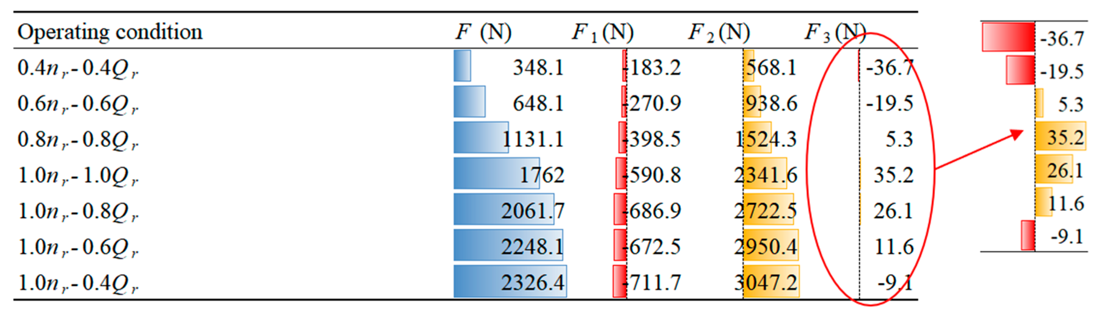
In accordance with the characteristics of a centrifugal pump, the total axial force (F) is comprised of the following components: the force exerted by the impeller front cover plate (F₁), the force exerted by the impeller back cover plate and shaft end (F₂), and the axial force generated by the impeller blades (F₃). Figure 10 depicts the direction of F₂.

The calculation formula for the total axial force F can be expressed as follows:

$$F=F_1+F_2+F_3$$

(17)

The original axial force data, comprising 180 data points for two complete cycles at three selected locations of axial force components under the design operating condition, are compared with the reconstructed axial force data obtained using wmrDMD and standard mrDMD, as depicted in Figure 10. Both wmrDMD and standard mrDMD show good agreement with the original axial force data, except for minor discrepancies typically observed at the extreme points of the curves, where the axial force displays the greatest variation. The performance of the wmrDMD algorithm at these points remains independent of the location and effectively improves the temporal resolution of the time series data.

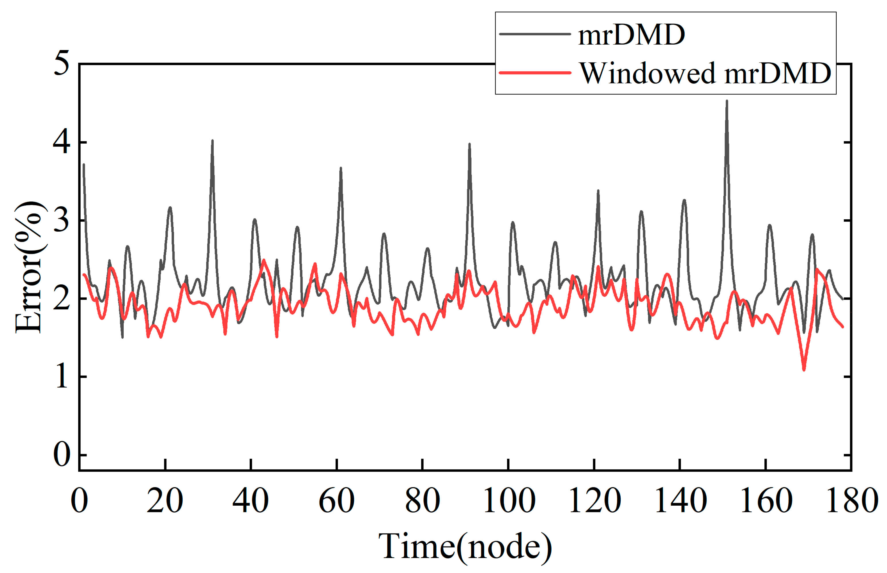
In order to assess the performance of the data-driven models generated by standard mrDMD and the validated models, the wmrDMD model under the design operating conditions is compared to the data-driven model of the centrifugal pump impeller’s axial force field created by standard mrDMD, along with the original axial force data of the impeller.

Figure 11 reveals that the reconstruction errors of the standard mrDMD range from 1.08% to 2.49%, whereas the reconstruction errors of wmrDMD range from 1.51% to 4.53%. It is worth noting that in Figure 11, standard mrDMD exhibits prominent errors primarily manifesting along the boundaries of each block. This occurs because the standard mrDMD introduces non-physical errors during the block partitioning process. In contrast, the wmrDMD algorithm effectively mitigates the non-physical errors between blocks. This indicates that applying the wmrDMD algorithm with the enhanced method can effectively alleviate the issue of divergence in comparison to the standard mrDMD, accurately modeling the time series data.

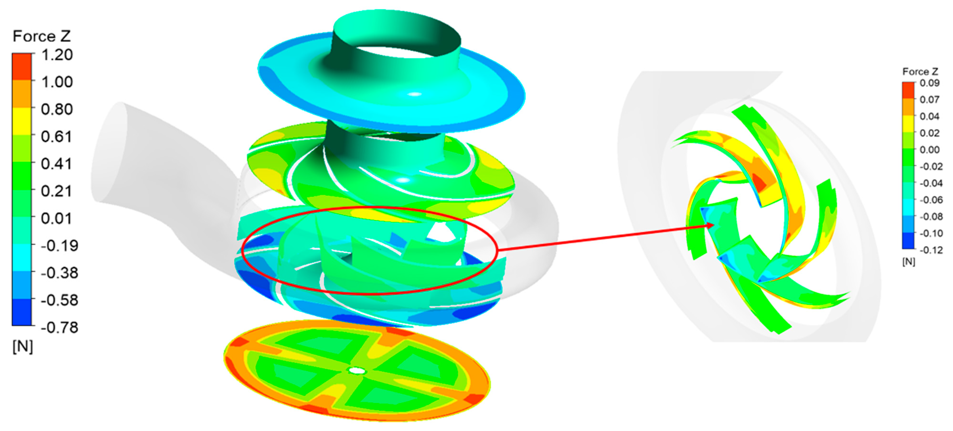
Based on Figure 12, it is possible to perform an analysis of the distribution of axial forces on the surfaces of the impeller, taking into account all surfaces subjected to axial forces under the design operating condition.

Figure 12 illustrates that the absolute values of axial forces on the outer surface of the impeller front cover plate exhibit an increasing trend with an expanding cross-sectional radius. The axial force values in the central region of the impeller exhibit a concentric circular distribution, being lower than those at the outer edge. Similarly, the distribution of axial forces on the inner surfaces of the impeller front and rear cover plates conforms to the same pattern. The axial force at the impeller inlet is the smallest, gradually increasing from the inner diameter to the outer diameter along the impeller flow passage. Near the impeller outlet, the maximum axial force is attained in proximity to the blade pressure surface. The outer surface of the impeller rear cover plate demonstrates axial symmetry, with the minimum axial force value located at the center of the outer surface within the 0–90° region (1/4 circle) of the impeller rear cover plate. Along the centerline, the axial force gradually increases from the inner diameter to the outer diameter. The axial forces on the blades are comparatively smaller than those on the impeller cover plates. The blade suction surface experiences the maximum downward axial force, likely attributed to the impact of the incoming water flow on the blades. The blade pressure surface undergoes the maximum upward axial force near the inlet, with the axial force gradually diminishing along the outlet due to the decreasing pressure gradient.

By conducting unsteady numerical simulations, the axial force (F) for three operating conditions, namely, 1.0n_r-1.0Q_r, 1.0n_r-0.8Q_r, 1.0n_r-0.6Q_r, 1.0n_r-0.4Q_r, and 0.8n_r-0.8Q_r, 0.6n_r-0.6Q_r, 0.4n_r-0.4Q_r, was determined and is presented in Figure 13.

By examining Figure 13, it is evident that as the flow rate decreases from 1.0Q_r to 0.4Q_r, both the axial force of the variable flow condition and its corresponding cover plate force increase. This indicates a continuous rise in pressure exerted on the impeller cover plates. The axial force is 1.31 times higher than the axial force under the design operating condition.

Conversely, during variable speed regulation, the axial force of the impeller and its corresponding cover plate force decrease, reflecting a continuous decrease in pressure applied to the impeller cover plates. The axial force is 19.74% of the axial force under the design operating condition.

Under variable operating conditions, the axial forces acting on the blades (F3) decrease. This finding aligns with the experimental results of Jin F. Y et al. [13], which demonstrated that the axial force (F3) acting on the blades transitions from positive to negative as the flow rate decreases. This suggests that the variation pattern of the axial force on the impeller cover plates differs from the axial force resulting from the pressure difference between the pressure surface and suction surface of the blades.

Based on the aforementioned analysis, it can be concluded that the forces on the impeller’s front and rear cover plates exert the greatest influence on the impeller’s axial force. Additionally, the axial force of the impeller demonstrates a linear variation pattern as the flow rate decreases. Therefore, the axial forces of the impeller under the 1.0n_r-1.0Q_r, 1.0n_r-0.4Q_r, and 0.4n_r-0.4Q_r operating conditions were selected for comparative analysis.

5.2. Multi-Resolution Analysis

To analyze the axial force field of the centrifugal pump impeller under the 1.0n_r-1.0Q_r, 1.0n_r-0.4Q_r, and 0.4n_r-0.4Q_r operating conditions, the wmrDMD method was employed. In order to balance computational accuracy and efficiency, a time step of 0.000229885 s was selected for the 1.0 speed condition, which corresponds to a time iteration of 4° per cycle. For the 0.4 speed condition, a time step of 0.000574712 s was utilized, also corresponding to a time iteration of 4° per cycle. In total, 540 time steps were analyzed, covering six cycles for each operating condition.

Figure 11 presents the wmrDMD multi-level plot of the blade axial force mode and its corresponding frequency under the 1.0n_r-1.0Q_r operating condition. The time–frequency domain was divided into classical pyramid diagrams, as depicted in the figure. Each level, from level 1 to level 5, has an upper limit resolution frequency.

$$f_s\times 2^{i-1}$$

(18)

f_s is the shaft frequency and i is the level number.

To facilitate a clear analysis of the transient variations in the axial force field of the impeller, the energy values of the axial force field were normalized by subtracting the average flow field. Furthermore, the frequency values were normalized by comparing them with the rotational frequency. In order to achieve a suitable level of time–frequency resolution, the number of levels was determined as $f_s\times 2^4$, with the current frequency at the terminal level truncated to 55. The relevant time nodes were set at 48, which corresponds to 3 × 2⁴.

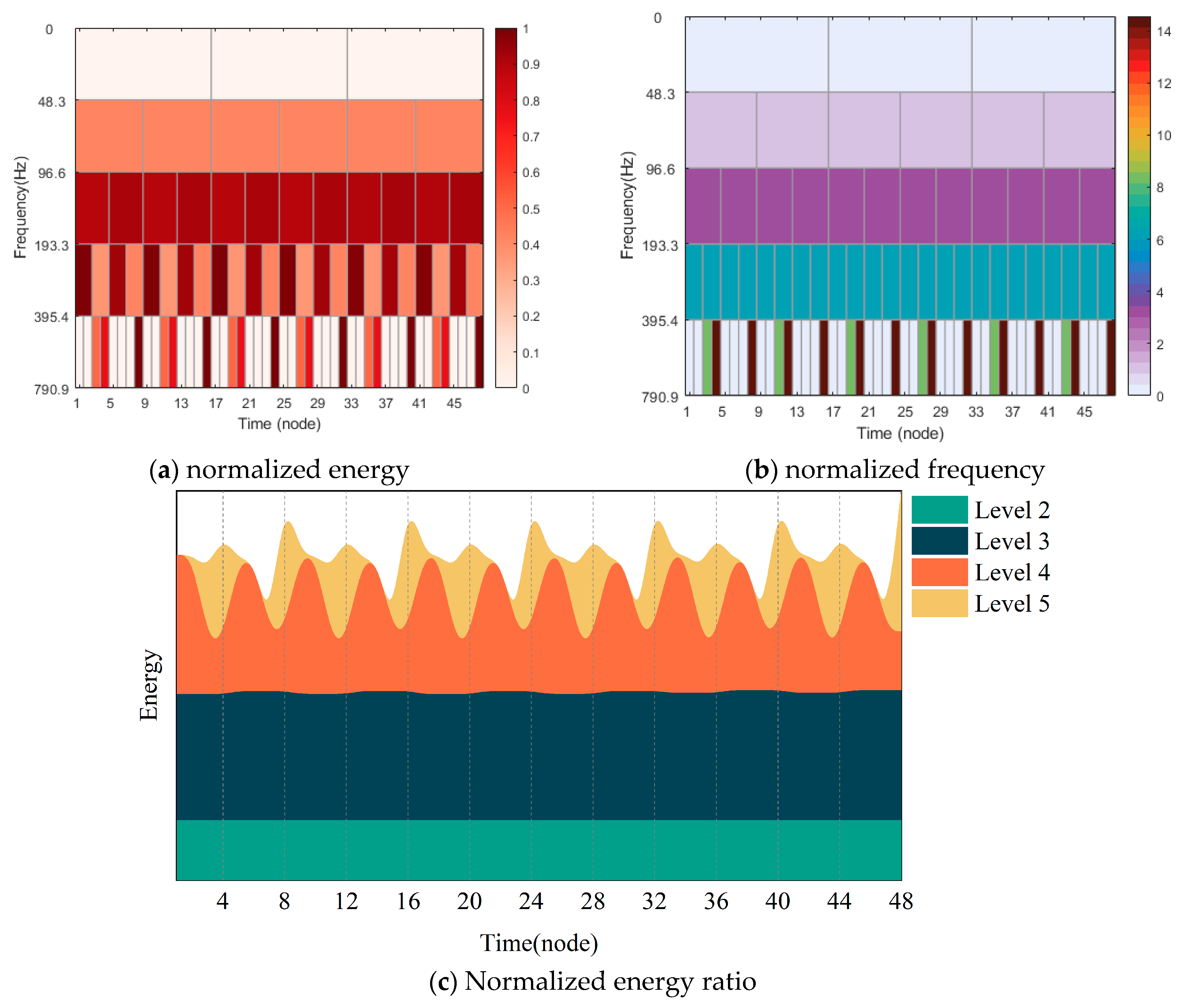
From Figure 14, it is evident that the fluctuation energy of the axial force of the impeller under the 1.0n_r-1.0Q_r operating condition was primarily concentrated in the third and fourth levels. The energy in the third level was the highest, corresponding to a frequency that was three times the shaft frequency. The energy in the fourth level was the second highest, corresponding to a frequency that was six times the shaft frequency. Both levels exhibited stable and periodic variations in energy, with frequencies that remained constant over time. Periodic oscillations of high-frequency energy were observed in the fifth level, alternating between presence and absence. This indicated the stability of the transformation in the axial force field under the 1.0n_r-1.0Q_r operating condition.

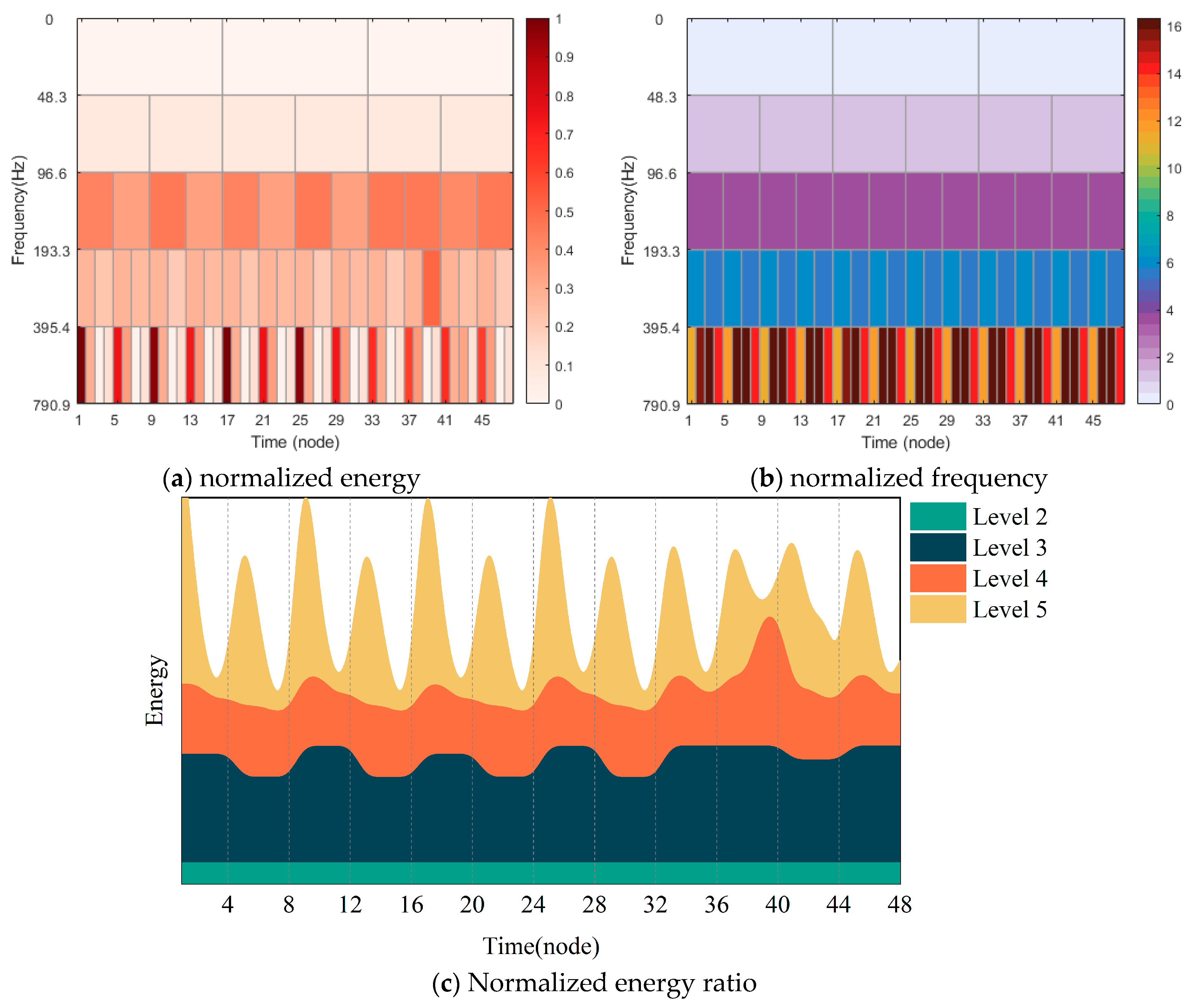
As seen in Figure 15, the 1.0n_r-0.4Q_r operating condition showed distinct characteristics. The axial force fluctuation energy in the third and fourth levels was relatively high and displayed minimal temporal variability, with frequencies ranging from 4 to 6 times the shaft frequency. Conversely, in the fifth level, the axial force fluctuation energy exhibited significant temporal fluctuations with a predominant frequency range of 11 to 16 times the shaft frequency. These temporal fluctuations were accompanied by noticeable transient features, indicating an unstable transformation of the axial force field in this specific operating condition.

In Figure 16, it is evident that the 0.4n_r-0.4Q_r operating condition demonstrated distinct characteristics. The axial force fluctuation energy in the third level of the impeller was notably high and exhibited minimal variability. The corresponding frequency was three times the shaft frequency. In the fourth level, the axial force fluctuation energy displayed significant temporal fluctuations, periodically alternating between four and six times the shaft frequency. Similarly, in the fifth level, the axial force fluctuation energy fluctuated over time, albeit with smaller variations, corresponding to nine and twelve times the shaft frequency. When compared to the 1.0n_r-1.0Q_r and 1.0n_r-0.4Q_r operating conditions, the energy and frequency variations were most stable under the 0.4n_r-0.4Q_r operating condition.

As shown in Figure 14, Figure 15 and Figure 16, it could be concluded that in all three operating conditions, the frequencies that influenced the axial force of the impeller exhibited stable periodic variations. In the 1.0n_r-1.0Q_r operating condition, a frequency of 14 times the shaft frequency was observed. In the 0.4n_r-0.4Q_r operating condition, a frequency of 12 times the shaft frequency was observed, while in the 1.0n_r-0.4Q_r operating condition, a frequency of 16 times the shaft frequency was observed. This indicated that the 1.0n_r-0.4Q_r operating condition resulted in more transient variations in the axial force field due to the presence of harmonics caused by the shaft frequency.

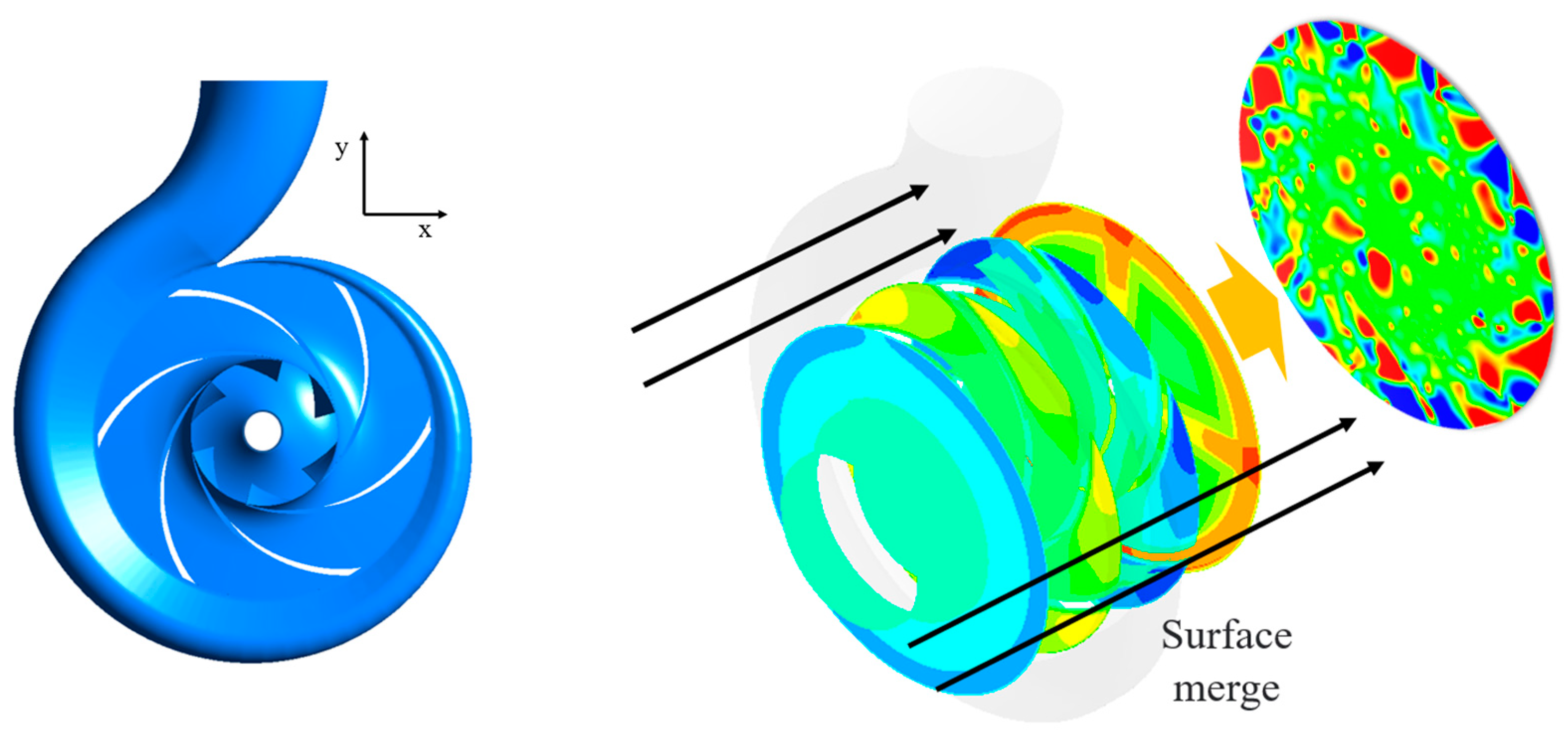
Figure 17 shows the relative positions of the centrifugal pump impeller and volute, along with their respective horizontal and vertical coordinates. This information is provided to facilitate the analysis of the oscillation positions of the impeller axial force. The axial force surface of the blade is combined. The utilization of the surface merging technique facilitates a clear observation of the overall force distribution on the surface.

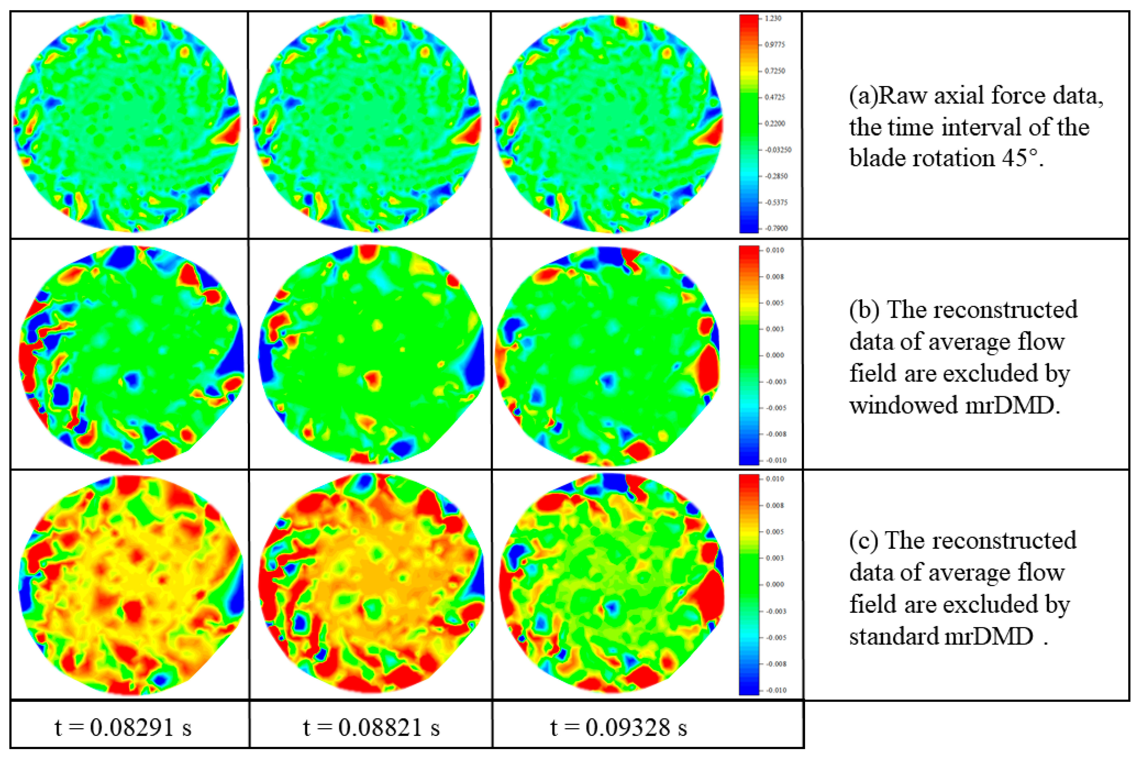
Figure 18a presents snapshots of the axial force field at intervals of 0.0053 s. As depicted in the figure, minimal differences can be observed in the axial force field over time due to the high energy of the mean flow field. The dominant energy of the mean flow field masks transient changes with higher frequencies but lower energy. Figure 18b illustrates the windowed mrDMD analysis, which isolates the mean flow field and captures high-frequency transient behavior. It is evident that the amplitude and position of the axial force vary over time. The energy of the high-frequency axial force is only approximately 1% of the energy of the mean flow field, making it challenging to observe these changes without isolating the mean flow field Figure 18c showcases the reconstructed axial force field data obtained using standard mrDMD. Similar to windowed mrDMD, standard mrDMD aims to capture transient behavior. However, due to non-physical influences during the reconstruction process, standard mrDMD is more difficult to isolate compared to windowed mrDMD. Standard mrDMD exhibits significant errors, particularly in regions with high pressure fluctuations, such as near oscillatory shock waves.

The final two cycles exhibiting the most substantial variations are selected and the wmrDMD characteristic modes of the axial force in the impeller at eight specific time points are observed. Each of these time points corresponds to 25% of a complete rotation cycle.

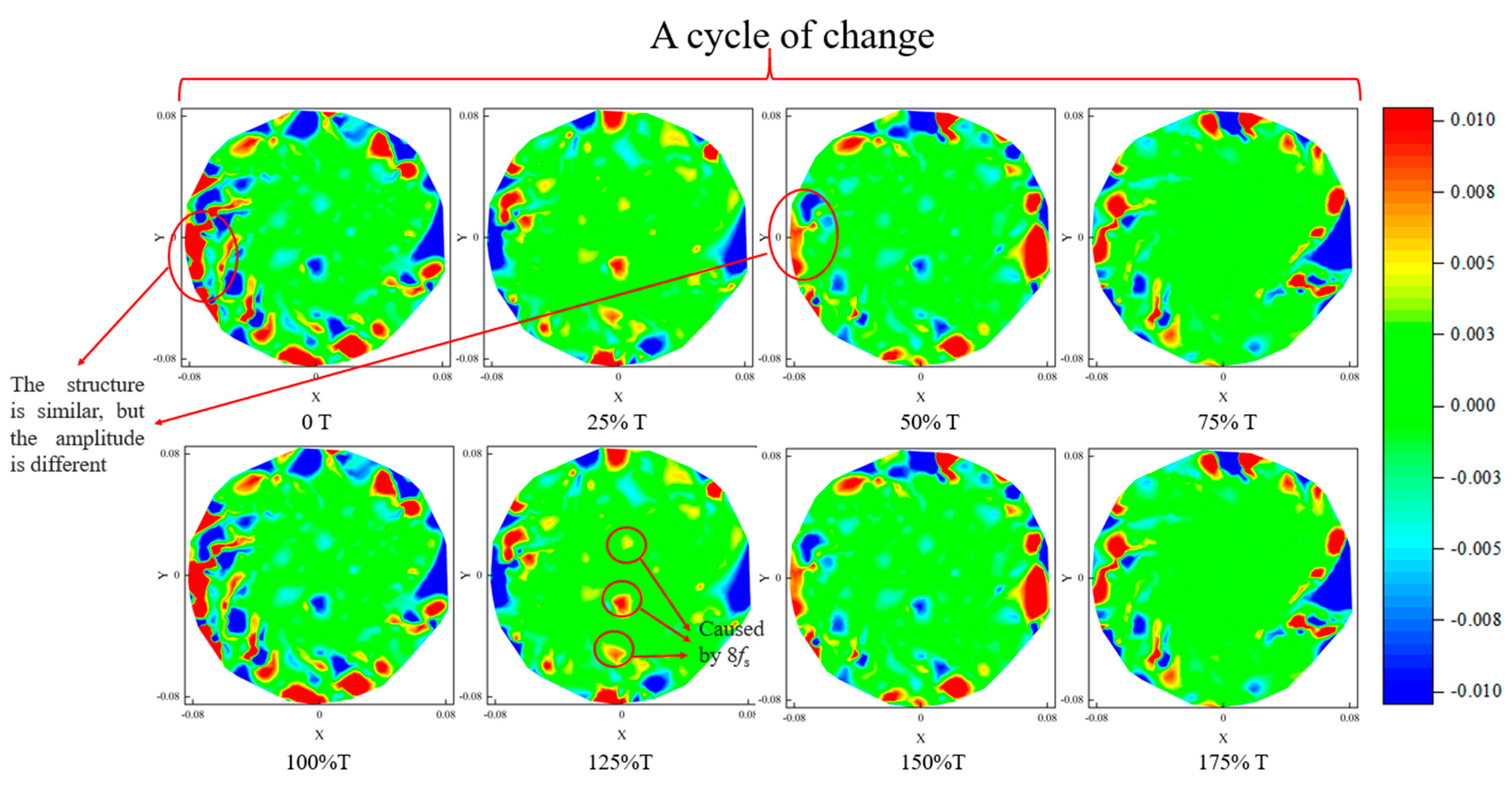
Figure 19 illustrates the characteristic modes of the axial force in the wmrDMD analysis for two rotation cycles under the operating condition of 1.0n_r-1.0Q_r. In the designed condition, the axial force variation precisely corresponds to one rotation cycle of the impeller. The dominant frequency influencing the axial force in Figure 19 was three times the shaft frequency. Transient behavior was primarily caused by frequencies at eight times and fourteen times the shaft frequency. The resulting oscillations in the axial force were concentrated mainly at the impeller outlet, and to a lesser extent at the impeller inlet. At the impeller inlet, the axial force predominantly exhibited positive values, which could be attributed to the asymmetrical structure of the centrifugal pump’s pump chambers. The dominant frequency driving variations during the transition from 0 T to 25% T (100% T to 125% T) was 8 f_s, with significant changes occurring at the impeller inlet. Moreover, during the transition from 0 T to 50% T (100% T to 150% T), the axial force structure maintained the same frequency but exhibited varying amplitudes. 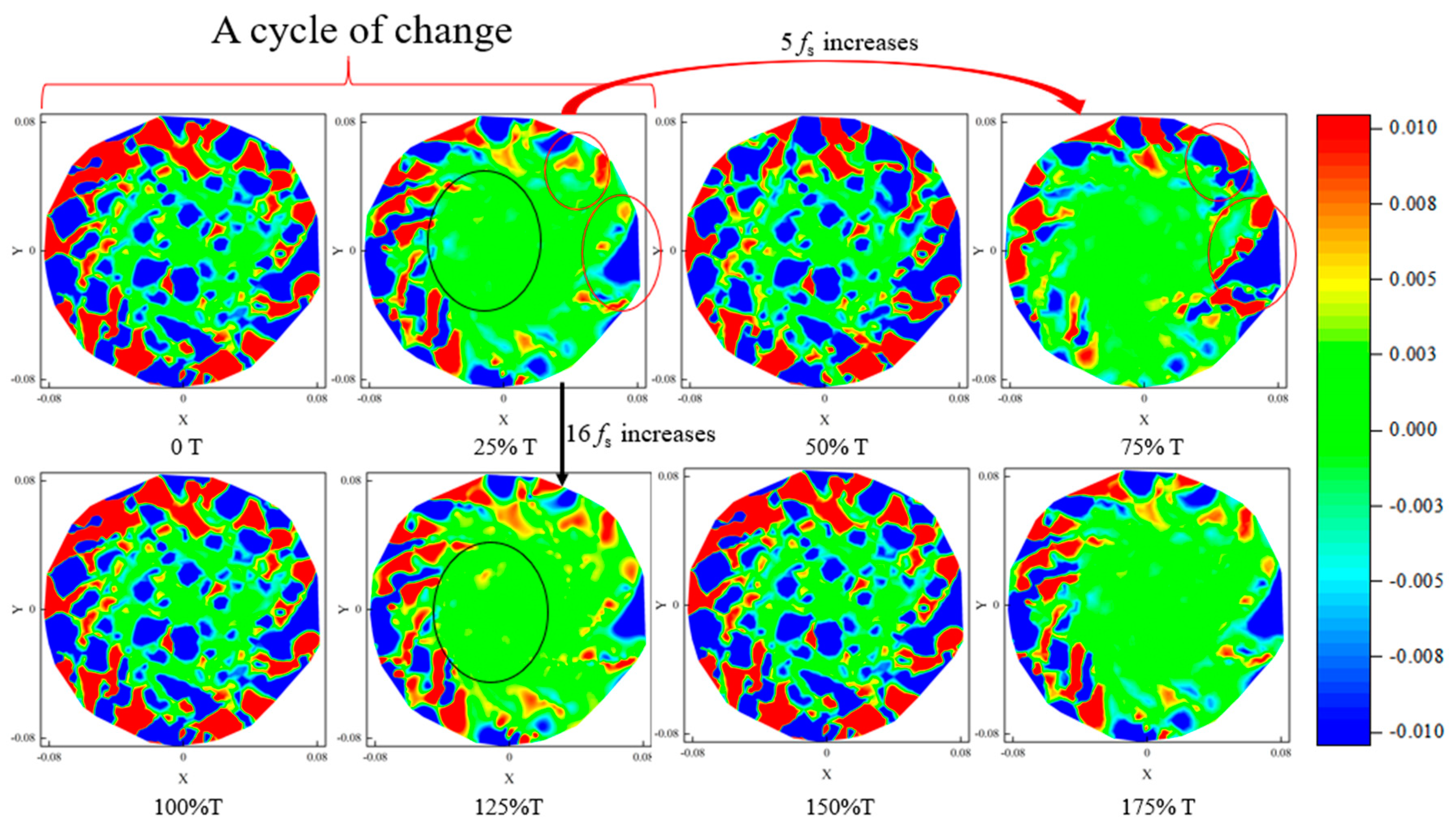Figure 20 presents the characteristic modes of axial force obtained from the wmrDMD analysis for two rotation cycles under the operating condition of 1.0n_r-0.4Q_r. It can be observed that, in the 1.0n_r-0.4Q_r condition, the axial force variation approximately corresponded to half a rotation cycle of the impeller. The dominant frequencies that influenced the axial force were primarily four times and six times the shaft frequency. Transient behavior primarily arose from frequencies ranging from eleven to sixteen times the shaft frequency. In comparison to the 1.0n_r-1.0Q_r operating condition, the 1.0n_r-0.4Q_r condition exhibited more significant axial force oscillations and structural changes, with the axial force distributed across the entire impeller. The axial force was highest at the impeller outlet and decreased towards the inlet. During the transition from 25% T to 75% T, the dominant frequency causing variations was 5 f_s, while during the transition from 25% T to 125% T, the dominant frequency was 16 f_s, with the most substantial axial force changes occurring at the inlet.

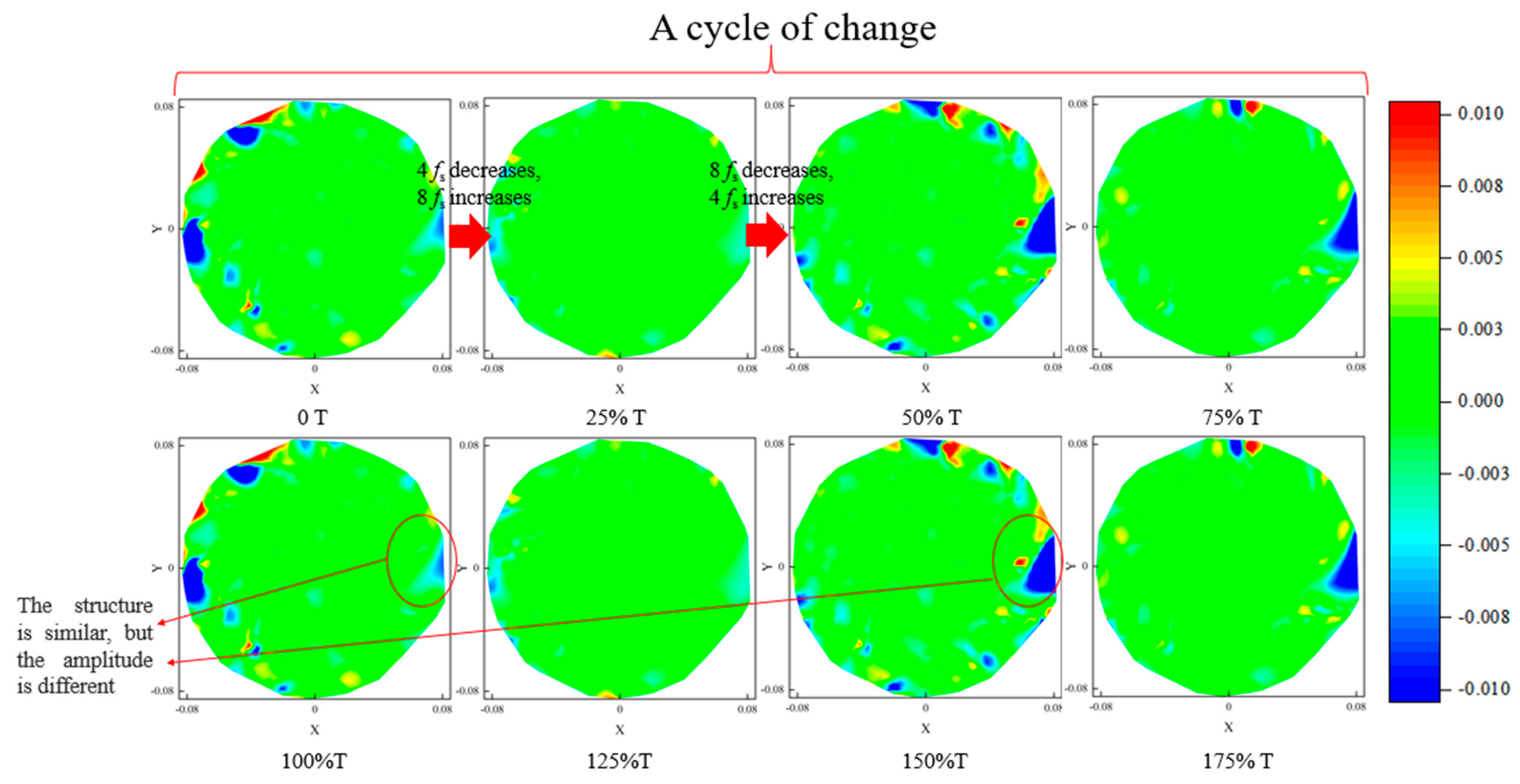
Figure 21 presents the characteristic modes of the axial force obtained from the wmrDMD analysis for two rotation cycles under the operating condition of 0.4n_r-0.4Q_r. In the 0.4n_r-0.4Q_r condition, the axial force variation precisely corresponded to one rotation cycle of the impeller. The axial force was primarily dominated by the frequency three times the shaft frequency. Transient behavior mainly arose from frequencies of four, six, nine, and twelve times the shaft frequency. Compared to the operating conditions of 1.0n_r-1.0Q_r and 1.0n_r-0.4Q_r, the 0.4n_r-0.4Q_r condition exhibited smaller axial force amplitudes and variations. The axial force was mainly concentrated at the outlet and was less pronounced at the inlet. During the transition from 0 T to 25% T (100% T to 125% T), the axial force increased due to the influence of eight times the shaft frequency, while it decreased due to the influence of four times the shaft frequency. The opposite trend was observed during the transition from 25% T to 50% T. The magnitude and variations of the axial force under the 0.4n_r-0.4Q_r condition indicated the most stable axial force oscillations of the impeller.

5.3. Cross-Wavelet and Wavelet Coherence Analysis

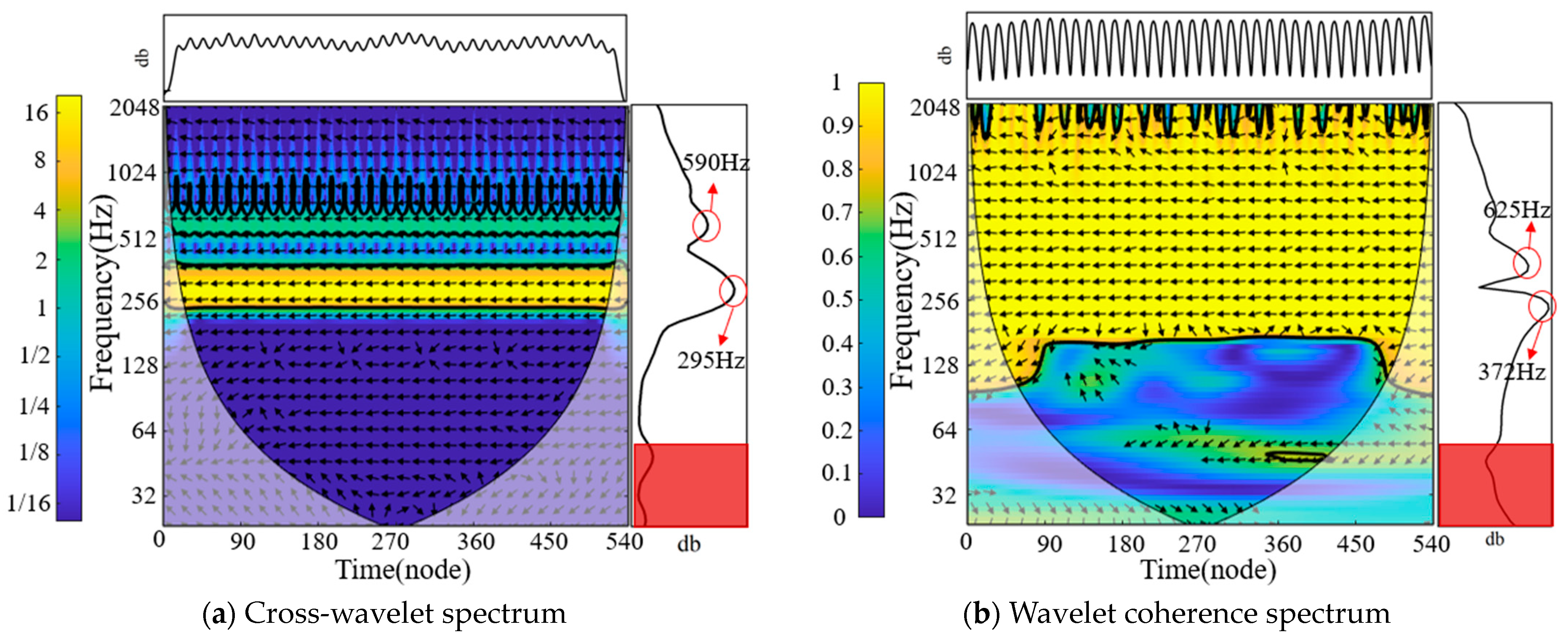
Cross-wavelet transform and wavelet coherence analysis are useful tools for examining the correlation, delay, and phase structure between different signals. In the context of this study, these analyses focused on the relationship between the axial forces on the front and back cover plates within the high-energy region of the time-frequency domain. The figure provides visual representations of these analyses.

In the figure below, the thick solid black line represents the region where the power spectrum passes the 95% red noise significance test. The solid thin line represents the cone of influence, indicating the boundary beyond which the power spectrum is affected by boundary effects and not considered. The arrows indicating phase differences between the two time series allow for the assessment of time lag correlation at different scale components. Right-pointing arrows indicate an in-phase relationship, while left-pointing arrows indicate an out-of-phase relationship.

Based on the significance of the axial forces on the front and back cover plates, as indicated in the table, it was evident that they had a substantial impact on the total axial force. Therefore, cross-wavelet and wavelet coherence analyses were conducted on the axial forces of the front and back cover plates for the 1.0n_r-1.0Q_r, 1.0n_r-0.4Q_r, and 0.4n_r-0.4Q_r operating conditions.

The cross-wavelet spectrum in Figure 22 reveals that the most significant power resonance periods for the axial forces on the front cover plate and rear cover plate were 256 Hz and 590 Hz, respectively. The wavelet coherence spectrum shows that 372 Hz and 625 Hz were strong common periodicities associated with the axial forces on the front cover plate and rear cover plate, exhibiting a negative correlation. Combining Figure 21, a strong correlation between the axial forces on the front cover plate and rear cover plate is observed in the frequency range of 372 Hz to 590 Hz.

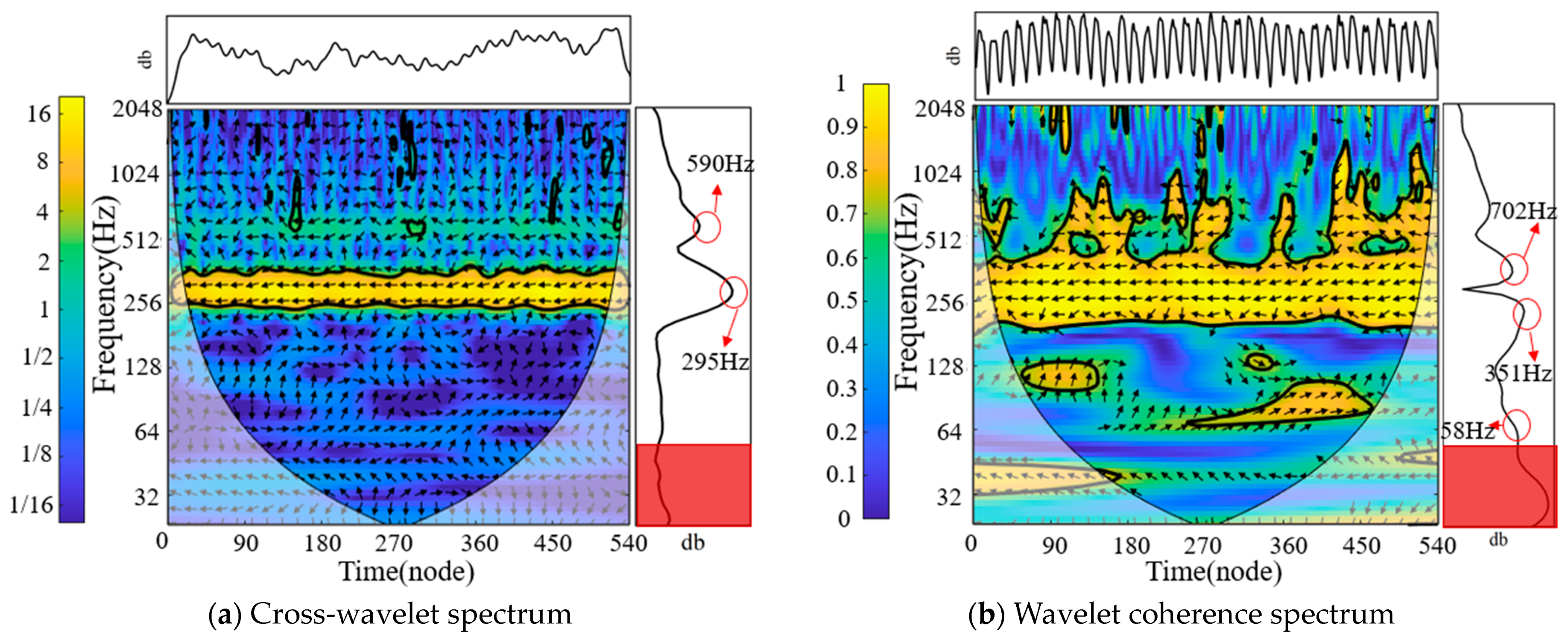
As seen in the cross-wavelet spectrum in Figure 23, the axial forces on the front cover plate and rear cover plate exhibited distinct power resonance periods at 256 Hz and 590 Hz, respectively. These resonances demonstrated a negative correlation, similar to the wavelet coherence spectrum observed in the design condition. However, the phase resonance periods appeared more chaotic, and the frequencies associated with higher power exhibited significant variations. The wavelet coherence spectrum revealed that the most significant common periodicity between the axial forces on the front cover plate and rear cover plate was 351 Hz, displaying a negative correlation. Notably, significant correlations were observed at 702 Hz and 58 Hz within specific time intervals, while the frequency range of 64 Hz to 128 Hz primarily exhibited positive correlation resonance periods, and the range of 420 Hz to 1024 Hz predominantly displayed negative correlation resonance periods. Combining the information from Figure 22a,b, a strong correlation between the axial forces on the front cover plate and rear cover plate is evident within the frequency range of 351 Hz to 590 Hz.

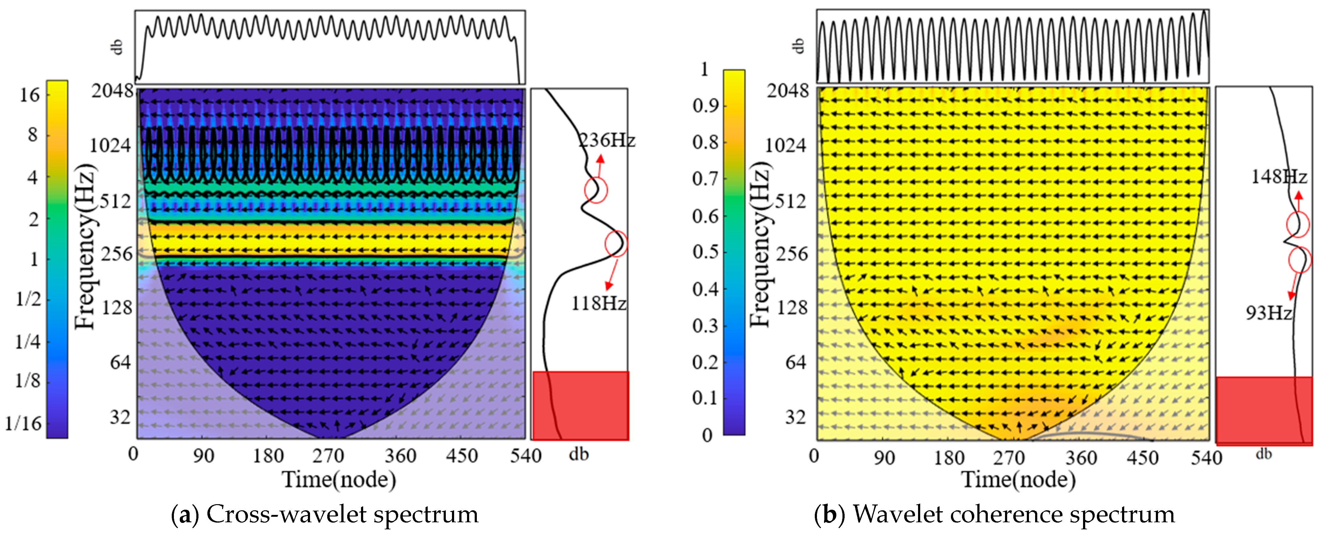
As seen in the cross-wavelet spectrum presented in Figure 24. it was evident that the axial forces on the front cover plate and rear cover plate exhibited significant power resonance periods at 118 Hz and 236 Hz, respectively. The wavelet coherence spectrum demonstrated a strong and consistent periodic relationship between these forces across nearly all frequencies, with the highest correlation observed at 93 Hz, followed by 148 Hz, both showing a negative correlation. By combining the information from Figure 23a,b, a clear correlation between the axial forces on the front cover plate and rear cover plate becomes apparent within the frequency range of 118 Hz to 148 Hz.

In the three aforementioned operating conditions, the power resonance periods of the front and rear cover plates exhibited no significant differences and were primarily concentrated within five to eight times the shaft frequency. However, notable discrepancies existed in their shared periodicity. Under the 0.4n_r-0.4Q_r condition, a strong negative correlation was consistently observed across the entire frequency range. In the 1.0n_r-1.0Q_r condition, a strong correlation was evident at the high-frequency ranges of 372 Hz and 625 Hz. In the 1.0n_r-0.4Q_r condition, significant correlations were observed not only at the high frequencies of 351 Hz and 702 Hz but also at the low frequency of 52 Hz throughout the entire time resolution range.

6. Discussion

The innovative wmrDMD technique offers several advantages in analyzing high-frequency dynamic behavior and modeling the flow field. It allows for accurate prediction of overall system behavior and future flow field structures, resulting in significant computational resource savings. Additionally, the wmrDMD technique utilizes classical mechanics’ well-known dynamics caused by forces, further enhancing its effectiveness.

One of the key strengths of the wmrDMD technique is its versatility. While initially applied to analyze axial forces in centrifugal pump impellers, it can be employed to improve the temporal resolution of any signal. Furthermore, the technique demonstrates strong generalizability and can be extended to three-dimensional data points. This implies that it can be successfully applied to various data collected from computational fluid dynamics simulations, with minor adjustments to the unfolding procedure.

By leveraging the capabilities of the wmrDMD technique, researchers can gain valuable insights into the dynamic behavior of complex systems, leading to improved modeling and predictive capabilities while minimizing computational resources.

While wmrDMD can effectively enhance temporal resolution, the precision of wmrDMD is still constrained by the Nyquist criterion. If the measurement rate of axial force is less than twice the axial force oscillation frequency, it is not feasible to accurately capture that frequency using wmrDMD. Overcoming the limitations imposed by the Nyquist criterion requires further development by future researchers.

7. Conclusions

A novel technique called windowed multi-resolution dynamic mode decomposition (wmrDMD) has been developed by combining a windowing function with the standard multi-resolution dynamic mode decomposition (mrDMD) technique. When applied to the temporal resolution decomposition of axial forces in centrifugal pump impellers, it has been observed that the standard mrDMD algorithm without windowing can lead to discrepancies in signal reconstruction. To address this, the enhanced wmrDMD technique was introduced, which reduces the discrepancies between the mrDMD model and the original data.

To evaluate the performance of the wmrDMD model, a comparison was conducted between the data-driven model and the original axial force field of the centrifugal pump impeller. The results showed that the error of the wmrDMD model was less than 2.49% for all pixels and time points, indicating its high accuracy in reconstructing the axial force field.

Using wavelet analysis and the wmrDMD technique, the axial forces of the centrifugal pump impeller were analyzed under three different operating conditions: 1.0n_r-1.0Q_r, 1.0n_r-0.4Q_r, and 0.4n_r-0.4Q_r. The findings revealed distinct characteristics in the behavior of the high-frequency axial forces. In the 1.0n_r-1.0Q_r condition, the axial forces exhibited stable periodic variations. In the 0.4n_r-0.4Q_r condition, the axial force demonstrated a consistently stable periodic fluctuation, albeit with negligible magnitude. However, in the 1.0n_r-0.4Q_r condition, the axial forces exhibited significant variations in both position and intensity without a stable trend.

Furthermore, the cross-wavelet and wavelet coherence analyses revealed that the axial forces of the impeller are primarily influenced by the axial forces on the front and back cover plates. The power resonance periods of the front and back cover plates were found to be concentrated around five to eight times the rotational frequency, with no significant differences between them. However, the periods of their joint variations showed notable distinctions. The 0.4n_r-0.4Q_r condition exhibited the strongest correlation, followed by the 1.0n_r-1.0Q_r condition, while the 1.0n_r-0.4Q_r condition showed the weakest correlation.