A Composite Framework Model for Transient Pressure Dynamics in Tight Gas Reservoirs Incorporating Stress Sensitivity

Abstract

Natural gas is an eco-friendly energy source with low carbon emissions, making it attractive globally. Understanding gas reservoirs is crucial for sustainable extraction and optimizing potential. However, the complicated fluid flow and production dynamics within intricate gas reservoirs, particularly those characterized by abnormally high pressures and tight porous media, remain partially understood and demand further investigation. In a tight porous medium subjected to high pressure, the assumption of constant permeability is no longer valid. Consequently, a novel composite seepage model has been developed in this study, which considers the responsiveness of permeability to stress. Perturbation theory is employed to address the inherent non-linearity demonstrated by the permeability modulus. The solution of dimensionless pressure responses under constant production conditions is accomplished in the Laplace domain by implementing integral transformation methods. Overall, a comprehensive model is provided to understand the production behaviors of tight gas reservoirs. Moreover, in order to comprehend the transient flow characteristics of tight gas reservoirs, log–log plots are generated through the Stehfest numerical inversion approach, with the flow regimes categorized based on the normalized time phases of the pressure curves. Parametric investigations reveal that stress sensitivity detrimentally affects permeability, resulting in more pronounced pressure declines during the intermediate and late flow phases. The transient seepage model elaborated in this study is able to consider the pertinent formation and well parameters. These interpreted parameters bear significance in designing hydraulic fracturing operations, assessing the potential of tight gas reservoirs, and ultimately enhancing gas production. The presented model not only enhances our understanding of the behavior of horizontal wells in stress-sensitive tight gas reservoirs but also makes a valuable contribution to the broader discussion on transient flow phenomena in petroleum engineering.

1. Introduction

Natural gas, distinguished by its convenience, stability, and high efficiency, constitutes a significant component of primary energy sources [1]. Despite its classification as a conventional fossil fuel, the carbon emissions stemming from its combustion are notably lower in comparison to coal and oil. Consequently, positioned as a comparatively cleaner fossil energy source, natural gas assumes a pivotal role within the landscape of energy transition processes. In recent years, there has been vigorous momentum in the exploration and development of natural gas, encompassing various forms such as conventional natural gas, coalbed methane, and shale gas [2,3]. The natural gas industry is committed to optimizing energy production and supply by harnessing various natural gas reservoirs. Of course, each natural gas reservoir possesses unique geological characteristics and production complexities. However, the complexity of fluid flow dynamics and production mechanisms in gas reservoirs remains incompletely understood, especially in reservoirs characterized by elevated pressures and tight porous media. Despite advancements in reservoir engineering, certain behaviors in these reservoirs remain enigmatic and necessitate further investigation. In other words, the extraction process from gas reservoirs with abnormally high-pressure conditions and tight porous structures presents multifaceted challenges. Intensified pressure and limited pore spaces lead to intricate interactions between fluid phases and the porous matrix. Understanding this interplay is crucial for optimizing production strategies and minimizing adverse consequences from suboptimal exploitation techniques. The geological response of reservoir rocks to continuous gas extraction requires careful consideration. Dynamic changes from gas withdrawal induce elastic deformation within the reservoir rock. Coupled with rising effective stress in the rock matrix, this leads to irreversible modifications in the reservoir’s physical attributes. An example is permeability stress-sensitivity, causing irreversible reduction due to stress–deformation interplay. In essence, understanding gas reservoir behavior in high-pressure, tight, porous formations is academically imperative. Advancing this comprehension not only facilitates sustainable gas extraction but also supports the development of reservoir management strategies aligned with broader environmental and energy goals.

Numerous efforts have been made to investigate the stress-sensitivity mechanism via laboratory experiments or physical modeling [4,5,6,7,8,9]. For example, Wang et al. established the relationship between overburden pressure and effective stress considering the stress arching effect in the Sulige gas field and proved that the stress sensitivity of permeability greatly depends on stress arching ratio [10]. A stress sensitivity evaluation standard was proposed by Xiao et al., considering experimental data and rock micro-structural features. This was achieved through an analysis of the empirical and theoretical models regarding the relationships between permeability and effective stress [11]. By employing conventional core plug sample measurements from carbonate formations, a relationship between permeability, porosity, velocity, and effective horizontal stress for carbonate reservoirs was formulated by Hamid et al. [12]. This correlation was established by integrating data obtained from both field observations and core measurements. In addition, evaluating the productivity losses caused by stress-dependent permeability has been widely studied in the actual reservoir engineering. Raghavan and Chin used a rigorous mathematical model that couples geo-mechanical and fluid-flow aspects to correlate productivity reductions with time [13], so that the reduction in the productivity index is expressed as a function of operating variables such as overburden stress, mechanical properties, wellbore pressure, drainage area, etc. A new pseudo pressure was defined by Fang and Yang to assess the collective impacts of stress, fluid flow, and alterations in reservoir properties on well performance [14]. Unlike the conventional deliverability model, this model features coefficients that are pressure-dependent and vary over the course of production time. Moreover, Lian et al. established a fracture closure model to analyze the well test data for abnormal pressure reservoirs, of which the productivity curve has a turning point on it [15]. A new procedure for quantifying permeability stress-sensitivity was introduced by Dou et al. [16]. This entailed the application of the traditional straight-line analysis method. The determination of the permeability modulus and formation parameters was achieved through the utilization of corrected pseudo-parameters, guided by the principle of cut-and-trial. Nonetheless, the aforementioned studies predominantly concentrated on steady productivity or absolute open flow, omitting consideration of transient production rates.

In the context of transient pressure or rate analysis, a multitude of studies have been devoted to the investigation of stress-dependent permeability [17,18,19,20,21,22]. Addressing the nonlinearity inherent in the seepage differential equation often involves the utilization of Pedrosa’s linearization method and perturbation technique [23,24,25]. An approximate equation was proposed by Zeng and Zhao for the analysis of transient pressure behavior of a well situated within a reservoir featuring multiple permeability anomalies [26]. Furthermore, Xiao et al. developed a numerical well test model capable of precisely determining gas reservoir parameters, acidizing effectiveness, and the extent of reduction in gas deliverability, where the dependency of the latter is contingent upon the “permeability modulus” [27]. A method was presented by Qanbari et al. to analyze transient linear flow within reservoirs featuring stress-sensitive permeability. This method employs production data; however, it does not encompass a comprehensive characterization of pressure responses during all flowing periods, such as the pseudo-radial flow period [28]. Additionally, Cai et al. analyzed the capillary-driven flow in gas-saturated porous media based on fractal theory and modified the classical Lucas–Washburn equation [29,30]. Wang et al. proposed an approximate analytical model to investigate the pressure transient in the naturally fractured reservoirs by a zero-order perturbation technique [31]. Finally, two inner boundary conditions and three outer boundary conditions were applied, i.e., in total, six solutions in the Laplace space were presented. Moreover, Zhao et al. and Ding et al. proposed new well productivity models of tight gas reservoirs, respectively, using numerical simulation and experimental methods [5,32]. Wu et al. conducted a transient model for volume fracturing vertical well, simultaneously considering the low-velocity non-Darcy flow and stress sensitivity [33]. Xu et al. conducted an investigation into the pressure behavior of multi-stage fractured horizontal wells, considering stress sensitivity and dual permeability within fractured gas reservoirs [22]. Similarly, Chu et al. proposed a novel semi-analytical monitoring model for a multi-horizontal well system in large-scale underground natural gas storage [34]. In order to expand their investigative scope, the analysis of production dynamics exhibited by various types of gas wells was undertaken by Xu et al. [35].

Based on the analysis of the literature and the previous discussion, it is anticipated that a comprehensive delineation of all transient pressure response flow periods can be achieved. This study promotes the field by developing a semi-analytical model for horizontal wells within tight gas reservoirs, accounting for permeability stress-sensitivity. Furthermore, the effects of the relevant factors are investigated.

2. Mathematical Model

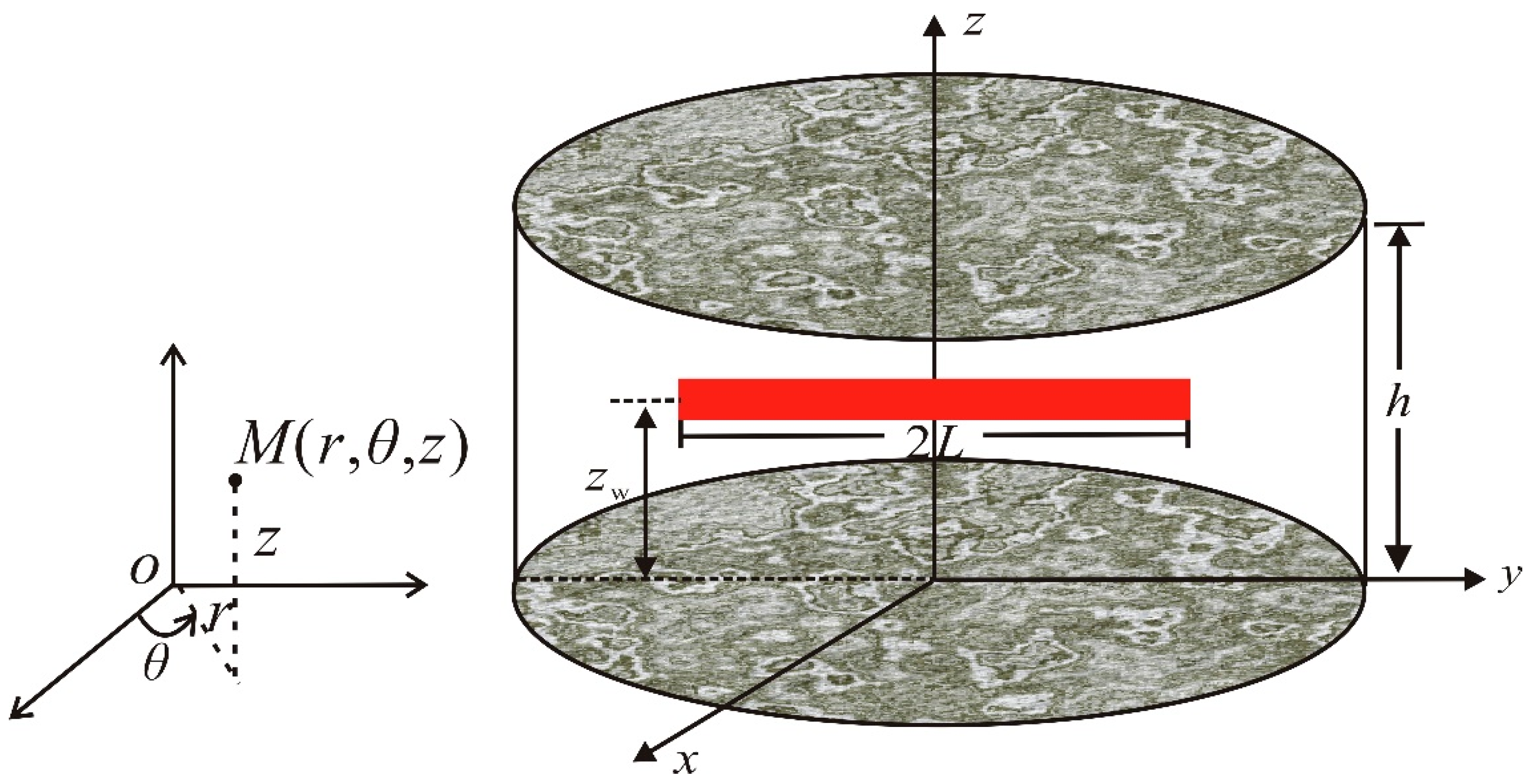
2.1. Description of Physical Model

If we consider alterations in reservoir permeability resulting from stress-sensitivity following the principles of the elastic rheological Hooke law, Pedrosa introduced the concept of the permeability modulus. This concept, akin to the compressibility coefficient, serves to characterize the correlation between changes in reservoir pressure and permeability. In the case of a single medium, its representation is given by

$$\gamma =\frac{1}{K}\frac{dK}{dp}$$

(1)

Typically, when the permeability modulus remains constant during the pressure reduction process, the subsequent integral of Equation (1) can be derived as follows:

$${\int }_K^{K_{\mathrm{i}}}\frac{1}{K}dK={\int }_p^{p_{\mathrm{i}}}\gamma dp$$

(2)

By solving Equation (2), we acquire

$$K=K_{\mathrm{i}}{e}^{-\gamma \left(p_{\mathrm{i}}-p\right)}$$

(3)

Likewise, following the concept of pseudo pressure, the definition of pseudo-permeability modulus is established as

$${\gamma }_{\mathrm{m}}=\frac{1}{\mathrm{K}}\frac{\mathrm{d}\mathrm{K}}{\mathrm{d}\mathrm{m}}$$

(4)

Upon integrating Equation (4), we derive

$$K=K_{\mathrm{i}}{e}^{-{\gamma }_{\mathrm{m}}\left(m_{\mathrm{i}}-m\right)}$$

(5)

where γ_m is the permeability modulus defined by pseudo pressure, mPa s/MPa²; m is pseudo pressure, MPa²/(mPa s).

Illustrated in Figure 1 is a physical depiction of a horizontal well in a tight gas reservoir, where a single-phase flow of natural gas is confined by two parallel impermeable planes at the upper and lower extents. Several assumptions are delineated as follows: The reservoir is regarded as a homogeneously porous medium characterized by an initial pressure of p_i, with its lateral boundary extending infinitely. The horizontal section, spanning a length of 2L, lies parallel to the enclosing upper and lower boundaries. Notably, the reservoir exhibits anisotropic properties, with horizontal and vertical permeabilities denoted as K_hi and K_vi, respectively, under the initial pressure. Stress sensitivity influences permeability. This influence is encapsulated by the permeability modulus, γ_m, which finds its definition in terms of pseudo pressure. The well operates by extracting gas at a consistent surface flow rate q_sc. The gas, exhibiting slight compressibility, maintains constant values for viscosity and the compressibility coefficient. Additionally, the ramifications of gravity and capillary forces are disregarded.

2.2. Governing Flow Equation of a Horizontal Well

By employing the mass balance equation and incorporating the state equation along with the motion equation, the governing flow equation for stress-sensitive behavior in a homogeneous tight medium can be formulated as

$$\frac{1}{r}\frac{\partial }{\partial r}\left[r{e}^{-{\gamma }_{\mathrm{m}}\left(m_{\mathrm{i}}-m\right)}\frac{\partial m}{\partial r}\right]+\frac{K_{\mathrm{vi}}}{K_{\mathrm{hi}}}\frac{\partial }{\partial z}\left[e^{-{\gamma }_{\mathrm{m}}\left(m_{\mathrm{i}}-m\right)}\frac{\partial m}{\partial z}\right]=\frac{\varnothing \mu C_{\mathrm{t}}}{3.6K_{\mathrm{hi}}}\frac{\partial m}{\partial t}$$

(6)

The initial expression on the left side of Equation (6) can be expressed as follows

$$\frac{1}{r}\frac{\partial }{\partial r}\left[r{e}^{-{\gamma }_{\mathrm{m}}\left(m_{\mathrm{i}}-m\right)}\frac{\partial m}{\partial r}\right]=e^{-{\gamma }_{\mathrm{m}}\left(m_{\mathrm{i}}-m\right)}\left[\frac{{\partial }^{2}m}{\partial r^2}+\frac{1}{r}\frac{\partial m}{\partial r}+{\gamma }_{\mathrm{m}}{\left(\frac{\partial m}{\partial r}\right)}^2\right]$$

(7)

Continuing with a similar methodology, the second term on the left side of Equation (6) transforms into

$$\frac{K_{\mathrm{vi}}}{K_{\mathrm{hi}}}\frac{\partial }{\partial z}\left[e^{-{\gamma }_{\mathrm{m}}\left(m_{\mathrm{i}}-m\right)}\frac{\partial m}{\partial z}\right]=\frac{K_{\mathrm{vi}}}{K_{\mathrm{hi}}}{e}^{-{\gamma }_{\mathrm{m}}\left(m_{\mathrm{i}}-m\right)}\left[\frac{{\partial }^{2}m}{\partial z^2}+{\gamma }_{\mathrm{m}}{\left(\frac{\partial m}{\partial z}\right)}^2\right]$$

(8)

By substituting (7) and (8) into Equation (6), we can obtain

$$\left[\frac{{\partial }^{2}m}{\partial r^2}+\frac{1}{r}\frac{\partial m}{\partial r}+{\gamma }_{\mathrm{m}}{\left(\frac{\partial m}{\partial r}\right)}^2\right]+\frac{K_{\mathrm{vi}}}{K_{\mathrm{hi}}}\left[\frac{{\partial }^{2}m}{\partial z^2}+{\gamma }_{\mathrm{m}}{\left(\frac{\partial m}{\partial z}\right)}^2\right]=e^{{\gamma }_{\mathrm{m}}\left(m_{\mathrm{i}}-m\right)}\frac{\varnothing \mu C_{\mathrm{t}}}{3.6K_{\mathrm{hi}}}\frac{\partial m}{\partial t}$$

(9)

Equation (9) represents the governing equation in pseudo pressure form for a horizontal well in tight gas reservoirs, accounting for the stress-dependent permeability.

2.3. Dimensionless Form of Seepage Model

Utilizing pertinent dimensionless definitions outlined in

Table 1. Definitions of the dimensionless variables.

Dimensionless pseudo pressure	$m_{\mathrm{D}}=\frac{78.489K_{\mathrm{hi}}h}{T{q}_{\mathrm{sc}}}\left(m_{\mathrm{i}}-m\right)$
Dimensionless pseudo permeability modulus	${\gamma }_{\mathrm{mD}}=\frac{T{q}_{\mathrm{sc}}}{78.489K_{\mathrm{hi}}h}{\gamma }_{\mathrm{m}}$
Dimensionless time	$t_{\mathrm{D}}=\frac{3.6K_{\mathrm{hi}}t}{\varnothing \mu C_{\mathrm{t}}{r}_{\mathrm{w}}^2}$
Dimensionless wellbore storage coefficient	$C_{\mathrm{D}}=\frac{0.159C}{\varnothing C_{\mathrm{t}}h{L}^2}$
Dimensionless horizontal section length	$L_{\mathrm{D}}=\frac{L}{h}\sqrt{\frac{K_{\mathrm{vi}}}{K_{\mathrm{hi}}}}$
Dimensionless gas reservoir thickness	$h_{\mathrm{D}}=\frac{h}{r_{\mathrm{w}}}\sqrt{\frac{K_{\mathrm{hi}}}{K_{\mathrm{vi}}}}$
Dimensionless radial distance	$r_{\mathrm{D}}=\frac{r}{L}$
Dimensionless wellbore radius	$r_{\mathrm{wD}}=\frac{r_{\mathrm{w}}}{L}$
Dimensionless vertical distance	$z_{\mathrm{D}}=\frac{z}{h}$
Dimensionless horizontal section position	$z_{\mathrm{wD}}=\frac{z_{\mathrm{w}}}{h}$

, the dimensionless flow differential equation, derived from Equation (9), can be derived as follows (i.e., (A12) in Appendix A):

$$\left[\frac{{\partial }^2{m}_{\mathrm{D}}}{\partial r_{\mathrm{D}}^2}+\frac{1}{r_{\mathrm{D}}}\frac{\partial m_{\mathrm{D}}}{\partial r_{\mathrm{D}}}-{\gamma }_{\mathrm{mD}}{\left(\frac{\partial m_{\mathrm{D}}}{\partial r_{\mathrm{D}}}\right)}^2\right]+L_{\mathrm{D}}^2\left[\frac{{\partial }^2{m}_{\mathrm{D}}}{\partial z_{\mathrm{D}}^2}-{\gamma }_{\mathrm{mD}}{\left(\frac{\partial m_{\mathrm{D}}}{\partial z_{\mathrm{D}}}\right)}^2\right]={\left(h_{\mathrm{D}}{L}_{\mathrm{D}}\right)}^2{e}^{{\gamma }_{\mathrm{mD}}{m}_{\mathrm{D}}}\frac{\partial m_{\mathrm{D}}}{\partial t_{\mathrm{D}}}$$

(10)

Initial condition:

$${\left.m_{\mathrm{D}}\right|}_{t_{\mathrm{D}}=0}=0$$

(11)

Inner boundary condition:

$$\underset{{\epsilon }_{\mathrm{D}}\to 0}{lim}\left[\underset{r_{\mathrm{D}}\to 0}{lim}{\int }_{z_{\mathrm{wD}}-\frac{{\epsilon }_{\mathrm{D}}}{2}}^{z_{\mathrm{wD}}+\frac{{\epsilon }_{\mathrm{D}}}{2}}\left(r_{\mathrm{D}}{e}^{{-\gamma }_{\mathrm{mD}}{m}_{\mathrm{D}}}\frac{\partial m_{\mathrm{D}}}{\partial r_{\mathrm{D}}}\right)d{z}_{\mathrm{wD}}\right]=-\frac{1}{2},\left|z_{\mathrm{D}}-z_{\mathrm{wD}}\right|\le \frac{{\epsilon }_{\mathrm{D}}}{2}$$

(12)

Infinite lateral boundary condition:

$${\left.m_{\mathrm{D}}\right|}_{r_{\mathrm{D}}\to \infty }=0$$

(13)

Enclosed top and bottom boundaries:

$${\left.\frac{\partial m_{\mathrm{D}}}{\partial z_{\mathrm{D}}}\right|}_{z_{\mathrm{D}}=0}=0, {\left.\frac{\partial m_{\mathrm{D}}}{\partial z_{\mathrm{D}}}\right|}_{z_{\mathrm{D}}=1}=0$$

(14)

Equations (10)–(14) constitute the mathematical framework governing a horizontal well in tight gas reservoirs.

2.4. Solution to Mathematical Model

When accounting for the influence of stress-sensitivity, it becomes evident that the seepage differential Equation (10) showcases a substantial level of nonlinearity, making direct solutions unfeasible. To address this, we employed the Pedrosa variable substitution and the regular perturbation method to mitigate the inherent nonlinearity. Subsequently, through the implementation of Laplace transformation (for the time variable) and orthogonal transformation (for the spatial variable) on the linearized model, the complex seepage differential equation can be transformed into a simpler Bessel equation. These transformations ultimately facilitate the achievement of accurate solutions.

2.4.1. Pedrosa Variable Substitution and Regularized Perturbation Method

As introduced by Pedrosa Jr. (1986) [23], the Pedrosa variable substitution takes the form of the following formula:

$$m_{\mathrm{D}}\left(r_{\mathrm{D}},z_{\mathrm{D}},t_{\mathrm{D}}\right)=-\frac{1}{{\gamma }_{\mathrm{mD}}}\mathit{ln}\left[1-{\gamma }_{\mathrm{mD}}{\xi }_{\mathrm{D}}\left(r_{\mathrm{D}},z_{\mathrm{D}},t_{\mathrm{D}}\right)\right]$$

(15)

where ${\xi }_{\mathrm{D}}\left(r_{\mathrm{D}},z_{\mathrm{D}},t_{\mathrm{D}}\right)$ is an intermediate variable, which is also called the perturbation deformation function.

By adhering to the rule of compound function derivation, we derived the subsequent formulas from Equation (15):

$$\left\{\begin{array}{l}{e}^{-m_{\mathrm{D}}{\gamma }_{\mathrm{mD}}}=1-{\gamma }_{\mathrm{mD}}{\xi }_{\mathrm{D}}\\ \frac{\partial m_{\mathrm{D}}}{\partial r_{\mathrm{D}}}=\frac{1}{1-{\gamma }_{\mathrm{mD}}{\xi }_{\mathrm{D}}}\frac{\partial {\xi }_{\mathrm{D}}}{\partial r_{\mathrm{D}}}\\ \frac{{\partial }^2{m}_{\mathrm{D}}}{\partial {r_{\mathrm{D}}}^2}=\frac{1}{1-{\gamma }_{\mathrm{mD}}{\xi }_{\mathrm{D}}}\frac{{\partial }^2{\xi }_{\mathrm{D}}}{\partial {r_{\mathrm{D}}}^2}+\frac{{\gamma }_{\mathrm{mD}}}{{\left(1-{\gamma }_{\mathrm{mD}}{\xi }_{\mathrm{D}}\right)}^2}{\left(\frac{\partial {\xi }_{\mathrm{D}}}{\partial r_{\mathrm{D}}}\right)}^2\\ \frac{\partial m_{\mathrm{D}}}{\partial z_{\mathrm{D}}}=\frac{1}{1-{\gamma }_{\mathrm{mD}}{\xi }_{\mathrm{D}}}\frac{\partial {\xi }_{\mathrm{D}}}{\partial z_{\mathrm{D}}}\\ \frac{{\partial }^2{m}_D}{\partial {z_{\mathrm{D}}}^2}=\frac{1}{1-{\gamma }_{\mathrm{mD}}{\xi }_{\mathrm{D}}}\frac{{\partial }^2{\xi }_{\mathrm{D}}}{\partial {z_{\mathrm{D}}}^2}+\frac{{\gamma }_{\mathrm{mD}}}{{\left(1-{\gamma }_{\mathrm{mD}}{\xi }_{\mathrm{D}}\right)}^2}{\left(\frac{\partial {\xi }_{\mathrm{D}}}{\partial z_{\mathrm{D}}}\right)}^2\\ \frac{\partial m_{\mathrm{D}}}{\partial t_{\mathrm{D}}}=\frac{1}{1-{\gamma }_{\mathrm{mD}}{\xi }_{\mathrm{D}}}\frac{\partial {\xi }_{\mathrm{D}}}{\partial t_{\mathrm{D}}}\end{array}\right.$$

(16)

By substituting (15) and (16) into the model described by Equations (10)–(14), the resultant expression is

$$\left\{\begin{array}{l}\frac{1}{r_{\mathrm{D}}}\frac{\partial }{\partial r_{\mathrm{D}}}\left(r_{\mathrm{D}}\frac{\partial {\xi }_{\mathrm{D}}}{\partial r_{\mathrm{D}}}\right)+L_{\mathrm{D}}^2\frac{{\partial }^2{\xi }_{\mathrm{D}}}{\partial {z_{\mathrm{D}}}^2}={\left(h_{\mathrm{D}}{L}_{\mathrm{D}}\right)}^2\frac{1}{1-{\gamma }_{\mathrm{mD}}{\xi }_{\mathrm{D}}}\frac{\partial {\xi }_{\mathrm{D}}}{\partial t_{\mathrm{D}}}\\ {\left.{\xi }_{\mathrm{D}}\right|}_{t_{\mathrm{D}}=0}=0\\ \underset{{\epsilon }_{\mathrm{D}}\to 0}{lim}\left[\underset{r_{\mathrm{D}}\to 0}{lim}{\int }_{z_{\mathrm{wD}}-\frac{{\epsilon }_{\mathrm{D}}}{2}}^{z_{\mathrm{wD}}+\frac{{\epsilon }_{\mathrm{D}}}{2}}\left(r_{\mathrm{D}}\frac{\partial {\xi }_{\mathrm{D}}}{\partial r_{\mathrm{D}}}\right)d{z}_{\mathrm{wD}}\right]=-\frac{1}{2},\left|z_{\mathrm{D}}-z_{\mathrm{wD}}\right|\le \frac{{\epsilon }_{\mathrm{D}}}{2}\\ {\left.{\xi }_{\mathrm{D}}\right|}_{r_{\mathrm{D}}\to \infty }=0\\ {\left.\frac{\partial {\xi }_{\mathrm{D}}}{\partial z_{\mathrm{D}}}\right|}_{z_{\mathrm{D}}=0}=0\hspace{0.33em},\hspace{0.33em}{\left.\frac{\partial {\xi }_{\mathrm{D}}}{\partial z_{\mathrm{D}}}\right|}_{z_{\mathrm{D}}=1}=0\end{array}\right.$$

(17)

Following the principles of regular perturbation theory, the terms ${\xi }_{\mathrm{D}}$, $\frac{1}{1-{\gamma }_{\mathrm{mD}}{\xi }_{\mathrm{D}}}$ and $-\frac{1}{{\gamma }_{\mathrm{mD}}}\mathit{ln}\left(1-{\gamma }_{\mathrm{mD}}{\xi }_{\mathrm{D}}\right)$ in (17) can be expressed as power series expansions in terms of the dimensionless permeability modulus, which take the form of

$${\xi }_{\mathrm{D}}={\xi }_{\mathrm{D}0}+{\gamma }_{\mathrm{mD}}{\xi }_{\mathrm{D}1}+{\gamma }_{\mathrm{mD}}^2{\xi }_{\mathrm{D}2}\cdots$$

(18)

$$\frac{1}{1-{\gamma }_{\mathrm{mD}}{\xi }_{\mathrm{D}}}=1+{\gamma }_{\mathrm{mD}}{\xi }_{\mathrm{D}}+{{\gamma }_{\mathrm{mD}}}^2{{\xi }_{\mathrm{D}}}^2\cdots$$

(19)

$$-\frac{1}{{\gamma }_{\mathrm{mD}}}\mathit{ln}\left(1-{\gamma }_{\mathrm{mD}}{\xi }_{\mathrm{D}}\right)={\xi }_{\mathrm{D}}+\frac{1}{2}{\gamma }_{\mathrm{mD}}{{\xi }_{\mathrm{D}}}^2+\cdots$$

(20)

Considering the typically small value of the dimensionless permeability modulus (${\gamma }_{\mathrm{mD}}<<1$), the zero-order approximation solution suffices to meet engineering accuracy standards. Consequently, the model (17) simplifies to

$$\left\{\begin{array}{l}\frac{1}{r_{\mathrm{D}}}\frac{\partial }{\partial r_{\mathrm{D}}}\left(r_{\mathrm{D}}\frac{\partial {\xi }_{\mathrm{D}0}}{\partial r_{\mathrm{D}}}\right)+L_{\mathrm{D}}^2\frac{{\partial }^2{\xi }_{\mathrm{D}0}}{\partial {z_{\mathrm{D}}}^2}={\left(h_{\mathrm{D}}{L}_{\mathrm{D}}\right)}^2\frac{\partial {\xi }_{\mathrm{D}0}}{\partial t_{\mathrm{D}}}\\ {\left.{\xi }_{\mathrm{D}0}\right|}_{t_{\mathrm{D}}=0}=0\\ \underset{{\epsilon }_{\mathrm{D}}\to 0}{lim}\left[\underset{r_{\mathrm{D}}\to 0}{lim}{\int }_{z_{\mathrm{wD}}-\frac{{\epsilon }_{\mathrm{D}}}{2}}^{z_{\mathrm{wD}}+\frac{{\epsilon }_{\mathrm{D}}}{2}}\left(r_{\mathrm{D}}\frac{\partial {\xi }_{\mathrm{D}0}}{\partial r_{\mathrm{D}}}\right)d{z}_{\mathrm{wD}}\right]=-\frac{1}{2},\left|z_{\mathrm{D}}-z_{\mathrm{wD}}\right|\le \frac{{\epsilon }_{\mathrm{D}}}{2}\\ {\left.{\xi }_{\mathrm{D}0}\right|}_{r_{\mathrm{D}}\to \infty }=0\\ {\left.\frac{\partial {\xi }_{\mathrm{D}0}}{\partial z_{\mathrm{D}0}}\right|}_{z_{\mathrm{D}}=0}=0\hspace{0.33em},\hspace{0.33em}{\left.\frac{\partial {\xi }_{\mathrm{D}0}}{\partial z_{\mathrm{D}0}}\right|}_{z_{\mathrm{D}}=1}=0\end{array}\right.$$

(21)

2.4.2. Laplace Transformation on Time Variable

The Laplace transform stands as a classical technique employed for solving partial differential equations, particularly those characterized by constant coefficients. This method entails a transformation of the time variable within the original function. By employing initial conditions to eliminate terms involving time derivatives, the result is an ordinary differential equation within the Laplace domain that corresponds to the spatial variables. Notably, the Laplace transform holds significant importance across the spectrum of oil and gas reservoir flow theory.

When subjected to the Laplace transformation, the mathematical Formulation (21) can be represented in the Laplace domain as follows:

$$\left\{\begin{array}{l}\frac{1}{r_{\mathrm{D}}}\frac{\partial }{\partial r_{\mathrm{D}}}\left(r_{\mathrm{D}}\frac{\partial {\overline{\xi }}_{\mathrm{D}0}}{\partial r_{\mathrm{D}}}\right)+L_{\mathrm{D}}^2\frac{{\partial }^2{\overline{\xi }}_{\mathrm{D}0}}{\partial {z_{\mathrm{D}}}^2}={\left(h_{\mathrm{D}}{L}_{\mathrm{D}}\right)}^{2}s{\overline{\xi }}_{\mathrm{D}0}\\ \underset{{\epsilon }_{\mathrm{D}}\to 0}{lim}\left[\underset{r_{\mathrm{D}}\to 0}{lim}{\int }_{z_{\mathrm{wD}}-\frac{{\epsilon }_{\mathrm{D}}}{2}}^{z_{\mathrm{wD}}+\frac{{\epsilon }_{\mathrm{D}}}{2}}\left(r_{\mathrm{D}}\frac{\partial {\xi }_{\mathrm{D}0}}{\partial r_{\mathrm{D}}}\right)d{z}_{\mathrm{wD}}\right]=-\frac{1}{2s},\left|z_{\mathrm{D}}-z_{\mathrm{wD}}\right|\le \frac{{\epsilon }_{\mathrm{D}}}{2}\\ {\left.{\xi }_{\mathrm{D}0}\right|}_{r_{\mathrm{D}}\to \infty }=0\\ {\left.\frac{\partial {\xi }_{\mathrm{D}0}}{\partial z_{\mathrm{D}0}}\right|}_{z_{\mathrm{D}}=0}=0\hspace{0.33em},\hspace{0.33em}{\left.\frac{\partial {\xi }_{\mathrm{D}0}}{\partial z_{\mathrm{D}0}}\right|}_{z_{\mathrm{D}}=1}=0\end{array}\right.$$

(22)

where s is the Laplace transformation variable.

2.4.3. Orthogonal Transformation on Spatial Variables

Before initiating the process of orthogonal transformation concerning the spatial variable $z_D$ within the model (22), it becomes imperative to address a Sturm–Liouville eigenvalue problem pertaining to $Z\left(z_D\right)$. This particular problem encapsulates a Sturm–Liouville equation and relevant boundary conditions. The objective of solving this eigenvalue problem is to determine the orthogonal transformation kernel, which essentially constitutes a set of complete orthogonal functions. In line with the principles of Sturm–Liouville eigenvalue theory, the resulting eigenfunctions manifest as $Z_n\left(z_D\right)=\mathit{cos}n\pi z_D$ (where n = 0, 1, 2...). These eigenfunctions, when combined with the weighted function $g\left(z_D\right)$, collectively establish an exhaustive orthogonal system spanning the domain [0, 1].

With this foundation, the subsequent step involves performing an orthogonal transformation on the spatial variable $Z\left(z_D\right)$. This process is articulated as follows:

$${\stackrel{=}{\xi }}_{\mathrm{D}0}={\int }_0^1{\overline{\xi }}_{\mathrm{D}0}\left(r_{\mathrm{D}},z_{\mathrm{D}}\right)\mathit{cos}n\pi z_{\mathrm{D}}d{z}_{\mathrm{D}}$$

(23)

The model (22) can undergo an orthogonal transformation, leading to the expression

$$\left\{\begin{array}{l}\frac{1}{r_{\mathrm{D}}}\frac{\partial }{\partial r_{\mathrm{D}}}\left(r_{\mathrm{D}}\frac{\partial {\stackrel{=}{\xi }}_{\mathrm{D}0}}{\partial r_{\mathrm{D}}}\right)-\left[{\left(h_{\mathrm{D}}{L}_{\mathrm{D}}\right)}^{2}s+n^2{\pi }^2{L}_{\mathrm{D}}^2\right]{\stackrel{=}{\xi }}_{\mathrm{D}0}=0\\ \underset{r_{\mathrm{D}}\to 0}{lim}{r}_{\mathrm{D}}\frac{\partial {\stackrel{=}{\xi }}_{\mathrm{D}0}}{\partial r_{\mathrm{D}}}=\frac{-\mathit{cos}n\pi z_{\mathrm{wD}}}{2s}\\ \\ {\left.{\stackrel{=}{\xi }}_{\mathrm{D}0}\right|}_{r_{\mathrm{D}}\to \infty }=0\end{array}\right.$$

(24)

By introducing the notation $u_{\mathrm{n}}={\left(h_{\mathrm{D}}{L}_{\mathrm{D}}\right)}^{2}s+n^2{\pi }^2{L}_{\mathrm{D}}^2$, the differential equation corresponding to model (24) can be restated as follows:

$$\frac{{\partial }^2{\stackrel{=}{\xi }}_{\mathrm{D}0}}{\partial r_{\mathrm{D}}^2}+\frac{1}{r_{\mathrm{D}}}\frac{\partial {\stackrel{=}{\xi }}_{\mathrm{D}0}}{\partial r_{\mathrm{D}}}-u_n{\stackrel{=}{\xi }}_{\mathrm{D}0}=0$$

(25)

Multiply both sides of Equation (25) by $r_{\mathrm{D}}^2$ to obtain

$$r_{\mathrm{D}}^2\frac{{\partial }^2{\stackrel{=}{\xi }}_{\mathrm{D}0}}{\partial r_{\mathrm{D}}^2}+r_{\mathrm{D}}\frac{\partial {\stackrel{=}{\xi }}_{\mathrm{D}0}}{\partial r_{\mathrm{D}}}-u_n{r}_{\mathrm{D}}^2{\stackrel{=}{\xi }}_{\mathrm{D}0}=0$$

(26)

Let us introduce a new variable, $x=r_{\mathrm{D}}\sqrt{u_n}$. Consequently, $r_{\mathrm{D}}$ can be expressed as $r_{\mathrm{D}}=\frac{x}{\sqrt{u_n}}$. Employing the rule of compound function derivation, Equation (26) can be converted to

$$r_{\mathrm{D}}^2{u}_n\frac{{\partial }^2{\stackrel{=}{\xi }}_{\mathrm{D}0}}{\partial x^2}+r_{\mathrm{D}}\sqrt{u_n}\frac{\partial {\stackrel{=}{\xi }}_{\mathrm{D}0}}{\partial x}-r_{\mathrm{D}}^2{u}_n{\stackrel{=}{\xi }}_{\mathrm{D}0}=0$$

(27)

This leads to the equation $x^2\frac{{\partial }^2{\stackrel{=}{\xi }}_{\mathrm{D}0}}{\partial x^2}+x\frac{\partial {\stackrel{=}{\xi }}_{\mathrm{D}0}}{\partial x}-\left(x^2+{\upsilon }^2\right){\stackrel{=}{\xi }}_{\mathrm{D}0}=0$, with the parameter $\upsilon =0$, and $\upsilon$ signifies the order of the imaginary quantity Bessel equation. Consequently, Equation (27) corresponds to a zero-order imaginary parity Bessel equation, and its general solution takes the form

$${\stackrel{=}{\xi }}_{\mathrm{D}0}=A{I}_0\left(r_{\mathrm{D}}\sqrt{u_n}\right)+B{K}_0\left(r_{\mathrm{D}}\sqrt{u_n}\right)$$

(28)

where I₀ represents the first kind of zero-order imaginary quantity Bessel function; K₀ is the second kind of zero-order imaginary quantity Bessel function; A and B are constants, respectively.

Upon substituting (28) into the internal boundary condition of Model (24), we arrive at

$$\underset{r_{\mathrm{D}}\to 0}{lim}{r}_{\mathrm{D}}\frac{\partial {\stackrel{=}{\xi }}_{\mathrm{D}0}}{\partial r_{\mathrm{D}}}=\underset{r_{\mathrm{D}}\to 0}{lim}{r}_{\mathrm{D}}\sqrt{u_n}\left[A{I}_1\left(r_{\mathrm{D}}\sqrt{u_n}\right)-B{K}_1\left(r_{\mathrm{D}}\sqrt{u_n}\right)\right]=\frac{-\mathit{cos}n\pi z_{\mathrm{wD}}}{2s}$$

(29)

Utilizing the properties of the Bessel function, specifically $\underset{x\to 0}{lim}x{I}_1\left(x\right)\to 0$, $\underset{x\to 0}{lim}x{K}_1\left(x\right)\to 1$, Equation (29) simplifies to

$$B=\frac{\mathit{cos}n\pi z_{\mathrm{wD}}}{2s}$$

(30)

Similarly, considering the outer boundary condition of Model (24) and invoking the properties of Bessel’s function, namely $\underset{x\to \infty }{\lim }{I}_0\left(x\right)\to \infty$, $\underset{x\to \infty }{\lim }{K}_0\left(x\right)\to 0$, the coefficient A in Equation (28) must adhere to the subsequent equation:

$$A=0$$

(31)

By incorporating Equations (30) and (31), the ultimate expression for (28) is derived as follows:

$${\stackrel{=}{\xi }}_{\mathrm{D}0}=\frac{\mathit{cos}n\pi z_{\mathrm{wD}}}{2s}{K}_0\left(r_{\mathrm{D}}\sqrt{u_n}\right)$$

(32)

Utilizing the comprehensive orthogonal property inherent in the eigenfunctions system ($\mathit{cos}n\pi z_{\mathrm{D}},n=0, 1,...+\infty$), we proceed to employ the inverse orthogonal transformation. This procedure enables the expression of the zero-order perturbation solution within the Laplace domain, which can be stated as follows:

$${\overline{\xi }}_{\mathrm{D}0}=\frac{1}{2s}{K}_0\left(r_{\mathrm{D}}\sqrt{u_0}\right)+\frac{1}{s}{\sum }_{n=1}^{\infty }{K}_0\left(r_{\mathrm{D}}\sqrt{u_n}\right)\mathit{cos}n\pi z_{\mathrm{wD}}\mathit{cos}n\pi z_{\mathrm{D}}$$

(33)

As mentioned earlier, the zero-order perturbation solution proves sufficient for approximating the accurate solution of the formulation in (17), specifically ${\overline{\xi }}_{\mathrm{D}}\approx {\overline{\xi }}_{\mathrm{D}0}$.

$${\overline{\xi }}_{\mathrm{D}}\approx {\overline{\xi }}_{\mathrm{D}0}=\frac{1}{2s}{K}_0\left(r_{\mathrm{D}}\sqrt{u_0}\right)+\frac{1}{s}{\sum }_{n=1}^{\infty }{K}_0\left(r_{\mathrm{D}}\sqrt{u_n}\right)\mathit{cos}n\pi z_{\mathrm{wD}}\mathit{cos}n\pi z_{\mathrm{D}}$$

(34)

where $r_{\mathrm{D}}^2={\left(x_{\mathrm{D}}-x_{\mathrm{wD}}\right)}^2+{\left(y_{\mathrm{D}}-y_{\mathrm{wD}}\right)}^2$.

Evaluating the integral across the horizontal section of the wellbore, which can be expressed as

$${\overline{\xi }}_{\mathrm{wDN}}=\frac{1}{2s}{\int }_{-1}^1{K}_0\left(r_{\mathrm{D}}\sqrt{u_0}\right)d{x}_{\mathrm{wD}}+\frac{1}{s}{\sum }_{n=1}^{\infty }{\int }_{-1}^1{K}_0\left(r_{\mathrm{D}}\sqrt{u_n}\right)\mathit{cos}n\pi z_{\mathrm{wD}}\mathit{cos}n\pi z_{\mathrm{D}}d{x}_{\mathrm{wD}}$$

(35)

Equation (35) represents the derived solution expression for bottom-hole pseudo pressure concerning a horizontal well in tight gas reservoirs, incorporating stress-sensitivity effects. By applying Duhamel’s theorem and leveraging the superposition principle to consider the influence of the wellbore storage coefficient and skin factor, the complete pseudo pressure solution can be formulated as outlined by Van Everdingen [36] and Kucuk and Ayestaran [37]:

$${\overline{\xi }}_{\mathrm{wD}}=\frac{s{\overline{\xi }}_{\mathrm{wDN}}+S}{s+C_{\mathrm{D}}{s}^2(s{\overline{\xi }}_{\mathrm{wDN}}+S)}$$

(36)

In Equation (36), ${\overline{\xi }}_{\mathrm{wD}}$ refers to the bottom-hole pressure response attained in the Laplace domain. Through the application of the Stehfest numerical inversion algorithm, we are able to compute the pressure responses ${\xi }_{\mathrm{wD}}\left(t_{\mathrm{D}}\right)$ in the real-time domain. Subsequently, coupling Equation (37) with the aforementioned results, the comprehensive bottom-hole pressure response for horizontal wells within tight gas reservoirs, while accounting for stress-sensitivity, can be deduced:

$$m_{\mathrm{D}}=-\frac{1}{{\gamma }_{\mathrm{mD}}}\mathit{ln}\left(1-{\gamma }_{\mathrm{mD}}{\xi }_{\mathrm{wD}}\right)$$

(37)

Utilizing the Stehfest numerical inversion algorithm as presented by Stehfest [38], the formulation for expressing the pressure response in the real-time domain is as follows:

$$m_{\mathrm{D}}=-\frac{1}{{\gamma }_{\mathrm{mD}}}\mathit{ln}\left\{1-\frac{{\gamma }_{\mathrm{mD}}\mathit{ln}2}{t_{\mathrm{D}}}{\sum }_{\mathrm{i}=1}^N{V}_{\mathrm{i}}\frac{\frac{1}{2}{\int }_{-1}^1{K}_0\left(r_{\mathrm{D}}\sqrt{u_0}\right)d{x}_{\mathrm{wD}}+{\sum }_{n=1}^{\infty }{\int }_{-1}^1{K}_0\left(r_{\mathrm{D}}\sqrt{u_n}\right)d{x}_{\mathrm{wD}}+S}{s_{\mathrm{i}}+C_D{s}_{\mathrm{i}}^2\left[\frac{1}{2}{\int }_{-1}^1{K}_0\left(r_{\mathrm{D}}\sqrt{u_0}\right)d{x}_{\mathrm{wD}}+{\sum }_{n=1}^{\infty }{\int }_{-1}^1{K}_0\left(r_{\mathrm{D}}\sqrt{u_n}\right)d{x}_{\mathrm{wD}}+S\right]}\right\}$$

(38)

where N is an even number and $s_i=\frac{\ln 2}{t_{\mathrm{D}}}i$. The weight coefficient $V_i$ is given by

$$V_{\mathrm{i}}=(-1{)}^{\frac{N}{2}+\mathrm{i}}{\sum }_{k=\frac{\mathrm{i}+1}{2}}^{\min (\mathrm{i},\frac{N}{2})}\frac{k^{\frac{N}{2}}(2\mathrm{k}+1)!}{(k+1)!k!(\frac{N}{2}-\mathrm{k}+1)!(\mathrm{i}-\mathrm{k}+1)!(2k-\mathrm{i}+1)!}$$

(39)

Equation (38) constitutes the semi-analytical solution depicting the transient pressure response of a horizontal well in these specific tight gas reservoirs.

3. Results and Discussion

Via Equation (38), the dimensionless solutions for the pseudo bottom hole pressure in actual space can be obtained using computational calculations facilitated by Matlab 2016a programming. This section explores the flow process and various regimes present in the type curves, while also examining the impact of relevant parameters on the pressure response.

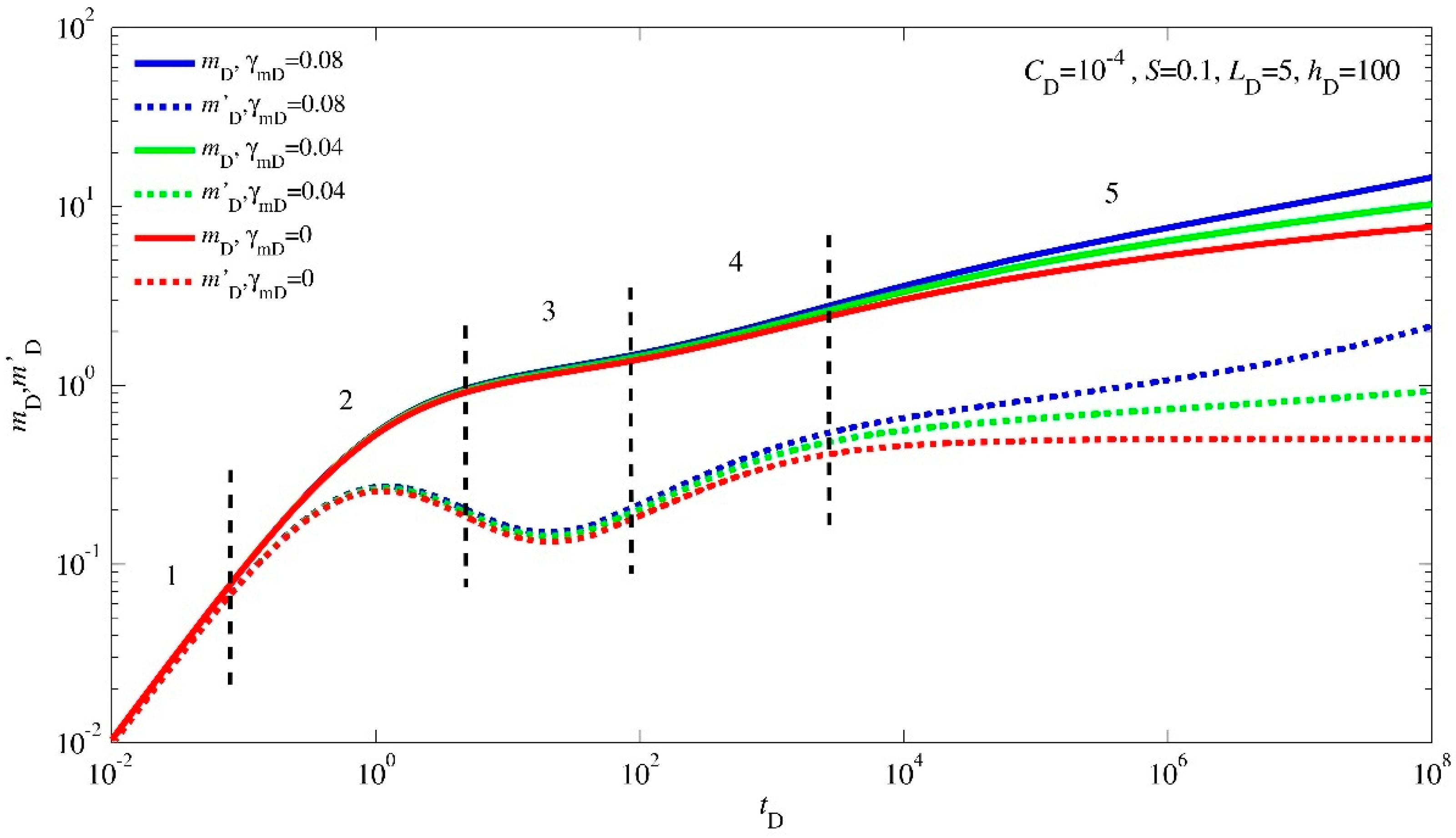
3.1. Flow Periods Recognition of Type Curves

Figure 2 displays the transient pressure dynamics of a horizontal well in an infinitely large abnormally high-pressure gas reservoir, considering the effects of stress-sensitivity. In the context of Figure 2, the red curves illustrate the scenario where stress-sensitivity is not considered, offering a lucid depiction of unique features throughout each time phase. The subsequent explanation delineates the fundamental characteristics of the five predominant flow regimes.

Phase 1: Pure wellbore storage effect flow phase. The pressure curves and their derivatives coincide, forming a rising line with a gradient of “1”. Phase 2: Transition phase influenced by the skin effect. The pressure derivative curve takes on a “hump” shape. Phase 3: Early radial flow phase in the vertical plane. The derivative curve remains a horizontal straight line, with a magnitude linked to L_D. This stage portrays the radial flow pattern perpendicular to the horizontal axis prior to the propagation of pressure waves to the upper and lower outer boundaries. Phase 4: Mid-term linear flow phase. The derivative curve forms a rising straight line with a slope of “1/2”. Phase 5: Late pseudo-radial flow phase. The derivative curve becomes a horizontal line positioned at 0.5 on the y-axis.

3.2. Sensitivity Analysis of Transient Pressure Dynamics

3.2.1. Effect of Permeability Modulus

Figure 2 also illustrates the influence of the permeability modulus on the characteristic curves of transient pressure behavior. This influence is particularly pronounced in the final flow regime, where, when γ_mD = 0, the derivative curves remain horizontal at a value of 0.5 on the y-axis. As the value of γ_mD escalates, a series of distinct modifications emerge within the derivative curves. A gradual and progressive upward tilt becomes evident, signifying a profound alteration in the behavior of the fluid within the reservoir. This upward shift in the derivative curves mirrors the growing influence of stress-sensitivity, a phenomenon in which permeability undergoes heightened disruption due to external forces or pressure effects.

The correlation between γ_mD values and stress-sensitivity reveals a compelling trend. Higher values of γ_mD, signaling increased stress-sensitivity, lead to a heightened degree of permeability impairment. Consequently, the fluid flow encounters greater resistance within the reservoir, necessitating the application of more substantial drawdown pressures to facilitate effective production.

Through this exploration, Figure 2 emerges as a valuable analytical tool, unveiling the multifaceted interactions between the permeability modulus, stress-sensitivity, and pressure dynamics. It encapsulates the story of how even subtle changes in these factors can result in significant alterations in transient pressure behavior, unveiling insights critical to reservoir characterization and production strategy.

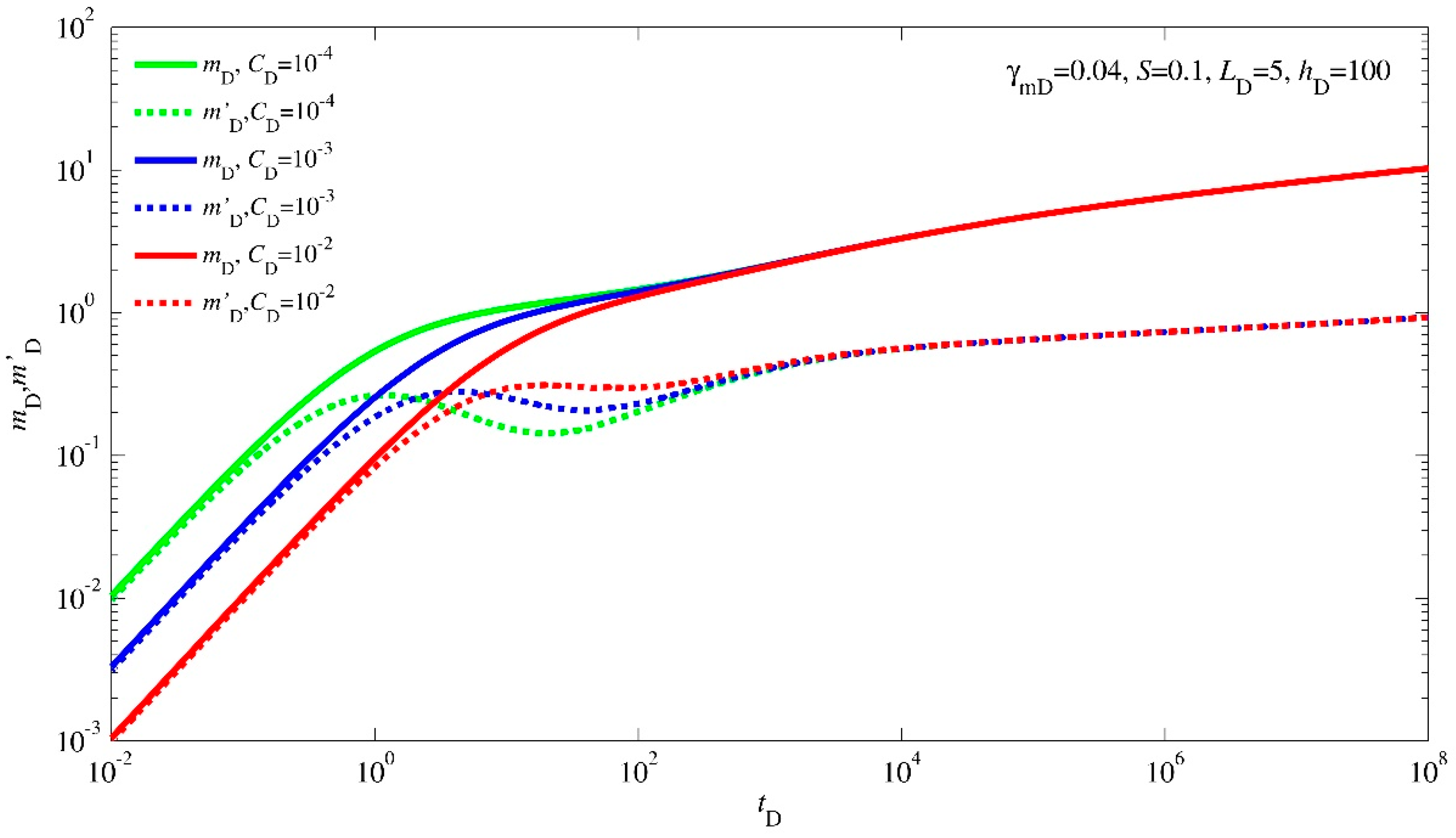
3.2.2. Effect of Wellbore Storage Coefficient

Figure 3 provides insight into how the wellbore storage coefficient influences the characteristics of transient pressure response type curves. Initially, an elevated wellbore storage coefficient translates into an extended lifespan for the wellbore storage phase. This extension arises from the increased capacity of the wellbore to store fluids, thus impacting the early stages of the pressure response.

Equally noteworthy is the consequential reduction in the prominence of the skin effect hump within the derivative curve. This phenomenon signifies a modulation in the skin effect, which is a measure of near-wellbore damage or alterations in the fluid flow. A more substantial wellbore storage phase mitigates the influence of the skin effect, leading to a less conspicuous “hump” in the derivative curve during the transition phase. However, it is essential to recognize that a delicate balance is at play. As the wellbore storage coefficient magnifies, so too does the potential for an intriguing outcome: the possible concealment of the vertical radial flow regime, once a certain critical value of C_D is surpassed.

This interplay of factors emphasizes the nuanced nature of reservoir dynamics and the role of the wellbore storage coefficient as a key orchestrator. Figure 3 thus stands as an invaluable visual aid, shedding light on the interwoven relationship between the wellbore storage coefficient and the progression of transient pressure behavior. Through these insights, it offers a pathway to refined analyses, better reservoir management, and enhanced production strategies.

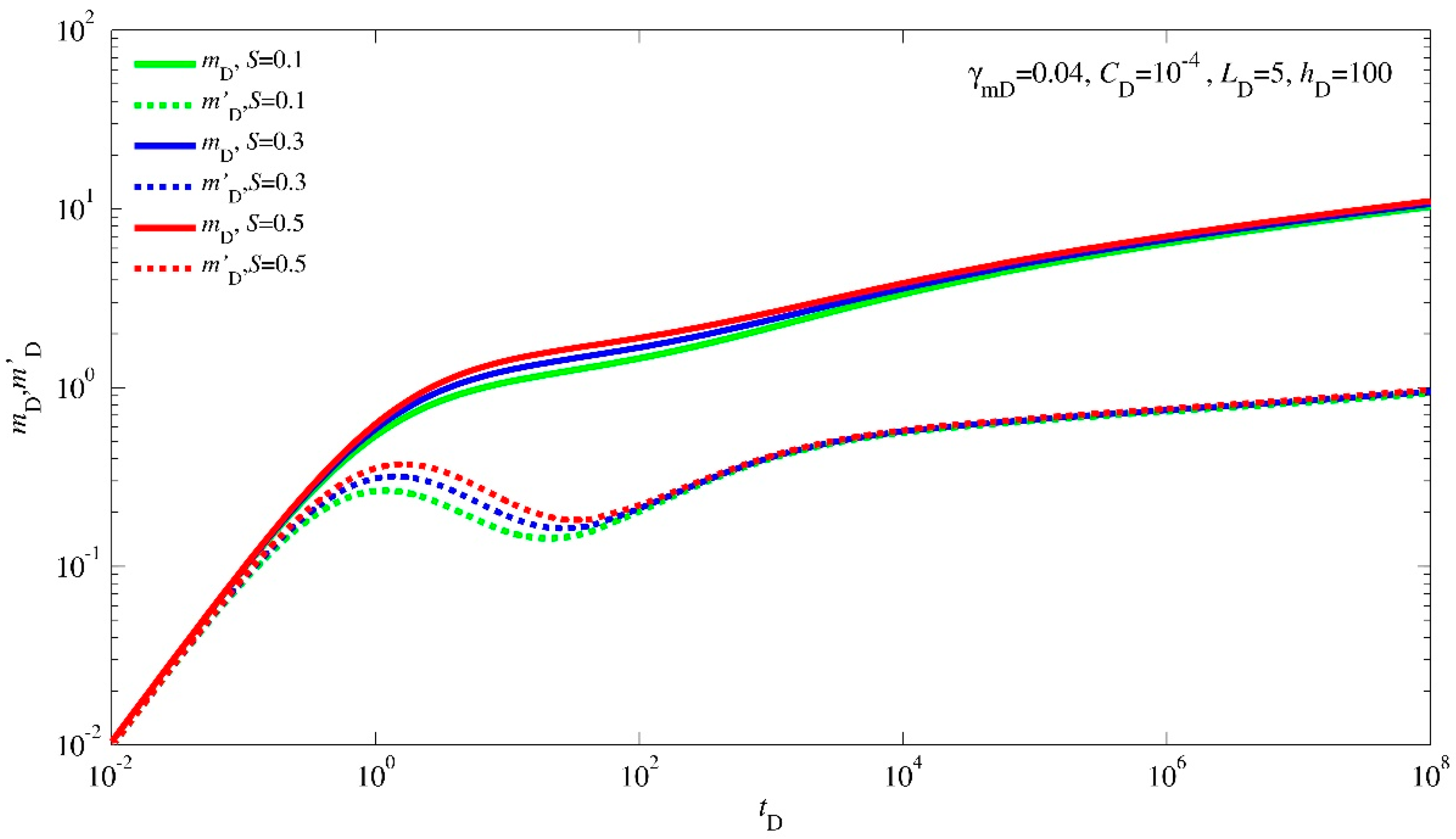
3.2.3. Effect of Skin Factor

Figure 4 depicts the effect of the skin factor on transient pressure behavior type curves. This influence primarily manifests itself in the morphology of the type curves during the transition phase (Period 2) that follows the wellbore storage period. As the skin factor value escalates, a notable alteration occurs in the positioning of the “hump” within the derivative curves, leading to its elevation. This upward shift signifies a more substantial additional pressure drop taking place in the formation.

This phenomenon highlights the intricate relationship between the skin factor and the dynamic flow characteristics within the reservoir. The shift of the “hump” underscores how the skin factor can impact the flow resistance near the wellbore, consequently influencing the overall pressure behavior as the well transitions from the wellbore storage phase to the subsequent flow regimes.

Understanding and analyzing the interplay between the skin factor and the pressure behavior type curves is pivotal for optimizing production strategies. A higher skin factor can signify challenges in the reservoir connectivity and fluid flow, necessitating careful consideration during well design and reservoir management decisions. Consequently, Figure 4 serves as a valuable visual aid in comprehending the nuanced effects of the skin factor on transient pressure dynamics.

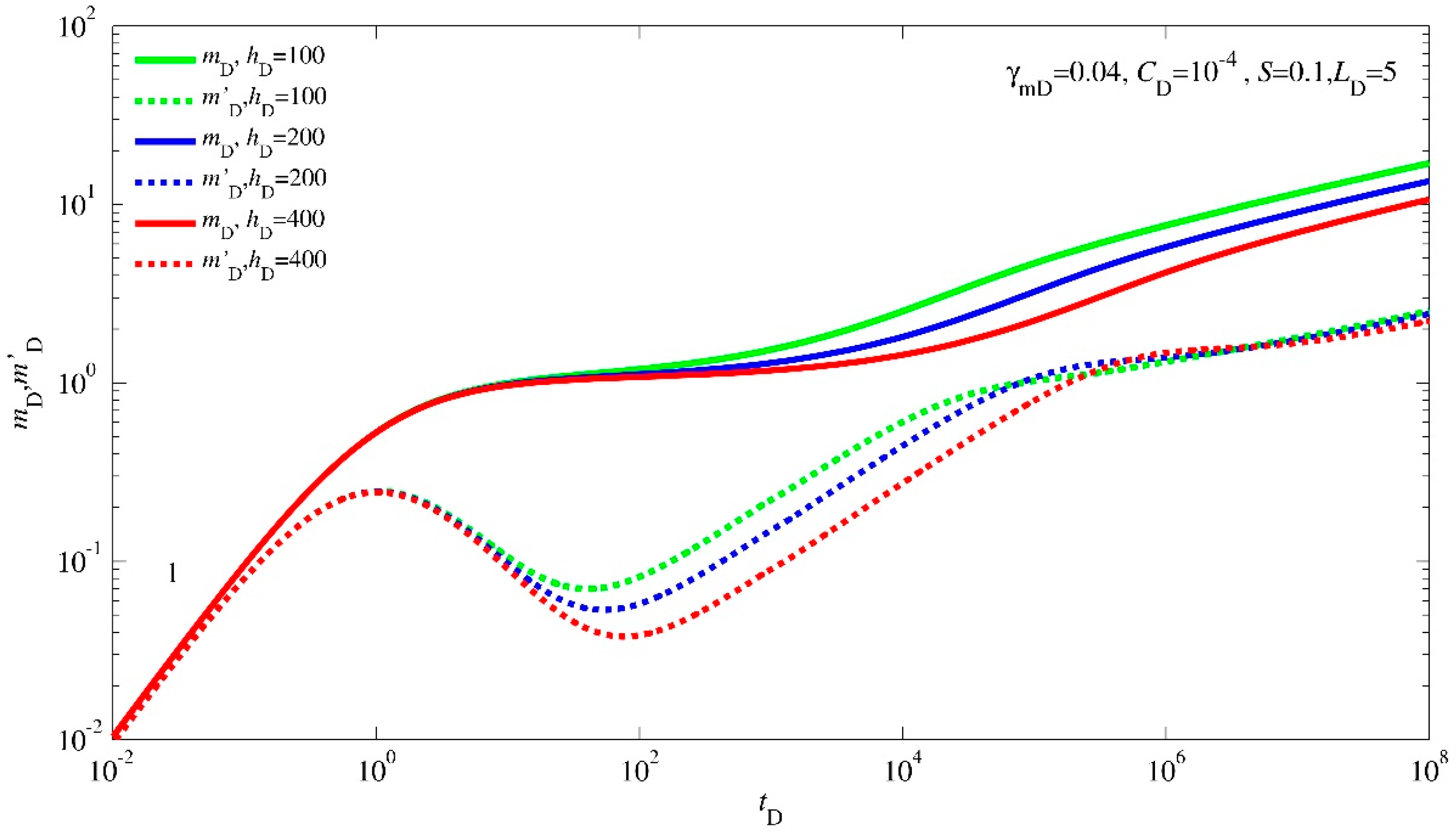
3.2.4. Effect of Reservoir Thickness

Figure 5 offers a comprehensive perspective on how reservoir thickness influences the transient pressure behavior type curves. As the reservoir thickness augments, a compelling consequence emerges: the time required for the pressure wave to traverse to both the upper and lower boundaries of the reservoir extends significantly. This phenomenon is a direct result of the increased distance that the pressure wave needs to travel before encountering these outer limits. The consequence of this prolonged propagation time is manifold, reshaping the temporal progression of various flow regimes.

The early vertical radial flow regime experiences an elongated duration. Then, the mid-term linear flow phase, which normally follows the vertical radial flow regime, is naturally delayed. The increased propagation time introduces a lag in the initiation of this flow regime, impacting the timing and duration of the linear flow behavior. Lastly, the late pseudo-radial flow stage, which marks the final phase of transient pressure behavior, also encounters a delay.

Figure 5 offers valuable insights into the intricate interplay between reservoir thickness and transient pressure behavior. The alterations in propagation time due to changes in reservoir thickness create a cascading effect that reverberates through various flow regimes, ultimately contributing to a more holistic understanding of reservoir dynamics and aiding in strategic decision-making for reservoir management and well operation.

4. Conclusions

In this study, a comprehensive mathematical framework is meticulously developed to accommodate the intricate interplay of stress-sensitivity for a horizontal well nestled in tight gas reservoirs. In addition, this model provides a robust foundation for scrutinizing the transient flow behaviors inherent in such scenarios. The ensuing outcomes can be succinctly encapsulated as follows:

• The developed model, adept at delineating the intricate fluid flow influenced by stress-sensitivity, is introduced as a tool for dissecting the transient pressure dynamics in horizontal wells situated within abnormally high-pressure tight gas reservoirs. Compared with the conventional well testing interpretation tool, the established model can better explain the permeability parameters in such a formation and be more in line with the actual situation.
• An approximate analytical solution for pressure responses in the Laplace domain is generated by systematically integrating Pedrosa’s linearization techniques, perturbation methodology, Laplace transformations, Sturm–Liouville eigenvalue theory, and orthogonal transformations. This will provide valuable inspiration for further expansions to complex well types, complex geological conditions, or complex flow phases.
• Stress-sensitivity, an indicator of the formation permeability damage, engenders amplified pressure drops during the intermediate and late flow stages. These pronounced pressure drops find expression through discernible upward trends observed in both pressure and production derivative curves.
• The influence of other parameters, such as the wellbore storage coefficient, skin factor, and reservoir thickness, on the transient flow dynamics closely parallels the behavior observed in conventional gas reservoirs.

By synergistically incorporating these methodologies, the model not only deepens our understanding of the behavior of horizontal wells within tight gas reservoirs influenced by stress-sensitivity but also enriches the broader discourse on transient flow phenomena in petroleum engineering. Next, this paper can be extended to model research on fractured horizontal wells, gas-water two-phase flow, multiple media, and even coupled formation with threshold pressure gradients, etc., thus continuously strengthening the in-depth understanding of the seepage law of tight gas reservoirs.

References

1. Faramawy, S.; Zaki, T.; Sakr, A.-E. Natural gas origin, composition, and processing: A review. J. Nat. Gas Sci. Eng. 2016, 34, 34–54. [Google Scholar] [CrossRef]
2. Reyna, J.L.; Chester, M.V. Energy efficiency to reduce residential electricity and natural gas use under climate change. Nat. Commun. 2017, 8, 14916. [Google Scholar] [CrossRef] [PubMed]
3. Hou, Z.; Luo, J.; Cao, C.; Ding, G. Development and contribution of natural gas industry under the goal of carbon neutrality in China. Adv. Eng. Sci. 2023, 55, 243–252. [Google Scholar]
4. Dormieux, L.; Jeannin, L.; Gland, N. Homogenized models of stress-sensitive reservoir rocks. Int. J. Eng. Sci. 2011, 49, 386–396. [Google Scholar] [CrossRef]
5. Zhao, L.; Chen, Y.; Ning, Z.; Wu, X.; Liu, L.; Chen, X. Stress sensitive experiments for abnormal overpressure carbonate reservoirs: A case from the Kenkiyak fractured-porous oil field in the littoral Caspian Basin. Pet. Explor. Dev. Online 2013, 40, 208–215. [Google Scholar] [CrossRef]
6. Liu, Z.; Zhao, J.; Kang, P.; Zhang, J. An experimental study on simulation of stress sensitivity to production of volcanic gas from its reservoir. J. Geol. Soc. India 2015, 86, 475–481. [Google Scholar] [CrossRef]
7. Tan, X.-H.; Li, X.-P.; Liu, J.-Y.; Zhang, G.-D.; Zhang, L.-H. Analysis of permeability for transient two-phase flow in fractal porous media. J. Appl. Phys. 2014, 115, 113502. [Google Scholar] [CrossRef]
8. Tan, X.-H.; Li, X.-P.; Liu, J.-Y.; Zhang, L.-H.; Fan, Z. Study of the effects of stress sensitivity on the permeability and porosity of fractal porous media. Phys. Lett. A 2015, 379, 2458–2465. [Google Scholar] [CrossRef]
9. Tian, X.; Cheng, L.; Cao, R.; Wang, Y.; Zhao, W.; Yan, Y.; Liu, H.; Mao, W.; Zhang, M.; Guo, Q. A new approach to calculate permeability stress sensitivity in tight sandstone oil reservoirs considering micro-pore-throat structure. J. Pet. Sci. Eng. 2015, 133, 576–588. [Google Scholar] [CrossRef]
10. Wang, S.; Ma, M.; Ding, W.; Lin, M.; Chen, S. Approximate analytical-pressure studies on dual-porosity reservoirs with stress-sensitive permeability. SPE Reserv. Eval. Eng. 2015, 18, 523–533. [Google Scholar] [CrossRef]
11. Wenlian, X.; Tao, L.; Min, L.; Jinzhou, Z.; Zheng, L.; Ling, L. Evaluation of the stress sensitivity in tight reservoirs. Pet. Explor. Dev. 2016, 43, 115–123. [Google Scholar]
12. Hamid, O.; Osman, H.; Rahim, Z.; Omair, A. Stress dependent permeability of carbonate rock. In Proceedings of the SPE Annual Technical Conference and Exhibition, Indianapolis, IN, USA, 23–25 May 2016; OnePetro: Richardson, TX, USA, 2016. [Google Scholar]
13. Raghavan, R.; Chin, L.Y. Productivity changes in reservoirs with stress-dependent permeability. In Proceedings of the SPE Annual Technical Conference and Exhibition, San Antonio, TX, USA, 29 September–2 October 2002; SPE: Kuala Lumpur, Malaysia, 2002; p. SPE-77535-MS. [Google Scholar] [CrossRef]
14. Fang, Y.; Yang, B. Application of new pseudo-pressure for deliverability test analysis in stress-sensitive gas reservoir. In Proceedings of the SPE Asia Pacific Oil and Gas Conference and Exhibition, Jakarta, Indonesia, 4–6 August 2009; SPE: Kuala Lumpur, Malaysia, 2009; p. SPE-120141-MS. [Google Scholar]
15. Lian, P.; Cheng, L.; Liu, L. Characteristics of Productivity Curves in Abnormal High-Pressure Reservoirs. Pet. Sci. Technol. 2011, 29, 109–120. [Google Scholar] [CrossRef]
16. Dou, X.; Liao, X.; Zhao, X.; Wang, H.; Lv, S. Quantification of permeability stress-sensitivity in tight gas reservoir based on straight-line analysis. J. Nat. Gas Sci. Eng. 2015, 22, 598–608. [Google Scholar] [CrossRef]
17. Celis, V.; Silva, R.; Ramones, M.; Guerra, J.; Da Prat, G. A new model for pressure transient analysis in stress sensitive naturally fractured reservoirs. SPE Adv. Technol. Ser. 1994, 2, 126–135. [Google Scholar] [CrossRef]
18. Zhang, M.; Ambastha, A. New insights in pressure-transient analysis for stress-sensitive reservoirs. In Proceedings of the SPE Annual Technical Conference and Exhibition, New Orleans, LA, USA, 25–28 September 1994; SPE: Kuala Lumpur, Malaysia, 1994; p. SPE-28420-MS. [Google Scholar]
19. Jelmert, T.; Selseng, H. Pressure transient behavior of stress-sensitive reservoirs. In Proceedings of the SPE Latin America and Caribbean Petroleum Engineering Conference, Rio de Janeiro, Brazil, 30 August–3 September 1997; SPE: Kuala Lumpur, Malaysia, 1997; p. SPE-38970-MS. [Google Scholar] [CrossRef]
20. Pinzon, C.L.; Chen, H.-Y.; Teufel, L.W. Numerical well test analysis of stress-sensitive reservoirs. In Proceedings of the SPE Rocky Mountain Petroleum Technology Conference, Keystone, CO, USA, 21–23 May 2001; OnePetro: Richardson, TX, USA, 2001. [Google Scholar]
21. Archer, R. Impact of stress sensitive permeability on production data analysis. In Proceedings of the SPE Unconventional Resources Conference/Gas Technology Symposium, Calgary, AB, Canada, 10–12 February 2008; SPE: Kuala Lumpur, Malaysia, 2008; p. SPE-114166-MS. [Google Scholar] [CrossRef]
22. Yao, S.; Zeng, F.; Liu, H.; Zhao, G. A semi-analytical model for multi-stage fractured horizontal wells. In Proceedings of the SPE Canadian Unconventional Resources Conference, Calgary, AB, Canada, 30 October–1 November 2012; OnePetro: Richardson, TX, USA, 2012. [Google Scholar]
23. Pedrosa Jr, O.A. Pressure transient response in stress-sensitive formations. In Proceedings of the SPE Western Regional Meeting, Oakland, CA, USA, 2–4 April 1986; SPE: Kuala Lumpur, Malaysia, 1986; p. SPE-15115-MS. [Google Scholar] [CrossRef]
24. Kikani, J.; Pedrosa, O.A., Jr. Perturbation analysis of stress-sensitive reservoirs. SPE Form. Eval. 1991, 6, 269–379. [Google Scholar] [CrossRef]
25. Guo, J.; Wang, H.; Zhang, L.; Li, C. Pressure transient analysis and flux distribution for multistage fractured horizontal wells in triple-porosity reservoir media with consideration of stress-sensitivity effect. J. Chem. 2015, 2015, 212901. [Google Scholar] [CrossRef]
26. Zeng, F.; Zhao, G. Well testing analysis for variable permeability reservoirs. J. Can. Pet. Technol. 2007, 46. [Google Scholar] [CrossRef]
27. Xiao, X.; Sun, H.; Han, Y.; Yang, J. Dynamic characteristic evaluation methods of stress sensitive abnormal high pressure gas reservoir. In Proceedings of the SPE Annual Technical Conference and Exhibition, New Orleans, LA, USA, 4–7 October 2009; SPE: Kuala Lumpur, Malaysia, 2009; p. SPE-124415-MS. [Google Scholar]
28. Qanbari, F.; Clarkson, C.R. Rate transient analysis of stress-sensitive formations during transient linear flow period. In Proceedings of the SPE Canada Unconventional Resources Conference, Calgary, AB, Canada, 30 October–1 November 2012; SPE: Kuala Lumpur, Malaysia, 2009; p. SPE-162741-MS. [Google Scholar]
29. Cai, J.; Yu, B. A discussion of the effect of tortuosity on the capillary imbibition in porous media. Transp. Porous Media 2011, 89, 251–263. [Google Scholar] [CrossRef]
30. Cai, J.-C. A fractal approach to low velocity non-Darcy flow in a low permeability porous medium. Chin. Phys. B 2014, 23, 044701. [Google Scholar] [CrossRef]
31. Wang, F.; Li, X.; Couples, G.; Shi, J.; Zhang, J.; Tepinhi, Y.; Wu, L. Stress arching effect on stress sensitivity of permeability and gas well production in Sulige gas field. J. Pet. Sci. Eng. 2015, 125, 234–246. [Google Scholar] [CrossRef]
32. Ding, J.; Yang, S.; Cao, T.; Wu, J. Dynamic threshold pressure gradient in tight gas reservoir and its influence on well productivity. Arab. J. Geosci. 2018, 11, 783. [Google Scholar] [CrossRef]
33. Wu, Z.; Cui, C.; Trivedi, J.; Ai, N.; Tang, W. Pressure analysis for volume fracturing vertical well considering low-velocity non-Darcy flow and stress sensitivity. Geofluids 2019, 2019, 2046061. [Google Scholar] [CrossRef]
34. Chu, H.; Ma, T.; Zhu, W.; Gao, Y.; Zhang, J.; Lee, W.J. A novel semi-analytical monitoring model for multi-horizontal well system in large-scale underground natural gas storage: Methodology and case study. Fuel 2023, 334, 126807. [Google Scholar] [CrossRef]
35. Xu, Y.; Tan, X.; Li, X.; Li, J.; Liu, Q. Blasingame production decline and production prediction model of inclined well in triple-porosity carbonate gas reservoir. J. Nat. Gas Sci. Eng. 2021, 92, 103983. [Google Scholar] [CrossRef]
36. Van Everdingen, A. The skin effect and its influence on the productive capacity of a well. J. Pet. Technol. 1953, 5, 171–176. [Google Scholar] [CrossRef]
37. Kucuk, F.; Ayestaran, L. Analysis of simultaneously measured pressure and sandface flow rate in transient well testing (includes associated papers 13,937 and 14,693). J. Pet. Technol. 1985, 37, 323–334. [Google Scholar] [CrossRef]
38. Stehfest, H. Algorithm 368: Numerical inversion of Laplace transforms [D5]. Commun. ACM 1970, 13, 47–49. [Google Scholar] [CrossRef]
Figure 1. Illustration showcasing a horizontal gas well situated in a formation.
Energies 16 07175 g001
Figure 2. Flow regimes of the transient pressure dynamics affected by permeability modulus.
Energies 16 07175 g002
Figure 3. Type curves of the transient pressure response affected by wellbore storage coefficient.
Energies 16 07175 g003
Figure 4. Type curves of the transient pressure response affected by skin factor.
Energies 16 07175 g004
Figure 5. Type curves of the transient pressure response affected by reservoir thickness.
Energies 16 07175 g005