Article

Multi-Scale Seismic Measurements for Site Characterization and CO2 Monitoring in an Enhanced Oil Recovery/Carbon Capture, Utilization, and Sequestration Project, Farnsworth Field, Texas

by
George El-kaseeh
1 and
Kevin L. McCormack
2,*
1
Petroleum Resource Recovery Center, New Mexico Institute of Mining and Technology, Socorro, NM 87801, USA
2
Energy and Geoscience Institute, University of Utah, Salt Lake City, UT 84112, USA
*
Author to whom correspondence should be addressed.
Energies 2023, 16(20), 7159; https://doi.org/10.3390/en16207159
Submission received: 9 September 2023 / Revised: 12 October 2023 / Accepted: 18 October 2023 / Published: 19 October 2023
(This article belongs to the Special Issue Forecasting CO2 Sequestration with Enhanced Oil Recovery II)

Abstract

:
To address the challenges of climate change, significantly more geologic carbon sequestration projects are beginning. The characterization of the subsurface and the migration of the plume of supercritical carbon dioxide are two elements of carbon sequestration that can be addressed through the use of the available seismic methods in the oil and gas industry. In an enhanced oil recovery site in Farnsworth, TX, we employed three separate seismic techniques. The three-dimensional (3D) surface seismic survey required significant planning, design, and processing, but produces both a better understanding of the subsurface structure and a three-dimensional velocity model, which is essential for the second technique, a timelapse vertical seismic profile, and the third technique, cross-well seismic tomography. The timelapse 3D Vertical Seismic Profile (3D VSP) revealed both significant changes in the reservoir between the second and third surveys and geo-bodies that may represent the extent of the underground carbon dioxide. The asymmetry of the primary geo-body may indicate the preferential migration of the carbon dioxide. The third technique, cross-well seismic tomography, suggested a strong correlation between the well logs and the tomographic velocities, but did not observe changes in the injection interval.

1. Introduction

Geophysical methods that employ active sources (i.e., Vibroseis or/and explosives) play an important role in hydrocarbon exploration and production [1,2]. Geophysical measurements are used to image subsurface geological structures and identify potential hydrocarbon-bearing reservoirs. In the past few decades, several geophysical data acquisition, processing, and interpretation technologies were developed by the oil and gas industry to identify reservoirs, optimize production, and the reduce cost of hydrocarbon extraction [3,4,5,6]. Some of these technologies have been adopted by Carbon Capture and Sequestration (CCS) and Carbon Capture, Utilization, and Sequestration (CCUS) projects. Enhanced oil recovery (EOR) is a technology that uses supercritical carbon dioxide to dissolve oil, reducing its viscosity and allowing for greater production [7,8]. The success of EOR both as a means to produce more oil and sequester carbon dioxide is dependent on careful site characterization and the available pipeline infrastructure [9,10,11]. CCS and CCUS projects utilize geophysical methods for site and reservoir characterization, and injected CO2 plume development, migration, and containment monitoring [12]. The Farnsworth Unit (FWU) is a CCUS project where geophysical methods were implemented as part of a comprehensive Monitoring, Verification and Accounting (MVA) program [13,14]. In this paper, the geophysical methods specific to the FWU will be discussed in detail.
While designing the monitoring schedule at the FWU, we considered several elements: the expected evolution of the position and the size of the CO2 plume; the areal extent of the pressure plume; the depth and thickness of the primary reservoir, which is important for storage potential; the current and proposed characterization work of the caprock integrity; and the sensitivity of various geophysical measurements to the field conditions.
The geophysical monitoring included a high-resolution three-dimensional surface seismic survey to improve the interpretation of structure, as well as to support the estimation of the storage capacity. The surface three-dimensional data were also used to map the lithology and petrophysical properties based on the inversion of the seismic data. Three-dimensional VSP and cross-well seismic surveys were acquired to enhance the understanding of the geologic detail, especially in the vicinity of the well. Some of the surveys were acquired prior to the injection of the supercritical carbon dioxide, and these surveys provide a baseline for the time-lapse (4D) monitoring.
The different seismic techniques that are available cover different scales and dimensions of investigation. For instance, three-dimensional surface seismic surveys provide observations of a large region beneath the survey, and conversely, cross-well seismic tomography generates a two-dimensional velocity field between wells. By combining several types of techniques, the greatest lateral and vertical resolution of the subsurface can be acquired. In order to avoid interfering with the agricultural season, the seismic surveys were conducted in the winter months, which meant that the measurements were taken over a four-year period. Three geophysical technologies were employed at the FWU: (1) a three-dimensional surface seismic survey; (2) three-dimensional VSP surveys at wells planned for conversion to CO2 injectors; and (3) cross-well seismic profiles between pairs of wells, including one which was planned for conversion to CO2 injection. The baseline and monitor VSP and cross-well seismic surveys were acquired at the same time of year (winter), to ensure high repeatability and reduce uncertainty in the time-lapse analyses. This paper details the acquisition and processing of each of the three techniques within the context of understanding the evolution of the plume of injected supercritical carbon dioxide.

2. 3D Surface Seismic

2.1. Data Acquisition

The high-density 3D field-scale surface seismic survey was acquired in 2013. Improving the field-scale structural and stratigraphic interpretation, the survey provided an estimation of storage capacity and geomechanical properties. The surface area of the survey covered approximately a 108.8 km2 (42 m2) total surface area and a 69.9 km2 (27 m2) full fold area (Figure 1). The project team carefully developed a survey evaluation and design (SED). The planning and design took into consideration the existing infrastructure and the project’s imaging objectives. A result of the SED was a geometry file that predicted the optimal locations for the sources and receivers as well as a timeline for the efficient progression of the fieldwork. Also, as part of the SED, field testing was conducted to maximize the results of the source parameters from the Vibroseis. Careful quality control was applied throughout the duration of data acquisition in the FWU.
The target reservoir, the Morrow B, is a thin sandstone layer [15], which implies that a high lateral and vertical resolution is required. The density of the sources and receivers dictates the degree of resolution available in the survey. Thus, a high density is required for our objectives [16]. Based on the results of the field testing, a broad-band (2 Hz–100 Hz) non-linear Vibroseis sweep was designed, which has an appropriate frequency content to obtain the desired resolution. Although our frequency range is developed to image the thin Morrow B formation, a low-frequency rich dataset can accurately provide a pre-stack elastic inversion. The sweep was designed to enhance low frequencies (below 10 Hz) that are important for seismic inversion objectives. Receiver lines consisting of dense point receivers at 33-foot spacing were deployed, which help to preserve the higher frequencies that are needed for the survey to be sensitive to thin layers. Also, the high frequencies aid in modeling and subtracting unaliased noise.
To ensure that the survey adhered to the acquisition geometry parameters generated through the SED study, daily geometry quality control was performed in the field. Any necessary adjustments due to unforeseen changes in infrastructure near the survey area were made in real time. The geometry attributes were recalculated to verify that adequate subsurface coverage was maintained (Figure 2). Additionally, multiple attributes were computed and analyzed to verify the integrity of the field seismic data. We will present the results along the 1925 inline, but the generalized outcomes can be extrapolated to the entire three-dimensional volume.

2.2. Data Processing

Numerous processing techniques were employed on the seismic gathers using Schlumberger’s proprietary data processing software, Omega® version 2. These techniques enabled the operators to discern different characteristics about the site from the same raw waveforms. In some cases, if the data are processed in only one way, certain key elements of the structure and geology of the site may be overlooked. The first processing method was traditional time domain processing, which involves the least perturbation to the original waveforms. The processing flow was designed to preserve the relative magnitudes of different seismic traces and accurately generate a 3D seismic volume that allows for structural interpretation and reservoir characterization. Noise, whether source-generated (coherent) or wind (ambient), and near-surface irregularities within the survey area (statics) were overcome by the processing workflow (Table 1). Noise was attenuated through the modeling and adaptive subtraction techniques of unaliased noise in multiple domains. Near-surface irregularities caused data samples to appear at the incorrect time within a trace as well as the misalignment of traces within a shot gather. In order to address this problem, and to assure convergence on a valid statics solution, first-break picking was performed manually on the point receiver shots and receiver gathers.
The second processing technique was the conversion of the seismic volume into the depth domain by means of a velocity model, which improves the ability to image the Morrow B reservoir interval. For the initial near-surface model building, refraction tomography velocities were used. The sediment velocity model, a product of time processing, was first used while building the initial velocity model, in combination with the shallow refraction tomography velocities. Check-shot velocities from a single well location (13-10A) were used to populate the deeper section of the model (from the VSP model). In addition, common image point (CIP) tomography was used to update the velocity model after applying three noise attenuation techniques: Anomalous Amplitude Attenuations (AAA), 3D Matching Pursuit Noise Attenuation (MPNA), and Curvelet Transform.
Data were partitioned via Offset Vector Tiles (OVTs) binning, an industry-accepted approach to splitting wide and full-azimuth long-offset data prior to imaging, as a means of maintaining the azimuthal response in the data for later attribute extraction, including Azimuthal Amplitude Versus Offset (AVOAz) inversion and velocity azimuthal variation. In order to reduce migration artifacts due to the existence of empty cells within each OVT volume, a cascaded interpolation algorithm approach was used in order to fill empty cells or gaps in the OVT domain. First, Reciprocal OVT Gap Fill was used for each two reciprocal OVTs, then Matching Pursuit Fourier Interpolation (3D-MPFI) was used to further fill the gaps within a limited distance.
Since the depth model that is anisotropic with respect to the body wave velocities is relatively simple to construct, the majority of our processing is concentrated on the anisotropic model, which contains more detail of the structure of the subsurface. Anisotropy can be described using Thomsen’s [17] parameters of epsilon and delta. In the case of the Farnsworth Unit, these two parameters, which represent the horizontal and vertical interactions of velocity, respectively, are shown to vary in a one-dimensional manner with depth (Figure 3). Using the anisotropic approach, offsets in the stratigraphy were flattened both in the central portion of the model as well as toward the edges.
The computationally expensive common image point (CIP) tomography further enhances the model by updating the velocity model in an iterative manner. The approach is to converge over a series of iterations towards a solution with the smoothness constraints relaxed from iteration to iteration. The most well-determined, long-wavelength features are solved for first, and the least-determined, short-wavelength features are solved for last. For each iteration, drastic updates were avoided to avoid violating the linear, fixed-ray path assumptions of the tomographic equations. Typically, decreasing the scale length is stopped when the objective function is reduced by about 20% and the velocities are changed by about 10%. The starting velocity model is typically smoothed, since short-wavelength inaccuracies in the initial model can introduce instabilities in the method. The full workflow of the CIP tomography can be seen in Figure 4, and the results after four iterations can be seen in Figure 5.

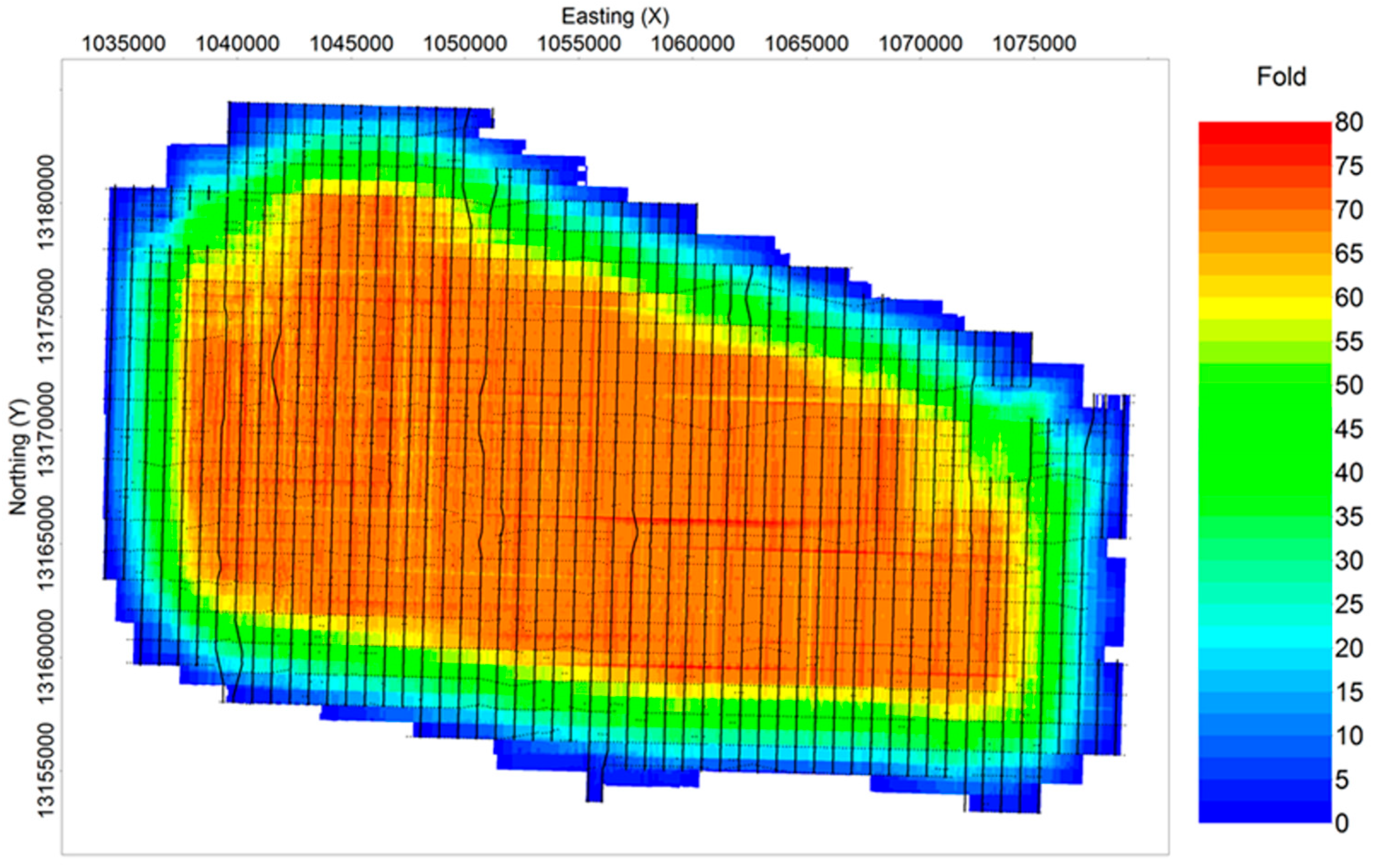
2.3. Results of the 3D Survey

Additional improvements to the model included Kirchhoff pre-stack depth migration, which sums weighted amplitudes along diffraction curves; principle component reconstruction noise attenuation, which enhances the signal-to-noise ratio of the traces; spatially continuous velocity analysis, which assists in interpolating data between grid nodes; residual event alignment, which helps to flatten migrated gathers; and spatially residual amplitude correction, which removes many of the concave-up parabolas that can be an artifact of the processing. The composite image of all these methods is shown in Figure 6. This model represents the most complete understanding of the three-dimensional seismic survey.

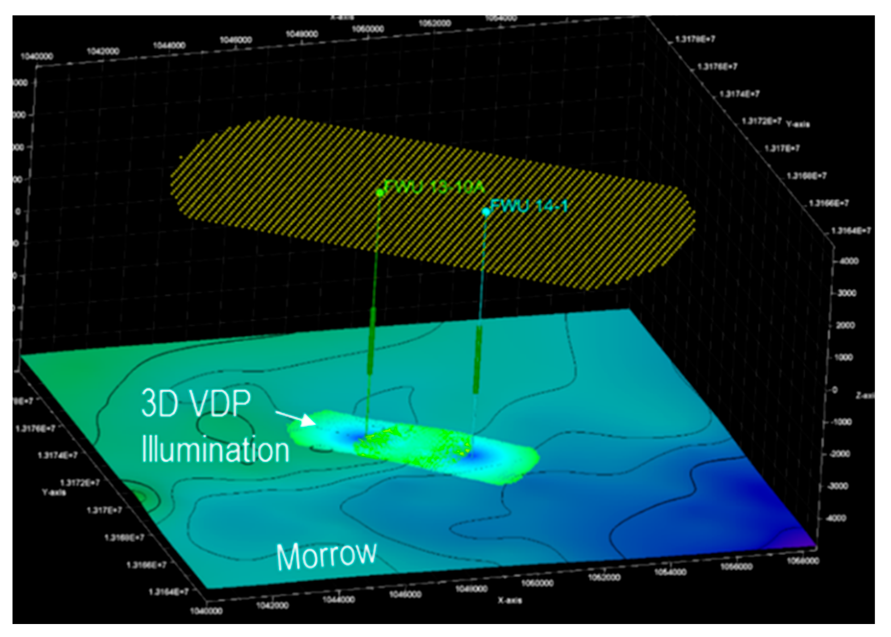
3. Vertical Seismic Profile

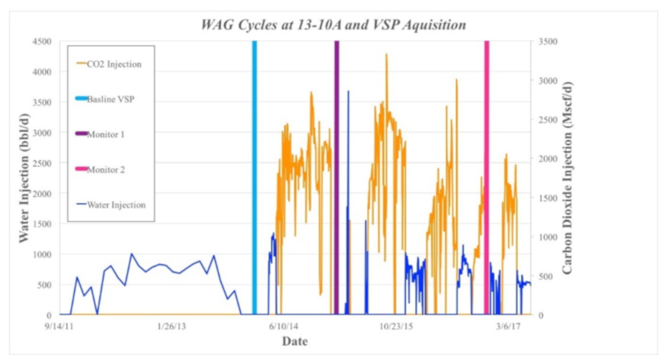
3.1. Data Acquisition

Two baseline 3D vertical seismic profile (VSP) surveys for two wells were acquired simultaneously in 2014 (wells 13-10A and 14-01), as well as a third one in 2015 (well 32-08). Two monitor (time-lapse) surveys for well 13-10A were acquired in January 2015 (33,070.25 tons of CO2 injected) and November 2016 (76,596.64 tons CO2 injected). The proximity of wells 13-10A and 14-01 presented the opportunity for simultaneous data acquisition. Ray-tracing-based survey evaluation and design (SED) was conducted for the baseline surveys of the two wells to optimize the acquisition parameters as well as to reduce the data acquisition, processing time, and cost. The SED produced a geometry file with source locations that reflected the maximum usable offset distance. The simultaneous data acquisition reduced the number of source points acquired by 2100 points (42%). Illumination maps (hit maps) were generated and analyzed to verify that the target horizon (Morrow B) was adequately illuminated (Figure 7).
The acquisition parameters were determined based on analyses of the results from the SED study. Optimal survey planning was determined based on the existing infrastructure and accessibility within the survey area. For operational reasons and to minimize negative impacts on oil production, the data acquisition for the three surveys was coordinated with the field operator to coincide with the water injection period of the water-alternating-gas (WAG) cycle (Figure 8).
To ensure repeatability and reduce uncertainty in the time-lapse analysis, source locations from the baseline survey for well 13-10A were repeated for the two monitor surveys using the same downhole tool and source parameters. In the early stages of processing, co-located sources from the three surveys were selected for subsequent processing.

3.2. Data Processing

The 3D VSP baseline data for each of the three wells were independently processed. For well 13-10A, data from the baseline and monitor surveys were processed through an identical three-component (3C) processing workflow. The pre-processing included filling source/receiver geometry using information from a field report, receiver selection, 3C orientation, noise attenuation, Surface-Consistent Amplitude Compensation (SCAC), 3C wavefield separation, deterministic trace-by-trace wave-shaping deconvolution, and static correction. This section focuses on the processing of the baseline and time-lapse surveys for well 13-10A. The time-lapse (4D) analyses will be discussed in Section 3.3.1.
In order to minimize differences due to variation in the acquisition geometries of the surveys, only the co-located shot points with receivers in good quality for the three surveys were used in the time-lapse processing. The source point locations within 10 feet of the spatial tolerance from the source points of the baseline survey were extracted for the Monitor 1 and Monitor 2 surveys (Figure 9).
Raw data were loaded into processing system (Omega®) and True Vertical Depth (TVD) was applied. The source coordinates and elevation were updated in the seismic headers of each shot gather with values extracted from the field report, using the GPS times as a reference (Figure 10).
The travel times of the downhole geophones were picked on the first peak. For the short-offset source locations, the down-going energy propagated near-vertically, and the first arrivals were very coherent on the vertical (Z) component. As the source moved further away, the first arrivals on the Z component became less coherent, and horizontal components (X and Y) had to be used for the determination of the first breaks. Extensive quality control of the first peak picking was performed in the common source and common receiver gather domains. Manual picking was necessary for shot gathers with large source offsets. In general, it was possible to produce reliable transit times for all the source positions. Three different time-picking QC plots were generated and displayed. Figure 11 is a quality control plot for the baseline survey. It illustrates the consistent time-picking results, indicating that the time picks are consistent from receiver to receiver and shot gather to shot gather.
In a similar manner as the three-dimensional surface seismic data, numerous processing techniques were applied to the raw data to improve the signal. These techniques include noise attenuation, consistent amplitude compensation, which corrects for variations in source-to-ground coupling as a function of location on the surface, and waveform separation, which uses median and tau-p filters to enhance the down-going wavefield. In addition to the processing techniques, extensive quality control of the survey repeatability was employed that revealed a strong agreement between the baseline surveys and the monitors (Figure 12).
To remove reverberations in the layers above the recording array, the deconvolution of the source wavelet from the down-going wavefield is applied. Deconvolution is designed on the down-going wavefield, where the down-going wave-train is shaped to the desired wavelet. The estimated operator from the down-going wavefield is then applied to the up-going wavefield to obtain deconvolved up-going reflection data.
The deconvolution operator was designed on a 500 ms window of the down-going wavefield at the first break. Based on the spectral analysis of the data, the down-going wavefield was shaped to a zero-phase wavelet, representing the impulse response of a Butterworth filter within the frequency band from 3 to 100 Hz. White noise of 1% was added to stabilize the deconvolution operator, especially for the far offsets, where higher frequencies are significantly attenuated.
An initial 3D velocity model for the depth imaging was constructed by horizontally extrapolating check-shot velocities away from the two well locations (13-10A and 14-01). The horizons interpreted on the surface seismic data were incorporated in the initial model building. Travel time tomography, the using check-shot and 3D VSP direct arrival times, was utilized to compute the 1D VTI anisotropic parameters. A second iteration of travel time tomography was executed to update the P-wave velocities in 3D. The resulting model satisfied both the check-shot and 3D VSP travel times. The average travel time residuals (difference between model time and observed time) for each source location were computed and applied to the data before imaging to correct for any residual statics.
Common image point (CIP) gathers were generated to validate the accuracy of the calibrated model in the image domain. CIP gathers are multiple images at a single location created by migrating each receiver separately, then sorting them by receiver depth at a specific image location. Events in CIP gathers should be flat if images from each receiver at a specific location are similar. In the Farnsworth 3D VSP dataset, CIP tomography (direct travel time tomography) was applied to flatten events in CIP gathers after model calibration.
Model building and calibration was accomplished by executing a designed workflow for this dataset:
  • Build 3D model using two well (13-10A and 14-01) check-shot arrival times, which highlight the velocity structure;
  • One-dimensional inversion using near-offset travel times from both wells;
  • Estimate 1D VTI parameters using 3D VSP travel times;
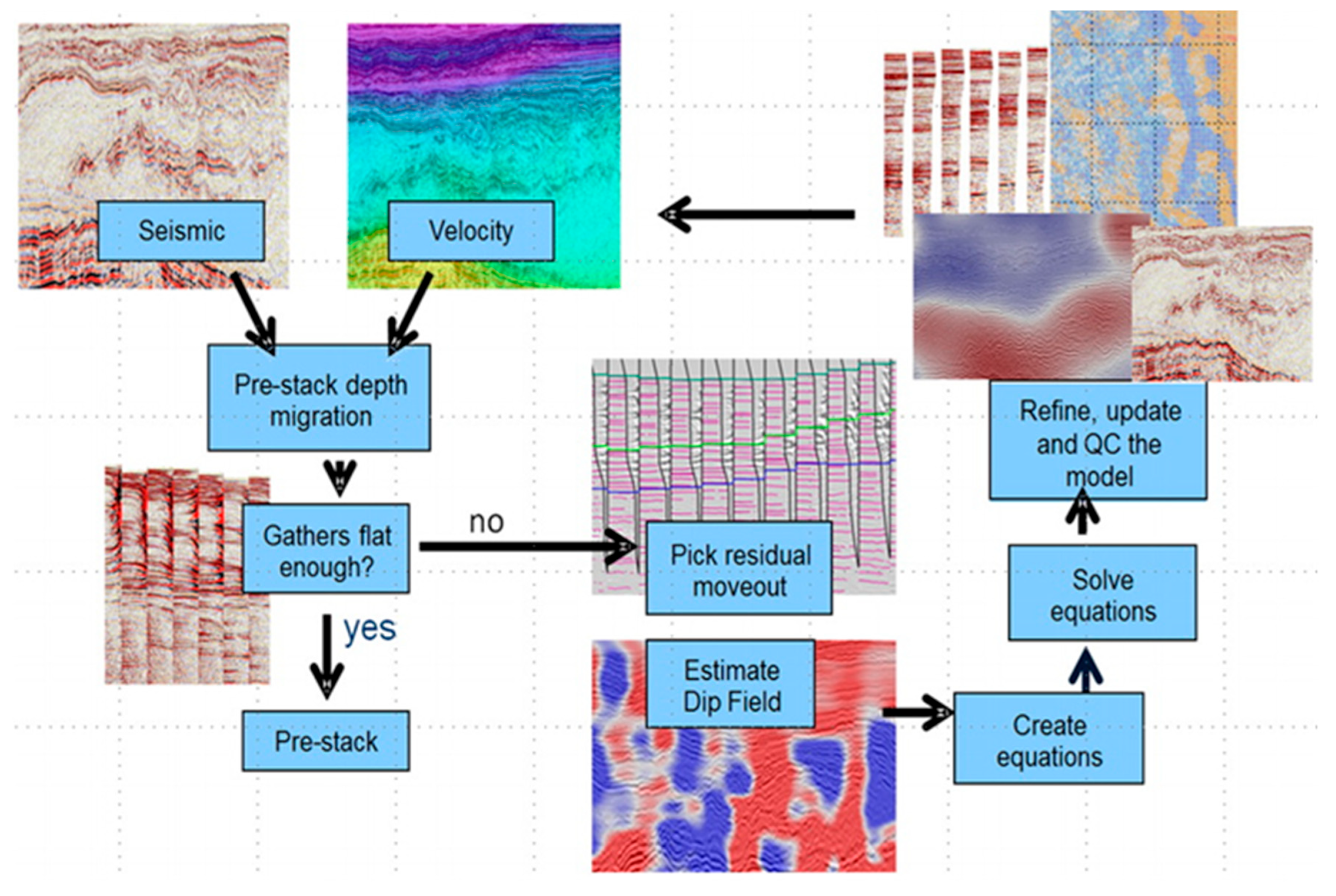
  • Three-dimensional tomographic inversion to update Vp;
  • CIP Tomography to update Vp below receivers.
The resulting velocity model is shown in Figure 13.
A generalized transform was applied to convert the time domain image into a depth domain image via the velocity model. During summation along the diffraction stack curve, different weightings are applied to the different traces based on the migration dip and dip aperture. The depth domain image is used to compare the three surveys conducted at different times. We term the first survey the baseline, the second survey Monitor 1, and the third survey Monitor 2. Figure 14 shows the baseline image on the lefthand side and the Monitor 2 image on the righthand side. It is clear that the reflectors curve in a concave-up pattern after the introduction of carbon dioxide.

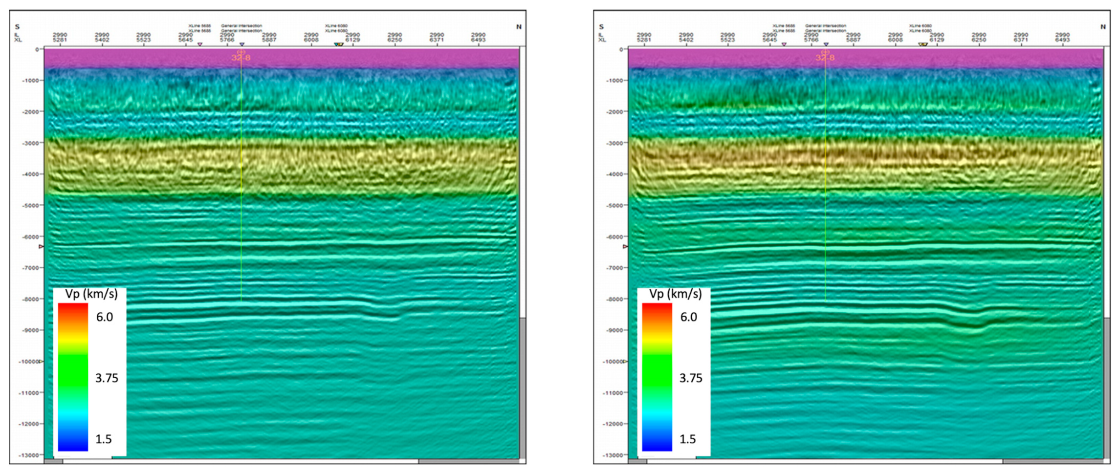
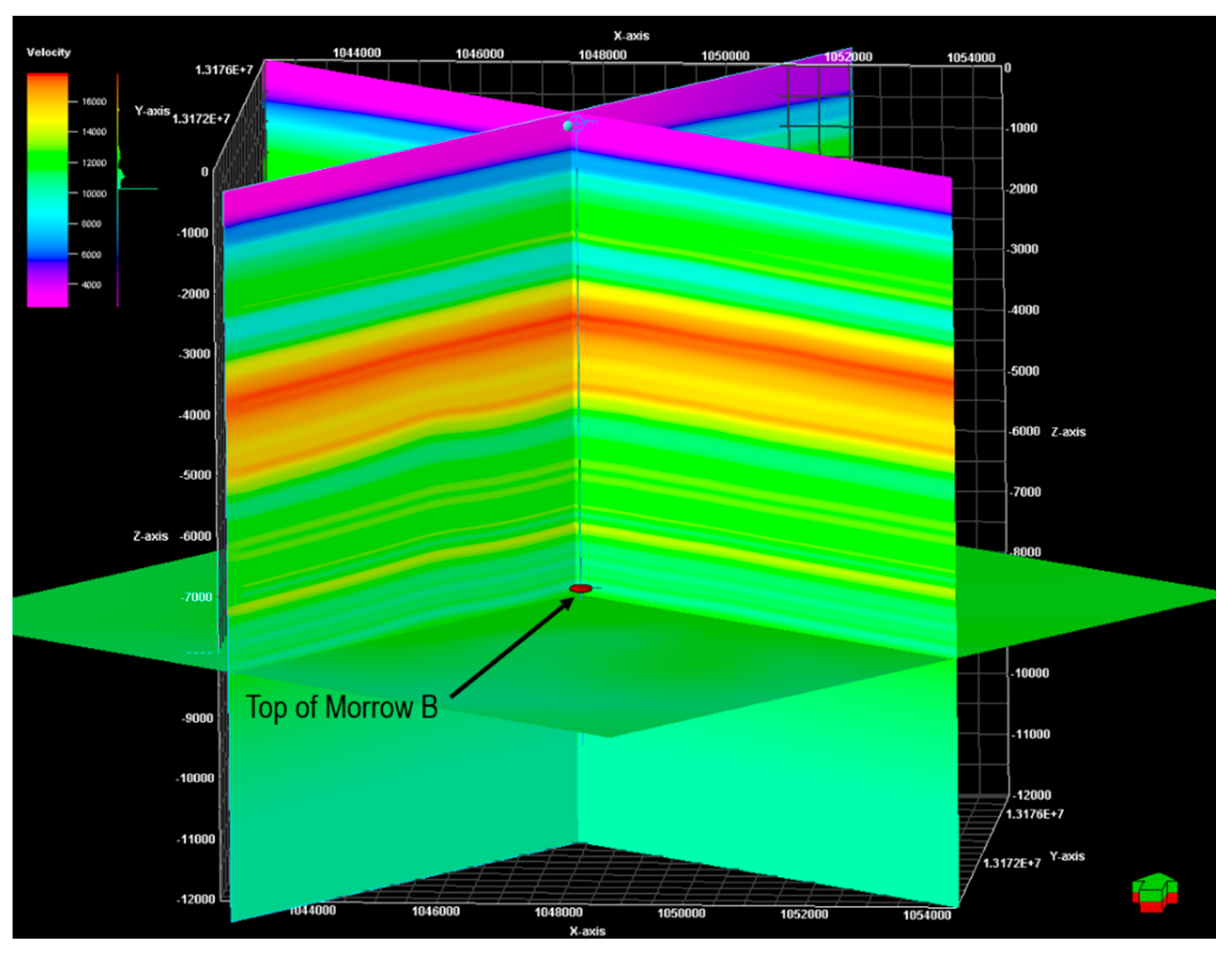
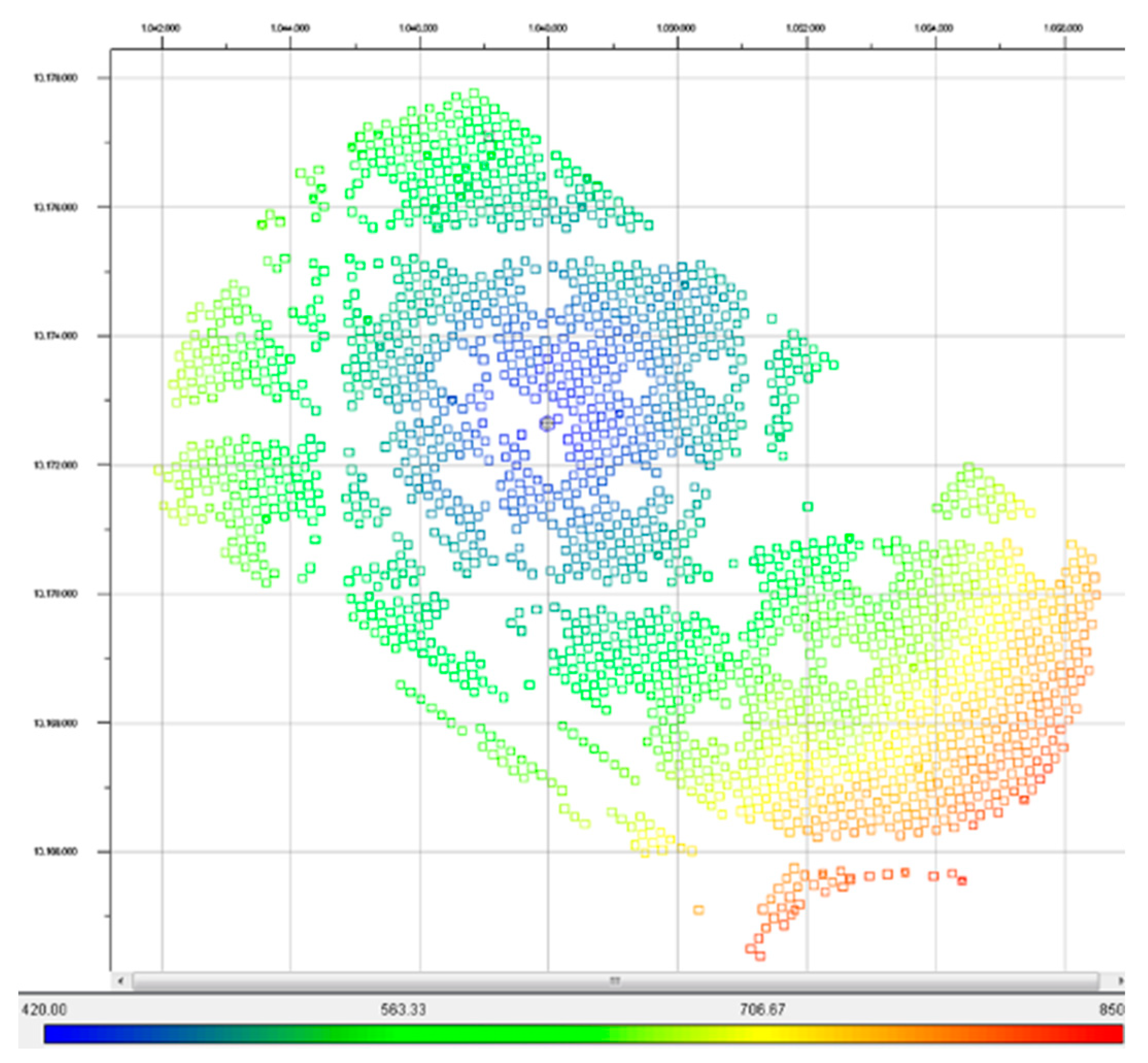
3.3. Results of the VSP

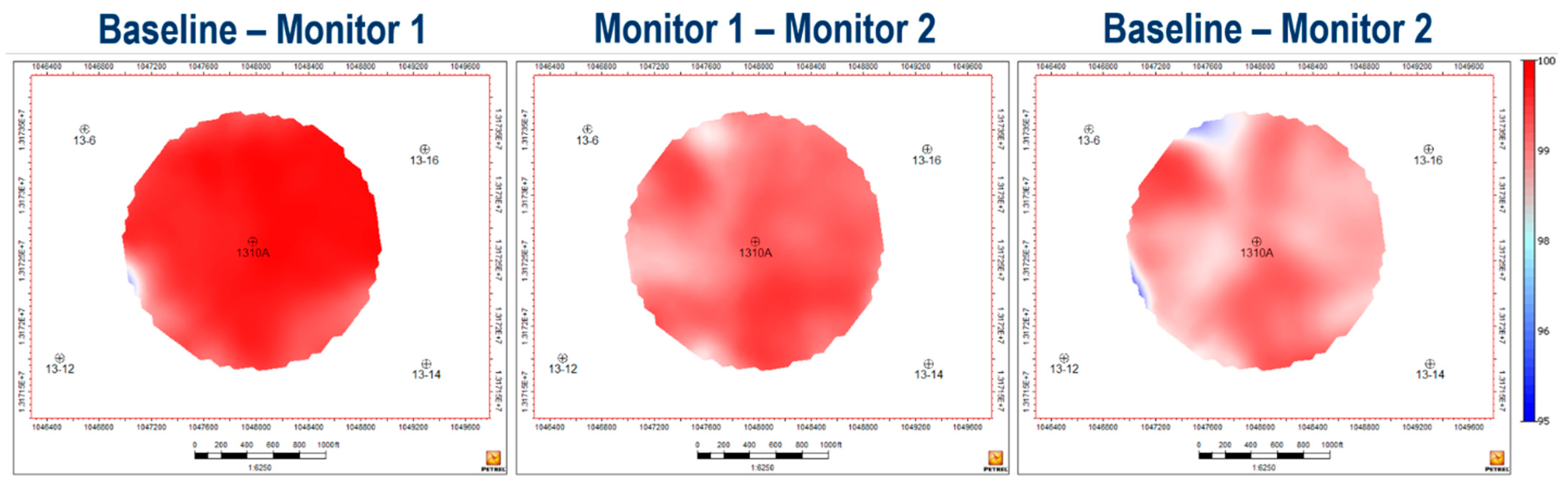
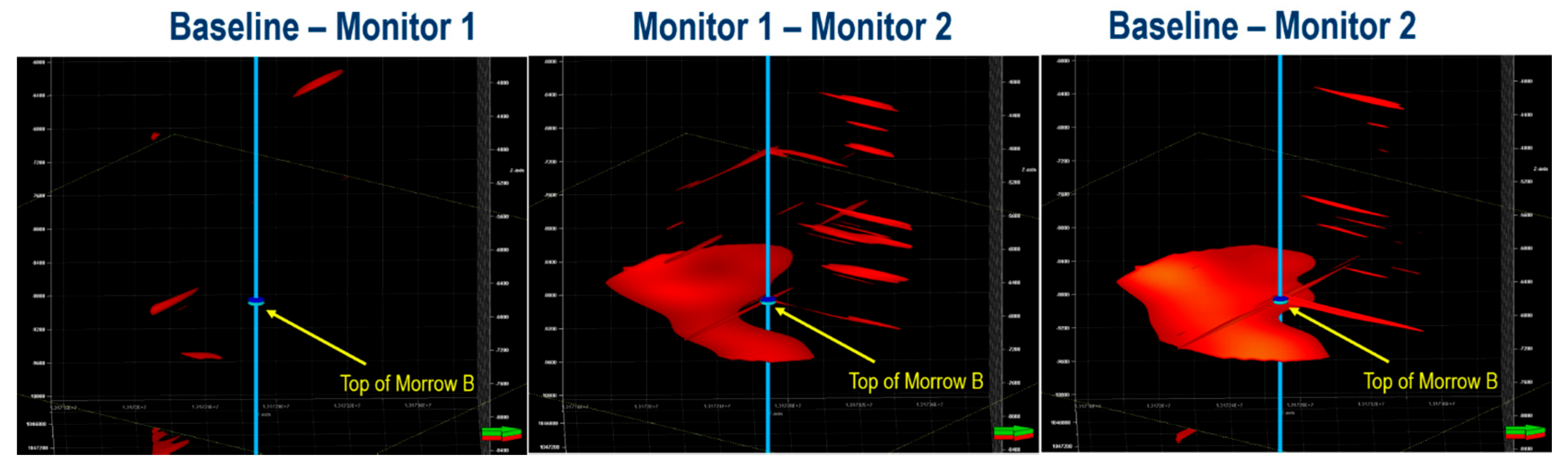
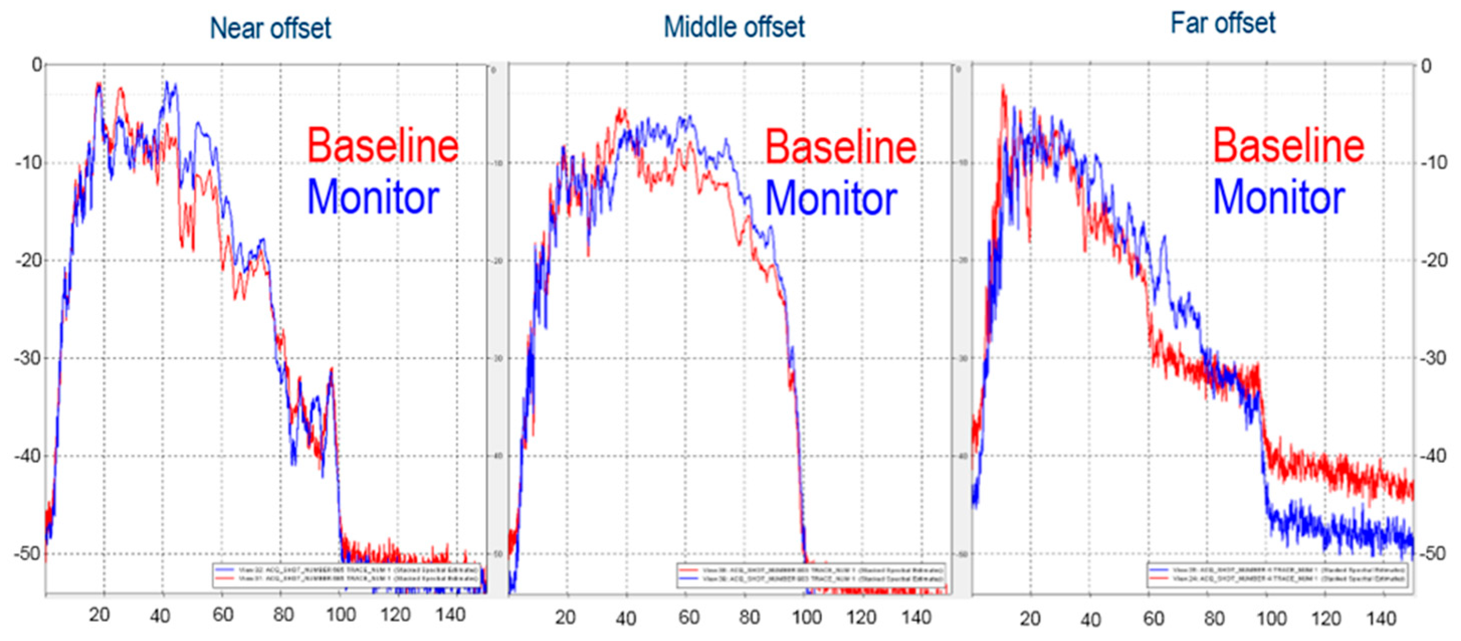
3.3.1. Timelapse Analysis

Time-lapse (4D) VSP is a geophysical measurement that is used by the oil and gas industry to monitor fluid changes within a reservoir in the vicinity of a wellbore. The technology was adopted in the Farnsworth project, as part of the monitoring program, to monitor CO2 plume development and migration in the injection reservoir (Morrow B). Changes in the fluid contents of the reservoir, replacing oil with CO2 in the case of the Farnsworth project, could potentially result in differences (time-lapse) in the seismic response between the baseline survey (no CO2 injection) and monitor surveys (post CO2 injection).
The first component of the timelapse VSP is the calculation of the cross-correlation and subsequent predictability attributes, which measure the similarity of coherence between two traces—one from the baseline and one from either monitor. Kragh and Christie [18] introduced the following predictability attribute:
P r e d i c t a b i l i t y = 100 × X c o r ( t ) 2 ( A c o r 1 ( t ) × A c o r 2 ( t )
where Xcor(t) is the cross-correlation, and Acor1 and Acor2 are the autocorrelations. Figure 15 shows the predictability in a depth range that includes the Morrow B injection zone. The change in the predictability between the baseline and Monitor 2 is substantial (rightmost panel).
The second component of timelapse VSP is the calculation of the normalized root mean squared attribute, which is also a measure of similarity between traces in separate surveys. Kragh and Christie [18] also developed the mathematical relationship for this attribute as follows:
N R M S % = 100 × ( X 1 ( t ) X 2 ( t ) ) 2 n X 1 ( t ) 2 n + X 2 ( t ) 2 n 2
where X1 and X2 are the traces and n is the number of samples in the trace. Figure 16 demonstrates the normalized root mean squared attribute for the three possible differences for the three surveys.
The radius of investigation of the timelapse VSP is limited by the edge effects that occur in processing due to migration artifacts. Therefore, we elect to use only a small area around the wellbore to display our timelapse results. In the case of the normalized root mean squared attribute, both the Monitor 1 to Monitor 2 results (Figure 16, middle panel) and the baseline to Monitor 2 results (Figure 16, rightmost panel) show a decreased similarity of waveforms, indicating that the majority of the change must have taken place during the intervening time between Monitor 1 and Monitor 2.

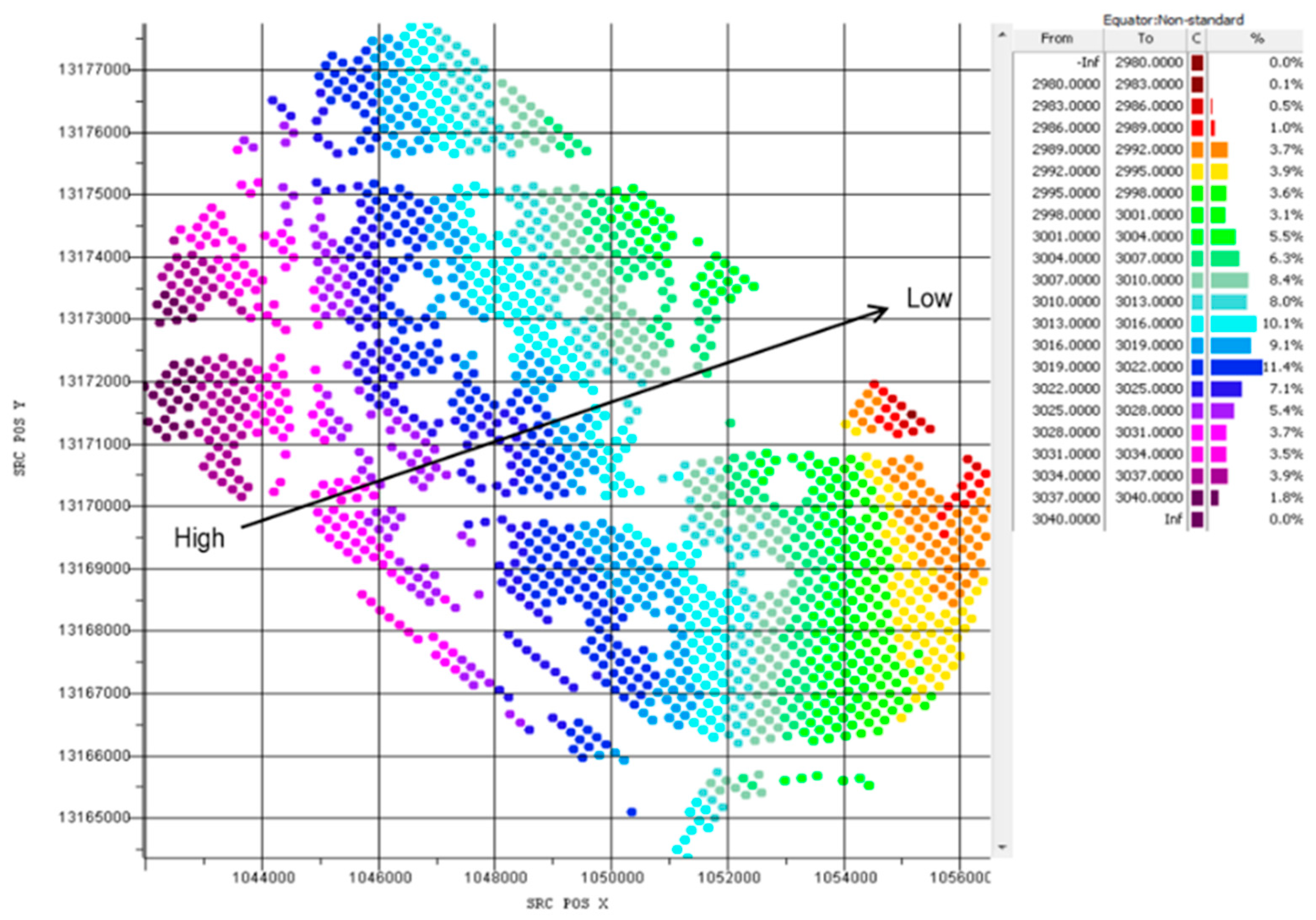
3.3.2. Displacement Field

A Non-Rigid Matching (NRM) algorithm was used to compute displacement fields in the Farnsworth project. NRM is a method which estimates the change in the two-way time (TWT) of geological features between two seismic volumes. The change in TWT may be due to a change in velocity in the surveyed area (“pull-down”), as is the case in the Farnsworth project. Variations in travel time between a baseline survey and a monitor survey indicate changes in velocity that are caused by pressure or fluid changes within the reservoir zone. The method, a trace-by-trace matching, operates on pairs of collocated traces from the two surveys. For the Farnsworth project, NRM was performed on depth-imaged cross-correlated stack volumes. The magnitude of shift, in feet, that was required to match two samples from two collocated traces was output to a 3D volume (displacement field) for analysis.
Using the NRM technique, we were able to isolate the geo-body in the volume of seismic data that corresponds to the region with depressed velocity; i.e., this is where we anticipate that the majority of the carbon dioxide is stored (Figure 17). There is a primary plume just within Morrow B, yet other secondary geo-bodies are also present.

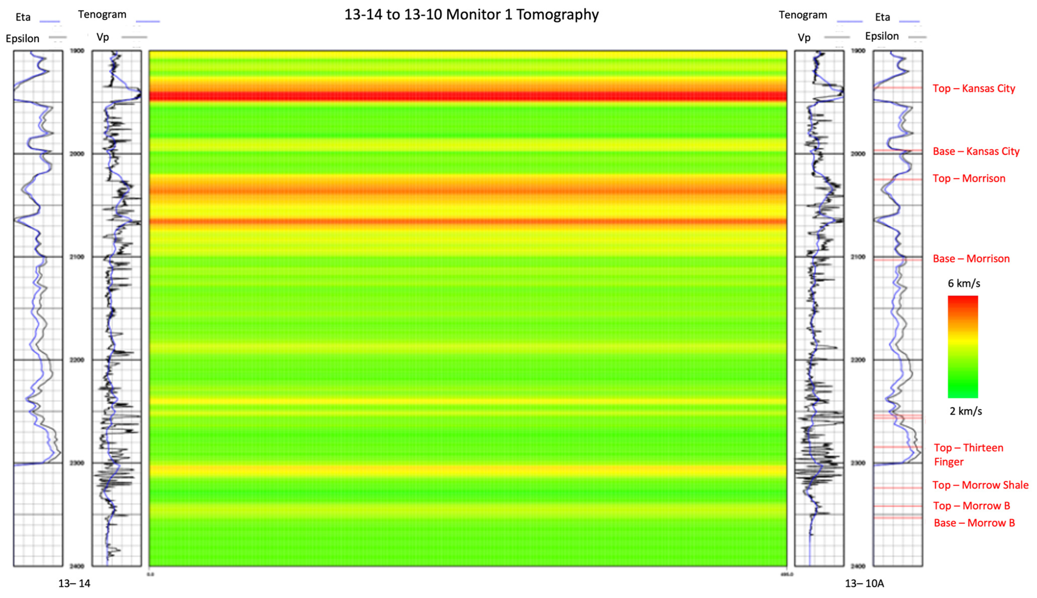
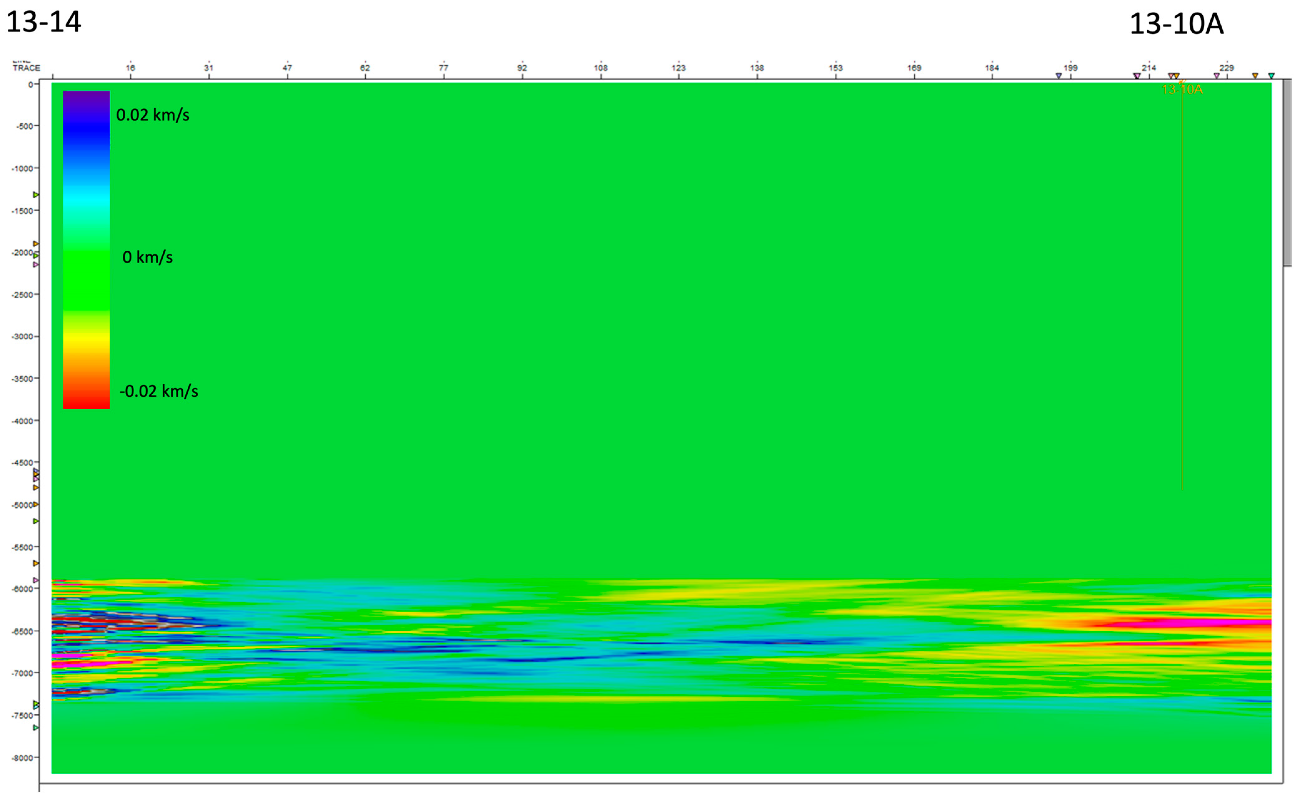
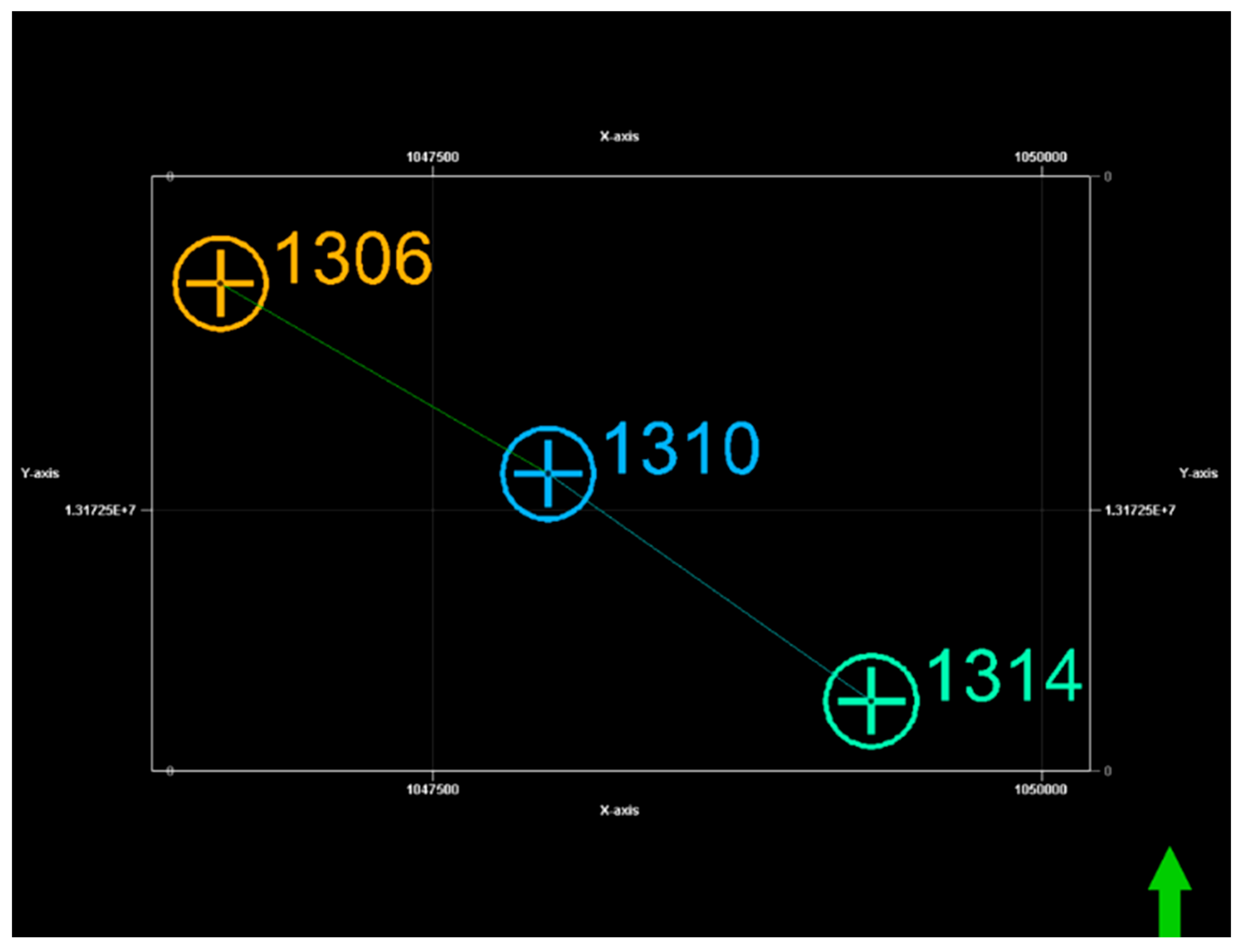
4. Cross-Well Seismic Tomography

4.1. Data Processing

Cross-well seismic tomography is another technique that is part of the larger monitoring program in the Farnsworth project. It is a geophysical method that measures the seismic signal transmitted from a source, located in one well, to a receiver array in a neighboring well. The resulting data are processed to create a reflection image or to map the acoustic velocity or other properties (velocities of P- and S-waves, for example) of the area between wells. It enables the formation between wells to be surveyed, as well as avoiding seismic signal propagation through attenuative near-surface formations. The source and receiver are usually placed near the reservoir. This method was used in the Farnsworth project in attempt to obtain a high resolution and better characterize the thin sandstone injection reservoir (Morrow B), and for the time-lapse monitoring of injected CO2 movement in the reservoir. Three baseline cross-well seismic tomography profiles were acquired in 2014 (wells 13-10A/13-06, 13-10A/13-14, and 13-14/14-01), as well as a fourth acquired in 2015 (well 32-04/32-08). Two monitor (time-lapse) profiles were acquired (wells 13-10A/13-06, 13-10A/13-14) after eight months of CO2 injection (33,070.25 tons of CO2 injected) (Figure 18).
The first step in cross-well tomography is the first arrival picking, which is performed after a number of data preparation steps including rotation to the axes of the geophones, polarity correction, and the combination of single receiver datum into array data. We used four techniques for picking and identifying the first arrivals: common receiver gathers, common source gathers, common offset (receiver depth − source depth), and common mid-depth (receiver depth + source depth)/2.

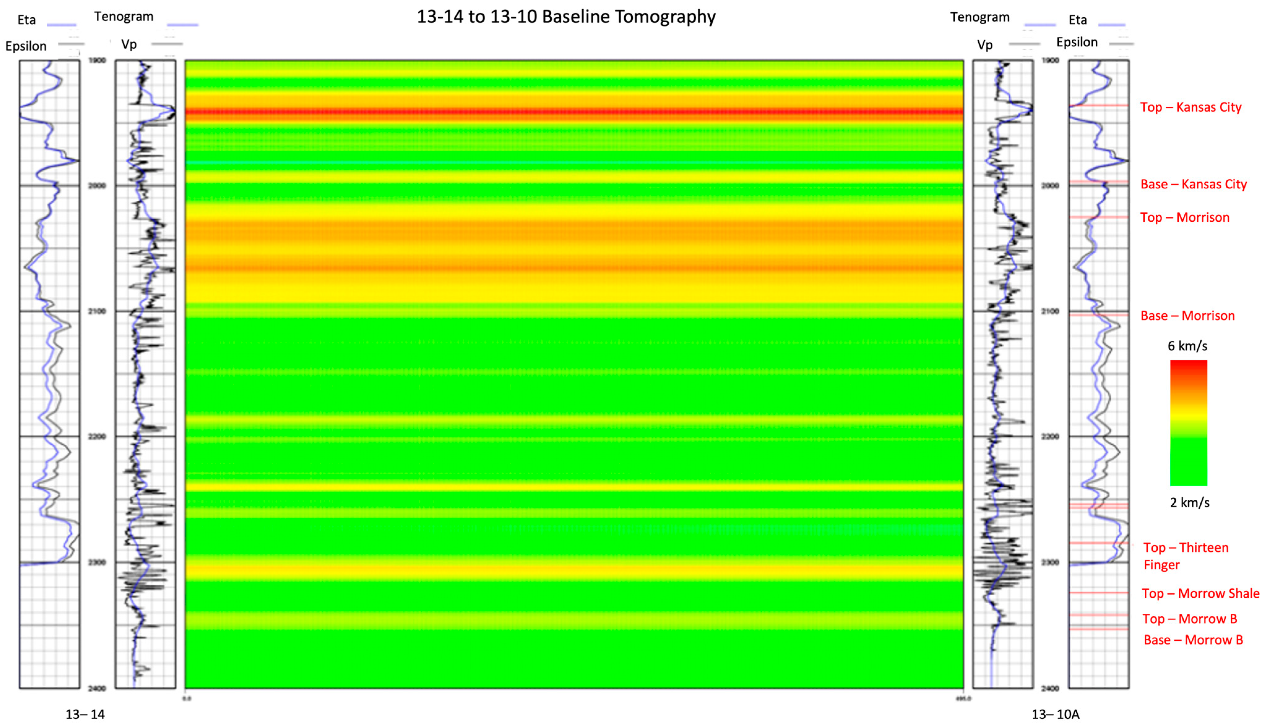
4.2. Results of Cross-Well Tomography

The results show good agreement between the cross-well seismic tomography results and available well logs (Figure 19 and Figure 20). Discerning Morrow B through seismic velocities is challenging, but achievable. However, there does not appear to be a substantial change in the velocity field between the baseline and Monitor 1, as seen in the small amplitudes of the difference between the velocities at the two times (Figure 21). All of the differences are concentrated at roughly the depth of the carbon dioxide injection, but the magnitude of the changes in velocity is very small.

5. Discussion

The three-dimensional seismic survey is an important first step to conduct the more sophisticated analyses made available by the timelapse VSP and the cross-well tomography. Not only does the three-dimensional seismic survey provide the velocity models that are necessary for the other techniques, but also it provides an enhanced understanding of the subsurface structure. Three-dimensional velocity models are also important in the location and relocation of earthquakes [19,20,21]. In addition, the processing techniques that we explored here indicate important aspects of the geology and data acquisition. For instance, the success of incorporating anisotropy into the modeling implies that the fracture networks are relatively extensive, at least in certain formations. Indeed, HTI behavior may account for some of the microseismicity that has been seen in the formations overlying Morrow B [22]. Likewise, the success of the noise attenuation algorithms may suggest that the industrial operations associated with the active oilfield have the potential to substantially interfere with the seismic processing and interpretation. Ali et al. [23] also observed potential anthropogenic sources of noise in an oilfield in Saudi Arabia. Currently, several different denoising techniques are available, such as the continuous wavelet transform and the DeepDenoiser, but they suffer from computational cost and the necessity to retrain the models for each site [24,25,26].
The timelapse VSP revealed the structure of the plume of supercritical carbon dioxide by means of the geo-body obtained from the displacement field. In the difference between the baseline profile and Monitor 1, the displacement field is minimal, but between the baseline and Monitor 2 as well as Monitor 1 and Monitor 2, there is a substantial drawdown of travel times at the location of the Morrow B formation. This geo-body is not centered on the well, which may be a result of the preferential migration of carbon dioxide or interference from other operations in the EOR field. Either explanation should be able to be confirmed by means of reservoir simulation, but having the seismic observation of the plume is invaluable for understanding the behavior of the carbon dioxide as it is sequestered. The amount of CO2 that was injected prior to Monitor 1 was 33,070.25 tons, while 76,596.64 tons were injected prior to Monitor 2. Other authors have imaged supercritical carbon dioxide plumes in the subsurface using various seismic techniques [27,28,29,30,31], but all efforts are hindered by the infrequent availability of data as well as the geometry of acquisition. The opportunity exists for new techniques that can measure the location and extent of the subsurface plume in a four-dimensional and frequent manner.
Because only cross-sections between wells can be obtained, the cross-well seismic tomography is a technique limited by the availability of such wells. In our study, the most significant changes observed in the timelapse VSP were after Monitor 2, for which there were no corresponding cross-well data acquired. In the time between the baseline and Monitor 1, more subtle changes were not able to be discerned in the cross-well seismic tomography except for a slight alteration in the velocities. Zhang et al. [32] used cross-well seismic tomography to successfully detect a carbon dioxide plume in the Ketzin Site, Germany, although they also observed several instances of decreased velocity that they attribute to processing artifacts. Böhm et al. [33] also demonstrated the feasibility of monitoring carbon dioxide plumes with cross-well seismic tomography, albeit the injection volumes are higher than those between the baseline and Monitor 1. Also, the cost of a cross-well tomography survey is appreciably lower than that of a timelapse VSP. Therefore, in certain operational conditions, cross-well seismic tomography could be significantly more illustrative than was observed here.

6. Conclusions

Three seismic methods were employed in the Farnsworth, TX, CCUS-EOR field. The first method, the three-dimensional surface seismic survey, provided a clearer understanding of the geologic structure underneath the oilfield. In addition, this method provided a three-dimensional velocity model, which is essential in the processing of the second and third methods. The second method, the timelapse VSP, revealed that most of the changes in the seismic properties occurred between Monitor 1 and Monitor 2—two surveys acquired at different times during the EOR operations. The timelapse VSP also indicated the locations of geo-bodies, which may represent the extent and position of the carbon dioxide plume in the subsurface. The primary geo-body is asymmetric with regard to the injection well, which may indicate preferential migration. While the results of the third method, the cross-well seismic tomography, aligned with well logs, they were unable to represent the changes in velocity in the interval of injection, possibly due to the lack of a second monitor survey. Cross-well seismic tomography is less expensive than the other two techniques, which, in the right circumstances, may make it more preferable.

Author Contributions

G.E.-k.: conceptualization, methodology, investigation, writing—original draft preparation. K.L.M.: writing—review and editing. All authors have read and agreed to the published version of the manuscript.

Funding

Funding for this project was provided by the U.S. Department of Energy’s National Energy Technology Laboratory through the Southwest Regional Partnership on Carbon Sequestration under Award No. DE-FC26-05NT42591.

Data Availability Statement

After completion of the project in 2024, the data will be made available to the public through the Energy Data Exchange as part of the Department of Energy (https://edx.netl.doe.gov).

Conflicts of Interest

The authors declare no conflict of interest.

References

  1. Chapman, W.L.; Brown, G.L.; Fair, D.W. The Vibroseis system; a high-frequency tool. Geophysics 1981, 46, 1657–1666. [Google Scholar] [CrossRef]
  2. Bagaini, C. Acquisition and processing of simultaneous vibroseis data. Geophys. Prospect. 2010, 58, 81–100. [Google Scholar] [CrossRef]
  3. Berkhout, A.G. Changing the mindset in seismic data acquisition. Lead. Edge 2008, 27, 924–938. [Google Scholar] [CrossRef]
  4. Lindseth, R.O. Digital Processing of Geophysical Data—A Review; Society of Exploration Geophysicists: Tulsa, OK, USA, 1968. [Google Scholar]
  5. Lucia, F.J.; Kerans, C.; Jennings, J.W., Jr. Carbonate reservoir characterization. J. Pet. Technol. 2003, 55, 70–72. [Google Scholar] [CrossRef]
  6. Xu, Y.; Chang, J.; Liu, X.; Hu, Z.; Duan, X. Modeling a Multi-Parameter Interaction of Geophysical Controls for Production Optimization in Gas Shale Systems. ACS Omega 2023, 8, 3367–3384. [Google Scholar] [CrossRef]
  7. Alvarado, V.; Manrique, E. Enhanced oil recovery: An update review. Energies 2010, 3, 1529–1575. [Google Scholar] [CrossRef]
  8. Thomas, S. Enhanced oil recovery—An overview. Oil Gas Sci. Technol. Rev. IFP 2008, 63, 9–19. [Google Scholar] [CrossRef]
  9. Ampomah, W.; Balch, R.S.; Grigg, R.B.; McPherson, B.; Will, R.A.; Lee, S.Y.; Dai, Z.; Pan, F. Co-optimization of CO2-EOR and storage processes in mature oil reservoirs. Greenh. Gases Sci. Technol. 2017, 7, 128–142. [Google Scholar] [CrossRef]
  10. Ampomah, W.; Balch, R.; Cather, M.; Rose-Coss, D.; Dai, Z.; Heath, J.; Dewers, T.; Mozley, P. Evaluation of CO2 storage mechanisms in CO2 enhanced oil recovery sites: Application to morrow sandstone reservoir. Energy Fuels 2016, 30, 8545–8555. [Google Scholar] [CrossRef]
  11. Middleton, R.S.; Bielicki, J.M. A scalable infrastructure model for carbon capture and storage: SimCCS. Energy Policy 2009, 37, 1052–1060. [Google Scholar] [CrossRef]
  12. McCormack, K.L.; Edelman, E.; Moodie, N.; McPherson, B.J.; Paulsson, B.; He, R. The Design of a Downhole Source Tomography Experiment for the Detection of CO2 Plumes in the Subsurface. In Proceedings of the 57th US Rock Mechanics/Geomechanics Symposium, Atlanta, GA, USA, 25–28 June 2023; OnePetro: Richardson, TX, USA, 2023. [Google Scholar]
  13. Balch, R.; McPherson, B. Associated Storage with Enhanced Oil Recovery: A Large-Scale Carbon Capture, Utilization, and Storage Demonstration in Farnsworth, Texas, USA. In Geophysical Monitoring for Geologic Carbon Storage; Wiley Online Library: Hoboken, NJ, USA, 2022; pp. 343–360. [Google Scholar]
  14. Balch, R.; McPherson, B. Integrating enhanced oil recovery and carbon capture and storage projects: A case study at Farnsworth field, Texas. In Proceedings of the SPE Western Regional Meeting, Anchorage, AK, USA, 23–26 May 2016; SPE: Richardson, TX, USA, 2016; p. SPE-180408. [Google Scholar]
  15. Cather, M.; Rose-Coss, D.; Gallagher, S.; Trujillo, N.; Cather, S.; Hollingworth, R.S.; Mozley, P.; Leary, R.J. Deposition, diagenesis, and sequence stratigraphy of the pennsylvanian morrowan and atokan intervals at farnsworth unit. Energies 2021, 14, 1057. [Google Scholar] [CrossRef]
  16. Egan, M.S.; Seissiger, J.; Salama, A.; El-Kaseeh, G. The influence of spatial sampling on resolution. CSEG Rec. 2010, 35, 29–33. [Google Scholar]
  17. Thomsen, L. Weak elastic anisotropy. Geophysics 1986, 51, 1954–1966. [Google Scholar] [CrossRef]
  18. Kragh, E.D.; Christie, P. Seismic repeatability, normalized rms, and predictability. Lead. Edge 2002, 21, 640–647. [Google Scholar] [CrossRef]
  19. Nugraha, A.D.; Shiddiqi, H.A.; Widiyantoro, S.; Thurber, C.H.; Pesicek, J.D.; Zhang, H.; Wiyono, S.H.; Ramdhan, M.; Wandono, W.; Irsyam, M. Hypocenter relocation along the Sunda Arc in Indonesia, using a 3D seismic-velocity model. Seismol. Res. Lett. 2018, 89, 603–612. [Google Scholar] [CrossRef]
  20. Pesicek, J.D.; Thurber, C.H.; Zhang, H.; DeShon, H.R.; Engdahl, E.R.; Widiyantoro, S. Teleseismic double-difference relocation of earthquakes along the Sumatra-Andaman subduction zone using a 3-D model. J. Geophys. Res. Solid Earth 2010, 115, B10303. [Google Scholar] [CrossRef]
  21. Lin, G.; Shearer, P.M.; Hauksson, E. Applying a three-dimensional velocity model, waveform cross correlation, and cluster analysis to locate southern California seismicity from 1981 to 2005. J. Geophys. Res. Solid Earth 2007, 112, B12309. [Google Scholar] [CrossRef]
  22. Qin, Y.; Li, J.; Huang, L.; Gao, K.; Li, D.; Chen, T.; Bratton, T.; El-Kaseeh, G.; Ampomah, W.; Ispirescu, T.; et al. Microseismic Monitoring at the Farnsworth CO2-EOR Field. Energies 2023, 16, 4177. [Google Scholar] [CrossRef]
  23. Ali, M.Y.; Barkat, B.; Berteussen, K.A.; Small, J. A low-frequency passive seismic array experiment over an onshore oil field in Abu Dhabi, United Arab Emirates. Geophysics 2013, 78, B159–B176. [Google Scholar] [CrossRef]
  24. Zhu, W.; Mousavi, S.M.; Beroza, G.C. Seismic signal denoising and decomposition using deep neural networks. IEEE Trans. Geosci. Remote Sens. 2019, 57, 9476–9488. [Google Scholar] [CrossRef]
  25. Aguiar-Conraria, L.; Soares, M.J. The Continuous Wavelet Transform: A Primer; (No. 16/2011); NIPE-Universidade do Minho: Braga, Portugal, 2011. [Google Scholar]
  26. Mousavi, S.M.; Langston, C.A.; Horton, S.P. Automatic microseismic denoising and onset detection using the synchrosqueezed continuous wavelet transform. Geophysics 2016, 81, V341–V355. [Google Scholar] [CrossRef]
  27. Ajo-Franklin, J.B.; Peterson, J.; Doetsch, J.; Daley, T.M. High-resolution characterization of a CO2 plume using crosswell seismic tomography: Cranfield, MS, USA. Int. J. Greenh. Gas Control 2013, 18, 497–509. [Google Scholar] [CrossRef]
  28. Alfi, M.; Hosseini, S.A.; Alfi, M.; Shakiba, M. Effectiveness of 4D seismic data to monitor CO2 plume in Cranfield CO2-EOR project. In Proceedings of the Carbon Management Technology Conference, Sugar Land, TX, USA, 17–19 November 2015; p. CMTC-439559. [Google Scholar]
  29. Daley, T.M.; Myer, L.R.; Peterson, J.E.; Majer, E.L.; Hoversten, G.M. Time-lapse crosswell seismic and VSP monitoring of injected CO i2n a brine aquifer. Environ. Geol. 2008, 54, 1657–1665. [Google Scholar] [CrossRef]
  30. Dodds, K.; Krahenbuhl, R.; Reitz, A.; Li, Y.; Hovorka, S. Evaluating time-lapse borehole gravity for CO2 plume detection at SECARB Cranfield. Int. J. Greenh. Gas Control 2013, 18, 421–429. [Google Scholar] [CrossRef]
  31. Freifeld, B.M.; Daley, T.M.; Hovorka, S.D.; Henninges, J.; Underschultz, J.; Sharma, S. Recent advances in well-based monitoring of CO2 sequestration. Energy Procedia 2009, 1, 2277–2284. [Google Scholar] [CrossRef]
  32. Zhang, F.; Juhlin, C.; Cosma, C.; Tryggvason, A.; Pratt, R.G. Cross-well seismic waveform tomography for monitoring CO2 injection: A case study from the Ketzin Site, Germany. Geophys. J. Int. 2012, 189, 629–646. [Google Scholar] [CrossRef]
  33. Böhm, G.; Carcione, J.M.; Gei, D.; Picotti, S.; Michelini, A. Cross-well seismic and electromagnetic tomography for CO2 detection and monitoring in a saline aquifer. J. Pet. Sci. Eng. 2015, 133, 245–257. [Google Scholar] [CrossRef]
Figure 1. Surface seismic survey area and dates of CO2 water-alternating-gas production.
Energies 16 07159 g001
Figure 2. Fold of coverage overlain on surface seismic source (east/west lines) and receiver locations (north/south lines).
Energies 16 07159 g002
Figure 3. The epsilon (left) and delta (right) Thomsen parameters for the 1925 inline in the survey. Note the high dependence on depth.
Energies 16 07159 g003
Figure 4. CIP tomography workflow.
Energies 16 07159 g004
Figure 5. (Left) Initial velocity model (overlaid on stack section) inline 2990. (Right) Final velocity model after tomography update (overlaid on stack), inline 2990.
Energies 16 07159 g005
Figure 6. Three-dimensional interval velocity model obtained from the 3D seismic survey. The horizontal section corresponds to the surface location of the Morrow B. The arrow points north with the green side indicating the upward direction.
Energies 16 07159 g006
Figure 7. Illumination map (hit count at target horizon (Morrow B)).
Energies 16 07159 g007
Figure 8. Water-alternating-gas (WAG) cycles are shown in conjunction with baseline, Monitor 1, and Monitor 2 VSP surveys.
Energies 16 07159 g008
Figure 9. Co-located sources: baseline, Monitor 1, and Monitor 2.
Energies 16 07159 g009
Figure 10. Baseline survey source elevation map.
Energies 16 07159 g010
Figure 11. Picked first arrival of baseline survey at top receiver.
Energies 16 07159 g011
Figure 12. Amplitude spectrum comparison between the baseline and Monitor 1 surveys: near, middle, and far offsets.
Energies 16 07159 g012
Figure 13. Three-dimensional velocity model, Vp. The arrow points north with the green side indicating the upward direction.
Energies 16 07159 g013
Figure 14. A comparison of the depth domain image of the baseline (lefthand side of the red vertical line) and Monitor 2 (righthand side of the red vertical line).
Energies 16 07159 g014
Figure 15. Predictability for the three differences between a 7600- to 8100-feet depth (this includes Morrow B).
Energies 16 07159 g015
Figure 16. The normalized root mean squared attribute at a depth range of 7600 to 8100 feet, which includes Morrow B.
Energies 16 07159 g016
Figure 17. The displacement field that corresponds to where the TWT has been drawn down due to the temporally changing presence of supercritical carbon dioxide. The three labeled panels represent the comparison between the three VSP surveys.
Energies 16 07159 g017
Figure 18. Geometry of the three wells used in the cross-well seismic tomography surveys. The arrow points north with the green side indicating the upward direction.
Energies 16 07159 g018
Figure 19. P-wave velocity from the cross-well tomography at the baseline time compared to well logs from the 13-14 well (left) and the 13-10A well (right).
Energies 16 07159 g019
Figure 20. P-wave velocity from the cross-well tomography at the Monitor 1 time compared to well logs from the 13-14 well (left) and the 13-10A well (right).
Energies 16 07159 g020
Figure 21. P-wave velocity difference from the cross-well tomography at the Monitor 1 time compared to the baseline. The 13-14 well is to the left and the 13-10A well is to the right.
Energies 16 07159 g021
Table 1. Surface seismic time processing workflow.
Processing SequenceDescription
Geometry UpdatePopulate seismic trace headers with geometry information (source and receiver coordinates and elevations)
StaticsRefraction Tomography
Noise Attenuation
-
Ground roll removal: Surface Wave Analysis, Modeling, and Inversion (SWAMI)
-
FX Coherent Noise suppression (FXCNS)
-
Anomalous Amplitude Attenuation (AAA)
Surface-Consistent Spectrally Constrained DeconvolutionApply frequency limited deconvolution
Model-Based Wavelet Processing (MBWP)Convolutional models containing components of the seismic wavelet and information about the noise in the data.
Residual StaticsCorrect for residual misalignment of traces
Anomalous Amplitude Attenuation (AAA)Shot, receiver and common mid-point (CMP) domains
RegularizationFill gaps in data before imaging
Kirchhoff Pre-Stack Anisotropic Time MigrationProduce 3D time migration stack volume
Disclaimer/Publisher’s Note: The statements, opinions and data contained in all publications are solely those of the individual author(s) and contributor(s) and not of MDPI and/or the editor(s). MDPI and/or the editor(s) disclaim responsibility for any injury to people or property resulting from any ideas, methods, instructions or products referred to in the content.

