Probabilistic Evaluation of Geomechanical Risks in CO₂ Storage: An Exploration of Caprock Integrity Metrics Using a Multilaminate Model

Abstract

The probabilistic uncertainty assessment of geomechanical risk—specifically, caprock failure—attributable to CO₂ injection, as presented in a simplified hypothetical geological model, was the focus of this study. Our approach amalgamates the implementation of a multilaminate model, the creation of a response surface model in conjunction with the Box–Behnken sampling design, the execution of associated numerical modeling experiments, and the utilization of Monte Carlo simulations. Probability distributions to encapsulate the inherent variability (elastic and mechanical properties of the caprock and reservoir) and uncertainty in prediction estimates (vertical displacement, total strain, and F value) were employed. Our findings reveal that the Young modulus of the caprock is a key factor controlling equivalent total strain but is insufficient as a stand-alone indicator of caprock integrity. It is confirmed that the caprock can accommodate significant deformation without failure, if it possesses a low Young’s modulus and high mechanical strength properties, such as the friction angle and uniaxial compressive strength. Similarly, vertical displacement was found to be an unreliable indicator for caprock integrity, as caprock failure can occur across a broad spectrum of vertical displacements, particularly when both the Young modulus and mechanical strength properties have wide ranges. This study introduces the F value as the most dependable indicator for caprock failure, although it is a theoretical attribute (the shortest distance between the Mohr circle and the nearest failure envelope used to measure the sensitivity to failure) and not physically measurable in the field. Deviatoric stress levels were found to vary based on stress regimes, with the maximum levels observed under extensive and compressive stress regimes. In conjunction with the use of the response surface method, this study demonstrates the efficacy of the multilaminate framework and the Mohr–Coulomb constitutive model in providing a simplified, yet effective, probabilistic model of the mechanical behavior of caprock failure, reducing mathematical and computational complexities.

1. Introduction

Anthropogenic CO₂ emissions are strongly linked to global warming [1,2,3]. In order to mitigate this issue, geologic CO₂ storage in deep subsurface environments has been identified as a viable solution [4,5,6]. Subsurface reservoirs, such as depleted petroleum reservoirs, saline aquifers, unminable coal seams, and basalt formations, have the potential to securely store large quantities of anthropogenic CO₂ for hundreds of years [7,8,9]. However, the storage of CO₂ in these formations can result in increased pore pressures and altered stresses, which may lead to undesirable consequences such as induced seismicity and damage to the integrity of the overlying caprock [10,11,12]. These impacts can compromise the sealing capacity of the formation and should be carefully considered when evaluating the feasibility of geologic CO₂ storage.

During the injection of CO₂, an increase in pore pressure and a reduction in temperature may induce geomechanical deformation in both the reservoir and surrounding rocks. The induced mechanical responses vary with time and space [13,14]. In a reservoir, the mechanical response depends on pore pressure, temperature, and stress changes [10,15]. In the caprock, overburden, or areas far beyond the injection site, the mechanical response is primarily related to stress changes [10,16]. At the beginning of injection, the increase in pore pressure is relatively small, and the mechanical responses of the rock mass may be reversible or elastic. With increasing injection pressure due to continuous CO₂ injection, irreversible mechanical changes, such as plasticity or damage, may occur. If the pore pressure is sufficiently high, rock mass failure may occur. Modes of failure include shear or tension of intact rock and the reactivation of existing faults and fractures through shear and dilation [13,16]. The reactivation of large faults and fracture corridors might induce significant seismic events. In geomechanical aspects, changes in stresses and strains, ground surface deformations, and potential hazards such as the initiation and propagation of new caprock fractures or the opening and slippage of pre-existing faults and fractures are important considerations for large-scale and long-term CO₂ storage [16]. Therefore, it is crucial to assess the geomechanical risks and stability before commencing CO₂ injection operations [15].

However, owing to the inherent uncertainty in the deep subsurface environment, the accurate prediction of geomechanical impacts is a challenging task due to the unavoidable uncertainties in the outcomes. To quantify this uncertainty, the Monte Carlo-based method has been conventionally employed for estimating a system’s output response, such as the probability density function, based on known or inferred statistical distributions of input parameters [17,18]. Although the Monte Carlo simulation method is relatively straightforward, it typically necessitates a considerable number of probability-weighted samplings of inputs, which in turn results in high computational costs to obtain a probability distribution for an output metric [19]. Moreover, numerical simulations of geologic CO₂ sequestration entail complex and computationally demanding multiphase processes [20]. Consequently, there is a growing need for the development of efficient and easily implementable methodologies within the probabilistic framework to better align with project objectives and regulatory requirements in a timely manner [21].

In contrast to the traditional Monte Carlo simulation method, the response surface methodology (RSM) [22] offers a more effective approach for various reservoir engineering applications, including performance prediction, sensitivity analyses, upscaling, history matching, and optimization studies [23,24,25]. RSM with a statistically linear model, operates with fewer runs at predetermined input points improving efficiency. Recent applications have extended to assessing geologic CO₂ storage [26,27,28,29,30]. For instance, Liu and Zhang [27] utilized a first-order model with a two-level Plackett–Burman design of experiment for the sensitivity analysis of upscaled aquifer models. Ghomian et al. [26] deployed a fractional factorial design for sandstone and a D-optimal design for carbonate reservoirs with RSM to investigate CO₂ flooding design parameters and storage. Wood et al. [29] applied the Box–Behnken design (BBD) to screen CO₂ flooding and storage in the Gulf Coast reservoirs based on dimensionless groups. Rohmer and Bouc [28] implemented a first-order polynomial approximation with Latin hypercube sampling for caprock failure assessment due to CO₂ storage. The RSM was applied to estimate the horizontal and vertical effective stress at the caprock and reservoir interface due to CO₂ injection, considering 20 variables including Young’s modulus, Poisson’s ratio, and porosity, among others. The authors of [28] identified the influential parameters for overpressure and caprock failure, with the initial effective stress emerging as the most significant variable. Raziperchikolaee and Mishra [30] also constructed predictive models to evaluate the poroelastic responses of carbonate and sandstone reservoir caprock systems related to CO₂ storage. They considered three poroelastic metrics as performance measures or dependent variables (horizontal and vertical total stress changes and reservoir displacement) and five independent variables for model predictors (Young’s modulus and Poisson’s ratio of reservoir and caprock and the pressure increase due to CO₂ injection).

This study delves into the variability of the caprock and reservoir’s elastic and mechanical properties, executing both sensitivity and uncertainty analyses. It aims to predict caprock failure estimates using a methodology that combines the RSM and Monte Carlo sampling. Additionally, a multilaminate model, accounting for the mechanical behavior of the potential pre-existing planes of weakness within caprock layers [31], is introduced to simulate caprock failure due to CO₂ injection. This research also focuses on the probabilistic delineation of temporal responses, such as vertical displacement, total strain, and F value, which are thoroughly discussed.

2. Geologic Settings and Numerical Simulation

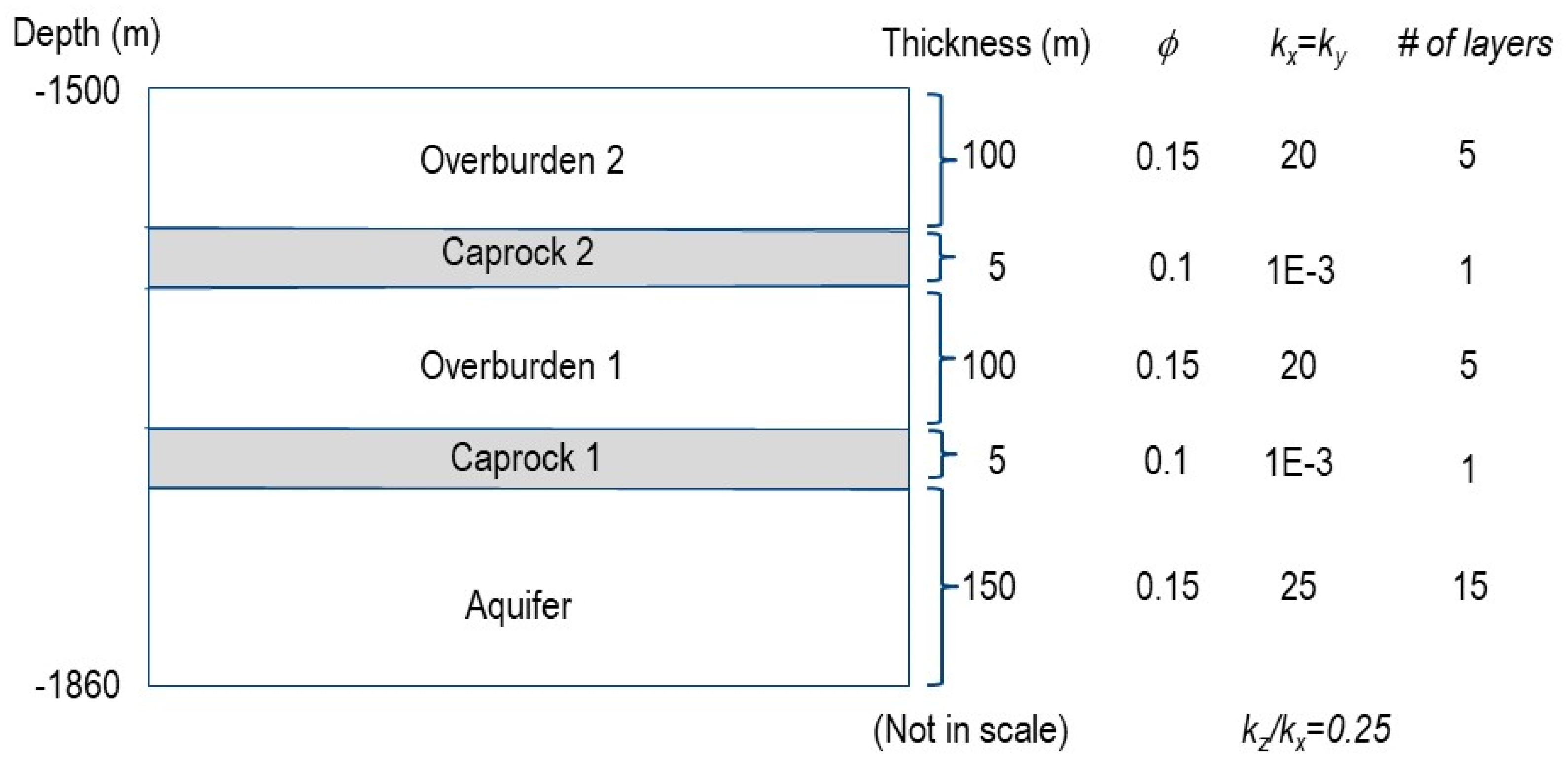
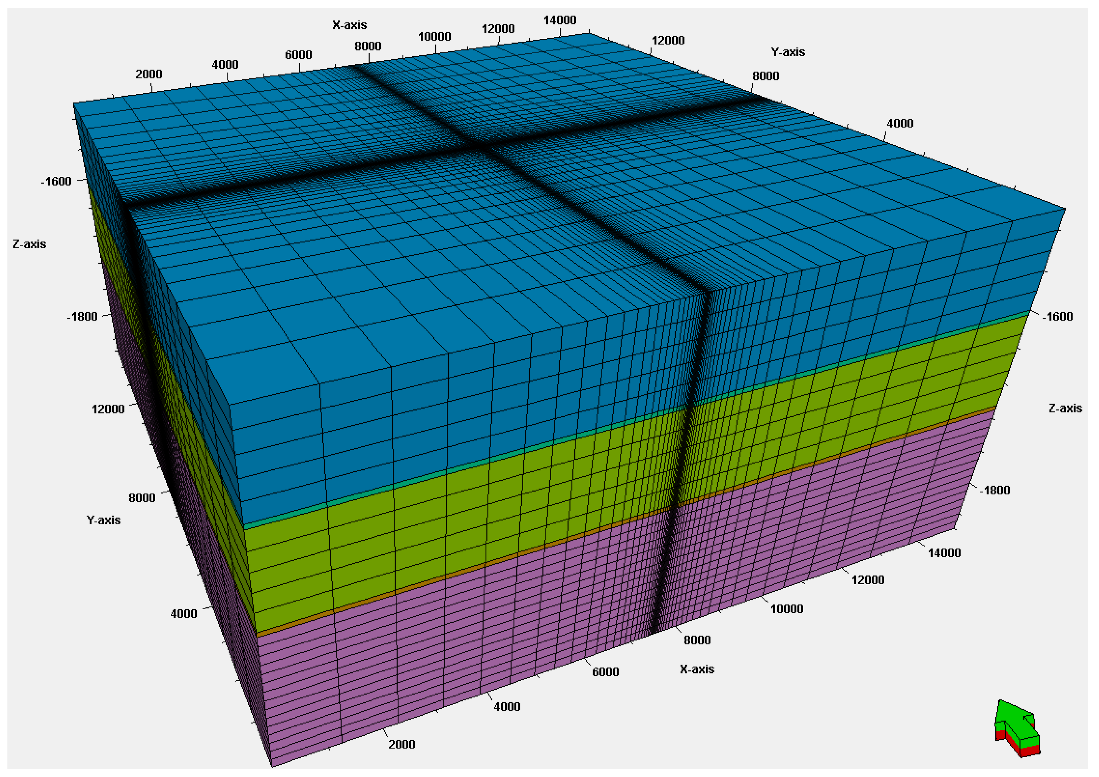
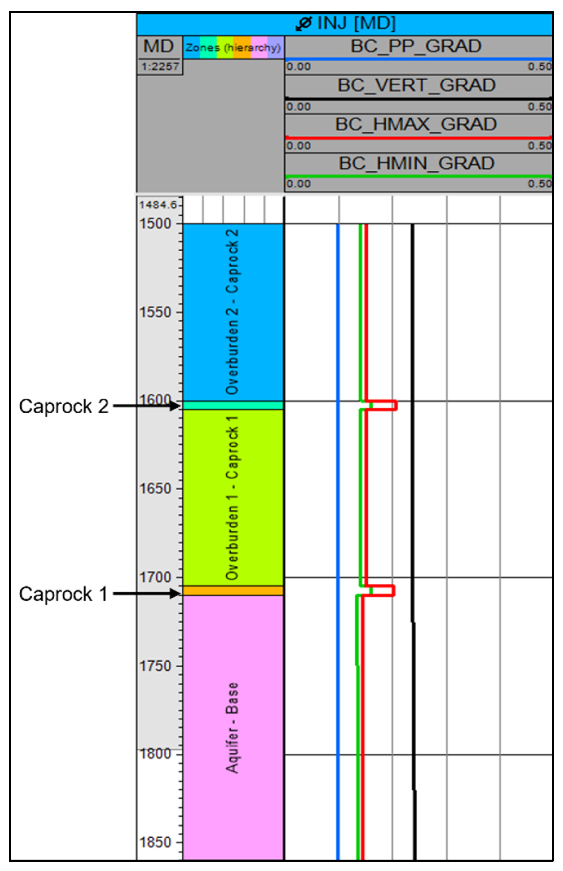
A simple layer cake 3D model was built for this study using SLB’s Petrel software platform. The model contains a sandstone aquifer body overlain by two shale caprock and two sandstone overburden intervals, with a tartan grid system centered on the single injection well. The dimensions and layering of the model are detailed in Figure 1 and Figure 2. The 3D model consists of a total of 75,843 cells (53 × 53 × 27) encompassing 15 km laterally and 360 m vertically. Applying the Tartan grid configuration, the smallest cell size in the center of the model domain is 15 m laterally and increases up to 1242.1 m in the furthest. The thickness of the storage formation and two overburden zones is 100 m each, and the caprock is 5 m thick. The vertical thickness of a cell is 5 m in the caprock, 10 m in the storage formation, and 20 m anywhere else (Figure 1). The depth to the top of the storage reservoir is 1710 m. An infinite open boundary condition was assumed with the application of a large pore volume multiplier (1 × 10⁶) to the cells along the model boundary.

Homogeneous porosity (0.15 for the aquifer and overburdens and 0.1 for the caprock) and perm (25 md for the aquifer, 20 md for the overburden, and 1 × 10⁻³ md for the caprock) were assigned. Reservoir temperature and pressure were set to be isothermal at 60 °C and hydrostatic (178.36 bar at a depth of 1820 m). Vertical anisotropy of permeability (k_z/k_x) was assumed to be 0.25.

2.1. The 3D Mechanical Earth Model

For geomechanical simulation, reservoir properties and the base geomechanical properties assigned to the 3D mechanical earth model (MEM) model are detailed in

Table 1. Reservoir and geomechanical properties assigned to the 3D MEM.

Formation	Lithology	Porosity	Perm (kx = ky)	Density (g/cc)	Young’s Modulus (Gpa)	Poisson’s Ratio	Biot’s Coefficient	UCS (bar)	Tensile Strength (bar)	Friction Angle (deg)
Overburden 2	Sandstone	0.15	20	2.35	20	0.25	1	N/A	N/A	N/A
Caprock 2	Shale	0.1	1 × 10−3	2.52	38	0.3	0.85	35	3.5	20
Overburden 1	Sandstone	0.15	20	2.35	20	0.25	1	N/A	N/A	N/A
Caprock 1	Shale	0.1	1 × 10−3	2.52	38	0.3	0.85	35	3.5	20
Aquifer	Sandstone	0.15	25	2.65	35.5	0.25	0.9	N/A	N/A	N/A
Underburden	Shale	0.1	1 × 10−3	2.65	20	0.25	1	N/A	N/A	N/A

below. The mechanical, porosity, and permeability values are based on the typical ranges of shale and sandstone properties as documented by Dobson and Houseworth [32]. Mohr–Coulomb yield criteria and associated properties were only assigned to the caprock intervals, while the linear elasticity behavior was applied to the rest of the model. The geomechanical properties were modified for the parametric and uncertainty analysis, which is described in Section 2.5.1.

2.2. Multilaminate Model

In addition to the Mohr–Coulomb constitutive model, the caprock failure mechanism was simulated with the application of a multilaminate model to account for the mechanical behavior of the potential pre-existing planes of weakness within the shale caprock layers. Typically, a discrete fracture network (DFN) is one of the more rigorous approaches to modeling the mechanical behavior of planes of weakness. In this model, individual planes in a rock mass are modeled explicitly as distinct features that deform in the normal and shear directions. This method can be used to precisely determine the explicit behavior of fractured rock masses. However, in many instances, reliable data on fracture distribution are lacking. This presents an additional significant uncertainty to caprock integrity characterization and modeling. Considering all the potential individual fractures using the DFN model is computationally impossible and practically unachievable. Probabilistic models are needed to account for the randomness in fracture geometries and distributions, and the uncertainties in the geomechanical and fluid flow properties on the response of CO₂ storage reservoirs. An alternative approach to modeling the mechanical behavior of weak planes as distinct features is using a multilaminate constitutive model. We used the multilaminate model developed by Zienkiewicz and Pande [31], which was built on the original idea by Taylor [33], who proposed that the stress–strain behavior could be specified in an independent way on different planes of the material assuming that the stress vector acting on a certain plane is the resultant of the overall stress tensor.

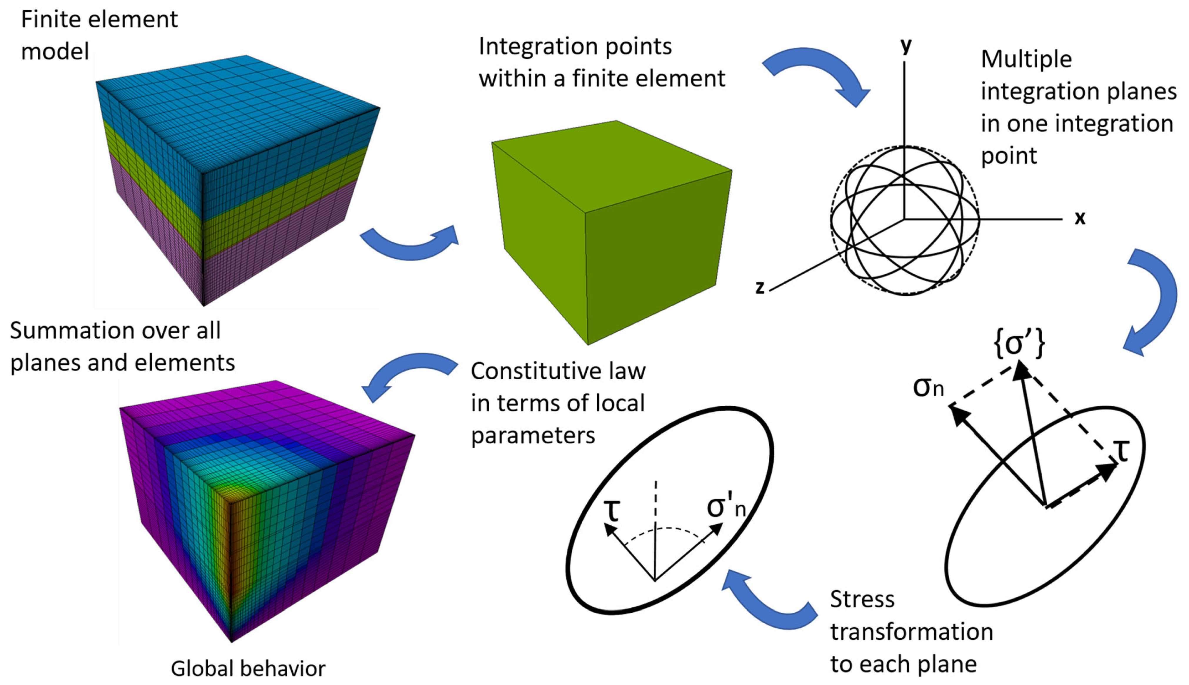
The multilaminate framework (Figure 3) establishes a simplified relationship between the microscale mechanical behavior of a material and the macroscale one. Within this framework, the global behavior of a rock can be simplified by assuming the rock body to be a combination of solid materials and a number of imaginary sliding planes oriented in space. In this work, thirteen integration points (contact planes) were assigned to each finite element cell within the caprock layers (

Table 2. The dip and orientation of the thirteen contact planes introduced into each finite element cell in the caprock formation.

Plane	Dip Angle (deg)	Dip Direction (deg)
1	0	n/a
2	45	0
3	45	45
4	45	90
5	45	135
6	45	180
7	45	225
8	45	270
9	45	315
10	90	0
11	90	45
12	90	90
13	90	135

). The microlevel stresses (normal and tangential stresses acting on a plane) were obtained by means of the projection of the macroscopic stress tensor over the plane. Yield functions were specified independently on the sampling planes; thus, during deviatoric loading, some yield surfaces were activated (those with the most favorable orientation for plastic slip), while others remained untouched. The overall plastic deformation of the rock body is the result of plastic movement along these planes under current effective stresses, calculated from the global stress tensor acting on these planes. The total deformation is the sum of the elastic deformation of solid particles and the plastic deformation of the planes.

Adopting this multilaminate framework together with the Mohr–Coulomb constitutive model allows for the inclusion of the fractured rock’s mechanical behavior along various predefined planes that are randomly oriented, in a straightforward manner without mathematical complexity.

2.3. Reservoir Flow Simulation

Given the design of the experiment specified with the BBD for four independent variables, we performed numerical modeling work for 25 cases. For the initial conditions of the model, we assumed that the model was fully saturated with water. A hydrostatic pressure (P = ρ_wgh) ranging from 148.26 bars to 181.76 bars was initially assigned according to the formation depth. Reservoir temperature was assumed to be isothermal. The assigned pressure field and temperature values maintained the injected CO₂ in its supercritical phase within the model domain.

Both the top and bottom layers of this model imposed no-flow conditions, representing the situation where the CO₂ injection formation is present under the regionally extended low-permeability caprock and above the basement rock layer. For the lateral boundaries representing the extended aquifer beyond the simulation grid, we assigned a large aquifer block to the lateral boundaries. Under these boundary conditions, the displaced brine due to the injected CO₂ was allowed to flow laterally away from the injection region, resulting in the brine displacement not exerting a downward force on the CO₂ plume and thus allowing buoyancy to act without interference.

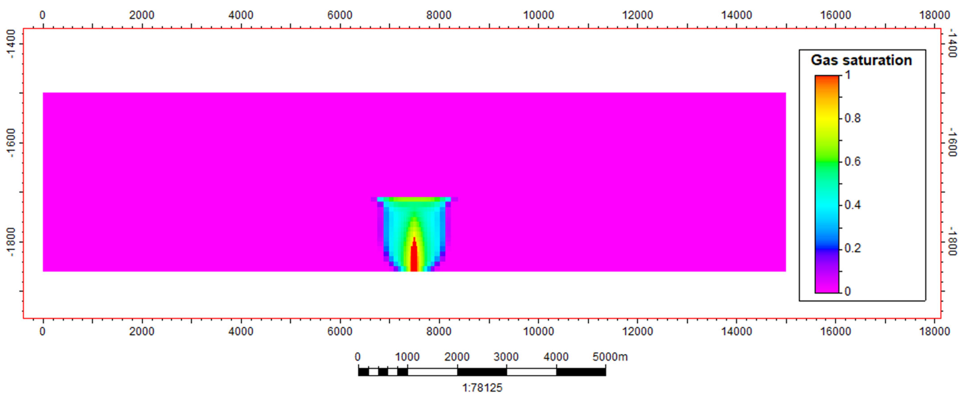
In all simulations, supercritical-phase CO₂ was injected into the aquifer continuously for 10 years with the rate of 1 MMt/year from 1 January 2017, totaling 10,000,000 metric tons. Numerical simulations were performed using the SLB ECLIPSE* reservoir simulator with the CO2STORE module [34]. We assumed that the injection well was fully perforated through the target formation. The simulated results were collected and post-processed to obtain the dependent variables for the regression and assessment. Figure 4 shows the simulated CO₂ plume distribution of base case 1 in the 8th year after the CO₂ injection activity began.

2.4. Coupled Geomechanics Simulation

Geomechanical modeling was performed using a finite element geomechanics simulator (VISAGE) [35]. Prior to the coupled simulation, stress initialization was conducted using the strain boundary condition method. Figure 5 displays the initial pore pressure and stress gradient profiles.

The resultant initialized stress model was fully coupled to the ECLIPSE reservoir simulator in a two-way manner. VISAGE uses the pressure changes from ECLIPSE at selected time steps (

Table 3. Coupled timesteps and corresponding reservoir pressure within the aquifer (injection zone).

Timestep	Max Reservoir Pressure (bars)	Max Reservoir Pressure Gradient (bar/m)	Avg Reservoir Pressure (bars)
1 January 2017	185	0.1	176
1 July 2017	208.3552	0.1125	179.9851
1 January 2018	234.9495	0.1268	183.9755
1 July 2018	234.0497	0.1264	184.2954
1 January 2019	233.1498	0.1259	184.6154
1 July 2019	232.4492	0.1255	184.6617
1 January 2020	231.7485	0.1251	184.7081
1 January 2021	230.7462	0.1246	184.7465
1 January 2023	229.0709	0.1237	184.7162
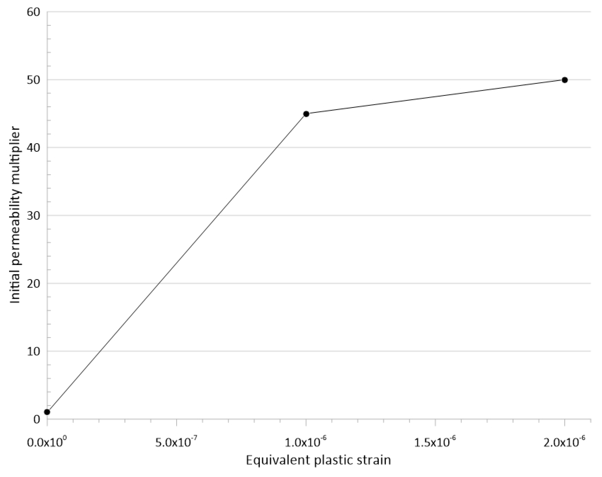
1 January 2025	227.6888	0.123	184.6551

) to perform calculations for changes in stress, deformation, and failure. To realize the two-way coupled geomechanical reservoir simulation with VISAGE and ECLIPSE, an update in permeability based on deformation was considered for the caprock intervals. In a simplified approach, the permeability is updated as a function of equivalent plastic strain, as shown in Figure 6, where an increase in equivalent plastic strain represents dilation through crack formation. Both shear and normal dilation along the fracture planes induce enhanced permeability, allowing for CO₂ migration through the caprock. In real-world projects, other permeability-updating functions based on volumetric, normal, or shear strains may be more suitable, and they will have to be calibrated with field observations to reflect realistic behavior. If available, lab measurements are helpful as well.

Base Case Results

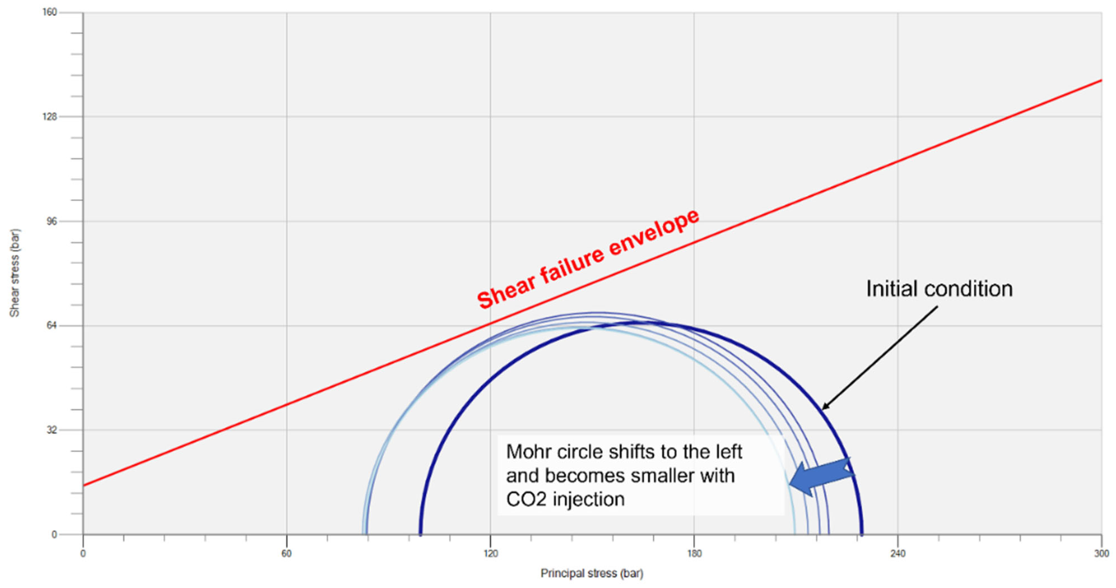
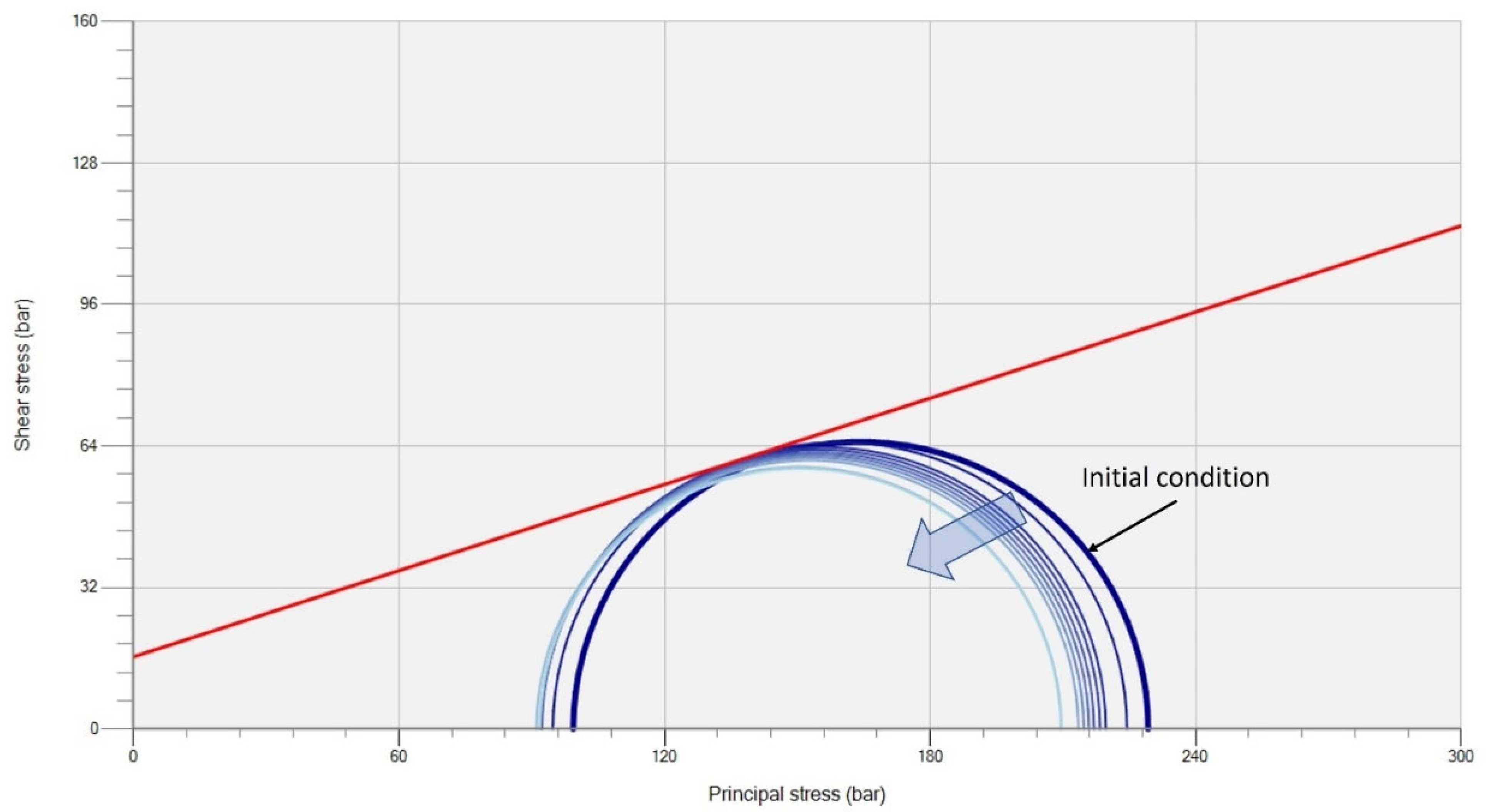
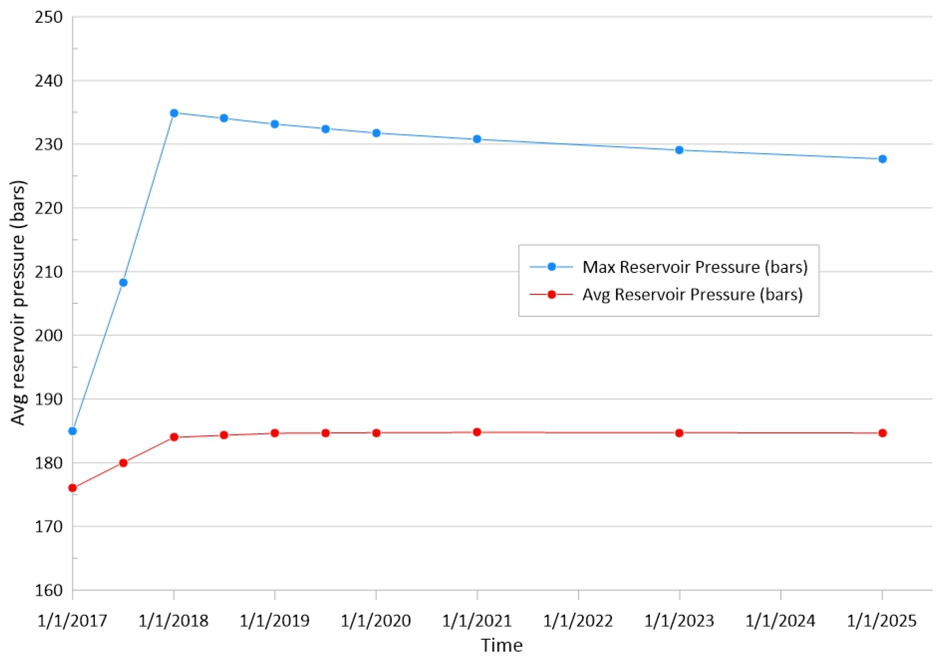
Figure 7 illustrates the plot of the Mohr circles for the cell representing Caprock 1 at the injector well. As the pore pressure increases from the CO₂ injection, the Mohr circle shifts to the left and becomes smaller. Although the Mohr circles move closer toward the shear failure envelope, no caprock integrity failure was predicted. The pressure around the injection well built up rapidly during the injection with the peak bottom hole pressure of around 230 bars (Figure 8) within the first year of injection. This analysis represents the overall rock behavior of these cells, which includes both the intact rock and multilaminate contact plane behaviors.

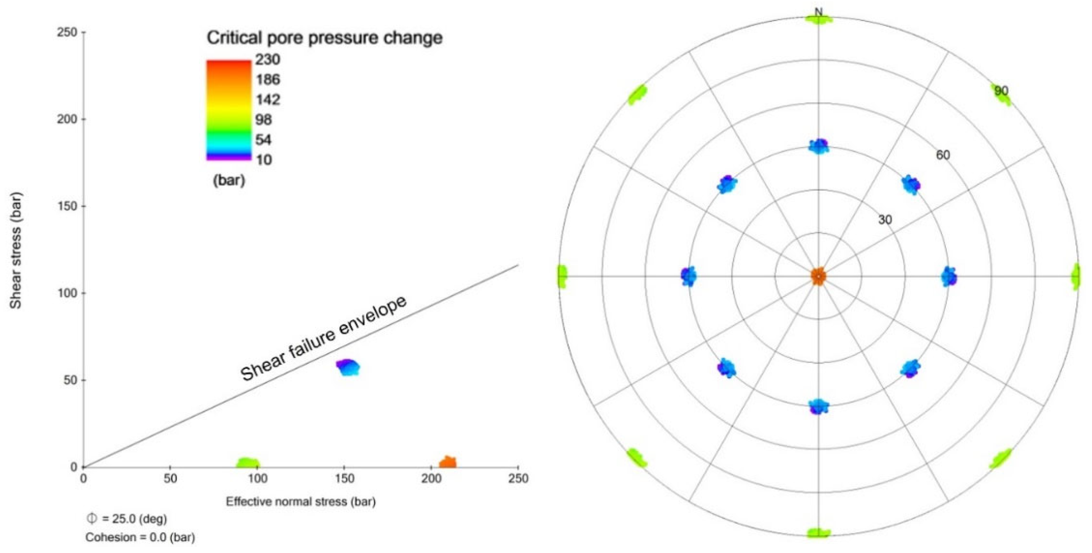
The stability of these multilaminate planes within Caprock 1 was further analyzed, and the results are presented below in Figure 9. Under the base case stress conditions, no failure was predicted throughout the CO₂ injection simulation. The planes at the 45-degree dip angle (representing Planes 3 to 9 in Table 2) are the closest to the shear failure envelope, as represented by both distance to the shear failure envelope and having the lowest pore pressure change required to induce shear failure along the plane.

2.5. Sensitivity Analysis

2.5.1. Independent Variables

For both the sensitivity and uncertainty analyses, a set of independent variables were selected, as shown in

Table 4. Independent variables along with base case and ranges considered for the simulation.

Formation	Lithology	Independent Variables		Base Case	Lower Limit	Upper Limit	Unit
Caprock (1 & 2)	Shale	Elastic properties	Young’s modulus	38	6	70	Gpa
			Poisson’s ratio	0.3	0.2	0.4	Unitless
		Mechanical strength	UCS	35	30	60	bar
			Tensile strength	3.5	3	6	bar
			Friction angle	22.5	18	27	degrees
Aquifer	Sandstone	Elastic properties	Young’s modulus	35.5	1	70	Gpa
			Poisson’s ratio	0.25	0.15	0.35	Unitless
		Reservoir properties	Porosity	0.15	0.1	0.25	Unitless
			Permeability (X = Y)	25	0.4	60	mD
All		Stress regime	R’ index	0.5 (normal stress regime)	0 (radial extensive regime)	1 (trans-tensive stress regime)	Unitless

. The independent variables relate to the elastic and mechanical properties of the caprock and aquifer formations. The base case, lower, and upper ranges of the properties are summarized in Table 4. This is not an exhaustive list of independent variables; other parameters such as formation thickness and injected CO₂ temperature were not considered for this study. The ranges of values represent typical ranges of shale and sandstone properties as documented by Dobson and Houseworth [32].

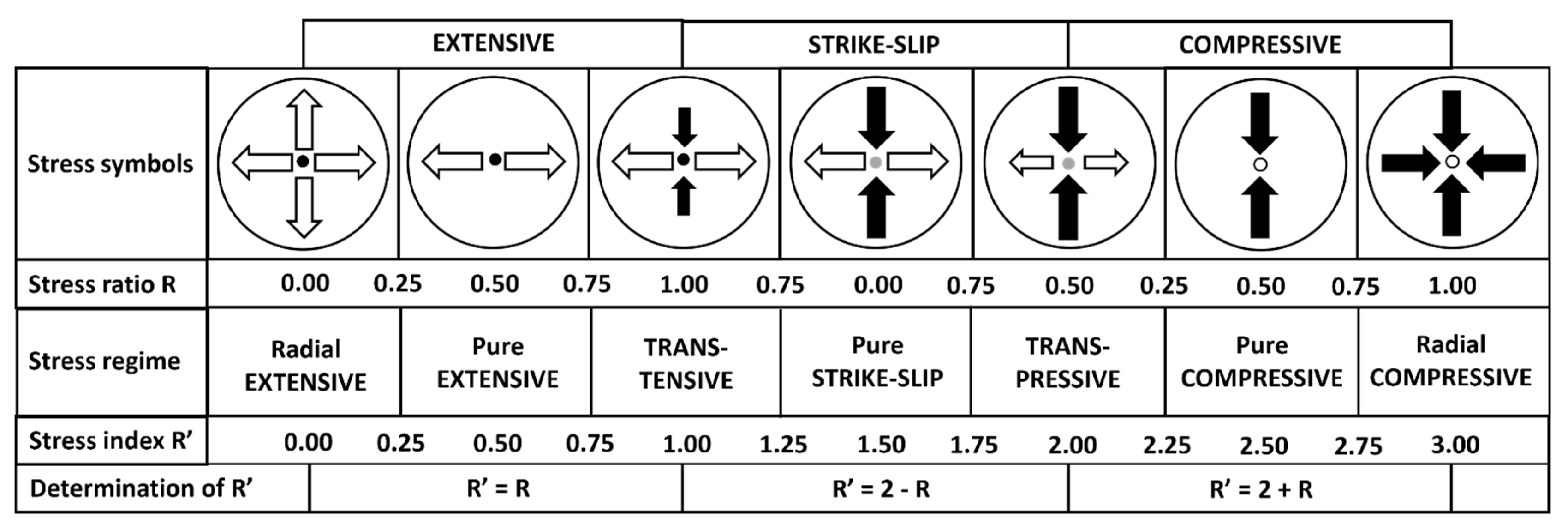
In addition to the elastic and mechanical properties, stress regime was also considered as an independent variable. The stress regime can be defined by the stress index R’ as defined by Delvaux et al. [36], which considers the stress ratio R as a function of the principal stresses expressed with Equation (1).

R = (Ꝺ₂ − Ꝺ₃)/(Ꝺ₁ − Ꝺ₃)

(1)

where Ꝺ₁ is maximum principal stress, Ꝺ₂ is intermediate principal stress, and Ꝺ₃ is minimum principal stress. An illustration of the meaning of stress regime index R’ is given in Figure 10.

2.5.2. Uncertainty Screening

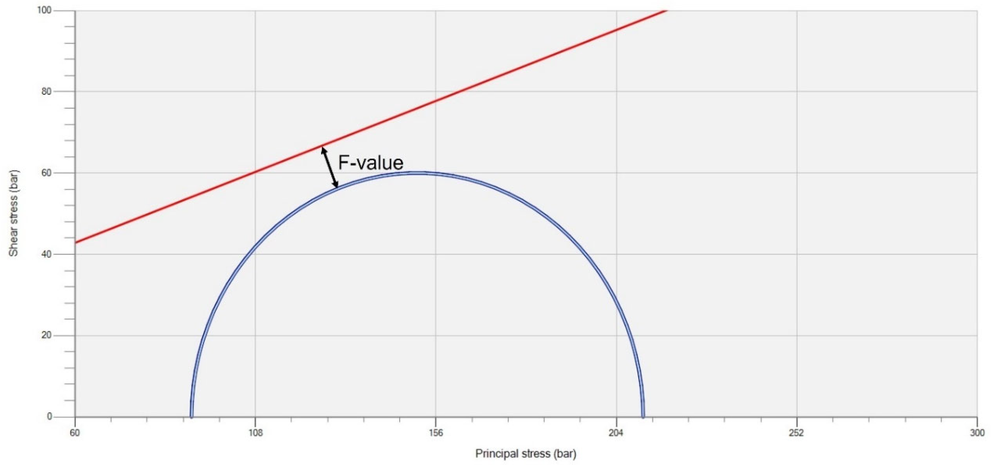
Sensitivity by one factor at a time was used to screen the independent variables. An equal-spaced sampler algorithm was used to generate a set of five equally spaced sample points between the minimum and maximum values. A numerical output, namely the F value, was used to measure the sensitivity to failure since it is considered the most meaningful proxy for caprock integrity/failure. As graphically depicted in Figure 11, the F value measures the shortest distance between the Mohr circle and the nearest failure envelope, which, in this case, is the shear failure envelope. Although this cannot be physically measured in the field, it provides a useful indicator for the sensitivity analysis as it plots the proximity to the failure envelope. A negative F value indicates a stable stress state below the failure envelope, as shown in Figure 11. In this region, the material behaves in a linear elastic manner. As the stress path moves closer to the failure envelope the F value increases and reaches zero as it intercepts the failure envelope. If the stress state moves beyond the failure envelope, the rock is in an unstable stress region, triggering shear failure and plastic deformation, which subsequently modifies the stress state to fall back onto the failure envelope. Thus, in a dynamically stable configuration, the F value will never be above zero.

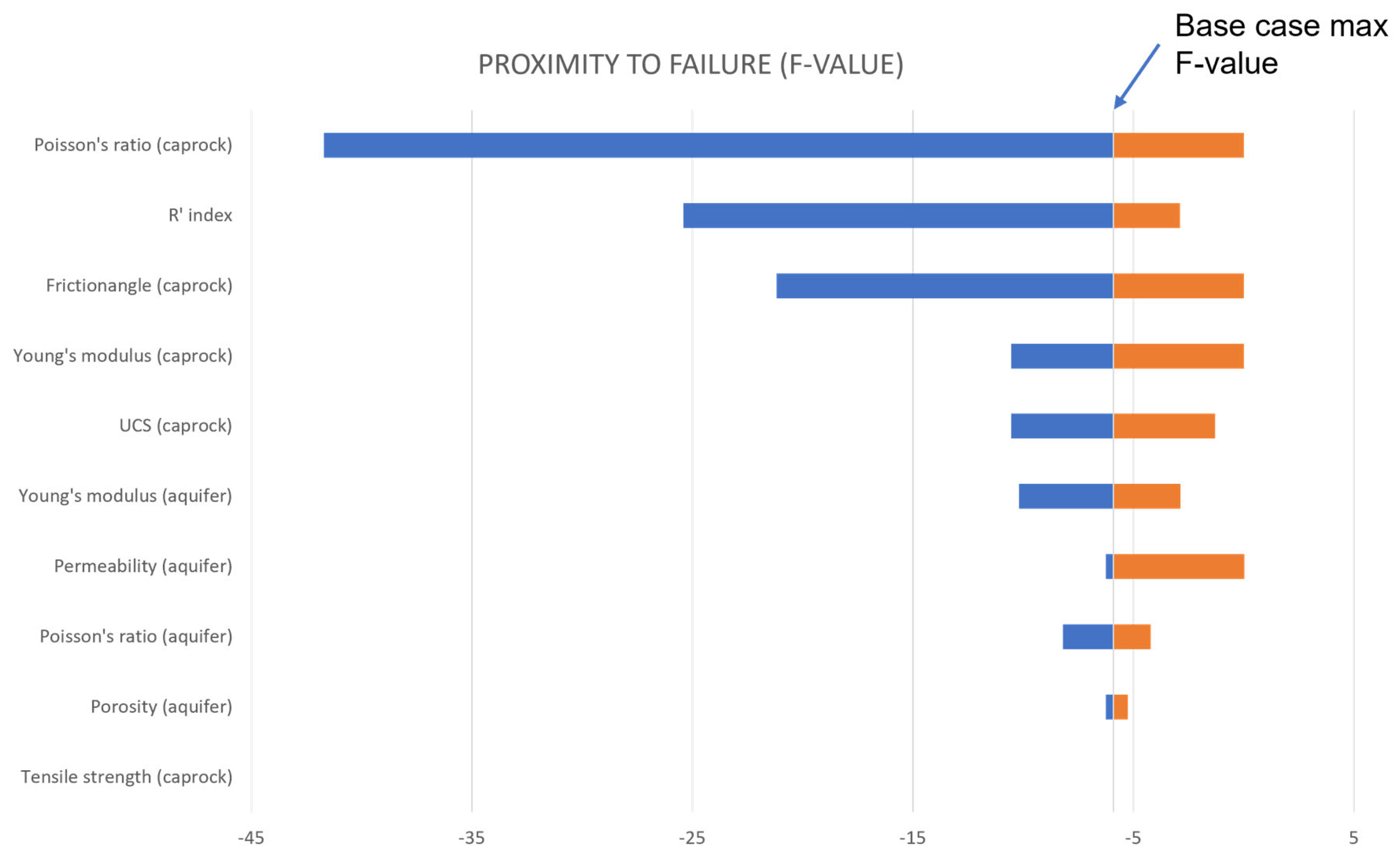
The sensitivity analysis results are summarized as a tornado chart in Figure 12, with the independent variables ranked by sensitivity based on the maximum F value (representing the closest proximity to failure). For reference, the base case scenario has a maximum F value of (−)5.91.

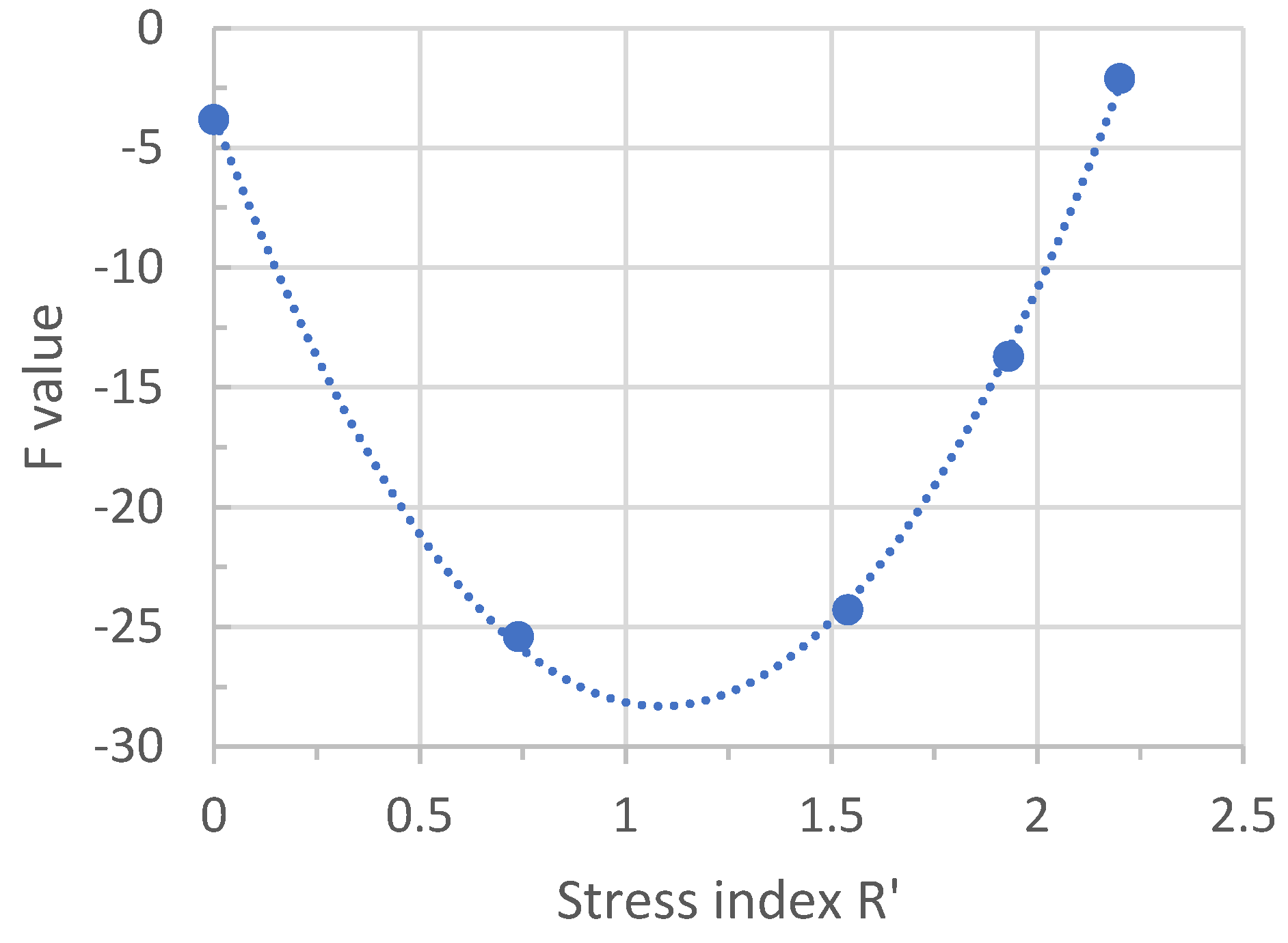
The Poisson ratio of the caprock is the most sensitive independent variable for this particular structural configuration of the model. Poisson’s ratio dictates the horizontal loading/expansion of the formation, strongly controlling the magnitude of deviatoric stress that leads to shear failure. Stress regime (R’ index) has a similar influence on deviatoric stress. However, unlike the rest of the independent variables that exhibit a linear relationship with the F value (following linear elasticity behavior), the F value variation with stress regime displays a nonlinear behavior. Rock deformation increases with deviatoric stress (difference between maximum and minimum principal stresses), resulting in a stress path toward the shear failure envelope. The F value reaches toward the maximum in extensive (R’ index = 0) and compressive stress regimes (R’ index = 2.2) (Figure 13). In these stress regimes, we find deviatoric stress to be at the maximum. The F value reaches a minimum in the strike–slip regime, where deviatoric stress is also at its minimum due to all three principal stresses being closer in magnitude.

The friction angle of the caprock controls the slope of the shear failure envelope and has a similar magnitude of sensitivity to the F value as the R’ index. In general, the elastic and mechanical strength properties of the caprock are more sensitive than those of the aquifer. The aquifer permeability has similar sensitivity as the other aquifer rock properties, while the aquifer porosity has negligible sensitivity. Since the Mohr circle evolution during injection (for these scenarios) will always intercept the shear failure envelope first, varying the tensile strength yielded the same result as the base case and showed no sensitivity.

3. Response Surface Method

Figure 14 illustrates the workflow utilized in this research. It commenced with the identification of independent variables/factors to formulate the design of the experiment (DoE) based on the Box–Behnken design (BBD), followed by numerical experiments. The dependent variables (vertical displacement, total strain, and F value) were subsequently analyzed by building a response surface model (or proxy model) for each distinct time. The stepwise regression technique was employed to exclude irrelevant factors from the regression equation, followed by the evaluation of the regression model’s performance using several goodness-of-fit measurements. Finally, Monte Carlo sampling was performed using mutually independent input parameters through the obtained response surface models for each time point. This generated temporal evolution in the cumulative distribution function (CDF) of output responses based on the given input distributions. The inter-relationship of the parameters against each dependent variable was also examined.

3.1. Design of Experiment

RSM creates a statistically linear model that is fitted to responses garnered from the DoE. The preliminary step in the DoE process involves identifying the suitable factors or design variables to be varied to predict outcomes. The principal objective of DoE techniques is to represent the sampling space as comprehensively as possible, given a finite set of laboratory or numerical experiments. Typically, the design space of factors, representing the possible values, follows linear scaling, ranging between −1 (minimum) and 1 (maximum). It is noteworthy that an inappropriate selection of the design space range in input factors could adversely affect predictability beyond the range between −1 and 1.

In this study, we employed the BBD for experimental design. The BBD is a subset of the 3k factorial design, encompassing three levels (−1, 0, and 1) for k factors. Each factor is placed at one of the three equally spaced values. The BBD has been widely used because of its economical design (less number of runs) compared with the full factorial designs [38]. Full factorial design with two levels (−1 and 1) or three levels (−1, 0, and 1) is a fully crossed design that requires 2^k and 3^k runs, respectively. As an example, for five factors, BBD requires 41 runs, whereas a three-level full factorial design demands 243 experiments. In addition, BBD incorporates interaction terms of factors and higher-order quadratic effects.

From our sensitivity analysis (Figure 12), we identified the four most sensitive independent variables: the Young modulus, Poisson ratio, friction angle of the caprock, and the R’ index. These variables were scaled to -1 and 1 for the minimum and maximum of the range, respectively.

Table 5. Independent variables used in the design of the experiment.

Independent Variables (Xi)		Low (−1)	Mid (0)	High (+1)	Statistical Distribution
X1	Caprock’s Young modulus (Gpa)	6	38	70	Normal
X2	Caprock’s Poisson ratio	0.2	0.3	0.4	Normal
X3	Caprock’s friction angle (deg)	18	22.5	27	Normal
X4	R’ index	0	0.5	1	Normal

summarizes the three levels for each. We assumed a normal distribution for all independent variables, with lower endpoint, midpoint, and upper endpoint for each. This experimental design, as outlined by the BBD, led to a total of 25 runs, and

Table 6. Design of experiment as specified using the BBD.

Case ID	Young’s Modulus (Gpa)	Poisson’s Ratio	Friction Angle (deg)	R’ Index
1	38	0.3	22.5	0.5
2	6	0.2	22.5	0.5
3	6	0.4	22.5	0.5
4	70	0.2	22.5	0.5
5	70	0.4	22.5	0.5
6	6	0.3	18	0.5
7	6	0.3	27	0.5
8	70	0.3	18	0.5
9	70	0.3	27	0.5
10	6	0.3	22.5	0
11	6	0.3	22.5	1
12	70	0.3	22.5	0
13	70	0.3	22.5	1
14	38	0.2	18	0.5
15	38	0.2	27	0.5
16	38	0.4	18	0.5
17	38	0.4	27	0.5
18	38	0.2	22.5	0
19	38	0.2	22.5	1
20	38	0.4	22.5	0
21	38	0.4	22.5	1
22	38	0.3	18	0
23	38	0.3	18	1
24	38	0.3	27	0
25	38	0.3	27	1

lists the corresponding input variables for the numerical experiments.

3.2. Response Surface Method

RSM, or regression modeling, employs mathematical and statistical techniques to establish a functional relationship between a response or dependent variable (y) and associated independent variables or factors (x₁, x₂, …, x_k). RSM typically involves creating a polynomial approximation to the responses (y) obtained with a linear regression given the input/design variables (X_i) in a selected DoE. A full second-degree RSM for k independent variables is represented in Equation (2).

$$\mathrm{y}={\mathsf{\beta }}_0+{\sum }_{\mathrm{i}=1}^{\mathrm{k}}{\mathsf{\beta }}_{\mathrm{i}}{\mathrm{X}}_{\mathrm{i}}+{\sum }_{\begin{array}{c}\mathrm{i}=1, \mathrm{j}=2\\ \mathrm{i}<\mathrm{j}\end{array}}^{\mathrm{k}}{\mathsf{\beta }}_{\mathrm{i}\mathrm{j}}{\mathrm{X}}_{\mathrm{i}}{\mathrm{X}}_{\mathrm{j}}+{\sum }_{\mathrm{i}=1}^{\mathrm{k}}{\mathsf{\beta }}_{\mathrm{i}\mathrm{i}}{\mathrm{X}}_{\mathrm{i}}^2+\mathsf{\epsilon }$$

(2)

where β_i, β_ij, and β_ii denote regression coefficients, and ε is a random error assumed to have a zero mean. For this study, k is four. Considering deterministic numerical experiments, random error due to nonrepeatability does not exist and thus is excluded. Equation (2) includes linear, two-way interactions, and quadratic terms. We determined the coefficients of the polynomial equation at each time point using the least-square method, represented in Equation (3).

$$\widehat{\mathsf{\beta }}={\left({\mathrm{X}}^{\prime }\mathrm{X}\right)}^{-1}{\mathrm{X}}^{\prime }y$$

(3)

The BBD was used for the matrix X with four factors. Only significant variables and interaction terms (at the 95% significance level) were included in the RSM after applying a stepwise regression procedure. This iterative procedure involves repeatedly modifying the model by adding or removing a predictor variable based on its statistical significance, continuing until an alteration is no longer feasible due to the stepping criteria or maximum number of steps reached.

We performed post-processing for the numerical outcomes of the equivalent total strain, vertical displacement, and F value, all of which were the dependent variables under evaluation. The equivalent total strain combines all vector components of strain into a simplified scalar measure, encompassing both elastic and plastic strains (if the material has yielded). Vertical displacement is used to quantify the degree of displacement in the vertical direction. Both these variables can be conveniently measured in the field as part of a monitoring program, utilizing equipment such as surface tiltmeters or down-hole strain gauges. The F value, as previously explained, was employed to assess sensitivity to failure. This metric is deemed a crucial indicator of caprock integrity and failure in numerical models.

3.3. Goodness-of-Fit Measurements

To quantitatively assess and validate the simulated outcomes’ fit to the observed values, we employed two measures: the mean absolute error (MAE) and the coefficient of determination (R²). The MAE is calculated using Equation (4) as follows:

$$\mathrm{M}\mathrm{A}\mathrm{E}=N^{-1}{\sum }_{i=1}^N|y_i-f_i|$$

(4)

where y_i and f_i denote observed and simulated responses, respectively, at case i. Expressed in the units of the variable, the MAE provides a direct measure of the average magnitude of errors. R² is calculated using Equation (5).

$$R^2=1-\frac{\sum _{i=1}^N{(y_i-f_i)}^2}{\sum _{i=1}^N{(y_i-\overline{y})}^2}$$

(5)

where $\overline{y}$ is the mean of the observed data. R² measures the degree of variation in the response that can be explained using the model. We initially established that models with an R² value greater than 0.9 were acceptable based on our predefined criteria. However, if the R² value did not exceed this threshold, we still considered the model acceptable, provided that the other goodness-of-fit measures indicated an acceptable tolerance level. For example, we determined the mean squared error (MSE), normalized MSE (NMSE), normalized root-mean-squared error (NRMSE), mean absolute relative error (MARE), coefficient of correlation (R), and coefficient of efficiency (COE) to further investigate whether the response model is statistically acceptable. Figure 15 shows the cross-plot of the simulated and predicted total strain, vertical displacement, and F value at t = 1 year with the goodness-of-fit measure results.

3.4. Monte Carlo Simulation through RSM

A sequence of random combinations, derived from the input distributions of the input factors, is implemented into the tailored response surface equation, thereby generating a large number of realizations. This process culminates in a probabilistic distribution function of the output variable. Our study involved executing 10,000 iterations of Monte Carlo samplings in association with the established RSM for each dependent variable and time. It is important to note that these dependent variables are statistically mutually independent. Each iteration signifies a combination of input variables sampled from the designated probability distributions, contributing to the development of a probability distribution in the result.

Figure 16 presents the series of independent probability density functions (PDFs), each obtained at specific times for the total strain, vertical displacement, and F value. The smooth transition within the PDFs was achieved through appropriate adjustments in the output interval, facilitating the interpolation of probability distribution functions from one time point to the next. As the dependent variables underwent significant changes due to caprock failure during the 1-year injection period, it was imperative to decrease the output interval during and immediately following the injection period. Consequently, the temporal evolution of the probability distribution functions was plotted for each dependent variable, providing a comprehensive final result.

4. Results of Probabilistic Risk Assessment

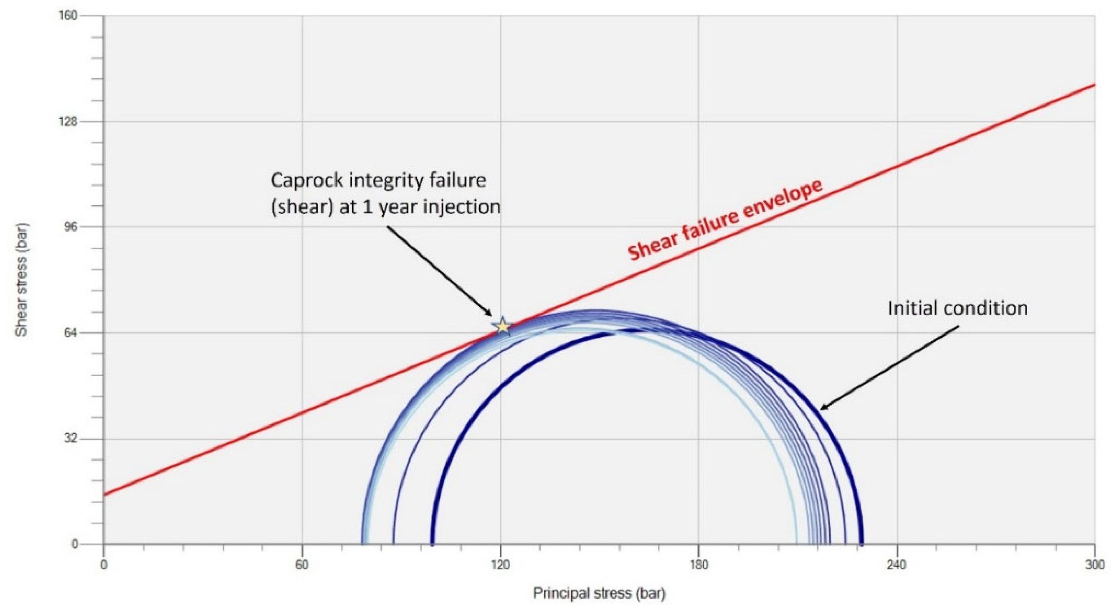
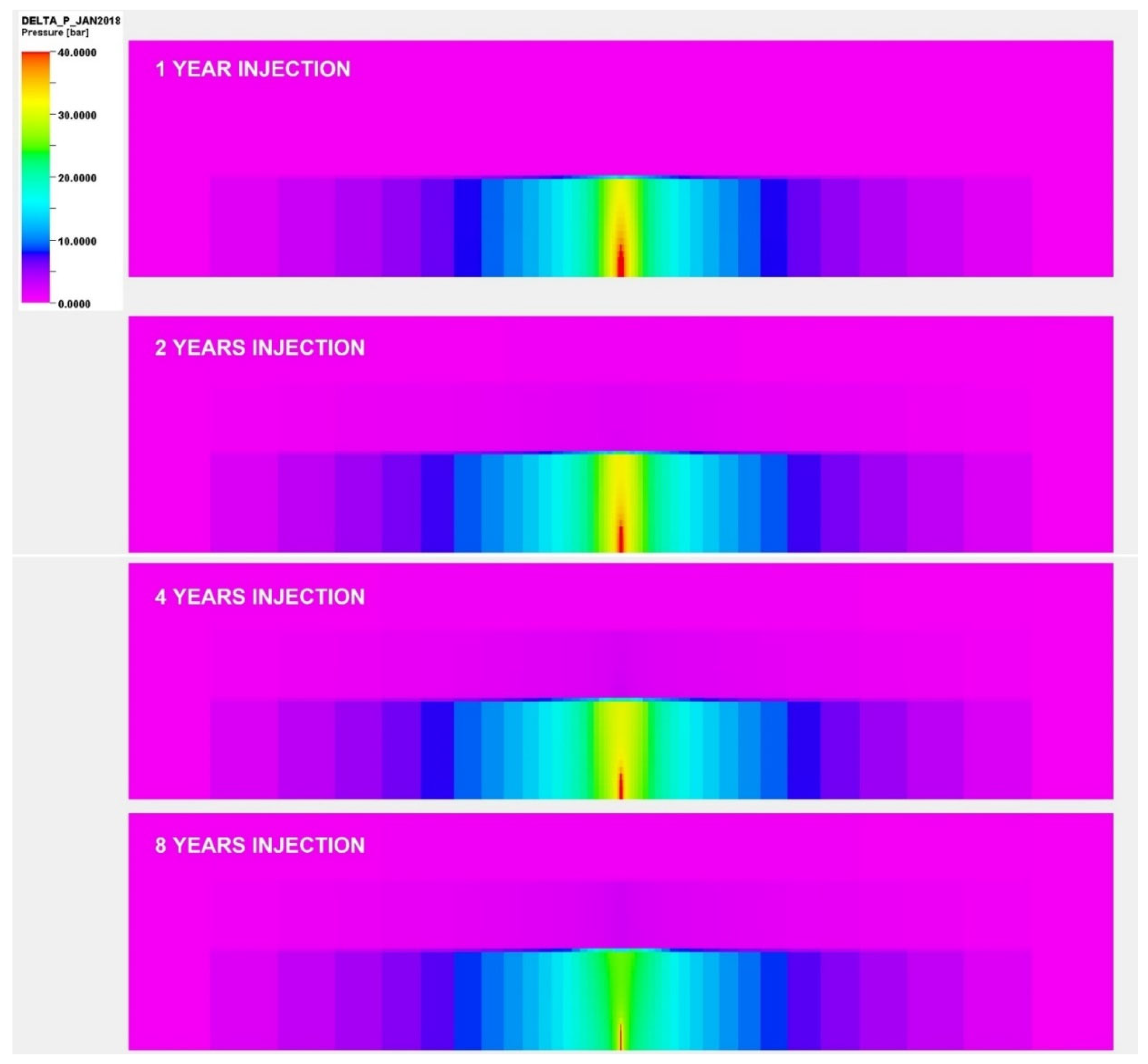
Out of the 25 cases studied, only a handful of cases resulted in caprock integrity failure. Case ID 12 is one such example, where shear failure in Caprock 1 is predicted by the end of the 1st year of injection (Figure 17). As shown in Figure 18, the pressure build-up both in the reservoir and in the caprock is most pronounced and localized at the end of the 1-year injection period, resulting in the Caprock 1 failure directly above the injection location. 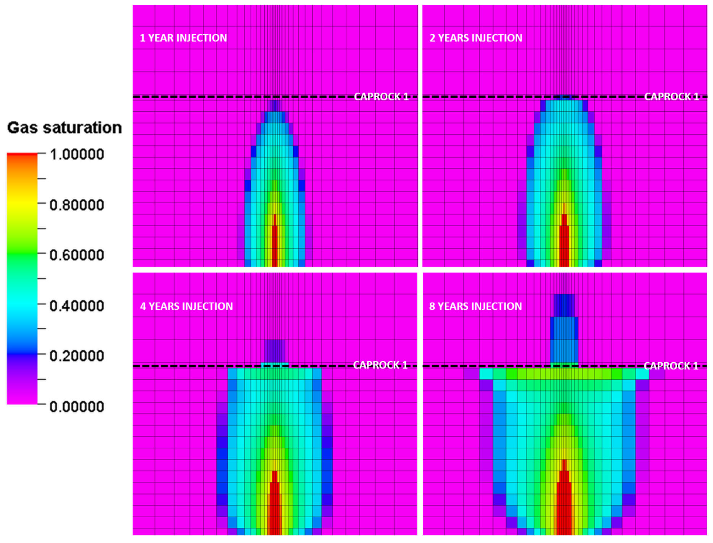As the CO₂ injection continued, the plume became more spread out and in the process diffused the pressure build-up over a larger volume, exerting less stress and associated deformation on Caprock 1. However, the shear failure in the caprock at the end of the 1-year injection period resulted in the activation of some yield surfaces (plastic movement) along the predefined planes associated with the multilaminate model. These slip planes remained active there throughout the remaining simulated injection period, creating multiple conductive pathways for the injected CO₂ to migrate through the caprock and into the overlying overburden formation, as shown in Figure 19 for the evolution of the CO₂ plume. If pressure measurements immediately above Caprock 1 were available, the cohesion values of the planes could be calibrated to match actual pressure observations to increase the robustness of the multilaminate model.

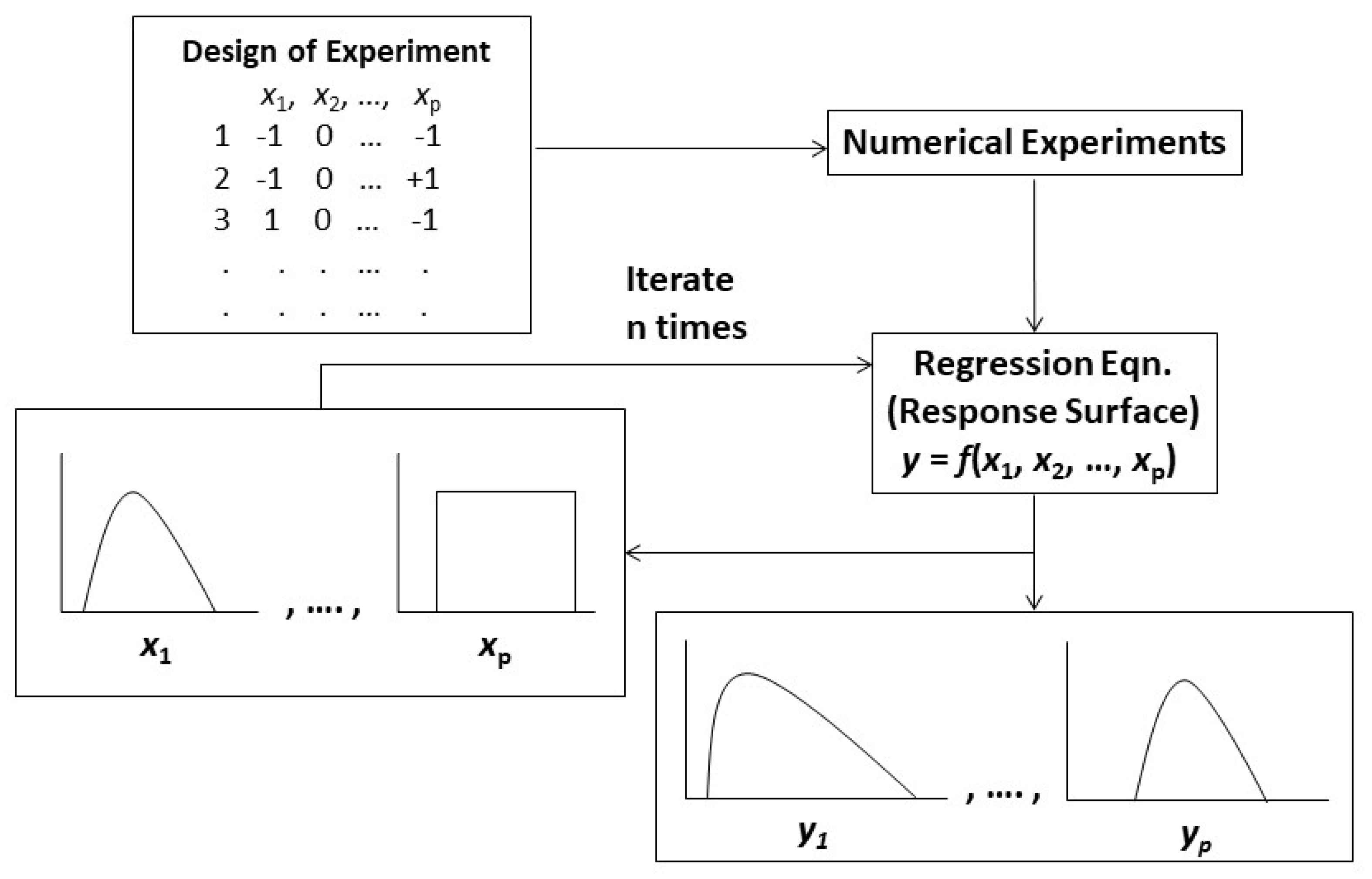
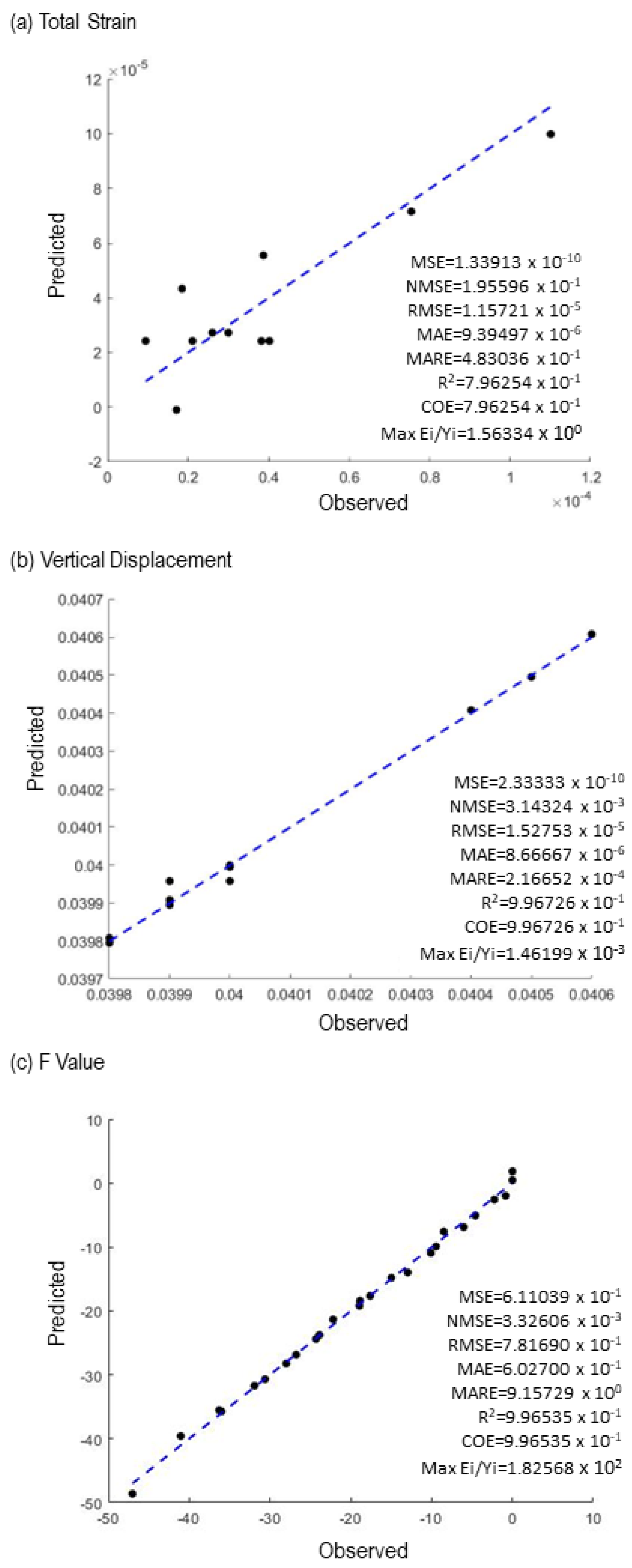
As described in the previous sections, we constructed an RSM associated with a four-factor BBD experimental design and performed the regression modeling with the stepwise regression method on the outcomes (responses) from the specified numerical runs. After building the regression models for each dependent variable at each time, we performed the Monte Carlo simulation with the fitted regression equation at each time. The post-processing of the results includes the collection of the dependent variables (y = vertical displacement, total strain, and F value) for the assessment of geomechanical risk analysis.

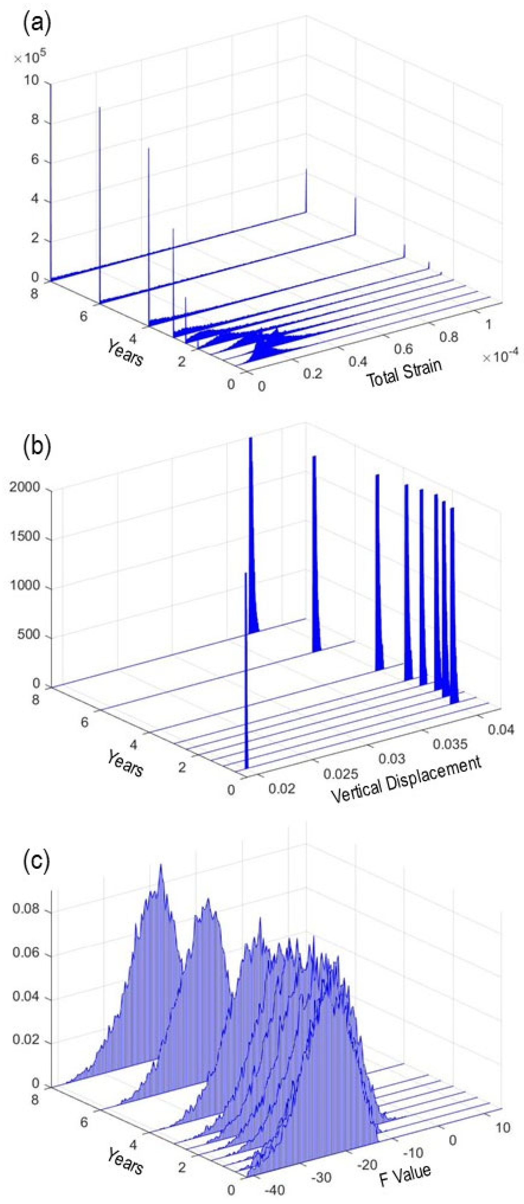
Either PDFs or the corresponding cumulative distribution functions (CDFs) can display the probability distribution in the outcome. A CDF shows the probability level associated with the dependent variable greater than or less than a certain level. Total strain reflects the degree of deformation exerted on the caprock at the injector well location. Given the range/distributions of the input variables, our results indicate that the 50 percentile (P50) or median of the projected equivalent total strain reached a maximum during the initial first year of injection and then gradually decreased and stabilized after the third year of injection (Figure 20). This strain behavior is directly related to the pore pressure development in the aquifer, as plotted in Figure 6. The aquifer pore pressure reached a maximum at year 1 when the plume became well established and reached the first caprock layer, causing localized pore pressure build-up beneath the caprock and associated deformation. As injection continued, the plume grew laterally, and in the process, the pore pressure build-up underneath the caprock became more diffused, resulting in lower total strain in the caprock and eventually stabilizing after year 3 when the average reservoir pressure also stabilized.

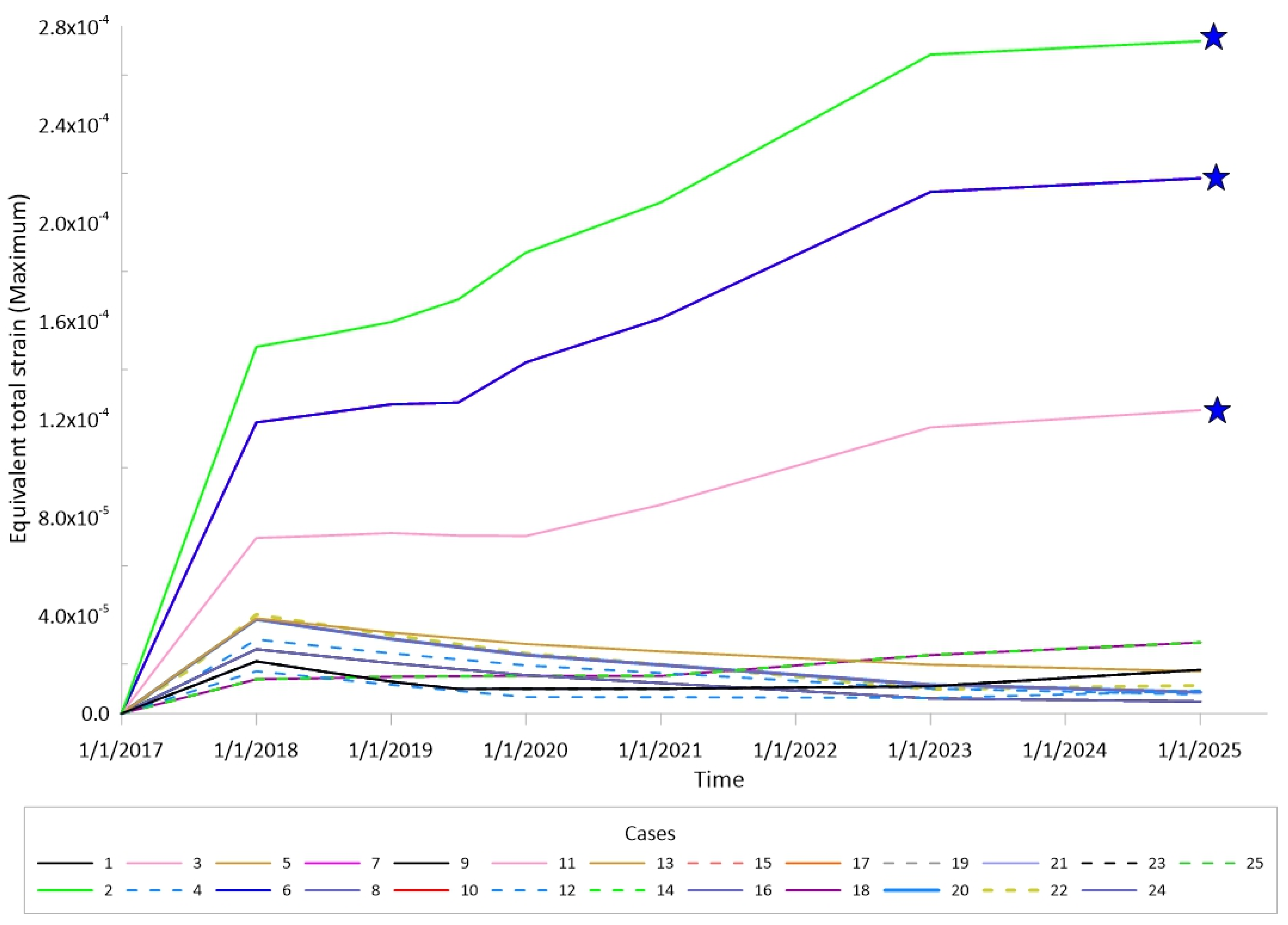
The 75 percentile (P75) above the equivalent total strain was projected to slightly increase after 1 year of injection. Figure 21 illustrates the plot of the maximum equivalent total strain in Caprock 1 for all 25 cases in the BBD. For the vast majority of the cases, the maximum equivalent total strain peaked after 1 year of injection and then decreased before stabilizing after 3 years. However, a small subset of cases (marked with a blue star) show a distinctly different behavior. Their maximum equivalent total strain continued to increase after 1st year of injection, resulting in the divergent pattern noted for P75 and above in Figure 20. On closer examination, these cases represent factorial combinations where the Young modulus of the caprock is at its minimum value (6 Gpa) within its statistical distribution. A low Young’s modulus allows for more ductile behavior, and thus the caprock can accommodate further deformation (strain) beyond the 1st year of injection as marked by star symbols in Figure 21.

Figure 22 shows the predicted maximum vertical displacement at the top of Caprock 1, which follows a similar trend to the equivalent total strain. However, unlike the equivalent total strain and reservoir pressure reaching their peak after 1-year injection, the vertical displacement reached its peak at the 2-year CO₂ injection. This is in response to an overall increase in the pore pressure, which only plateaus after 2 years, as shown in the average reservoir pressure plot in Figure 8 and Table 3. Also, unlike the equivalent total strain, the vertical displacement behavior is remarkably consistent across all cases in the BBD. The probability distribution is very narrow, with P95 of the outcomes within the 0.0412 m increase, and P50 of the results are less than or equal to about 0.0407 m increase at the peak. It is worth noting that the magnitude of equivalent total strains is quite small and as such does not translate into significant variation in the vertical displacement.

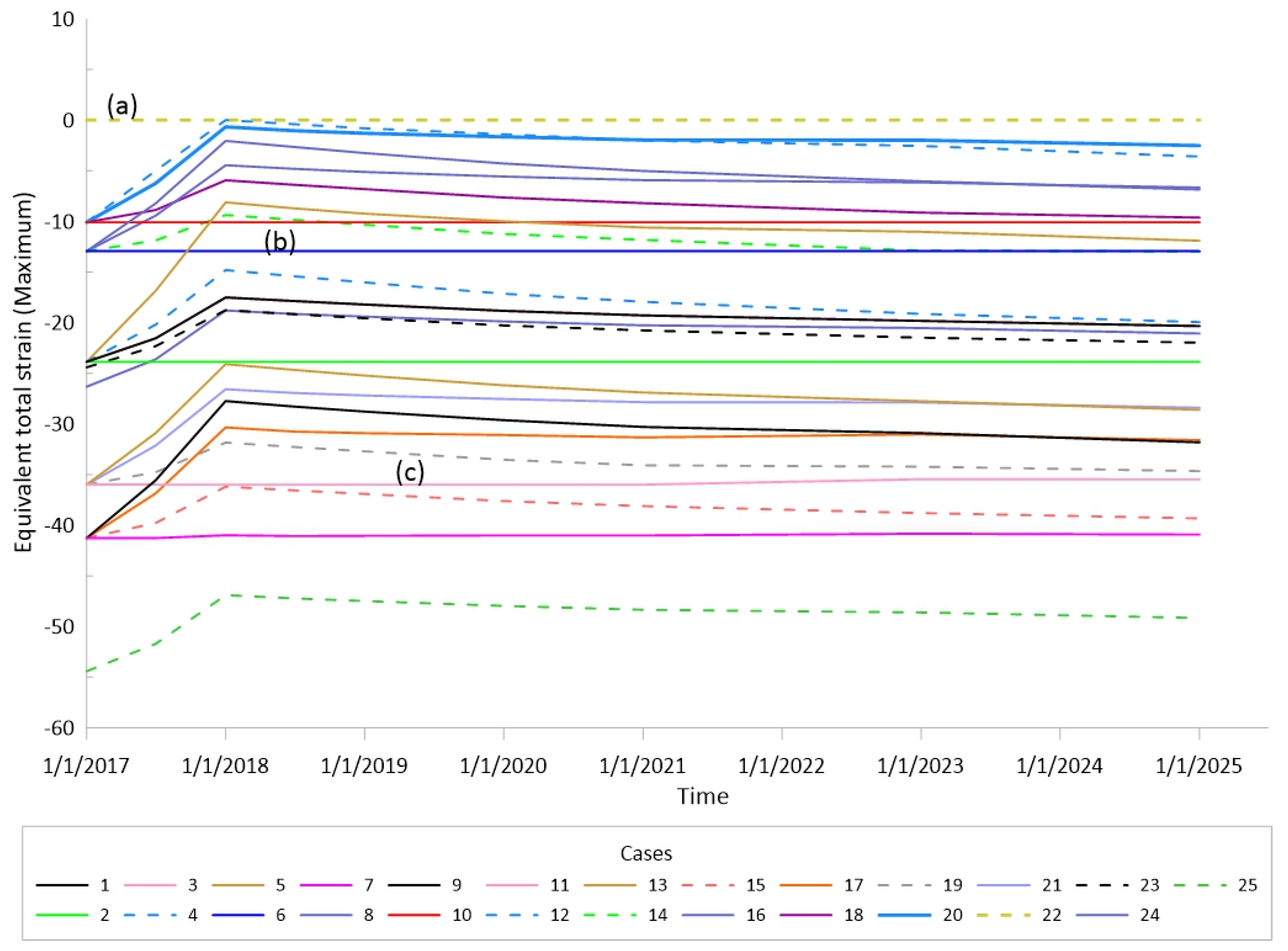
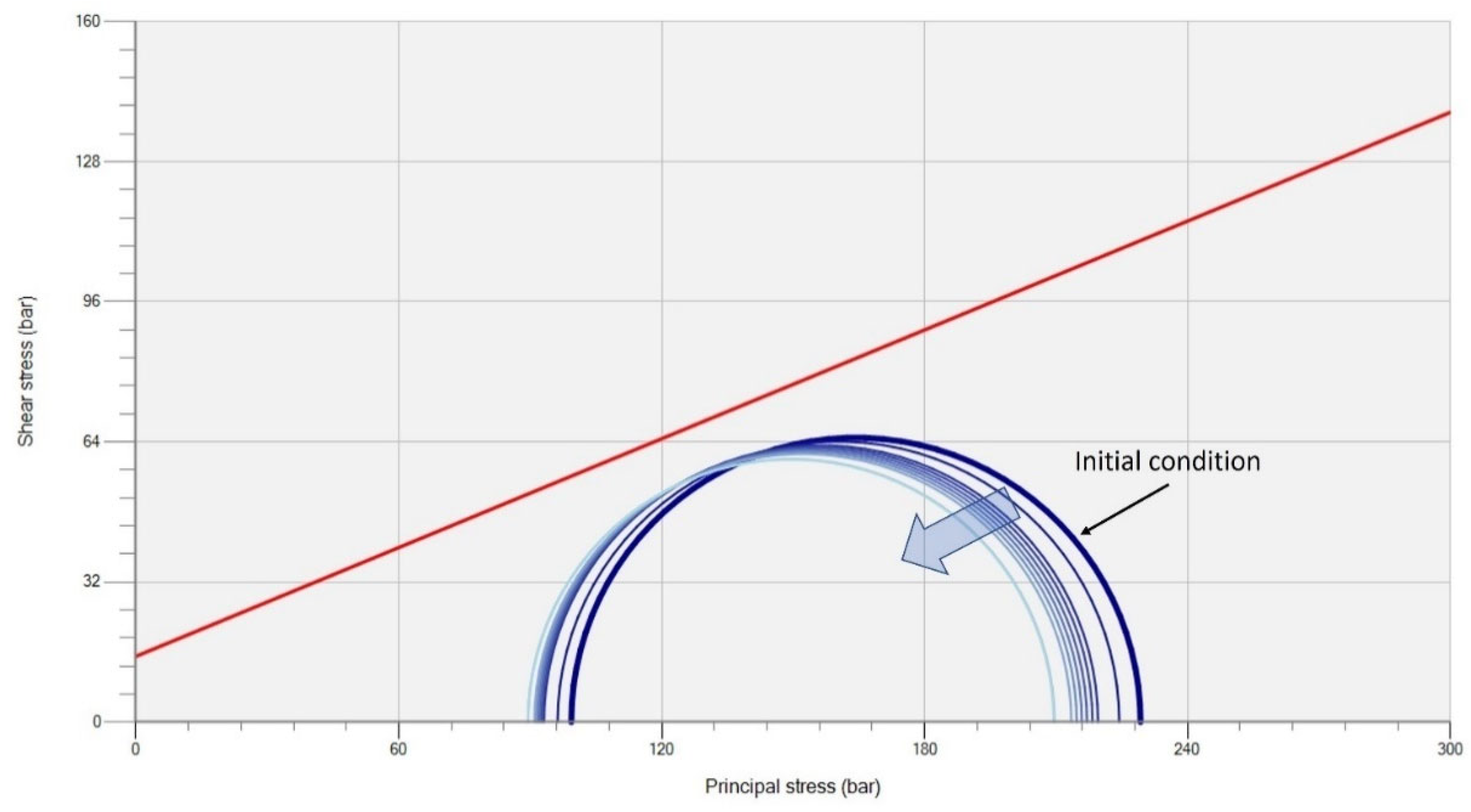
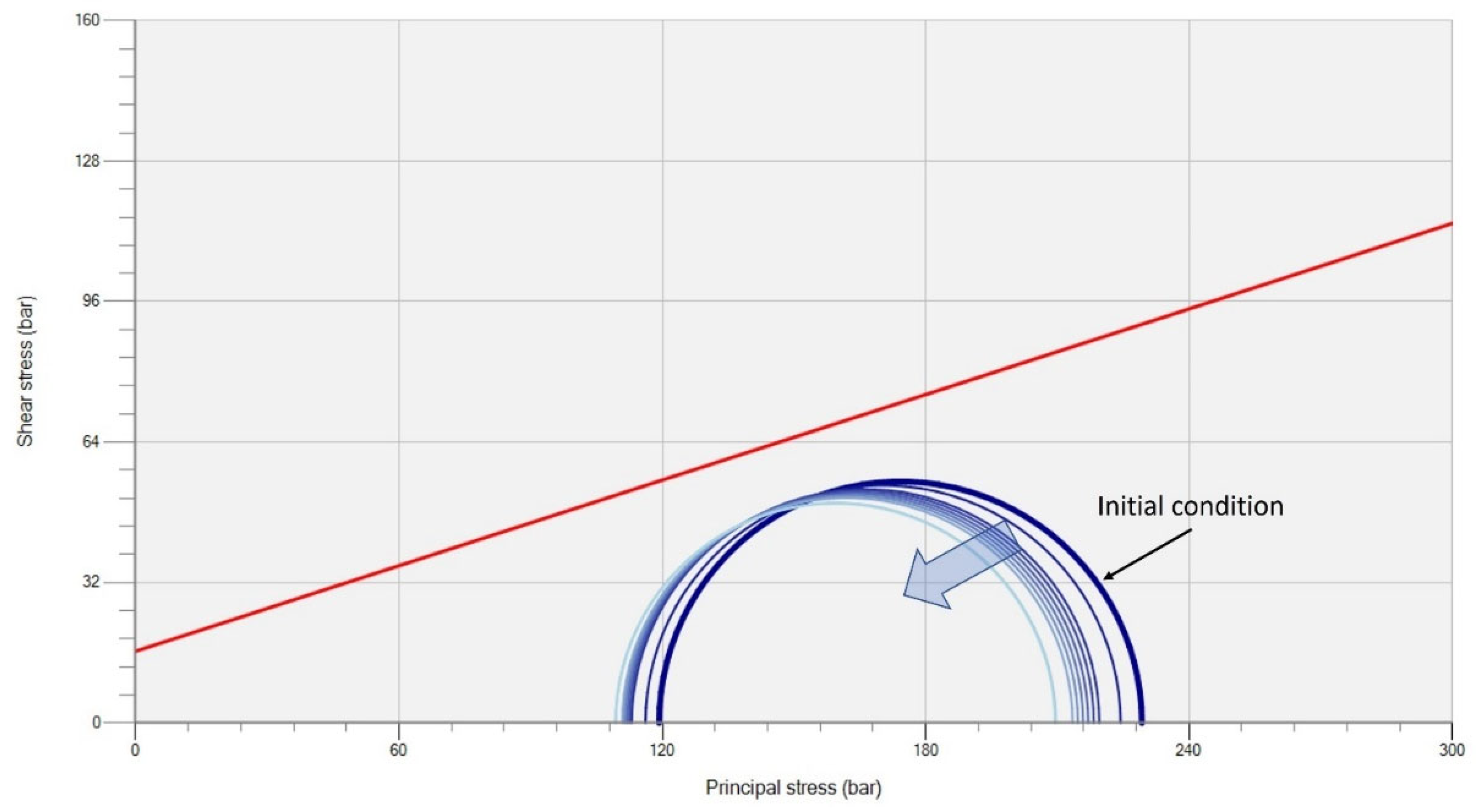
As shown in Figure 23, the 50 percentile (P50) or median of the projected F value increased with CO₂ injection, from a value of (−)24 reaching a maximum value of around (−)18 by the end of the 1-year injection. It then gradually decreased to around (−)19.5 after 8 years of injection. The majority of the 25 cases in the BBD experiment follow this general behavior, as shown in Figure 24. The few exceptions that do not follow this trend are labeled (a), (b), and (c). For (a), the design parameters were such that shear failure had already occurred in the caprock at initial stress conditions prior to any injection (Figure 25), and thus the F value remained at 0. For (b) and (c), the F value remained almost constant because their stress paths followed the gradient of the shear failure envelope (Figure 26 and Figure 27). The probability distribution remained consistent throughout the simulation period with P25 and P75 within 4 bars of P50.

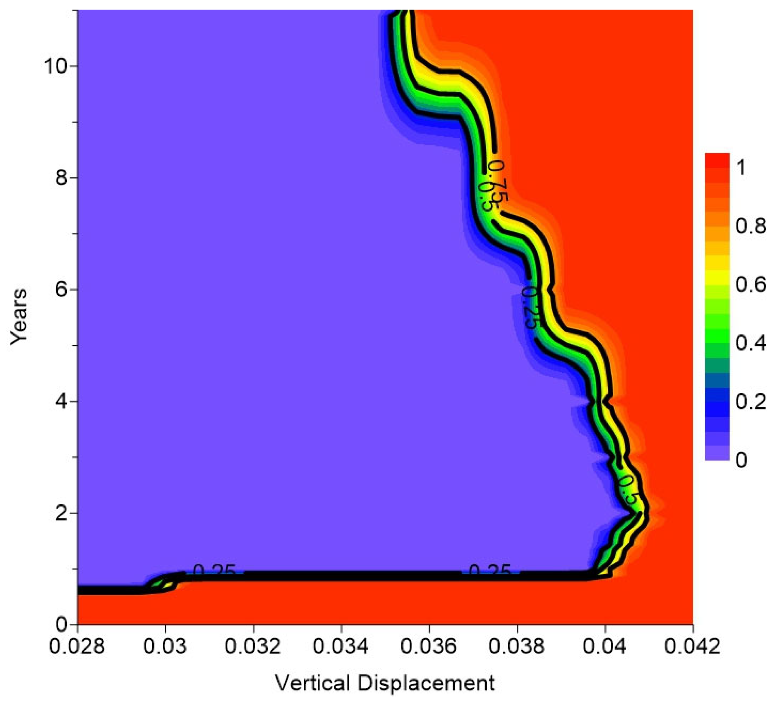
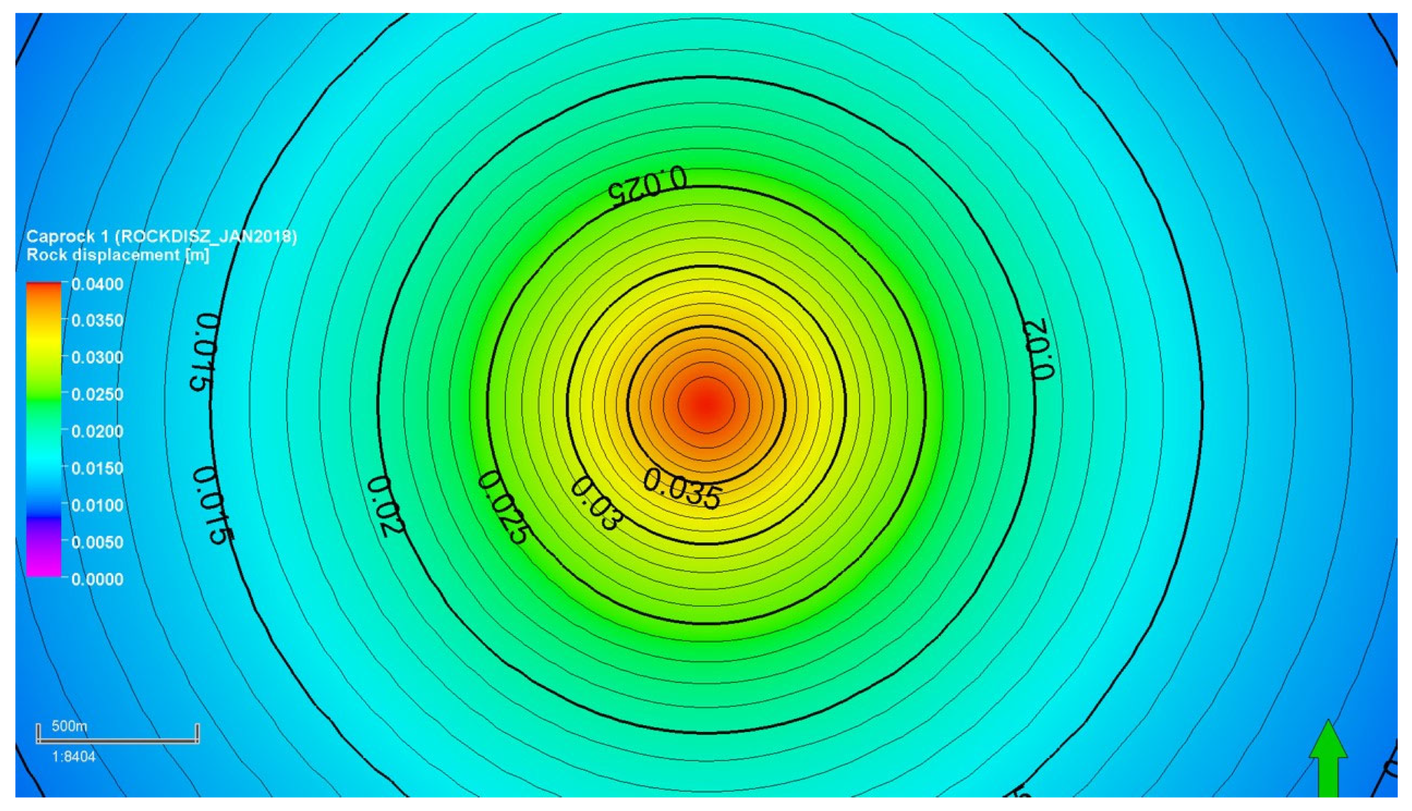
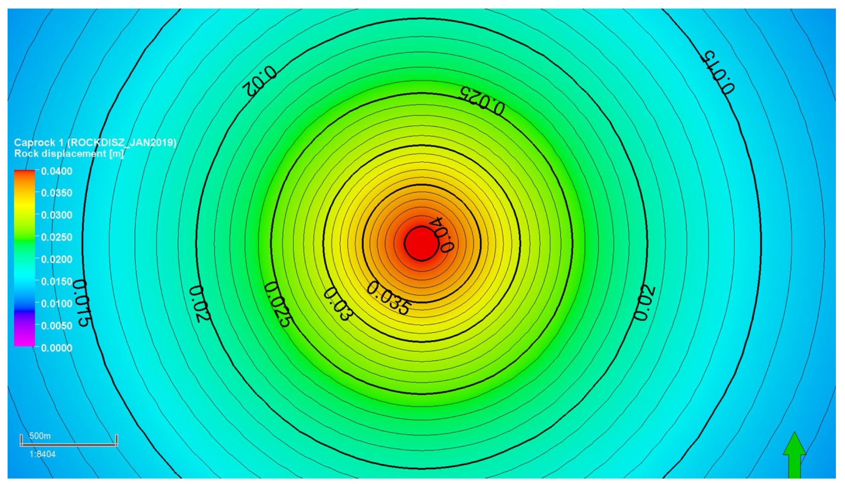
These results indicate that maximum vertical displacement may not be a useful proxy for caprock integrity. Note that the maximum F value was 1 year earlier than the peak of vertical displacement. This can be explained by comparing the vertical displacement maps at 1 year (Figure 28) and 2 years after injection (Figure 29). For this comparison, the results from the base case scenario are used. Although the magnitude of vertical displacement after 1-year injection is less, the contour lines of vertical displacement appear to be closer together, indicating that deformation is more localized and contained within a smaller volume of caprock. At the end of 2 years of injection, the magnitude of vertical displacement is greater, but crucially, deformation is more spread out over a larger area and volume of caprock, as evident from the contour profile. Greater differential vertical displacement within the caprock results in higher strain corresponding to the peak in the equivalent total strain observed for most cases after 1-year injection (Figure 20 and Figure 21).

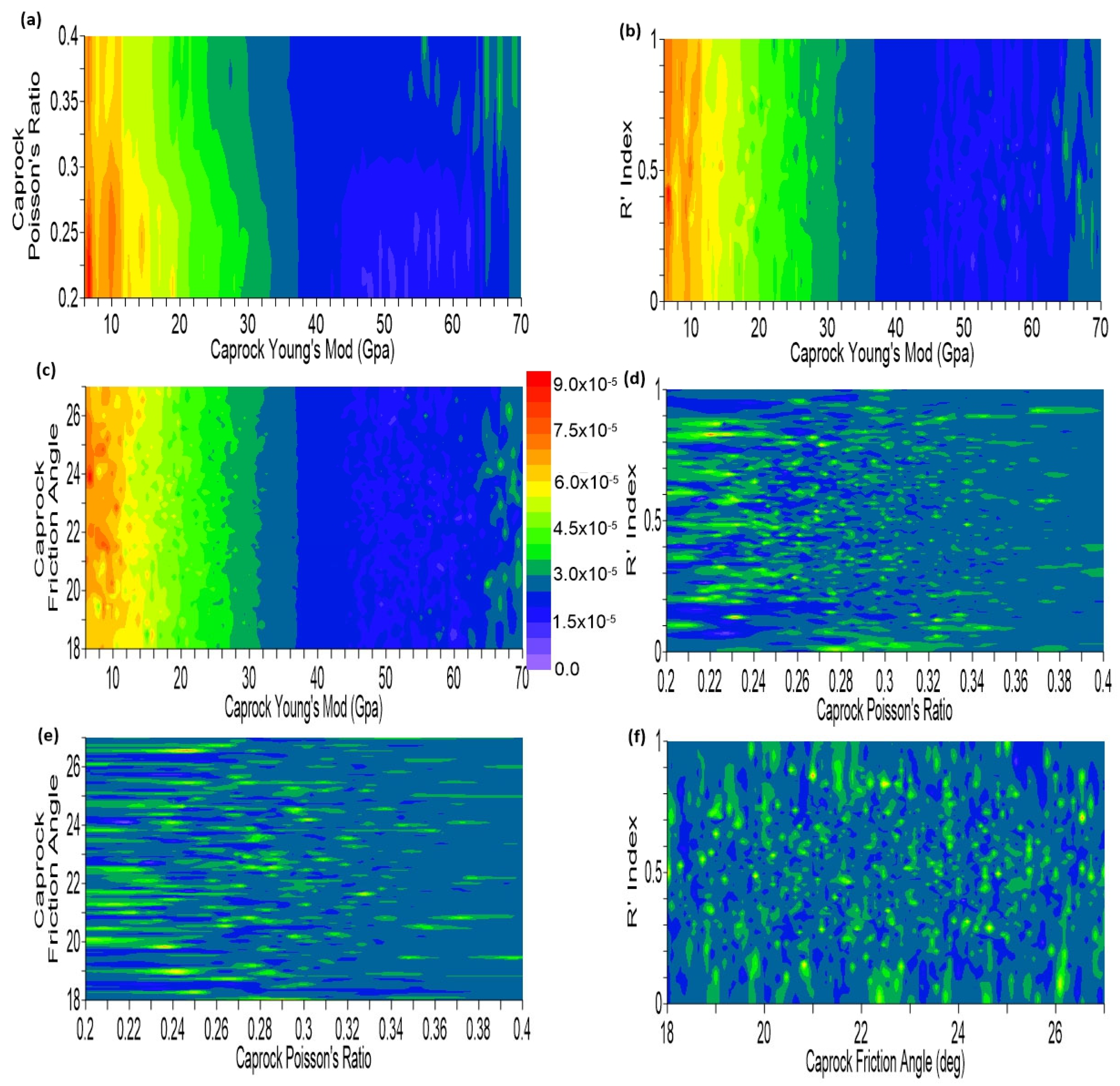
The predicted response of the equivalent total strain, vertical displacement, and F value at 1-year injection, given a combination of independent variables, are plotted in Figure 30, Figure 31 and Figure 32, respectively. The Young modulus of the caprock strongly dictates the magnitude of vertical deformation and the equivalent total strain regardless of the R’ index, the caprock’s Poisson ratio, or friction angle, as evident in Figure 30 and Figure 31. A lower Young’s modulus yields greater equivalent total strain and vertical displacement. The cross-plots of caprock friction angle vs. the caprock’s Poisson ratio, R’ index vs. the caprock’s Poisson ratio, and R’ index vs. the caprock’s friction angle do not yield a predictable response for both equivalent total strain and vertical displacement. This is attributed to the following features:

• Friction angle is a mechanical strength attribute, not an elastic property, and hence does not influence vertical displacement or equivalent total strain.
• Although Poisson’s ratio is an elastic property, it represents the lateral elastic deformation, which is absent or negligible in the vertical displacement and equivalent total strain.
• R’ index (stress regime) dictates the magnitude of deviatoric stress. Since stress and strain are directionally proportional for a given set of elastic properties, the R’ index does not produce a deformation response (via vertical displacement or equivalent total strain) when plotted against a mechanical strength attribute such as friction angle.

Figure 30. Total strain after 1-year injection: (a) caprock’s Poisson ratio vs. caprock’s Young modulus; (b) caprock’s friction angle vs. caprock’s Young modulus; (c) caprock’s friction angle vs. caprock’s Poisson ratio; (d) R’ index vs. caprock’s Young modulus; (e) R’ index vs. caprock’s Poisson ratio; (f) R’ index vs. caprock’s friction angle.

Figure 30. Total strain after 1-year injection: (a) caprock’s Poisson ratio vs. caprock’s Young modulus; (b) caprock’s friction angle vs. caprock’s Young modulus; (c) caprock’s friction angle vs. caprock’s Poisson ratio; (d) R’ index vs. caprock’s Young modulus; (e) R’ index vs. caprock’s Poisson ratio; (f) R’ index vs. caprock’s friction angle.

Figure 31. Vertical displacement after 1-year injection: (a) caprock’s Poisson ratio vs. caprock’s Young modulus; (b) caprock’s friction angle vs. caprock’s Young modulus; (c) caprock’s friction angle vs. caprock’s Poisson ratio; (d) R’ index vs. caprock’s Young modulus; (e) R’ index vs. caprock’s Poisson ratio; (f) R’ index vs. caprock’s friction angle.

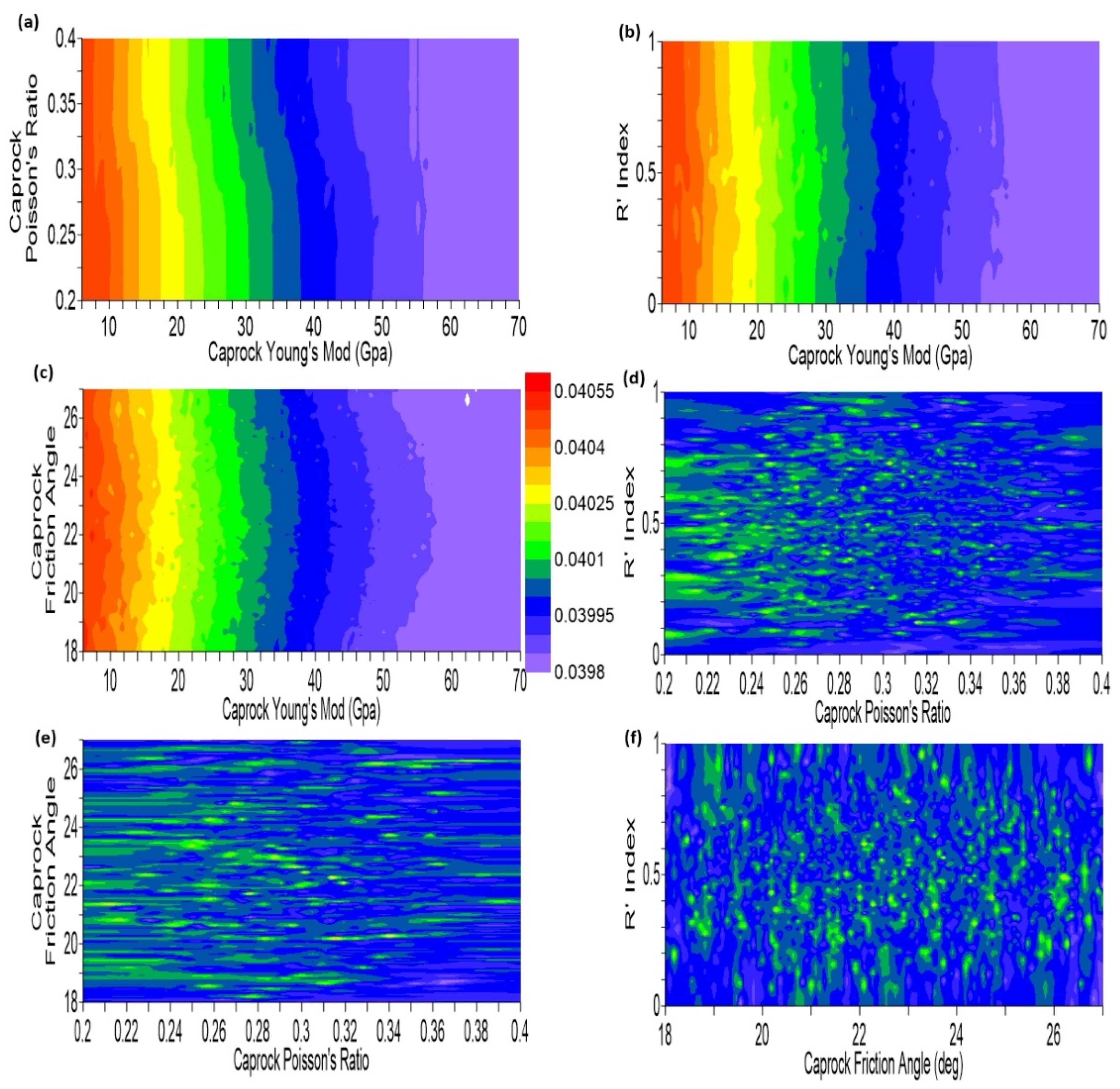
Figure 31. Vertical displacement after 1-year injection: (a) caprock’s Poisson ratio vs. caprock’s Young modulus; (b) caprock’s friction angle vs. caprock’s Young modulus; (c) caprock’s friction angle vs. caprock’s Poisson ratio; (d) R’ index vs. caprock’s Young modulus; (e) R’ index vs. caprock’s Poisson ratio; (f) R’ index vs. caprock’s friction angle.

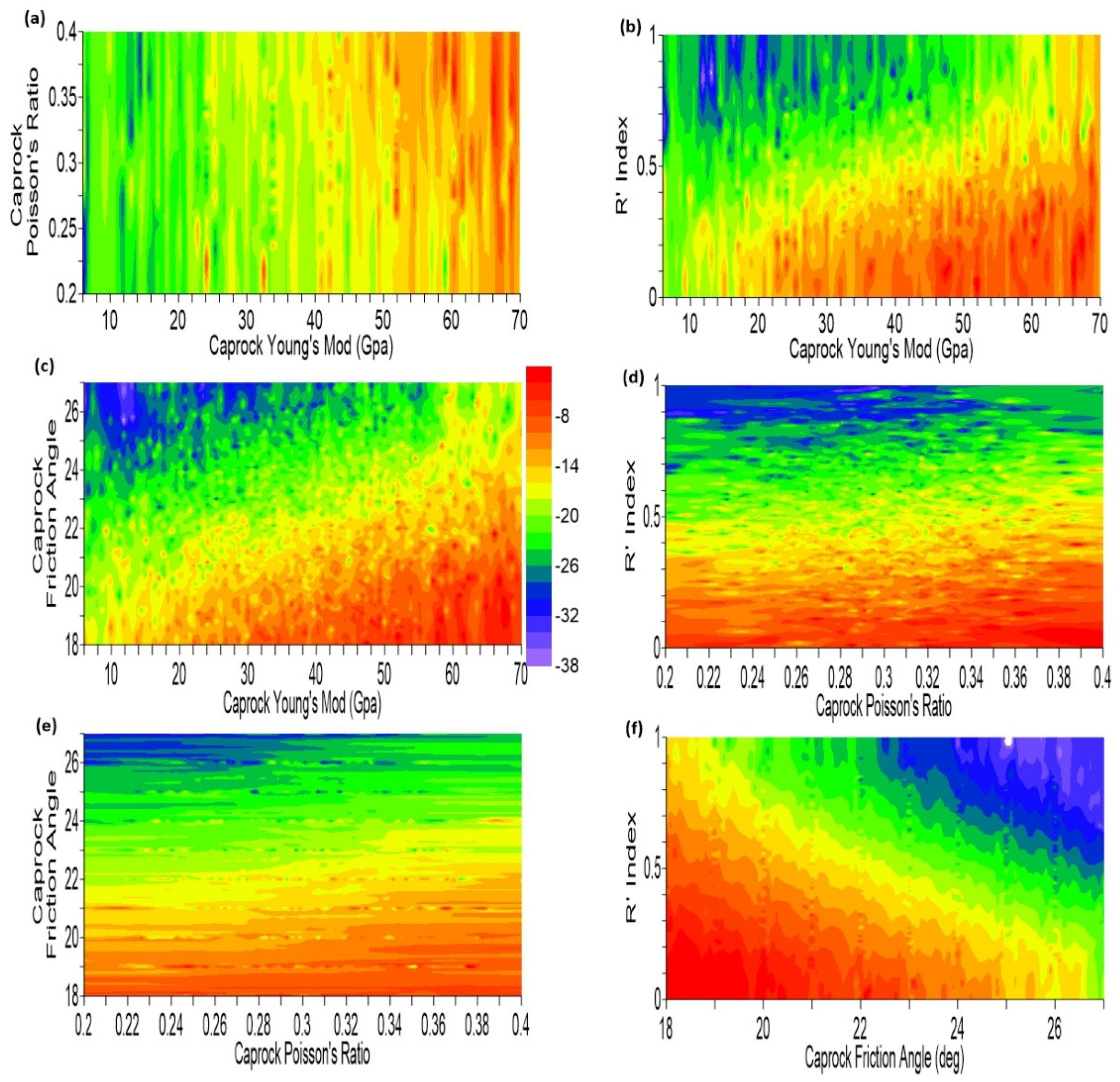
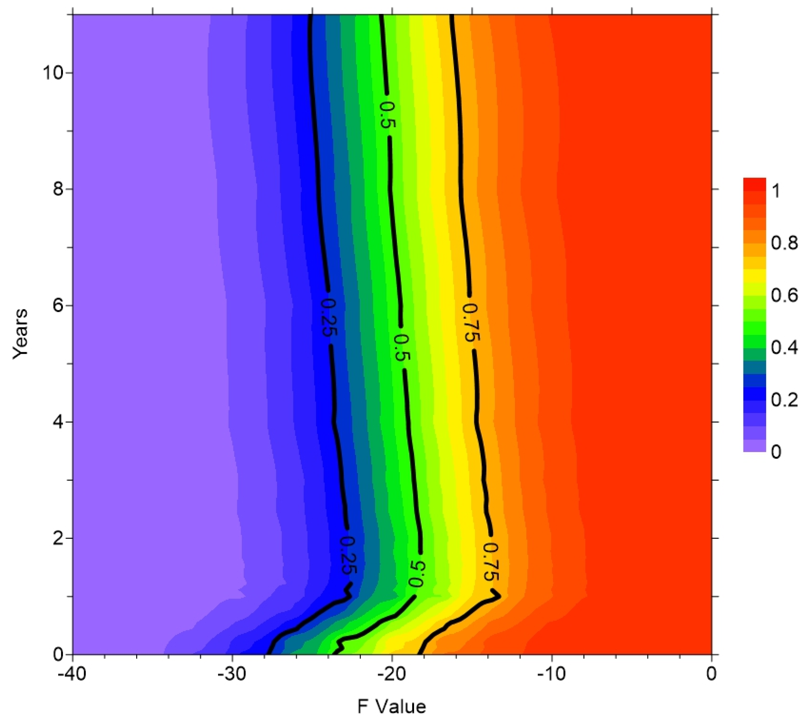
Figure 32. F value after 1-year injection: (a) caprock’s Poisson ratio vs. caprock’s Young modulus; (b) caprock’s friction angle vs. caprock’s Young modulus; (c) caprock’s friction angle vs. caprock’s Poisson ratio; (d) R’ index vs. caprock’s Young modulus; (e) R’ index vs. caprock’s Poisson ratio; (f) R’ index vs. caprock’s friction angle.

Figure 32. F value after 1-year injection: (a) caprock’s Poisson ratio vs. caprock’s Young modulus; (b) caprock’s friction angle vs. caprock’s Young modulus; (c) caprock’s friction angle vs. caprock’s Poisson ratio; (d) R’ index vs. caprock’s Young modulus; (e) R’ index vs. caprock’s Poisson ratio; (f) R’ index vs. caprock’s friction angle.

As shown in Figure 32, the friction angle and Young’s modulus are equally strong drivers for the F value response. A combination of decreasing friction angle and increasing Young’s modulus probabilistically results in a higher F value and a greater risk of caprock integrity failure. Poisson’s ratio is a much weaker driver than both Young’s modulus and the friction angle. Generally, a higher Poisson’s ratio drives greater horizontal loading/expansion of the formation, inducing greater horizontal stress anisotropy. Increasing Poisson’s ratio coupled with increasing Young’s modulus (stiffer rock) or decreasing friction angle (lower shear strength) would likely induce shear failure in the horizontal plane. However, since injection-induced deformation primarily occurs in the vertical component, the horizontal shear component of the caprock failure is minor. A clear trend in the R’ index is also evident; a low R’ index predictively results in a higher F value. This is consistent with the earlier findings from the sensitivity analysis. Rock deformation increased with deviatoric stress (the difference between maximum and minimum principal stresses), resulting in a stress path toward the shear failure envelope. The deviatoric stress was higher in the extensive stress regime (R’ index approaching 0) and gradually decreased toward the strike–slip regime (R’ index approaching 1). A combination of a low R’ index (approaching 0) with an increase in the caprock’s Young modulus and/or a decrease in the caprock’s friction angle probabilistically results in a higher F value and a greater risk of caprock integrity failure.

The predicted response of the equivalent total strain (Figure 30) and vertical displacement (Figure 31) show similar patterns and behavior. This is not surprising since both represent physical deformation but not necessarily rock failure. Given such a range of uncertainty in rock properties, the F value would be a more reliable predictor for caprock integrity failure, especially when the stress regime is known or bound within a narrow range. Figure 32 can serve as a useful primary screening tool to first understand the caprock integrity risk landscape, identifying the riskiest combination of rock properties under different stress regimes. The corresponding probabilistic equivalent total strain (Figure 30) and vertical displacement (Figure 31) can then be referenced in a more meaningful way as part of a field monitoring program.

5. Conclusions

This study presents a probabilistic evaluation of geomechanical risk associated with CO₂ injection, using a simplified hypothetical geological model. Our methodology combines a multilaminate model, a response surface model (RSM) utilizing the Box–Behnken design (BBD), respective numerical experiments, and Monte Carlo simulations. This approach integrates probability distributions to assess variability and uncertainty in risk prediction estimates pertaining to CO₂ storage. It facilitates effective preinjection risk analysis and can be easily updated with new data during and post-injection stages. Additionally, this methodology can be applicable to site screening, project management, monitoring plans, optimization, and risk mitigation strategies, given the inherent uncertainty in input parameters. The results of our study lead us to the following main conclusions:

• In our simplified model, the Young modulus of the caprock is a key factor controlling the equivalent total strain. While a low Young’s modulus allows for greater deformation, strain by itself is not a reliable indicator of caprock integrity. For instance, caprocks with a low Young’s modulus combined with high mechanical strength properties can undergo deformation without compromising their integrity. On the other hand, caprocks characterized by both a low Young’s modulus and low mechanical strength properties are at the highest risk of integrity failure.
• Although vertical displacement is informative, it is not a definitive indicator of caprock integrity. With the uncertainties surrounding Young’s modulus and mechanical strength properties, caprock integrity failure can manifest across a spectrum of vertical displacement values. Differential vertical displacement over a specific rock volume, which indicates localized deformation, is a more predictive metric for caprock failure.
• The most accurate indicator to gauge caprock integrity failure is the F value. Although theoretical, this computational attribute would be the primary parameter in evaluating geomechanical and caprock integrity risks, supported by probabilistic models of the equivalent total strain and vertical displacement.
• Stress regime significantly influences the background deviatoric stress levels, with maximum deviatoric stress observed in both extensive and compressive regimes, and minimum in the strike–slip regime. Although real-world uncertainty in stress regimes is anticipated to be more constrained, our approach satisfactorily produced probability distributions that account for this uncertainty.
• The multilaminate framework offers a simplified yet insightful representation of rock behavior, especially beneficial for fractured rocks. Its integration with the Mohr–Coulomb constitutive model allows for capturing variability in fracture geometries without undue computational complexity.