Abstract
Building automation systems installed in large commercial buildings record sub-hourly measurements from hundreds of sensors. The use of such large datasets are challenging because of missing and erroneous data, which can prevent the development of accurate prediction models of the performance of heating, ventilation, and air-conditioning equipment. The use of the transfer learning (TL) method for building applications attracted researchers to solve the problems created by small and incomplete datasets. This paper verifies the hypothesis that the deep neural network models that are pre-trained for one chiller (called the source chiller) with a small dataset of measurements from July 2013 could be applied successfully, by using TL strategies, for the prediction of the operation performance of another chiller (called the target chiller) with different datasets that were recorded during the cooling season of 2016. Measurements from a university campus are used as a case study. The results show that the initial hypothesis of this paper is confirmed.
1. Introduction
Heating, ventilation, and air-conditioning (HVAC) equipment such as chillers and fans has an important impact on the energy use and electrical demand of large commercial and institutional buildings. Building automation systems (BAS) that are installed in such buildings can record measurements of hundreds of sensors, usually at 15 min time intervals. After the measurement datasets are validated, two kinds of problematic situations could be noticed, which are obstacles for the development, validation, and application of the prediction models:
- (i)
- Datasets for the training of prediction models are small or incomplete;
- (ii)
- Datasets normally available at 15 min time intervals are not sufficient for capturing and analyzing the transient changes of operation conditions, which might happen within a few minutes.
Different approaches have been used for the augmentation of recorded datasets [1,2]. Elaborated mathematical models have been applied to generate new datasets by extrapolating small datasets with faults or by adding artificial faults.
The recent use of the transfer learning (TL) method for building applications has opened up new alternative solutions to problems created by small and incomplete datasets. This paper explores the application of TL for the performance prediction of chillers in a central cooling plant serving a university campus, using the measurement datasets from the BAS as a case study. This section presents briefly the concept of transfer learning and some details about the hyper-parameters of deep learning models.
1.1. Transfer Learning
When the prediction of the energy performance of HVAC equipment, such as a large-capacity chiller, is required, the usual approach consists first of collecting measurements over a time interval, as long as reasonably possible and cost-effective. The dedicated prediction model is then developed and tested, followed by the application. However, in many situations, the available measurements dataset is not adequate for the purpose of model development, either because the dataset is incomplete, some readings are erroneous, or variables needed are not recorded.
In this situation, the transfer learning (TL) method can help in the development of performance prediction models for HVAC equipment.
Transfer learning is used to improve a learner in a target domain by transferring knowledge obtained from a different but related source domain [3]. Another definition simply says that TL is the ability of a system to recognize and apply knowledge and skills learned in previous tasks to novel tasks [4].
When the size and quality of the target training dataset are not sufficient, TL uses a pre-trained model from the source domain as the starting point for the generalization to the target domain. Thus, the application of TL from a source domain to a target domain reduces the need for large task datasets for model training and validation, as well as the training time.
Transfer learning is formally defined by [3] as follows: Given a source domain DS with a corresponding source task TS and a target domain DT with a corresponding target task TT, transfer learning is the process of improving the target predictive function by using the related information from DS and TS, where the two domains are different (DS ≠ DT) or tasks are different (TS ≠ TT).
A few definitions are presented here for the clarification of the method proposed in the paper.
When both the source and the target domains use the same metrics, the transfer learning is called homogeneous, while when the domains use different metrics, the transfer learning is called heterogeneous.
The form of homogeneous transfer learning between the source and target domains can be classified into four transfer categories [4,5]:
- (1)
- Instance-based transfer learning can be used when samples in the source domain are reweighted in an attempt to correct for marginal distribution differences. The reweighted samples are directly used for training in the target domain. For instance, [6] calculated the weights by using the means of the target and source domains.
- (2)
- Feature-based transfer learning, which takes one of the following two different approaches. The first approach, called asymmetric feature transformation, works well when both source and target domains have the same labels and transforms the features of the source through reweighting to more closely match the target domain. The second approach discovers underlying meaningful structures between the domains and transfers both domains to a common feature space.
- (3)
- Model parameter-based transfer learning starts by using parameters (i.e., weights of the deep neutral network (DNN) model), which were trained previously from a source domain, to initialize the weights of the target domain DNN model. Finally, the weights are fine-tuned for the target domain.
- (4)
- Relation-based transfer learning, which uses the common relationship between the source and target domains.
There are three common transfer learning scenarios [3] in terms of task similarity and the availability of labeled datasets [5]:
- (1)
- Inductive transfer learning occurs when the source and target domain data are available and the source and target tasks are different.
- (2)
- Transductive transfer learning occurs when only the source data are available; the source and target domains are different but have the same tasks.
- (3)
- Unsupervised transfer learning occurs when the source and target data are not available and the source and target have different tasks.
A few examples of application of the transfer learning method are listed herein: the detection of faults in chillers [6,7], the forecasting of building energy demand [8,9], the control of HVAC systems [10,11], the detection of faults in solar photovoltaic modules [12], the detection of gas path faults across the turbine fleet [13], the forecasting of indoor air temperature [14], and the building information extraction [15]. The detailed literature review of applications of transfer learning to HVAC systems is beyond the scope of this paper.
Liu et al. [6] used a laboratory-controlled set-up of two chillers, the source chiller with a 422 kW (120 tons) cooling capacity and the target chiller with a 703 kW (200 tons) cooling capacity. The paper presented the results of applying two transfer learning strategies to a convolutional neural network (CNN) model used for FDD: (a) with complete source chiller working data, and (b) with partial data available. Several approaches were used, starting with the original pre-trained CNN model of the source chiller and applying it to the target chiller:
- (i)
- by using the pre-trained model without any fine-tuning; and
- (ii)
- using the pre-trained model for weight initialization, and then (b1) fine-tuning the weights of all layers, and (b2) fine-tuning only the weights of fully connected layers.
The results showed that (i) the performance obtained with fine-tuning of all layers was better than that with fine-tuning only fully connected layers; and (ii) the models trained on data from a particular source chiller are difficult to use directly with the target chiller. The results also revealed that the amount of source domain data does not have a significant impact on the improvement of the transfer learning model. However, the more data in the source domain, the better the stability of the model.
Fan et al. [7] presented the development of an FDD model of a target chiller by using the support vector machine (SVM) with imbalanced datasets in size and diversity. The knowledge from one source water-cooled chiller of 422 kW (120 tons) capacity [6] with a large dataset of normal and fault operations was applied to a target water-cooled chiller of 703 kW (200 tons) capacity with a smaller dataset. The use of prior knowledge from the source chiller along with the adaptive imbalanced processing enlarged the datasets of normal and fault situations, which helped for better diagnostic performance of the FDD model of the target chiller.
Qian et al. [8] presented the improvement of daily and monthly forecasting of seasonal cooling loads in a building, which combined the load simulation with the EnergyPlus program with transfer learning, using only a small amount of available data. The simulation dataset of 15–21 July 2009 was used for training and validation, and the dataset of cooling season May–October 2010 was used as the target. An instance-based transfer learning strategy was applied. The results indicated that the transfer learning strategy could improve forecasting accuracy when compared with conventional load forecasting methods such as ANN.
Fan et al. [9] presented a transfer learning method for 24 h ahead forecasting of building energy demand, using as a case study 407 buildings randomly selected as the source domain and other 100 buildings as the target domain. The usefulness of transfer learning was evaluated by using two learning scenarios and different implementation strategies. First, a pre-trained baseline model was developed from the source domain operational data. Then, the knowledge learned by the pre-trained model was transferred to target buildings using two implementation strategies: (i) feature extraction, where all the model weights are fixed except for the output layer or the last few layers; and (ii) weight initialization, where the weights of the pre-trained model are used for initialization only and are fine-tuned.
Two learning scenarios are simulated: (a) the training data available is insufficient; and (b) the building data are available but cannot adequately describe building operating conditions. The results obtained with scenario (a) showed that the value of the pre-trained model decreased with the increase in training data amounts. More stable results can be obtained when utilizing the pre-trained model for weight initialization. The results in scenario (b) showed that the value of the pre-trained model tends to increase with the increase in training data amounts.
Zhu et al. [10] presented a framework for transferring the prior knowledge of an information-rich source screw chiller to build the diagnostic model for a new screw target chiller. Domain adaptation transfer learning is applied to overcome the differences in feature distribution between chillers. An adversarial neural network generated the diagnostic model for the target chiller, which has only easy-to-collect normal operation data along with the prior knowledge from the source chiller. Results indicated that the transferred diagnostic model for the target chiller yields decent diagnostic performance. The proposed transfer learning approach has improved performance compared with conventional machine learning models.
Coraci et al. [11] used a homogeneous transductive TL to transfer a Deep Reinforcement Learning control policy of the cooling system from one source building to various target buildings by using hourly synthetic data from a simulation environment that coupled EnergyPlus and Python. The target buildings were derived from the source building by varying the weather conditions, electricity price schedules, occupancy schedules, and building thermophysical properties. The pre-trained control model of the source building was fine-tuned for each target building. The weight-initialization TL method was used as a knowledge-sharing strategy between source and target buildings.
Reference [12] used TL with convolutional neural network (CNN) models to detect faults in solar photovoltaic modules. A CNN model was pre-trained using a dataset of thermographic infrared PV images of various anomalies found in solar systems, and the IR images are separated according to different fault classes. The offline augmentation method was used to increase the classification success in the case of a low number of fault images. The model was re-trained to extract multi-scale feature maps to classify anomalies. The results from the proposed method show that the average improvement could reach about 24% compared with the conventional model training strategy.
Li et al. [13] proposed a method that is capable of learning transferable cross-domain features while preserving the properties and structures of the source domain as much as possible. The method was applied to the detection of gas path faults across the turbine fleet. The goal was to complete the diagnostic task of the target domain with the help of fault knowledge learned from the source domain.
Bellagarda et al. [14] tested different TL methods applied to neural network models for the forecasting of indoor air temperature in existing buildings. The results indicate that the implementation of TL contributed to an extension of the forecast horizon by 13.4 hours on average. The model’s performance maintains acceptable accuracy in 79% of the cases.
Wang et al. [15] applied TL along with deep neural networks to improve the query from building information modeling (BIM). They achieved a high precision of 99.76% on the validation dataset.
1.2. Deep Learning
Deep learning (DL) is a machine learning method [16]. An example of a DL model is the multilayer perceptron (MLP), composed of a mathematical function (that may consist of many simpler functions) mapping some sets of input values to output values, where each application of a different mathematical function can be regarded as providing a new representation of the input.
DL refers to machine learning models that include multi-levels of nonlinear transformation. Deep neural network (DNN) models are the application of such strategies to neural networks [17].
Figure 1 shows the multilayer perceptron (MLP) as a fully connected DNN model, as an example, for the prediction task with three sequential layers: (1) one input layer including n inputs, (2) three hidden layers, and (3) one output layer including m outputs. Each layer is composed of adjustable neurons, where the number of neurons in the input layer usually depends on the number of independent inputs, and the number of neurons in the output layer depends on the number of predicted target variables.
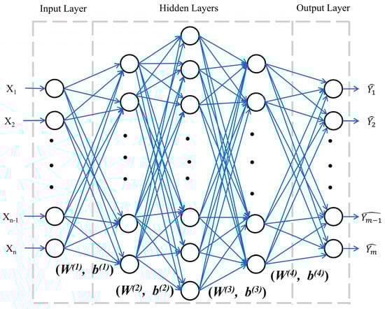
Figure 1.
Deep neural network model architecture.
DNN is a type of feed-forward neural network; the summation of inputs with corresponding weights and biases (e.g., W(1) and b(1) in Figure 1) is sent to the first hidden layer and goes through a non-linear transformation due to the activation function applied. The information from the first hidden layer, along with corresponding weights and biases, is sent to the next hidden layer for another non-linear transformation, following the feedforward process. Equations (1)–(3) are listed as examples.
where h(1) and h(2) are the outputs of the first and second hidden layers, g is the activation function, is the output of the output layer, and WT and b are the weights and biases of the corresponding hidden layer.
A few examples of recent publications (2015–2022) that focused on prediction or classification tasks are listed in Table 1. A detailed literature review of the application of DNN in the field of HVAC systems is beyond the scope of this paper.

Table 1.
Examples of the architecture of deep neural networks in the literature review of 2015–2022.
Important hyperparameters of the DNN model are the number of hidden layers and the number of neurons in each hidden layer. A DNN model with more hidden layers usually outperforms the one with only one hidden layer in some aspects, like greater accuracy and preventing overfitting. All reviewed papers used between two and six hidden layers. However, there is not a general rule to set the number of hidden layers, except for the recommendation found in [18]. Each hidden layer has either an equal or unequal number of neurons. The activation function of the rectified linear unit (ReLU) is used in seven papers, while four other papers do not give information about the activation functions (marked as NA in Table 1).
According to [18], the best performance and robustness of a DNN model could be achieved with: (i) two hidden layers; (ii) the number of neurons in the first hidden layer equal to 2 × (2 × n + 1), where n is the number of neurons in the input layer; and (iii) the number of neurons in the second hidden layer equal to (2 × n + 1).
1.3. Objective: Hypothesis Testing
This paper verifies the hypothesis that the DNN models that are pre-trained for one chiller (called the source chiller) with a small dataset of measurements from 14 days in July 2013 could be applied successfully, by using TL strategies, for the prediction of the operation performance of another chiller (called the target chiller) with different datasets, which were recorded three years later, during the cooling season of 2016. Measurements, recorded by the BAS of a university campus, are used as a case study.
The measurement datasets, obtained from BAS, are recorded every 15 min. This short time interval brings a larger variation of data compared with the hourly or monthly measurement data or with synthetic data. The use of BAS trend data are also more challenging in terms of missing data, noise, and erroneous data than using data from laboratory-controlled conditions or synthetic data. Hence, achieving high performance in transfer learning in this study becomes more challenging.
The paper proposes the use of homogeneous transductive TL between the source chiller and target chiller, with a few strategies for weight initialization. The prediction performance of DNN models is evaluated over a few validation datasets of the target chiller, and the effect of TL is discussed.
The paper is structured as follows: Section 2 presents the method proposed for the application of transfer learning to the case study of existing chillers. Section 3 presents details of the case study based on measurements from the BAS. Section 4 presents the architecture of DNN models for the prediction of target variables and the training and validation datasets. Section 5 presents the discussion of the results. Chapter 6 presents the conclusions from the case study of transfer learning.
2. Method
2.1. Transfer Learning Strategies
The homogeneous transductive transfer of information between two domains is staged as follows:
- (a)
- from the source domain or source chiller (SD) that has measurement data to be used for the pre-training and validation of DNN models,
- (b)
- to the target domain or target chiller (TD) that has measurement data to be used for the re-training (fine-tuning) of DNN models and for the validation of updated models.
This paper evaluates three transfer learning strategies applied to the case study:
- TLS0: The DNN model is pre-trained and tested with the dataset of SD, and then it is used directly with the dataset of TD without changing the initial model weights. TLS0 is also called the direct TL. The DNN model’s performance is evaluated with the validation dataset of TD.
- TLS1: The DNN model is first pre-trained and tested with the dataset of SD, and then it is updated using the dataset of TD. The weights of all DNN model layers are fine-tuned with the training dataset of TD. The updated DNN model is evaluated with the validation dataset of TD.
- TLS2: The DNN model is first pre-trained and tested with the dataset of SD, and then it is updated with the dataset of TD. Only the weights of the output layer are updated. The updated DNN model is evaluated with the validation dataset of TD.
In addition to the above three transfer learning strategies, another DNN model is developed by using the so-called self-learning (SelfL) strategy. This model is trained and tested only with the TD dataset.
2.2. Structure of Deep-Neural Network (DNN) Models
This paper uses DNN models for transfer learning (TL); one DNN model is built to predict each selected target operation variable of chillers.
The dataset is normalized to the range of 0 to 1 by using the min-max normalization method, as it is suitable for data with known bounds and without many outliers [29]. (Equation (4)).
where Xi,norm is the normalized value of Xi, Xmin is the minimum value, and Xmax is the maximum value.
The analysis of measurements in this case study revealed that the time lag effect is not significant in the development of DNN models for the steady-state operation of chillers. For this reason, the multiple layer perceptron (MLP) is selected as the DNN model instead of a time-series model (e.g., LSTMs).
The DNN models are implemented using Python (version 3.9.12) [30] with open libraries like TensorFlow (version 2.10.0) [31]. The optimum hyper-parameters of five DNN models, i.e., the activation function and learning rate, are identified by trial-and-error. For each DNN model, the iteration is set for 10,000 epochs, and the optimum activation function (Table 2) is selected from the following list: ReLU [32], eLU, GeLU [33], SeLU [34,35], sigmoid, and tanh (Equations (5)–(10)) (Table 3). The optimum learning rate (Table 2) is selected from the following list: 0.001, 0.01, 0.1, 0.2, 0.4, 0.6, 1.
Table 2.
Selected activation function and learning rate for each DNN model.
Table 3.
Activation functions.
The model training stops when one of the two criteria has been met: (1) the mean square error of the output (target) variable over the training dataset has fallen under the value listed in Table 2, or (2) the maximum number of iterations of 10,000 epochs has been reached. The criterion for stopping the model training was identified by trial-and-error.
The algorithm of stochastic gradient descent with momentum [36,37] (Equations (11) and (12)) is applied to tune the weights of DNN models. The loss function (Equation (13)) is used to estimate the loss of the model over the training dataset so that the weights can be updated iteratively to reduce the loss [38].
where:
where M represents weights, l is the learning rate, β is the momentum constant, is the gradient, and k equals to the length of training dataset.
The prediction results are compared with measurements, and the model performance is evaluated with three performance metrics: (i) the root-mean square error, RMSE; (ii) the coefficient of variation of RMSE, CV(RMSE); and (iii) the mean absolute deviation (MAD) [39] that is used when the RMSE metric is sensitive to large errors (Equation (14)).
According to Guideline 14 [40], the calibration of a computer model of a single building is acceptable if the CV(RMSE) between the measurements and predictions of the whole-building energy use is smaller than 30% when using hourly data or smaller than 15% when using monthly data.
By extension of [40], some authors have applied such benchmarks of CV(RMSE) to other conditions, such as the virtual water flow meter [41]. Thus, the CV(RMSE) values are calculated in this paper from the difference between measurements of the target chiller and predictions of DNN models using TL and then compared with the thresholds of [40].
3. Case Study
The case study uses BAS trend data from a central cooling and heating plant that serves the chilled water loop of a university campus [42]. Measurements data were collected from two vapor compression, water-cooled chillers named CH#1 and CH#2. At design conditions, they have an equal cooling capacity of 3165 kW (900 tons of refrigeration), a coefficient of performance (COP) of 5.76, and an electric power input of 549.5 kW [43]. They use low-pressure R-123 refrigerant. At design conditions, the chilled water leaves at 5.6 °C and returns at 13.3 °C, and the condenser water temperature enters the cooling tower at 35.0 °C and leaves at 29.4 °C. Chiller CH#1 or CH#2 starts first by rotation, trying to balance the number of operating hours over the life span of each chiller, or for maintenance reasons. When the first chiller starts, the corresponding chilled-water and condenser-water pumps start too. The second chiller starts only if the first chiller cannot meet the chilled-water demand.
Chillers were installed in 2007, and some changes in the operation parameters were made starting in 2008. For instance, the measured chilled-water temperature supply changed in 2009 from 5.6 °C (the design value) to 6.8 °C, and the COP was calculated as 5.29 (CH#1) and 5.39 (CH#2), compared with the design value of 5.76. Details about the operation and performance of these two chillers are available in [43].
The pre-processing of raw measurements was used to verify the quality of the raw data [44]. Three kinds of data were removed, including (1) obvious abnormal values (e.g., negative values of Vchw when the chiller operates normally), (2) the data under transient conditions (e.g., chiller start-up), and (3) outliers that exceed Chauvenet’s criterion [39].
4. Modeling
4.1. Measurement Data Sets
In this paper, the transfer learning method uses the source domain (SD) data, which is composed of measurements data over July 2013 at 15 min time intervals (14 days for pre-training and two days for validation of DNN models), when the chiller CH#2 worked alone.
In many publications, a large dataset of measurements is used for model training. However, we plan to test the hypothesis that a smaller data set can also be used along with TL. The knowledge (i.e., DNN models) extracted from SD is transferred to the target domain (TD) for the application with the measurement data of the target chiller, CH#1. Measurements available from the target chiller CH#1 are from June to August 2016, when the chiller CH#1 worked alone. Data from TD is used for the re-training and validation of the DNN models.
Five DNN models are developed, one for each target operation variable of chillers (E, COP, Tcdwl, ΔTchw, and ΔTcdw), using as inputs the directly measured or derived variables (Table 4). The chiller energy balance relationships were analyzed to select the required inputs for each model [45]. Several correlation-based models between the target variable and regressors were evaluated [46]. For instance, the best correlation was obtained between COP, a target variable, and four independent variables (Tchwl, Vchw, PLR, mev, and refr).
Table 4.
Architecture of each deep neural network model.
4.2. Training and Validation of DNN Models
The DNN models are first trained using SD data (CH#2) of 14 days (11 July to 24 July 2013) and validated with SD data of two days (25–26 July 2013) (Table 5).
Table 5.
Source domain datasets and target domain datasets of type #1 of short duration.
The re-training of DNN models over the target domain (CH#1) uses either short duration (type #1) or long duration (type #2) validation datasets of TD to verify if the transfer learning (TLS0, TSL1, TLS2, and SelfL) strategies along with DNN models are successful:
- (i)
- Type #1 of short-duration datasets. For instance, the re-training of DNN models is made with data TD1 of two days (22 June to 23 June 2016) and the validation with data of four days (from 27 June to 30 June 2016) (Table 5).
- (ii)
- Type #2 of long-duration datasets. For instance, the re-training of DNN models is made with data from TD4 of two days (22 June to 23 June 2016) and the validation with data from 16 days (from 27 June to 12 August 2016) (Table 6).
Table 6. Source domain datasets and target domain datasets of type #2 of long duration.
Each dataset in SD and TD contains the same set of variables, including Tchwr, Tchwl, ΔTchw, Vchw, mev,refr, Tev, Tcd, Tdis, E, PLR, COP, Tcdwr, Tcdwl, and ΔTcdw.
5. Results and Discussion
The two chillers were selected with identical design values, but sooner after the installation some operating values were changed. The measurements data proved differences between the training datasets of CH#2 (2013) and CH#1 (2016) (Table 7). For instance, the COP of target chiller CH#1 is greater than the value of source chiller CH#2, while Tchwl, Vchw, and E (except for TD3) values are smaller than the values of source chiller CH#2. The refrigerant temperature at the condenser Tcd of CH#1 is smaller by up to 5 °C than the value of CH#2. The measurement uncertainty in Table 7 was calculated according to ASHRAE Guideline 2 [47].
Table 7.
Comparison of average values and uncertainty of directly measured and derived variables of the training datasets of the source chiller (CH#2) and target chiller (CH#1).
5.1. Pre-Training and Validation of DNN Models Using the Source Domain Data (CH#2, 2013)
First, the performance metrics of DNN models, one for each target variable, are estimated when they are pre-trained and validated with the source domain data (SD) (CH#2, 2013). The performance metrics of each DNN model are displayed in Table 8, along with the measurement uncertainty (Um) of each target variable.
Table 8.
Performance metrics of five DNN models, one for each target variable, using the source domain data (SD) (CH#2, 2013).
All RMSE values over the validation data are smaller than the uncertainty values, except in the case of electric power input to the chiller (E) of 23.48 kW, which is only slightly greater than the measurement uncertainty of 19.02 kW. The reason could be the recording of a few large differences between measurement and prediction values of E, which have an important impact on the RMSE once they are raised to a power of two. For the comparison, the MAD value (Equation (14)) is smaller than the uncertainty value.
The learning curves represented by the variation of mean square error with the number of epochs on both the training dataset and validation dataset of SD are presented in Figure 2, which takes the DNN model of E as an example.
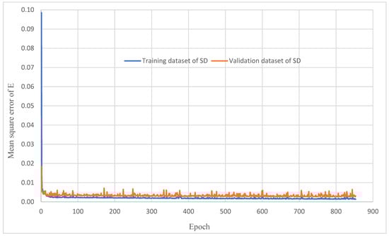
Figure 2.
Learning curve over both the training dataset and the validation dataset of SD.
In conclusion, all five DNN models, one for each target variable, which are pre-trained with SD data (CH#2, 2013), predict the target variables well over the validation dataset of SD.
5.2. Results of Transfer Learning Strategies Applied to the Target Domain Datasets of Type #1 of Short Duration (CH#1, 2016)
This section discusses the results from the application of transfer learning strategies along with type #1 short-duration datasets of the target chiller (CH#1).
The results of the self-learning (SelfL) strategy, which uses the DNN models that were trained and validated with the datasets of TD (CH#1, 2016), are used as benchmarks for comparison with other transfer learning strategies. Both the TLS1 and TLS2 strategies, which use the pre-trained models with the source dataset, followed by the re-tuning of the weights with the target datasets, perform better than the TLS0 strategy (which uses the pre-trained model weights without any modification) and the Self strategy.
All MAD values (Table 9) corresponding to TLS1 and TLS2 are smaller than the measurements uncertainty, except for the case of E in TD1. The difference between the performance metrics of TLS1 and TLS2 is negligible.
Table 9.
MAD metric of TL strategies over the type #1 target validation datasets (TD1, TD2, and TD3) with respect to DNN models of E and COP.
Although all values of CV(RMSE) (Table 10) are below 30%, which is acceptable for measurements at 15 min time intervals, the TLS1 and TLS2 strategies have better performance, as indicated by the CV(RMSE) values, compared with the results of the SelfL and TSL0 strategies.
Table 10.
CV(RMSE) of TL strategies over the type #1 target validation datasets (TD1, TD2, and TD3) with respect to DNN models of E and COP.
In conclusion, when the transfer learning strategies TLS1 and TLS2, which use the pre-trained models with the source dataset, followed by the re-tuning of the weights with the target datasets, are applied to TD validation datasets of type #1 of short duration, they give better predictions of target values (E and COP) than the other two TL strategies (i.e., TLS0 and SelfL).
5.3. Results of Transfer Learning Strategies Applied to the Target Domain Datasets of Type #2 of Long Duration (CH#1, 2016)
This section discusses the results from the application of transfer learning strategies along with type #2 long-duration datasets of the target chiller (CH#1, 2016).
The five DNN models (E, COP, Tcdwl, ΔTchw, and ΔTcdw), derived with the training dataset of the source chiller (CH#2), are transferred over three datasets (TD4, TD5, and TD6) of the target chiller. The strategies presented in Section 4.2 are also used in this section.
The performance metrics MAD and CV(RMSE) of the DNN models of the target variables E and COP, obtained by using the four TL strategies, are shown in Table 11 and Table 12, respectively. The TLS1 strategy has slightly better performance compared with other strategies.
Table 11.
MAD of SelfL, TLS0, TLS1, and TLS2 over validation datasets of three TDs (TD4, TD5, and TD6) with respect to DNN models of E and COP.
Table 12.
CV(RMSE) of TL strategies over the type #2 target validation datasets (TD4, TD5, and TD6) with respect to DNN models of E and COP.
6. Conclusions
The results of this case study led to the following conclusions:
- The initial hypothesis of this paper is confirmed. The DNN models of the source chiller (CH#2), which are pre-trained with a small dataset of measurements from July 2013, predict well, by using TL strategies, the operation performance of the target chiller (CH#1) when compared with measurements datasets from 2016.
- The pre-training of DNN models plays an important role in the transfer of learning from the source chiller to the target chiller. Transfer learning strategies TLS1 or TLS2 perform better than TLS0 or SelfL. Updating the weights of DNN models with the target data helps improve the performance of DNN models over the validation datasets of TD.
- When the DNN models of the target chiller are trained and validated by using only the target data (SelfL strategy), without having the benefit of previous knowledge from the source chiller, the predictions are generally less accurate.
- There is no numerical evidence from this case study that the TLS1 strategy (i.e., the weights of all DNN model layers are updated) is significantly better than the TLS2 strategy (i.e., only the weights of the output layer are updated).
- Results with target data sets of type #2 (long duration) reveal that by using only 2–5 days of re-training the DNN models, the TLS1 and TLS2 strategies help for good predictions over the course of 3–4 weeks of summer 2016.
- Results from this study support those by [6]. The models trained on data from a particular source chiller cannot be used directly with the target chiller (in our case, this is the strategy TLS0).
This study concluded on the successful application of the transfer learning method for the case study of two chillers based on measurements of two different years from BAS.
The results apply only to this case study. Future work is needed to generalize, if possible, the conclusions to various chillers of different models, cooling capacities, operation controls, and manufacturers. The collaboration of researchers, building owners, utility companies, and manufacturers, which have measurements datasets similar to those used in this paper, is essential for future work on the transfer learning method for HVAC systems in large buildings. The method presented in this paper can be implemented in Building Automation Systems to add new features to the ongoing commissioning of HVAC systems in large commercial and institutional buildings. The proposed method should also be tested for its application to fault detection and diagnosis of HVAC systems.
Author Contributions
Conceptualization, H.D. and R.Z.; methodology, H.D. and R.Z.; validation, H.D. and R.Z.; investigation, H.D.; resources, R.Z.; data curation, H.D.; writing—original draft preparation, H.D.; writing—review and editing, R.Z. and H.D.; supervision, R.Z.; project administration, R.Z.; funding acquisition, R.Z. All authors have read and agreed to the published version of the manuscript.
Funding
This research was funded by the Natural Sciences and Engineering Research Council (NSERC) Discovery Grants (Grant no. RGPIN/2021-04030) and the Gina Cody School of Engineering and Computer Science of Concordia University (VE-0017).
Data Availability Statement
Data is available upon request.
Conflicts of Interest
The authors declare no conflict of interest.
References
- Lashgari, E.; Liang, D.; Maoz, U. Data augmentation for deep-learning-based electroencephalography. J. Neurosci. Methods 2020, 346, 108885. [Google Scholar] [CrossRef] [PubMed]
- Feng, J.; Li, Y.; Zhao, K.; Xu, Z.; Xia, T.; Zhang, J.; Jin, D. DeepMM: Deep Learning Based Map Matching with Data Augmentation. IEEE Trans. Mob. Comput. 2022, 21, 2372–2384. [Google Scholar] [CrossRef]
- Weiss, K.; Khoshgoftaar, T.M.; Wang, D.D. A survey of transfer learning. J. Big Data 2002, 3, 9. [Google Scholar] [CrossRef]
- Pan, S.J.; Yang, Q. A Survey on Transfer Learning. IEEE Trans. Knowl. Data Eng. 2009, 22, 1345–1359. [Google Scholar] [CrossRef]
- Pinto, G.; Wang, Z.; Roy, A.; Hong, T.; Capozzoli, A. Transfer learning for smart buildings: A critical review of algorithms, applications, and future perspectives. Adv. Appl. Energy 2022, 5, 100084. [Google Scholar] [CrossRef]
- Liu, J.; Zhang, Q.; Li, X.; Li, G.; Liu, Z.; Xie, Y.; Li, K.; Liu, B. Transfer learning-based strategies for fault diagnosis in building energy systems. Energy Build. 2021, 250, 111256. [Google Scholar] [CrossRef]
- Fan, Y.; Cui, X.; Han, H.; Lu, H. Chiller fault detection and diagnosis by knowledge transfer based on adaptive imbalanced processing. Sci. Technol. Built Environ. 2020, 26, 1082–1099. [Google Scholar] [CrossRef]
- Qian, F.; Gao, W.; Yang, Y.; Yu, D. Potential analysis of the transfer learning model in short and medium-term forecasting of building HVAC energy consumption. Energy 2020, 193, 116724. [Google Scholar] [CrossRef]
- Fan, C.; Sun, Y.; Xiao, F.; Ma, J.; Lee, D.; Wang, J.; Tseng, Y.C. Statistical investigations of transfer learning-based methodology for short-term building energy predictions. Appl. Energy 2020, 262, 114499. [Google Scholar] [CrossRef]
- Zhu, X.; Chen, K.; Anduv, B.; Jin, X.; Du, Z. Transfer learning based methodology for migration and application of fault detection and diagnosis between building chillers for improving energy efficiency. J. Affect. Disord. 2021, 200, 107957. [Google Scholar] [CrossRef]
- Coraci, D.; Brandi, S.; Hong, T.; Capozzoli, A. Online transfer learning strategy for enhancing the scalability and deployment of deep reinforcement learning control in smart buildings. Appl. Energy 2023, 333, 120598. [Google Scholar] [CrossRef]
- Korkmaz, D.; Acikgoz, H. An efficient fault classification method in solar photovoltaic modules using transfer learning and multi-scale convolutional neural network. Eng. Appl. Artif. Intell. 2022, 113, 104959. [Google Scholar] [CrossRef]
- Li, B.; Zhao, Y.-P.; Chen, Y.-B. Learning transfer feature representations for gas path fault diagnosis across gas turbine fleet. Eng. Appl. Artif. Intell. 2022, 111, 104733. [Google Scholar] [CrossRef]
- Bellagarda, A.; Cesari, S.; Aliberti, A.; Ugliotti, F.; Bottaccioli, L.; Macii, E.; Patti, E. Effectiveness of neural networks and transfer learning for indoor air-temperature forecasting. Autom. Constr. 2022, 140, 104314. [Google Scholar] [CrossRef]
- Wang, N.; Issa, R.R.; Anumba, C.J. Transfer learning-based query classification for intelligent building information spoken dialogue. Autom. Constr. 2022, 141, 104403. [Google Scholar] [CrossRef]
- Goodfellow, I.; Bengio, Y.; Courville, A. Deep Learning; MIT Press: Cambridge, MA, USA, 2016. [Google Scholar]
- Runge, J. Short-Term Forecasting for the Electrical Demand of Heating, Ventilation, and Air Conditioning Systems. Ph.D. Thesis, Concordia University, Montreal, QC, Canada, 2021. [Google Scholar]
- Benedetti, M.; Cesarotti, V.; Introna, V.; Serranti, J. Energy consumption control automation using Artificial Neural Networks and adaptive algorithms: Proposal of a new methodology and case study. Appl. Energy 2016, 165, 60–71. [Google Scholar] [CrossRef]
- Lee, K.-P.; Wu, B.-H.; Peng, S.-L. Deep-learning-based fault detection and diagnosis of air-handling units. J. Affect. Disord. 2019, 157, 24–33. [Google Scholar] [CrossRef]
- Khalil, A.J.; Barhoom, A.M.; Abu-Nasser, B.S.; Musleh, M.M.; Abu-Naser, S.S. Energy Efficiency Prediction using Artificial Neural Network. Int. J. Acad. Pedagog. Res. 2019, 3, 1–7. Available online: https://philpapers.org/rec/KHAEEP (accessed on 31 October 2022).
- Ayadi, M.I.; Maizate, A.; Ouzzif, M.; Mahmoudi, C. Deep Learning in Building Management Systems over NDN: Use case of Forwarding & HVAC Control. In Proceedings of the 2019 International Conference on Internet of Things (IThings) and IEEE Green Computing and Communications (GreenCom) and IEEE Cyber, Physical and Social Computing (CPSCom) and IEEE Smart Data (SmartData), Atlanta, GA, USA, 14–17 July 2019; pp. 1192–1198. Available online: https://ieeexplore.ieee.org/stamp/stamp.jsp?tp=&arnumber=8875410 (accessed on 31 October 2022).
- Chen, Y.; Tong, Z.; Zheng, Y.; Samuelson, H.; Norford, L. Transfer learning with deep neural networks for model predictive control of HVAC and natural ventilation in smart buildings. J. Clean. Prod. 2020, 254, 119866. [Google Scholar] [CrossRef]
- Ali, U.; Shamsi, M.H.; Bohacek, M.; Purcell, K.; Hoare, C.; Mangina, E.; O’donnell, J. A data-driven approach for multi-scale GIS-based building energy modeling for analysis, planning and support decision making. Appl. Energy 2020, 279, 115834. [Google Scholar] [CrossRef]
- Park, H.; Park, D.Y. Comparative analysis on predictability of natural ventilation rate based on machine learning algorithms. J. Affect. Disord. 2021, 195, 107744. [Google Scholar] [CrossRef]
- Esrafilian-Najafabadi, M.; Haghighat, F. Occupancy-based HVAC control using deep learning algorithms for estimating online preconditioning time in residential buildings. Energy Build. 2021, 252, 111377. [Google Scholar] [CrossRef]
- Al-Shargabi, A.A.; Almhafdy, A.; Ibrahim, D.M.; Alghieth, M.; Chiclana, F. Tuning Deep Neural Networks for Predicting Energy Consumption in Arid Climate Based on Buildings Characteristics. Sustainability 2021, 13, 12442. [Google Scholar] [CrossRef]
- Olu-Ajayi, R.; Alaka, H.; Sulaimon, I.; Sunmola, F.; Ajayi, S. Building energy consumption prediction for residential buildings using deep learning and other machine learning techniques. J. Build. Eng. 2022, 45, 103406. [Google Scholar] [CrossRef]
- Wang, M.; Wang, Z.; Geng, Y.; Lin, B. Interpreting the neural network model for HVAC system energy data mining. J. Affect. Disord. 2022, 209, 108449. [Google Scholar] [CrossRef]
- Fausett, L. Fundamentals of Neural Networks: Architectures, Algorithms and Applications, 1st ed.; Pearson: Bloomington, MN, USA, 1993. [Google Scholar]
- Welcome to Python.org. Available online: https://www.python.org/ (accessed on 3 April 2022).
- Google. “TensorFlow”. Available online: https://www.tensorflow.org (accessed on 22 February 2022).
- Nair, V.; Hinton, G.E. Rectified Linear Units Improve Restricted Boltzmann Machines. In Proceedings of the 27th International Conference on Machine Learning, Haifa, Israel, 21–24 June 2010; Available online: https://www.cs.toronto.edu/~hinton/absps/reluICML.pdf (accessed on 19 January 2023).
- Hendrycks, D.; Gimpel, K. Gaussian Error Linear Units (GELUs). arXiv 2016, arXiv:1606.08415v5. [Google Scholar]
- Ramachandran, P.; Zoph, B.; Le, Q.V. Searching for Activation Functions. arXiv 2017, arXiv:1710.05941v2. [Google Scholar]
- Klambauer, G.; Unterthiner, T.; Mayr, A.; Hochreiter, S. Self-Normalizing Neural Networks. In Proceedings of the 31st Conference on Neural Information Processing Systems, Long Beach, CA, USA, 4–9 December 2017. [Google Scholar]
- Amari, S.-I. Backpropagation and stochastic gradient descent method. Neurocomputing 1993, 5, 185–196. [Google Scholar] [CrossRef]
- Sutskever, I.; Martens, J.; Dahl, G.; Hinton, G. On the importance of initialization and momentum in deep learning. In Proceedings of the 30th International Conference on Machine Learning, Atlanta, GA, USA, 16–21 June 2013. [Google Scholar]
- Brownlee, J. How to Choose Loss Functions When Training Deep Learning Neural Networks. Available online: https://machinelearningmastery.com/how-to-choose-loss-functions-when-training-deep-learning-neural-networks/ (accessed on 20 January 2023).
- Reddy, T.A. Applied Data Analysis and Modeling for Energy Engineers and Scientists; Springer: New York, NY, USA, 2011. [Google Scholar] [CrossRef]
- Guideline 14-2014; Measurement of Energy and Demand Savings. American Society of Heating, Refrigerating and Air-Conditioning Engineers: Peachtree Corners, GA, USA, 2014.
- Qiu, S.; Li, Z.; He, R.; Li, Z. User-friendly fault detection method for building chilled water flowmeters: Field data validation. User-friendly fault detection method for building chilled water flowmeters: Field data validation. Sci. Technol. Built Environ. 2022, 28, 1116–1137. [Google Scholar] [CrossRef]
- Monfet, D.; Zmeureanu, R. Ongoing commissioning approach for a central cooling and heating plant. ASHRAE Trans. 2011, 117, 908–924. [Google Scholar]
- Dou, H.; Zmeureanu, R. Evidence-based assessment of energy performance of two large centrifugal chillers over nine cooling seasons. Sci. Technol. Built Environ. 2021, 27, 1243–1255. [Google Scholar] [CrossRef]
- Han, J.; Pei, J.; Kamber, M. Data Mining: Concepts and Techniques; Elsevier: Amsterdam, The Netherlands, 2011. [Google Scholar]
- Dou, H. Fault Detection and Diagnosis (FDD) for Multiple-Dependent Faults of Chillers. Ph.D. Thesis, Concordia University, Montreal, QC, Canada, 2023. Available online: https://spectrum.library.concordia.ca/id/eprint/992031/ (accessed on 6 September 2023).
- Dou, H.; Zmeureanu, R. Detection and Diagnosis of Multiple-Dependent Faults (MDFDD) of Water-Cooled Centrifugal Chillers Using Grey-Box Model-Based Method. Energies 2023, 16, 210. [Google Scholar] [CrossRef]
- Guideline 2-2010; Engineering Analysis of Experimental Data. American Society of Heating, Refrigerating and Air-Conditioning Engineers, Inc.: Atlanta, GA, USA, 2010.
Disclaimer/Publisher’s Note: The statements, opinions and data contained in all publications are solely those of the individual author(s) and contributor(s) and not of MDPI and/or the editor(s). MDPI and/or the editor(s) disclaim responsibility for any injury to people or property resulting from any ideas, methods, instructions or products referred to in the content. |
© 2023 by the authors. Licensee MDPI, Basel, Switzerland. This article is an open access article distributed under the terms and conditions of the Creative Commons Attribution (CC BY) license (https://creativecommons.org/licenses/by/4.0/).