Anomaly Detection in a Smart Microgrid System Using Cyber-Analytics: A Case Study

Abstract

Smart microgrids are being increasingly deployed within the Department of Defense. The microgrid at Marine Corps Air Station (MCAS) Miramar is one such deployment that has fostered the integration of different technologies, including 5G and Advanced Metering Infrastructure (AMI). The objective of this paper is to develop an anomaly detection framework for the smart microgrid system at MCAS Miramar to enhance its cyber-resilience. We implement predictive analytics using machine learning to deal with cyber-uncertainties and threats within the microgrid environment. An autoencoder neural network is implemented to classify and identify specific cyber-attacks against this infrastructure. Both network traffic in the form of packet captures (PCAP) and time series data (from the AMI sensors) are considered. We train the autoencoder model on three traffic data sets: (1) Modbus TCP/IP PCAP data from the hardwired network apparatus of the smart microgrid, (2) experimentally generated 5G PCAP data that mimic traffic on the smart microgrid and (3) AMI smart meter sensor data provided by the Naval Facilities (NAVFAC) Engineering Systems Command. Distributed denial-of-service (DDoS) and false data injection attacks (FDIA) are synthetically generated. We show the effectiveness of the autoencoder on detecting and classifying these types of attacks in terms of accuracy, precision, recall, and F-scores.

1. Introduction

Industrial control systems (ICSs) serve as the backbone of cyber–physical systems, effectively managing the control and monitoring of sensors and actuators embedded in industrial operations. They regulate power generation, enable industrial automation, and respond to operational fluctuations. A specific ICS subtype, the microgrid, is an assembly of interconnected loads and distributed energy resources functioning as a single controllable entity forming a power grid.

A microgrid is generally composed of renewable and non-renewable distributed energy resources (DER), such as photovoltaic (PV) array units, back-up generators, and battery storage units. These DERs can be used to facilitate different technologies, including electric vehicles (EV) [1]. Microgrids leverage smart sensor technologies, such as advanced metering infrastructure (AMI) to record and transmit power estimation data to a central data concentrator [2]. These digital components control physical processes and network together disparate energy assets through IP-based protocols. Once a system has network connectivity, its risks for cyber-penetration are guaranteed.

Cyber-resilience is a strategy that provides a system with (1) the ability to detect a cyber-threat and (2) once detected, allows the system to adapt to or quickly recover from the attack. The use of cyber-analytics via machine learning to continually define and mitigate evolving threat vectors in a CPS is a proactive approach to cyber-resilience and defense. Machine learning is an effective cyber-analytic approach where an immense amount of data can be analyzed in near real-time leading to effective response management in real time.

In recent years, the Department of Defense (DoD) has come to rely on smart-energy-based CPS for critical tasks. An example of this includes the Navy’s deployment of a smart grid energy management system to ensure networked power communications for base installations [3,4]. Similarly, the Marine Corps Air Station (MCAS) Miramar, located in San Diego, CA, has taken steps to modernize its base energy systems by implementing a basewide smart research microgrid that consists of various DERs and over 200 smart meters.

The research in this paper is associated with the MCAS Miramar smart microgrid system use case and its ability to monitor energy asset performance in real time from a cyber-resilience perspective. Our focus is on the strategy to detect cyber-threats in this system. Recovery from and real time management of the system once threats are detected are not considered in this paper.

1.1. MCAS Miramar Smart Microgrid

The research microgrid deployed at Miramar is the first of its kind on US bases, and it is considered one of the most energy-forward defense installations in the country [5]. The microgrid is operated and controlled directly out of the Energy and Water Operations Center (EWOC). The EWOC is established in one location on base and is the main control hub for all energy control systems and activities [6]. The EWOC is responsible for overseeing DERs, including but not limited to PV array inverters and backup generators located across the base. The EWOC is also the central hub that monitors data from the various AMI smart meters that are spread across the base.

All other non-critical control and management of the research microgrid is performed by an integrated microgrid controller, referred to as the Energy Management System (EMS) [7]. The EMS is managed by Raytheon Technologies. Communications between the EMS and energy asset devices is through the use of the Modbus TCP/IP over Ethernet protocol.

Over 200 AMI smart sensors are also deployed across base buildings to facilitate automated data collection in real time about energy usage. Some smart sensors/meters are directly connected to various DERS, specifically the solar panels located on the roof of base buildings. Most smart meters are isolated to internal building energy operations.

The various DERs that the EWOC currently manages are dispersed across the Miramar base. However, the EWOC does not have remote monitoring and control capabilities of its PV inverters and backup generators, which limits their visibility of DER operational status on a continuous basis [8]. In 2021, MCAS Miramar partnered with US Ignite, a national non-profit, to build and implement an energy communications infrastructure that would allow MCAS Miramar to support smart technology using Internet of Things (IoT) devices [8]. MCAS Miramar and US Ignite leverage wireless communications to connect specific DERs to the EMS located in the EWOC [8]. Specifically, the use of 5G communications was proposed [8].

5G Living Lab

MCAS Miramar hosts a 5G Living Lab (5GLL) program that is powered by Verizon’s 4G LTE/5G Ultra-Wideband (UWB) network [7]. This is a technology pilot program meant to develop applications of 5G that support the DoD mission [7]. The Verizon commercial network (through the 5GLL effort) currently provides ubiquitous 4G LTE connectivity across the base. There are also two dozen small cell nodes that have been installed [7]. The small cell nodes operate in the millimeter wavelength (mmWave) spectrum to provide areas of ultra-high bandwidth and low latency across the base. PV inverters and backup generators located at various buildings on the base are within range of one or more of these small cell nodes [7].

The Verizon 4G LTE/5G network currently deployed at Miramar is a commercial, non-standalone (NSA) network. In the NSA architecture, the control signaling of the 5G radio network is anchored to the 4G core while the radio frequency (RF) channel uses 5G New Radio (NR). 5G NR introduces the use of mmWave for communications.

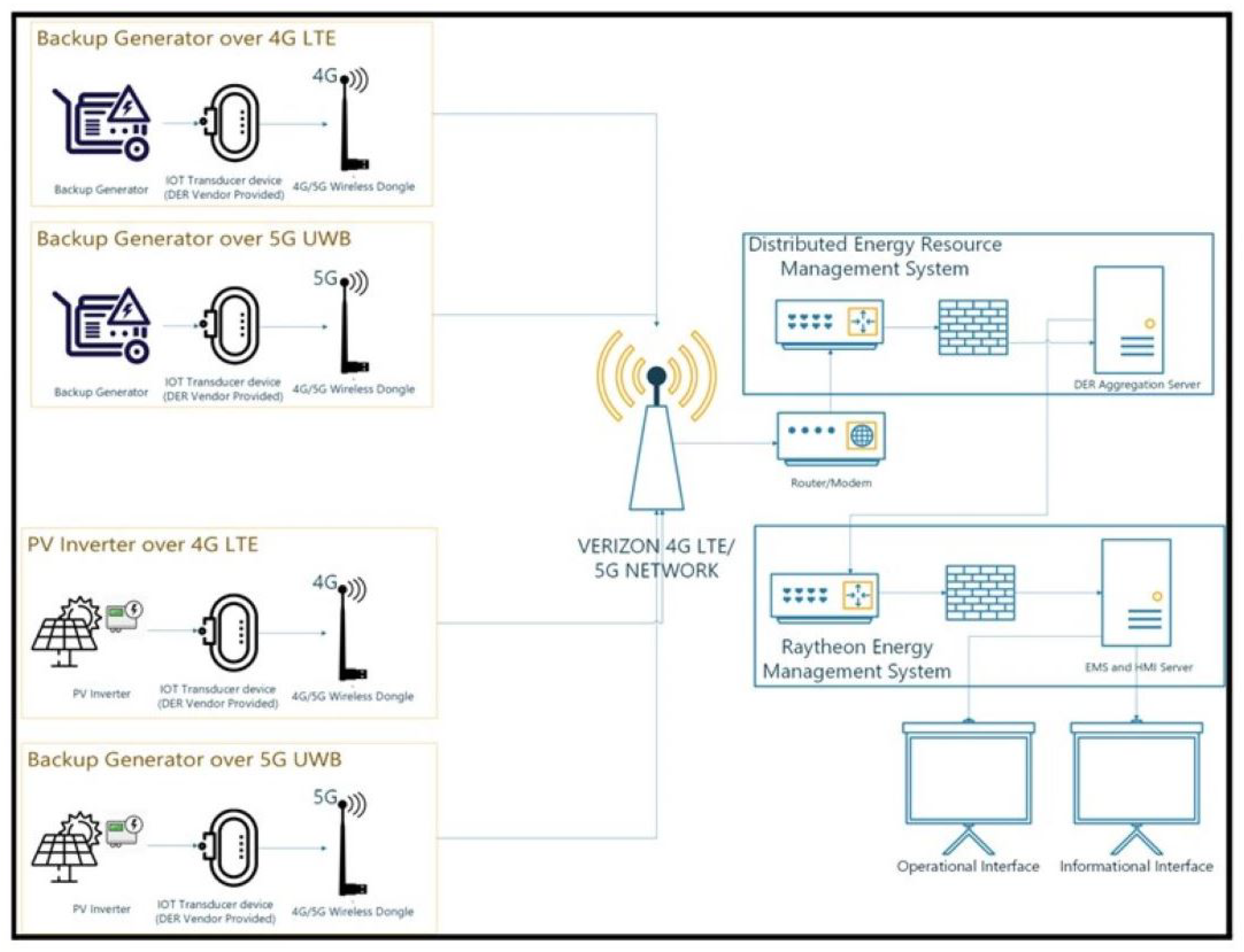
Figure 1 provides a suggested architecture (from US Ignite) for EMS integration with PV arrays and back generators over Verizon’s 4G LTE and 5G networks. The pilot project connects four backup generators and four PV arrays to the 5G NSA network, with the aim to scale to all energy resources at MCAS Miramar. Each DER is connected to an IoT transducer device which is then connected to a 4G or 5G dongle which then forwards traffic to the Verizon 4G LTE/5G tower. The 5G integration for the research microgrid is currently underway at Miramar.

1.2. Research Motivations and Objective

Given the confluence of the wired Modbus TCP/IP over Ethernet traffic and the 5G traffic that is expected on the Miramar energy communications network, the cyber-threat landscape becomes increasing wide and vulnerable.

In terms of the 5G NSA network, it inherits all the vulnerabilities of the LTE network. Furthermore, common solutions in stand-alone 5G networks to alleviate cyber-threats, such as machine learning and virtualization, are inherently unavailable in the NSA network.

In addition, security of the smart meters also needs to be considered. One of the key issues with smart meters is the integrity of the power system estimation data that enters/exits the meter. Mechanisms exist that can differentiate between corrupted data and normal data. However, most techniques fail to detect false data injection attacks (FDIA) [9]. An FDIA is malicious activity designed to manipulate data values.

In this paper, our objective is to develop an anomaly detection framework for the smart microgrid energy infrastructure at Miramar to enhance its cyber-resilience. We implement cyber-analytics using an autoencoder neural network to classify cyber-uncertainties and threats within the microgrid environment. Both network traffic in the form of packet captures (PCAP) (from the 5G and EMS infrastructure) and time series data (from the AMI smart sensors) are used for training and analysis.

1.3. Research Contributions

Our contributions in this work are three-fold:

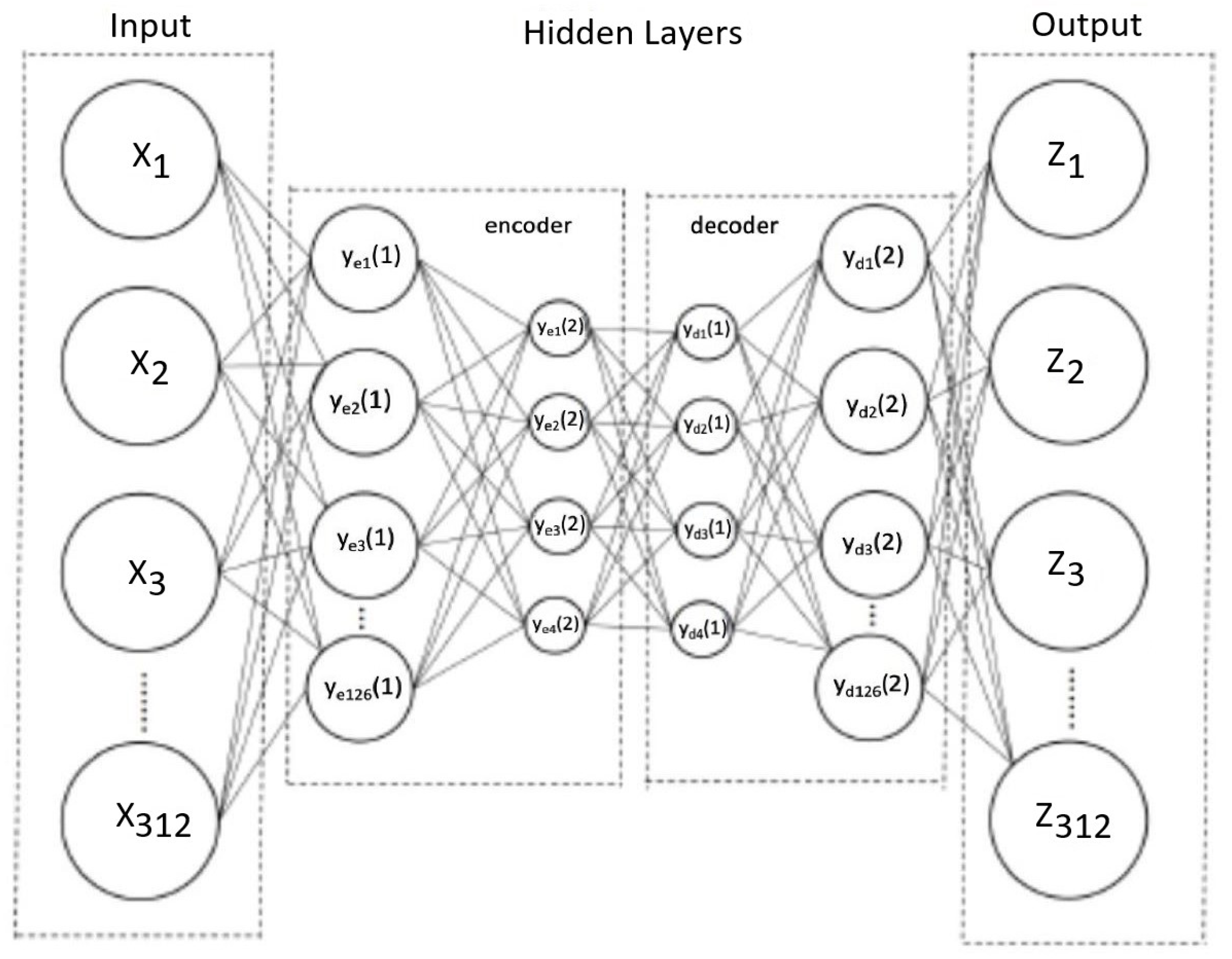
• Model an autoencoder to detect distributed denial-of-service (DDoS) attacks on experimentally generated 5G data, meant to resemble traffic that would be seen on the Miramar 5G wireless network. Given that 5G data on the Miramar energy communications network were not available at the time of this research, we experimentally generated 5G data PCAPs using the AT&T 5G node/infrastructure established on the Naval Postgraduate School (NPS) campus. For the remainder of this paper, we refer to this model as the Efficient autoencoder model. The Efficient model is agnostic to different data sets.
• Train the Efficient model on data from the hardwired EMS network apparatus of the energy communication infrastructure. These data are in the form of Modbus TCP/IP over Ethernet PCAPs and were taken directly from the Miramar network.
• Use the Efficient model to detect FDIA anomalies in the sensor data originating within the AMI smart meter sensors. A time series AMI data set obtained from Naval Facilities (NAVFAC) Engineering Systems Command is used for training.

We quantify model performance using metrics of precision, accuracy, and F2 scores. Python and TensorFlow are used for model implementation and analysis. We also provide a comparison between the Efficient model and that of a deeper model to show how autoencoder complexity affects predictive cyber-analytics.

1.4. Paper Organization

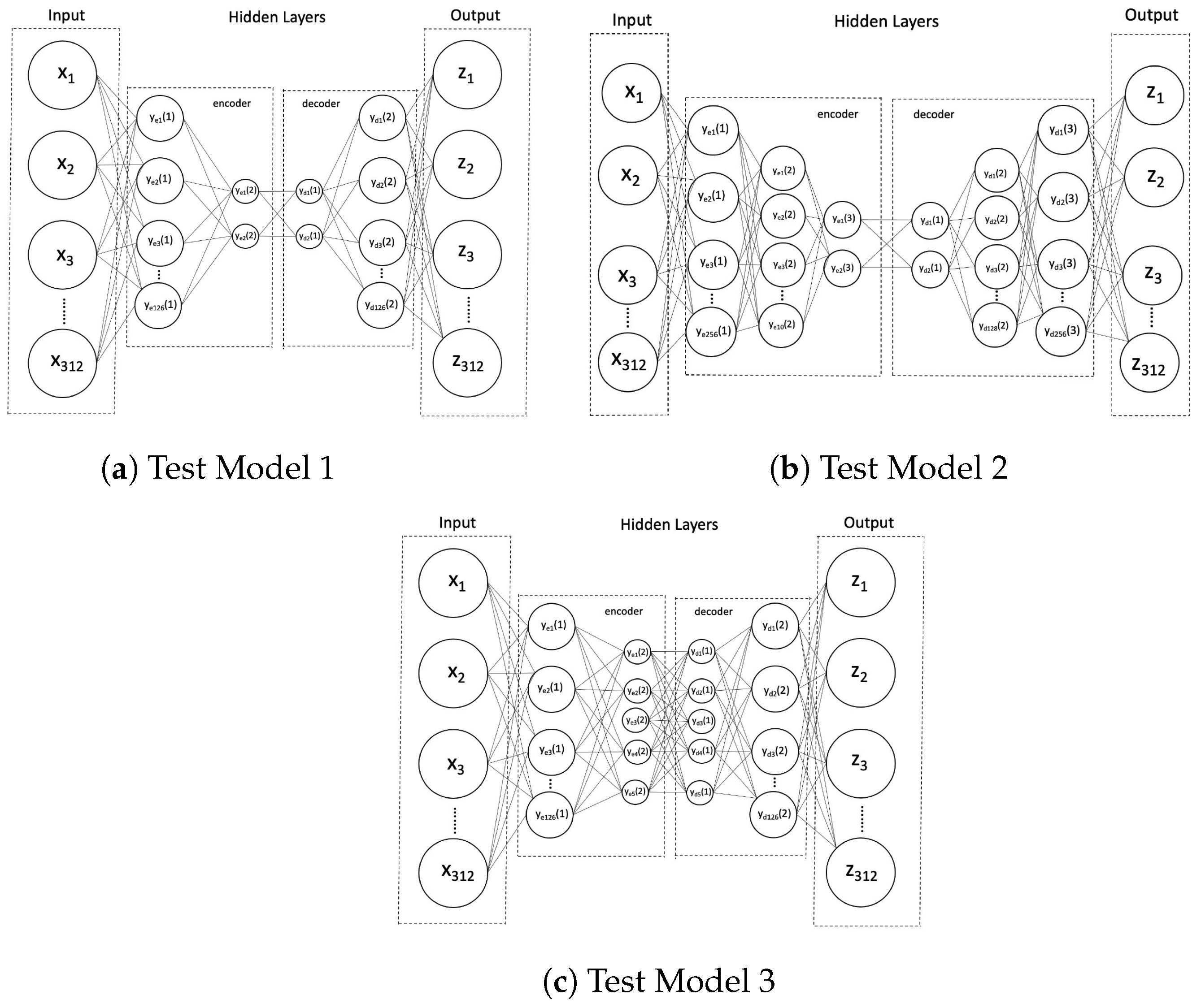
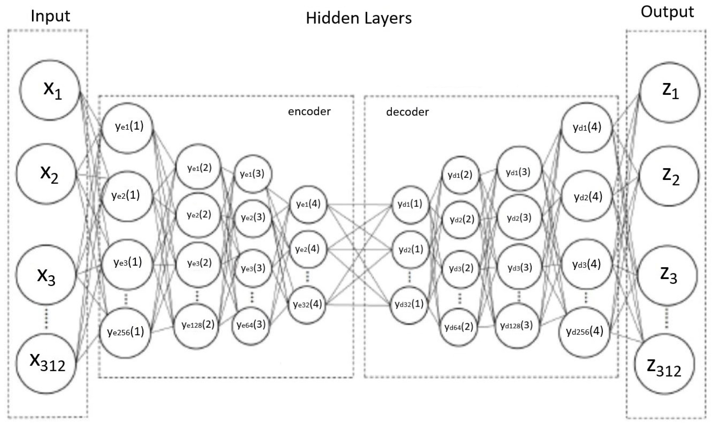
The remainder of this paper is organized as follows: Section 2 covers related work. Section 3 presents our methodology for data gathering, processing, and feature selection. Section 4 discusses the AMI time series data and how they were processed to insert varying degrees of FDIAs. Section 5 discusses the Efficient autoencoder model and the different configurations used for testing. We also discuss the Deep model that is used for comparison. Section 6 presents our approach to synthetic DDoS anomaly generation and the results of our experiments. Finally, Section 7 concludes our work.

2. Background and Related Work

Machine learning has been used extensively in the literature to study network traffic anomalies for critical infrastructure. In [10], the authors provide a comprehensive view of machine learning strategies for anomaly detection in 5G networks, with an emphasis on convolutional neural networks (CNNs). In [11,12], the authors use labeled, open-source Modbus data sets to train for anomalies on data sets representing SCADA systems. Bayesian classification is used in [12] and the K-nearest neighbor algorithm is used in [11]. Despite adequate classification results, both researchers note the limitation of their data sets and the difficulty of acquiring labeled real-world data. Similarly, autoencoders have been used for anomaly detection in IoT based ICS [13]. In their paper, the authors of [13] provide an autoencoder model for intrusion detection in an industrial IoT system, using a real-world ICS data set.

Unlike the work discussed above, our research utilizes real world PCAP data procured from Naval infrastructure to enhance cyber-anomaly detection using ML strategies.

In addition to choosing an anomaly detection model, it is also important to accurately study how to represent network traffic. Through our literature survey, we determined that Yang et al.’s 2020 study [14] was most comprehensive in outlining how to represent and partition data for anomaly detection. In their paper, the authors of [14] proposed various feature representations and machine learning models that were tested and compared for general novelty detection in network traffic, including an autoencoder [14]. Guidelines are provided for selecting features that are most appropriate for different scenarios [14]. Many situations must be considered by network operators when designing an anomaly detection system, such as attacks, malware, new devices or applications, and unusual changes in network traffic [14]. Therefore, selecting a proper data representation is as important as selecting a good model [14].

Yang et al. partitioned packet capture (PCAP) files into forward flows using a five-tuple identifier (source IP, source port, destination IP, destination port, and IP protocol) [14]. However, these identifiers do not appear in the feature vectors. Features that are too specific (IP addresses, port numbers, sequence numbers, etc.) are excluded so that learning can be generalized and not associated with a “specific source, destination, application, or location in the network” [14]. To increase the number of samples, forward flows are sub-partitioned into small time intervals, referred to as subflows [15]. Although the data sources and testing approach in this paper differ significantly from those used by Yang et al., our work is based primarily on lessons learned from this study.

Separate from, but integral to, the microgrid energy assets is the AMI and specifically the smart meters/sensors that it is comprised of. In a smart microgrid, smart sensors collect data from the physical environment. Examples of smart sensors include electric current sensors and voltage sensors. The data collected and transmitted from these smart sensors are open to manipulation, either through benign means (faulty sensors) or malicious means (cyber-actors).

Data drift is one type of benign way in which sensors can produce irregular data due to natural device faults. In [16], the authors study drift detection algorithms for IoT sensors in an industrial control system (ICS). A double linear regression method is used to model predictive behavior.

In [17], the authors detail the process by which faults can be identified in data sets originating at sensor nodes. To facilitate a systematic exploration of sensor anomaly detection, the authors suggest using injected faults as a first step to evaluate detection models. By artificially injecting faults of varying intensity into sensor data, we can quantify the performance of the anomaly/fault detection model. FDIAs are commonly used in power systems to detect abnormalities in power measurements [18,19,20,21].

Autoencoders have also been used to develop intrusion detection system (IDS) methods for power grids and smart power grids. The authors of [22] introduced an unsupervised machine learning approach to anomaly detection using an IEEE 118-bus system data set. The researchers developed an autoencoder to detect false data injection attacks (FDIAs) using an hourly power load data set from 32 European countries. The data set used consisted of macro-level power generation parameters (total power generation, total power consumption, installed capacity, price, etc.) rather than power analysis within a specific smart grid. Unlike [22], we train our autoencoder on a time series data set that includes specific power statistics of each AMI sensor. The model in [22] is used as a comparative architecture to the autoencoder built in this paper. We refer to the model in [22] as the Deep model.

Basics of Autoencoders

An autoencoder is a neural network designed for representation learning by using a hidden layer (or “bottleneck”) in the network, forcing a compressed knowledge representation of the original input [23]. To achieve representative learning, autoencoders apply backpropagation, setting the target values equal to the inputs. By defining the desired output as the input values, an autoencoder can train without using labeled data.

A basic autoencoder includes an encoder, bottleneck, and decoder. The encoder compresses the input data into a latent space representation, reducing the dimensionality and distorting the original data. The bottleneck represents the compressed input, retaining only relevant information from the input [24]. The decoder decompresses the data back to the original dimension. The data are reconstructed from the latent space representation, which produces a lossy reconstruction of the original data [24].

To explain the learning process, consider an autoencoder with only an input and output layer. The learning process is defined by:

$$h=\sigma (W_{x_h}x+b_{x_h})$$

(1)

$$z=\sigma (W_{h_x}h+b_{h_x})$$

(2)

where x is the original input vector (ground truth), z is the reconstructed vector (the model’s prediction), $\sigma$ is the nonlinear activation function, b is the bias, and W is the weight of the neural network [25]. The autoencoder uses an activation function to transform the input vector x into a hidden representation h [25].

After the input vector is compressed into a hidden representation, we calculate the reconstruction error or loss function. For this research, we use the mean squared error (MSE) regression model. The MSE is given by

$$r=\frac{1}{N}\sum _{i=1}^N{(x_i-z_i)}^2$$

(3)

where N is the number of data points in the data set, and the difference between vector z and vector x is squared. The average is then taken across the entire training set.

To find the delta $\delta$ after calculating the reconstruction error, we use

$$\delta ={\sigma }^{\prime }\left(x_i\right)r_i$$

(4)

where $\sigma$’ is the derivative of the activation function. For an autoencoder with multiple hidden layers, the delta is calculated at each layer and updated accordingly.

After the input layer, the remaining layers use an activation function to transform the weighted sum of the inputs into an output. After the activation function is applied to the last layer of the encoder, the values transfer to an optimizer to minimize training loss and improve training accuracy.

3. 5G and Modbus Datasets

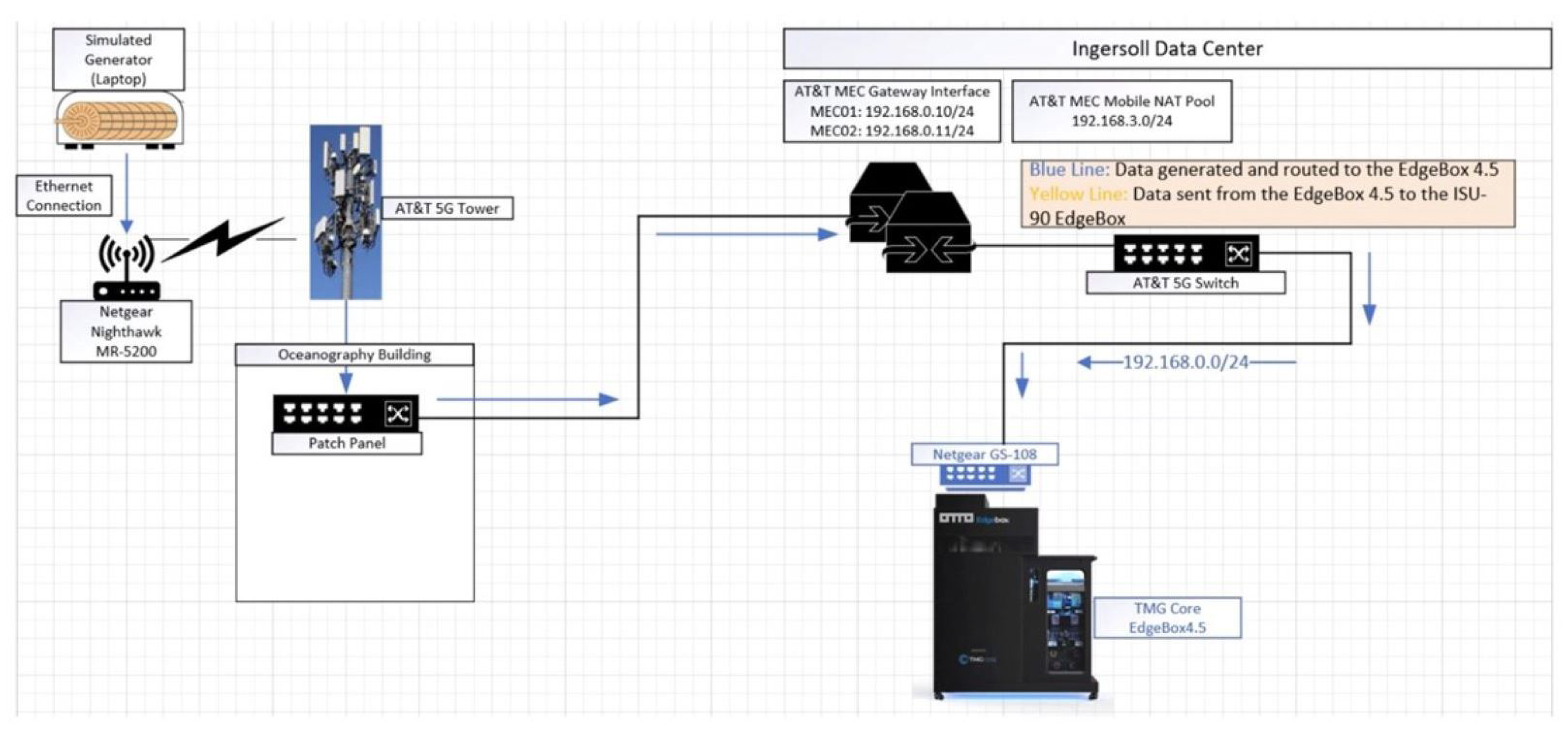
Pending wireless integration of the DER with the existing EMS at Miramar, 5G data traffic was experimentally generated using AT&T’s 5G cellular tower at the NPS Sea Land Air Military Research (SLAMR) facility [8]. The purpose of capturing this traffic was to prepare for the type of traffic flows that may be observed in the newly integrated system. To capture 5G network traffic, a Linux laptop was directly connected via Ethernet to a NetGear Nighthawk M5 5G (MR5200) mobile router [8]. The M5 was configured to run the wireless gateway from the cellular tower to the TMGCore EdgeBox 4.5 located on the NPS campus [8]. The EdgeBox functions as a high-performance data center [26] and is connected to the 5G network at NPS using AT&T’s multi-access edge compute (MEC) nodes [27]. Three open-source PCAP files were replayed over the 5G network: normal traffic [28], Modbus ICS traffic with various cyber-attacks/anomalies [29], and Building Automation and Control Network (BACNET) traffic [30]. The rsync command was executed on the Linux laptop to transfer multiple files to the EdgeBox, and the tshark utility was used to capture the inbound network traffic [8]. Figure 2 shows the experimental data path from the Nighthawk to the EdgeBox. This is the data path used for data collection. The simulated generator, labeled on the upper left of Figure 2, represents the Linux OS laptop that stored the three files that were replayed.

In addition to our experimentally generated 5G data, Raytheon provided Modbus TCP/IP over Ethernet PCAPs taken directly from the existing EMS at Miramar. This preliminary network data were intended to give us insight into the nature of network flows expected from the completed system. Although these data were captured on the wired side of the EMS, we expect similar network traffic flows from the DER to the EWOC facility over the mobile network, with the primary exception being network speeds. The data set contained 15,135 packets. The range of packet sizes were between 40 bytes and 1280 bytes. The average packet size was 121 bytes. This traffic was captured between the EMS and three different DERs.

3.1. Process Flow

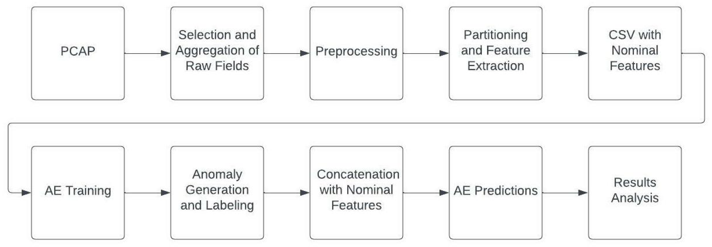
To test the feasibility of the Efficient model for anomaly detection, PCAPs from both AT&T’s 5G network and the wired EMS Modbus network were partitioned and statistics regarding data rates, packet sizes, and packet headers were extracted from the groups of packets. These statistical feature vectors were then used to train our autoencoder models for detection of anomalous flows in network traffic. Synthetic flood statistics (representing a botnet-based ICMP DDoS attack) were generated to test the ability of our models to correctly predict anomalies. Figure 3 shows the process flow diagram which outlines the steps on PCAP processing, feature extraction, and autoencoder training/testing.

The objective of this preliminary process was to obtain a sufficient number of samples, capture the general behavior of the network traffic, and determine which autoencoder model(s) most accurately classified our synthetic anomalies.

3.2. Pcap Processing

We began by processing multiple 5G PCAPs obtained from the AT&T experiment. First, a tshark shell script was written to extract the necessary raw fields from each file. Once that had been completed, the data were concatenated into a single CSV file. The combined CSV file was then loaded into a Python script and the data were partitioned into “flows” as related studies had shown. We refer to this Python script as the extractor because it extracts statistical features after partitioning the data. The extractor’s functionality is implemented using the Pandas library, an open-source data analysis and manipulation tool [31]. All Python scripts written for this work can be found on Github at the links given in [32,33].

3.3. Partitioning

While Yang et al. [14] used a five-tuple identifier for flow partitioning, we believe that ignoring the source would better detect DDoS attacks. A DDoS attack floods a target node/destination node with traffic, thereby exhausting the target node’s resources and denying their service to other network members. A target/destination node can be targeted by multiple source nodes. Our focus in this paper is to use an autoencoder to detect that a DDoS attack has occurred, not to identify who has launched the attack (source or sources). Destination-based DDoS monitoring has been used in the literature [34,35]. Therefore, we opted to use the three-tuple identifier (IP Dst, Dst Port, IP Protocol). We define these as inward flows. Flows are linked to an identifier using a dictionary. At this point, the flows are further partitioned into subflows using one of two methods: fixed time intervals or a timeout period (inter-arrival time). Partitioning the longer flows into smaller groups greatly increases the number of samples and better captures the instantaneous behavior of network traffic. This is useful because a live system will only analyze small slices of network traffic at a time. We arbitrarily selected 10 s and 2 s for the fixed time and timeout intervals, respectively.

3.4. Feature Selection

Although several data representations were experimented with by Yang et al., we felt most comfortable with the statistical representation of network flows as a starting point. Ten statistical features were originally selected: subflow duration, packets/s, bytes/s, and packet size information (mean, std, q1, q2, q3, min, max) [14]. We dropped subflow duration because we believe if the autoencoder is trained to associate statistics with specific durations, more false positives will occur. A real-time system should verify that current network statistics are within nominal range, independent of analysis duration. We also converted bytes/s to bits/s (Mbps or kbps) as this is a more standard representation of network data rates.

3.5. Miramar EMS Modbus Data

A similar process was executed on the Miramar EMS data as the 5G PCAPs. Both timeout and fixed interval sub-partitioning methods were explored. We observed that setting the timeout interval too high resulted in unbroken flows, and setting it too low resulted in many subflows with very brief durations. We then compared the results with the fixed interval method. After some initial testing, we determined that setting the fixed interval to 5 s best captured the behavior of the Modbus network traffic and resulted in fewer subflows with brief durations. The timeout interval remains 2 s.

4. AMI Time Series Data Set

We obtained an AMI time series data set from the Naval Facilities (NAVFAC) Engineering Systems Command, which also oversees some of the Miramar energy network.

The data set received from NAVFAC is similar to that of the Miramar AMI and their results are comparable. The data set includes 35 metering statistics (power, current, voltage, phase, frequency, etc.) from 1200+ AMI devices. The system recorded meter readings once an hour every day from the beginning of January 2020 to the end of January 2021, equating to 9528 inputs per meter statistic.

NAVFAC provided 13 time series data sets as .xml files. Each data set represents the month the data were collected. The data were formatted such that the first column identified the device and the meter statistic. The corresponding row values were the readings taken every hour that month. We removed the timestamp, which was irrelevant for our experiments, and formatted each column to correspond to a meter statistic.

After dropping the time series data, we removed all input features that were not statistical values (‘yes’/‘no’ entries). This reduction compressed our feature input space from 35 inputs to 26 per AMI (as shown in

Table 1. The list of the 26 NAVFAC data input features (per AMI) used for training the autoencoder model.

1	Phase A Current
2	Phase B Current
3	Phase C Current
4	Neutral Current
5	Meter Frequency
6	Average kVAR
7	Average kiloWatts
8	Instantaneous kW
9	Maximum kVAR
10	Maximum kW
11	Phase A-B Voltage Phase Angle
12	Phase A Current Phase Angle
13	Phase A Voltage Phase Angle
14	Phase B-C Voltage Phase Angle
15	Phase B Current Phase Angle
16	Phase B Voltage Phase Angle
17	Phase C-A Voltage Phase Angle
18	Phase C Current Phase Angle
19	Phase C Voltage Phase Angle
20	Phase A Current THD
21	Phase A Voltage
22	Phase A-B Voltage
23	Phase B Voltage
24	Phase B-C Voltage
25	Phase C Voltage
26	Phase C-A Voltage

).

From there, we converted all input values that had error readings (such as ‘I/O Timeout’ or ‘No Data’) to the average of its corresponding column. We converted approximately 16% of the data due to error readings. Following the data manipulation, we concatenated the 13 .xml files into one file.

Fdia Insertion

Once the data set was in one file, our last step was the insertion of an FDIA. To simulate an FDIA, we increased 10% of the data by a certain percentage, mimicking the research performed in [22]. For this research, we performed two types of FDIA. The first attack selected all input values and increased them from 1–10%, incrementing by one. The range started at 1% to find the smallest percent increase that was detectable with acceptable results. It ended at 10% because our experiments showed that the performance plateaued at this upper threshold value. The second attack increased all voltage, current, and power values using the power equation defined by

$$P=VI$$

(5)

where V is voltage and I is current. This attack changed roughly 40% of the input features. The voltage and current values were increased from 2–5%, incrementing by one, with the power values corresponding to Equation (5). The percent increase for the second attack started at 2% because a 1% increase would have negligible effect on the power values. Furthermore, the percent increase for voltage and current stopped at 5% because the corresponding power change in that scenario is a 25% increase. We determined that a power increase above 25% would no longer constitute a nuanced FDIA.

To separate the data between normal and anomalous activity, we added a ‘Malicious’ column to the spreadsheet. For this column, we define 1 and 0 to represent ‘Malicious’ and ‘Normal’, respectively. Therefore, for the ten percent of data whose values were increased to mimic an FDIA, a 1 was placed in the “Malicious” column. The remainder of the data received a 0 in that column.

5. Model Configurations

Our Efficient anomaly detection model is placed at the data concentrator (located in the EWOC) which receives the data from the AMI sensors. For the 5G and EMS data, the model is placed at the point of presence (PoP) between the 5G NSA network and the EMS Modbus data network.

5.1. Activation Finctions

In our experiments, we used three activation functions:

• ReLU + Linear—The ReLU (rectified linear unit) activation function maps negative inputs to zero and acts as an identity function for non-negative input [36]. The output layer uses a linear activation function so that output values will be unbounded.
• LeakyReLU—With LeakyReLU activation, negative inputs are not mapped to zero but are still very small. Traditional ReLU can lead to the “dying ReLU” problem in which all inputs to a node are mapped to zero, slowing down the learning process [36]. This activation function is the default used by Yang et al. [15].
• Sigmoid—Sigmoid activation is a common activation function used for shallow neural networks. It is called a logistic function because it outputs values between zero and one. However, Sigmoid suffers from the vanishing gradient phenomenon, which restricts the contributions of the first several layers to the learning process during training. We use this activation function to compare with the Deep model [22] which uses Sigmoid and ReLu.

5.2. Optimizers

For our experiments, we used three different optimizers:

• Adaptive Moment Estimation (Adam)—Adam is a popular optimization algorithm for gradient descent. Adam uses a combination of adaptive gradient algorithm (AdaGrad) and root mean square propagation (RMSProp), which are both adaptive learning algorithms [37]. This contrasts with traditional gradient descent algorithms that maintain a fixed learning rate during training.
• Lookahead—The Lookahead optimizer attempts to improve gradient descent algorithms. It takes another optimizer as input and manipulates it to enhance its performance [38]. We experimented with Adam enhanced with Lookahead to see if there was any meaningful improvement.
• Stochastic Gradient Descent (SGD)—The network parameters are updated as the optimizer processes each mini-batch of training data as opposed to adjusting after the entire training data set has been evaluated. Adam is a follow-on to SGD. We use SGD to accurately compare with ref. [22]’s work.

5.3. Efficient Autoencoder Model: Testing and Structure

To establish a baseline for this research, several autoencoders were built and tested. Before training and testing the models on the various data sets used in this paper, the autoencoders were tested on an open-source Modbus data set to determine the best performing model. The Modbus data set was generated via an SCADA sandbox, using electrical network simulators [39]. The data included six separate data sets, six with normal network traffic, and five with a mix of malicious and normal traffic. From these data sets, we selected four mixed data sets and additionally created another data set that combined all the data sets with mixed network traffic. Four autoencoder models were built and tested.

Our first experiment was a two-layer autoencoder that compressed the input features by half at the first layer and then to two nodes at the second layer. We refer to this as Test Model 1, and it is shown in Figure 4a. The reasoning behind this structure was to force the autoencoder to make a binary decision—either the input was normal or malicious. However, this autoencoder produced poor results, with very high false positives. The second autoencoder model, Test Model 2, added another layer (Figure 4b). The model compressed the inputs by half, then to ten nodes, and then to two nodes. The rationale for the additional layer was to expand the depth of the model, increasing the number of opportunities to learn the latent space representation while maintaining a binary bottleneck. However, the model failed to improve. Since the second model did not improve from the first, we reverted back to a two-layer structure. As shown in Figure 4c, Test Model 3 kept the same first layer but changed the compression at the bottleneck. Rather than two nodes, like the previous two models, the second layer was compressed to five nodes. This change challenged the assumption that the best autoencoder needed to be compressed to a binary decision space. Test Model 3 performed significantly better than the previous models. From this point, we ran two more tests in which Test Model 4 compressed the second layer to four nodes and Test Model 5 compressed the second layer to three nodes. The performance across Test Models 3, 4, and 5 were similar. However, after numerous tests, Test Model 4 consistently produced slightly better accuracy, recall, and precision scores. Test Model 4 is what we denote as the Efficient Autoencoder Model used in this paper and is shown in Figure 5. The results of all these tests can be found in [40,41].

Efficient Autoencoder Model

The Efficient autoencoder model includes two dense layers of compression and then the reconstruction. The input layer is reduced by half and then compressed to four nodes. From there, the model expands using the same dimensions as the encoding layer back to its original size. We trained the Efficient model on the 5G PCAP data, EMS Modbus PCAP data and NAVFAC AMI time series data sets.

Different combinations of activation functions, optimizers, and PCA principles were applied to the autoencoder. In TensorFlow, we tune certain parameters for our experiments. These parameters are batch size, learning rate, and epochs. The batch size is the number of data samples processed before the model is updated. The learning rate is a tuning parameter in an optimization algorithm (such as Adam, SGD, and Lookahead) that determines the step size at each iteration while moving toward a minimum loss function. Lastly, the number of epochs is the number of complete passes through the training data set. Also, in our model we must guard against overfitting [42]. Overfitting occurs when models learn the specifics of a training data set too well. This causes the model to not be able to generalize to new data sets and is usually due to the limits of training data [42]. The early stop callback function is a common solution to overfitting. It allows us specify an arbitrarily large number of training epochs and stop training once the model performance stops improving on the validation data set.

Our models used a batch size of 128 and a learning rate of 0.01 for the Adam and Lookahead optimizers or 0.001 for the SGD optimizer. The model ran for between 700 and 1500 epochs depending on the data set. We used the early stop callback function to prevent overfitting.

After training on nominal data points, a threshold is determined using standard deviations from the MSE of nominal predictions. Any input vector with a reconstruction error exceeding the established threshold will be classified as anomalous.

5.4. Pca Principles

An autoencoder model that improves the test reconstruction error retains the following PCA principles: tied weights, orthogonal weights, uncorrelated features, and unit norm weights [43]. We chose to incorporate some of these principles into our autoencoder, effectively extending them into nonlinear space [43]. Specifically, we experimented with tied weights and unit norm constraints to see if they had any effect on tuning and optimization. Tied weights and unit norm weights act as a type of regularization. Orthogonality and uncorrelated features constraints were not explored in our study.

5.5. Deep Model

The Deep model autoencoder was developed in [22] and is used for comparison against the Efficient model discussed in Section 5.3. The Deep model autoencoder includes four dense layers of compression and decompression, as described in [22]. Figure 6 illustrates the deep model’s architecture. We chose the autoencoder in [22] because it proved effective at detecting anomalous activity on a traditional power grid data set and its structure is deeper than the Efficient model generated in this paper.

5.6. Training

The following optimizers and activation functions were used for each of the data sets.

• 5G and EMS PCAP data set trained using our Efficient autoencoder model:

  –

  Activation functions: Relu and LeakyRelu;

  –

  Optimizers: Adam and Lookahead.

• 5G and EMS PCAP data set trained using Deep autoencoder model of [22]:

  –

  Activation functions: Relu and LeakyRelu;

  –

  Optimizers: Adam and Lookahead.

The activation functions and optimizers for the PCAP data sets were chosen based on the parameters used in Yang’s paper.

• AMI sensor data set trained using our Efficient autoencoder model:

  –

  Activation functions: Relu and Sigmoid;

  –

  Optimizers: Adam and SGD.

• AMI sensor data set trained using Deep autoencoder model of [22]:

  –

  Activation functions: Relu and Sigmoid;

  –

  Optimizers: Adam and SGD.

The activation functions and optimizers for the time series AMI data sets were chosen based on the parameters used in [22].

6. Testing and Results

6.1. Anomaly Generation for 5G Data Set

Due to the lack of real-world microgrid attack data, we needed to determine a method to obtain anomalous flows to test the autoencoder models. To simulate an anomalous traffic flow, network statistics outside nominal range must be generated. To accomplish this, a Python function takes as input a packet size and number of packets/s and returns a statistical feature vector representing a botnet-based ICMP flood with equal-sized packets. Several of these synthetic flows were generated, each with different data rates to show that stronger DDoS attacks result in larger reconstruction errors. This function works by fixing the packets per second and increasing the packet sizes for each iteration.

6.2. Experiment Setup

Synthetic flows were generated for both 5G and Modbus data sets. Lower bounds were deliberately set to be outside nominal range, and upper bounds were arbitrarily selected for clear visualization.

• 5G Nominal (average): 21.7 mbit/s (@1300 packets/s).
• 5G Anomalies: 24 mbit/s—120 mbit/s (@3000 packets/s).
• Modbus Nominal (average): 5.93 kbit/s (@9.19 packets/s).
• Modbus Anomalies: 10.24 kbit/sec—80 kbit/s (@20 packets/s).

Although the data rates by themselves are not unusual, the abnormal packet size statistics significantly increase the reconstruction errors. After attaching the synthetic flows to their respective nominal data frames, each saved autoencoder model was loaded and predictions were made.

6.3. Performance Metrics

Accuracy is the ratio of correct predictions over the entire data set [44]. Recall is the ratio of the total true positive values ($t_p$) predicted to the sum of true positive values and the total number of false negative numbers ($f_n$) [45]. Recall is given by

$$Recall=\frac{t_p}{t_p+f_n}$$

(6)

where the ratio of the total true positive values ($t_p$) predicted to the sum of true positive values and the total number of false negative numbers ($f_n$). A perfect recall score of 1.0 indicates that 100% of synthetic anomalies were correctly identified by the model. Precision is the ratio of correctly predicted anomalies to the total number of positive predictions [45]. A precise model indicates a low number of false positives.

Precision is the same as recall but uses the total number of false positive values ($f_p$) rather than false negatives. Precision is defined by

$$Precision=\frac{t_p}{t_p+f_p}$$

(7)

For anomaly detection, operators prefer an increased number of false positives (normal activity labeled malicious) over false negatives (malicious data labeled normal). However, the model should not overtax an operator or system with excessive false alarms.

The F-score (or F-measure) is a useful metric when false negatives are more impactful than false positives (or vice versa) but both are important [45]. While the F1 score provides a weighted average of recall and precision [44], the beta value can be adjusted to emphasize one over the other [45]. Setting the beta value to 2 (F2 score) favors recall over precision, allowing us to select a model that limits false negatives while also maintaining a low false-positive rate.

Threshold

The threshold we used is the same as that of [39]. We used [39] to determine the structure of the Efficient autoencoder model, (Section 5.3), and therefore it made sense to use their same threshold. The detection threshold is set at two standard deviations from the nominal MSE.

Using a similar process to [39], we used the MSE equation given in Equation (3), as the loss function to calculate the reconstruction error. After the model calculates the MSE, the scores are rank ordered. Next, we determined whether the MSE values are two standard deviations or greater from the average. If so, we removed those values. The process of removing the tail values in the distribution curve accounts for any strange but still normal data that entered the model. If we used the highest reconstruction error without removing the outliers, we might set an artificially high threshold, degrading the model’s performance. Once the tail values are removed, the MSE scores within two standard deviations are rank ordered with the maximum value (the highest reconstruction error within the set) established as the threshold [39]. The autoencoder labels the input values with reconstruction errors above the threshold as ‘malicious’ and values below the threshold as ‘normal’.

6.4. Results for 5G and Modbus PCAPS Using Efficient Model

Sixteen autoencoder models were tested and trained on each of the 5G and Modbus TCP/IP data sets. Each model used different combinations of activation functions, optimizers, and weights. After running the prepared data sets through each of the 16 models, the best configurations were selected based on the chosen metrics. Ultimately, we determined that the most efficient 5G configuration used LeakyReLU activations with Adam optimizer and incorporated both tied weights and a unit norm constraint.

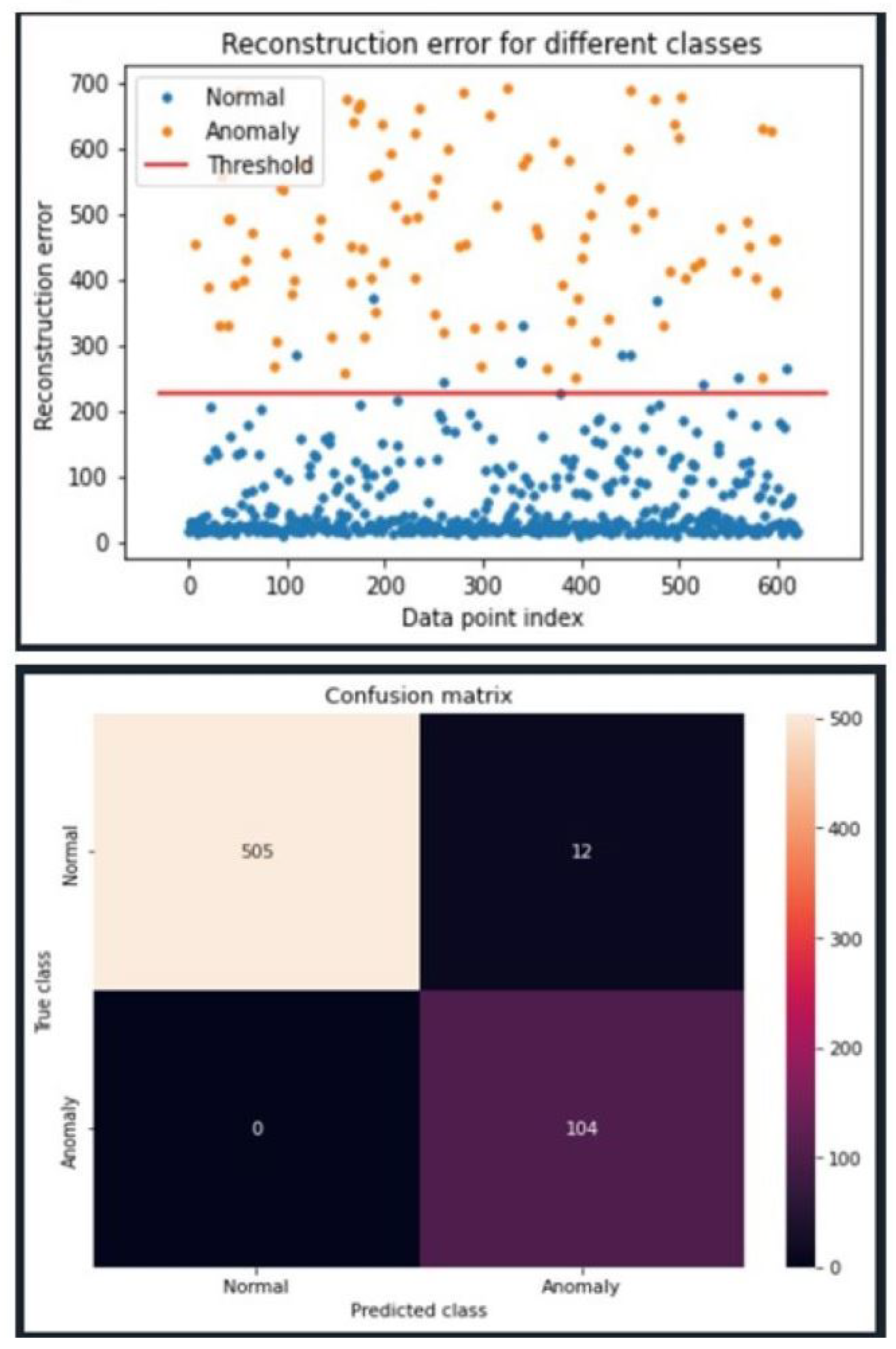
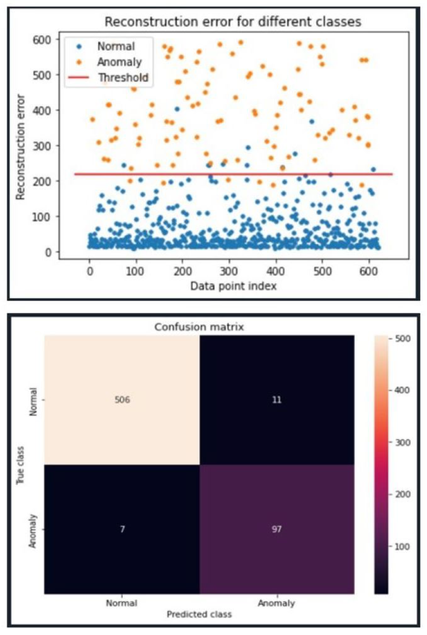
Figure 7 visualizes the detection results for our selected 5G model. The line divides the graph into two sections and is the established threshold. Any error values above the threshold are predicted ‘malicious’, while everything below the threshold is predicted ‘normal’. Orange and blue circles represent malicious and normal data, respectively. Blue circles plotted above the threshold are false positives, while orange circles below the threshold are false negatives. The orange dots, representing anomalous data points, are well above the established threshold. This is reflected by a perfect recall score. The F2 score is 97.5%, indicating the model also has a low false-positive rate. The bottom table reflects a confusion matrix and shows the total number of true positives (top left), false positives (top right), false negatives (bottom left), and true negatives (bottom right) for the same data set used to generate the top figure. From the bottom figure, we see 505 true positives, 12 false positives, 0 false negatives, and 104 true negatives. This results in a 98% accuracy. The remaining results for the other 15 model configurations for the 5G data set can be found in [46].

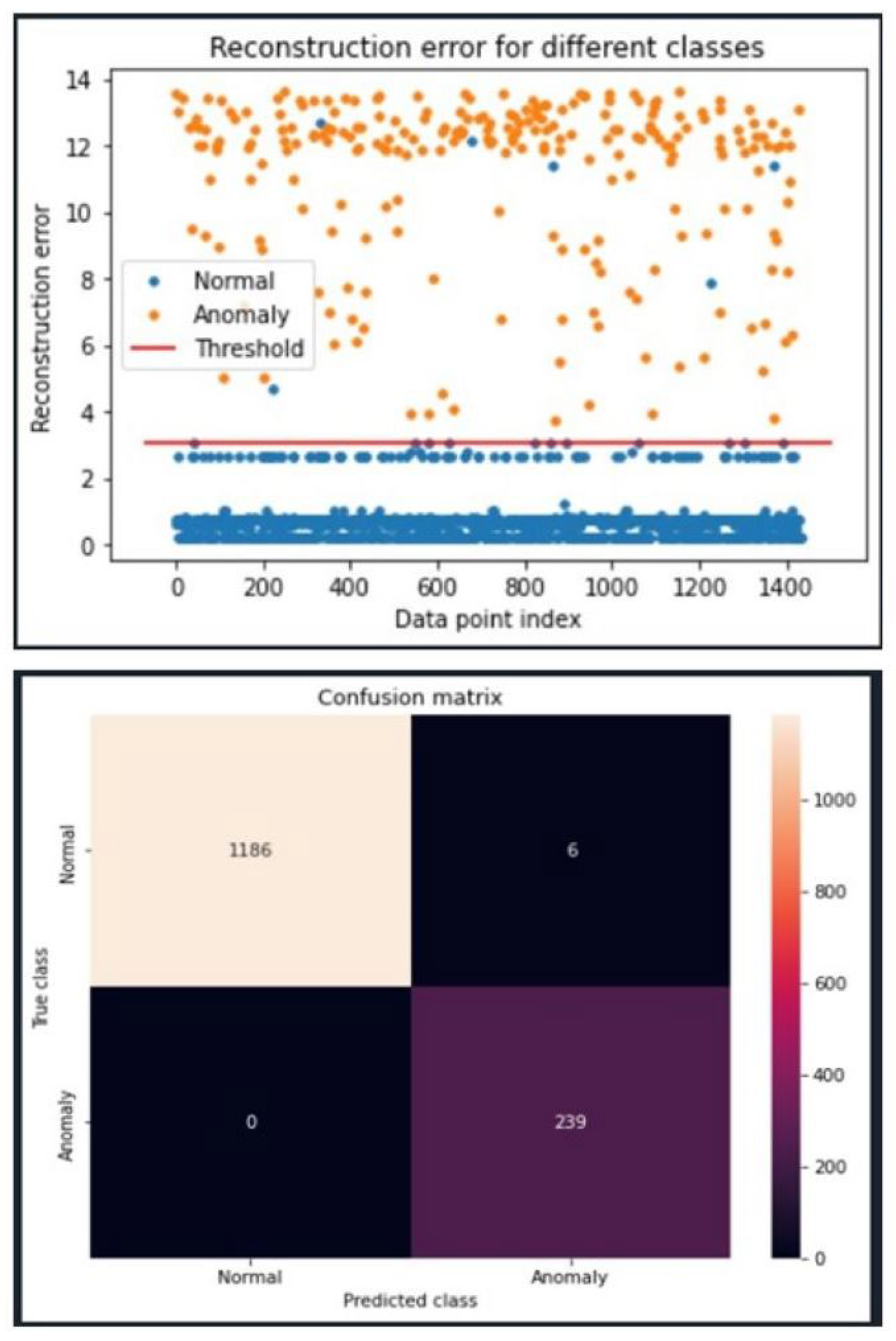
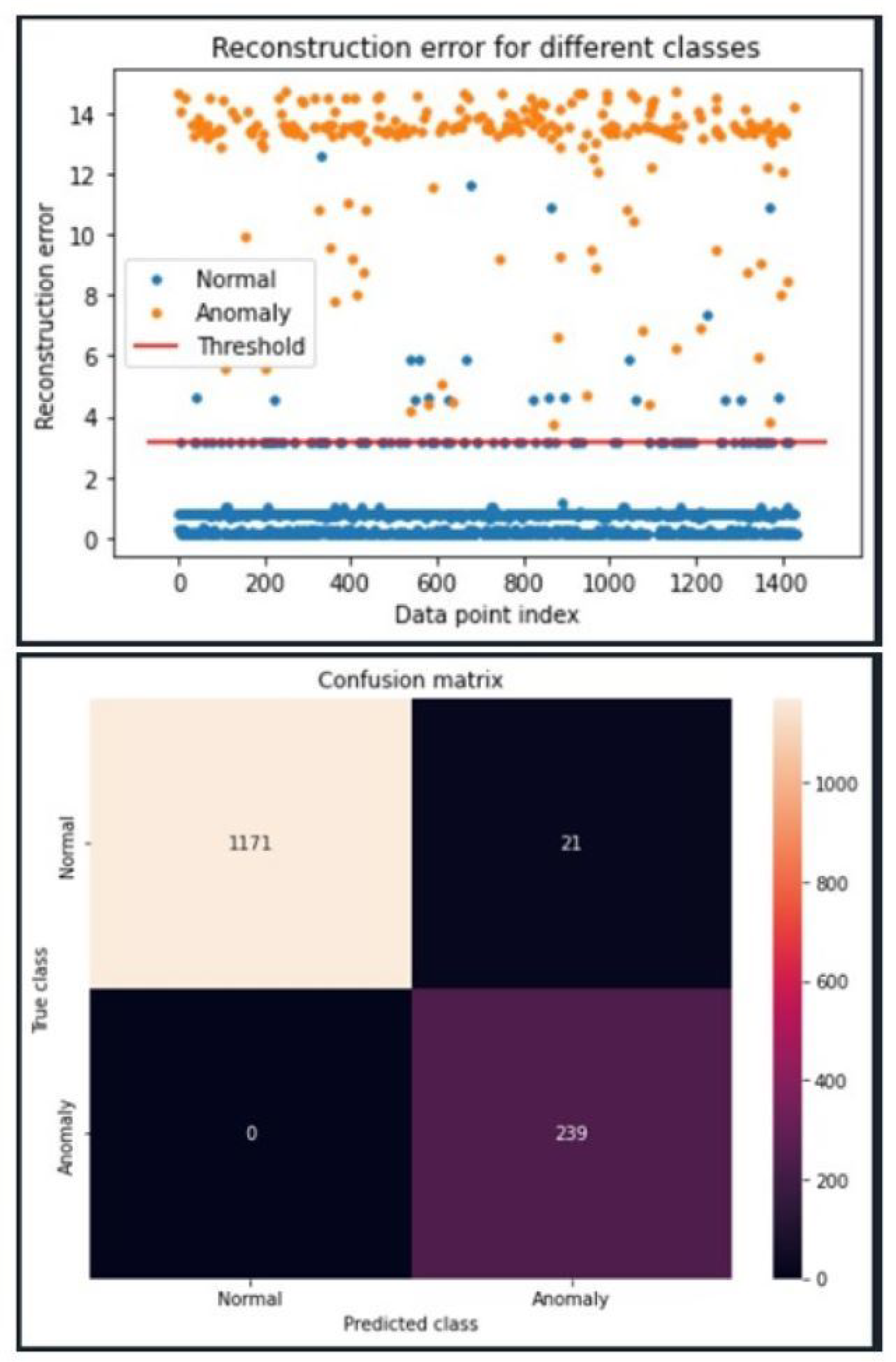
Many model configurations performed equally well on the Modbus data, including the 5G model configuration depicted in Figure 7. For this reason, we opted to select the same configuration for the Modbus model. Figure 8 illustrates that with this configuration, all synthetic anomalies are significantly above the established threshold and perfect recall is achieved. A near-perfect F2 score of 99.5% is observed due to the extremely low false positive rate. In this case, 1186 true positives, 6 false positives, 0 false negatives, and 239 true negatives were found. This resuls in a 99% accuracy.

The selected configuration demonstrates the successful effects of incorporating some PCA properties on the base LeakyReLU model’s weights. With this configuration, near-perfect F2 scores are achieved for both the 5G and Modbus data sets. In a real-world system, these results translate to a high detection rate for ICMP flood attacks with few false alarms.

6.5. Results for 5g and Ems Data Sets Using Deep Model

The following are results from when the Deep model was tested using the same activation and optimizer combination as the Efficient model. From Figure 9 we were able to calculate a recall rate of 0.94, an accuracy of 97% and an F2-score of 92%. Similarly, in Figure 10, we see a recall of 1, an accuracy of 98% and an F2 score of 95%.

Due to the deeper number of levels of the Deep model, it converges two to five times slower than the Efficient model. Despite the deeper structure of the Deep model, its performance was very similar or worse than the Efficient model in all tests (5G PCAPS and Modbus TCP/IP PCAPS). Therefore, a more complicated (deeper) model did not facilitate better results on either the 5G data set or the Modbus TCP/IP data set. The Deep model has no significant benefit over the Efficient model, which shows that a simpler, leaner autoencoder structure is highly effective for this use case.

6.6. Results for Navfac AMI Data Set

We created 14 different data sets from the given NAVFAC data set. Ten of the data sets mimic an FDIA across all AMI input parameters, representing a broad attack on the smart grid. As discussed in Section 4, these attacks increase the input values across the AMI data set from 1 to 10%, incrementing by one. In Table 2, Table 3, Table 4 and Table 5, these attacks correspond to the rows with only a single percent in the ‘% Increase’ column (1–10%). The other four data sets simulate an FDIA on specific input parameters—voltage, current, and power. These changes to specific input parameters mimic nuanced attacks. These attacks are displayed in the rows with two distinct percentage values in the ‘% Increase’ column (bottom 4 rows of Table 2, Table 3, Table 4 and Table 5). The first percent value represents the percentage increase to the voltage and current parameters. The second percent value corresponds to the change in the power input parameter using the power equation discussed in Section 4.

6.6.1. Efficient Model–Sigmoid and Adam/SGD

Table 2 displays the Efficient Model’s performance using the sigmoid activation function and the Adam or SGD optimizers. When testing against an FDIA across all AMI input parameters, a 3% increase and above produced impressive results, with only recall failing to score in the mid 90%. However, at the 4% mark and above, accuracy, recall, and precision were all in the mid to high 90%. When simulating an FDIA on specific AMI parameters, current and voltage, the model did not produce positive results until a 4% increase to the voltage and current parameters. At the 2–3% increase for current and voltage, the recall score ranges from the mid-50s to high-60s percentage values. However, at the 4% mark, the Efficient model produces high accuracy and precision, and acceptable recall. With a 5% increase, the model produced mid-to-high 90s percentage values across all these statistics.

Table 2. Results for Efficient Model using Sigmoid activation function and either ADM or SGD optimization on NAVFAC data sets.

Sigmoid
Adam				SGD
% Increase	Accuracy	Recall	Precision	% Increase	Accuracy	Recall	Precision
10%	99.6%	100%	96.6%	10%	99.6	100%	96.6%
9%	99.6%	100%	96.6%	9%	99.6	100%	96.6%
8%	99.6%	100%	96.6%	8%	99.6	100%	96.6%
7%	99.6%	99.7%	96.6%	7%	99.6	99.7%	96.6%
6%	99.6%	99.7%	96.6%	6%	99.6	99.7%	96.6%
5%	99.6%	99.5%	96.6%	5%	99.6	99.5%	96.6%
4%	99.4%	97.6%	96.5%	4%	99.4%	97.4%	96.5%
3%	98.9%	92.9%	96.4%	3%	98.9%	92.6%	96.4%
2%	96.6%	69.2%	95.2%	2%	96.8%	70.7%	95.3%
1%	94.8%	50.0%	93.6%	1%	94.7%	49.8%	93.5%
VI 2%/P 4%	95.1%	54.1%	94.0%	VI 2%/P 4%	95.3%	55.6%	94.1%
VI 3%/P 9%	96.5%	67.7%	95.1%	VI 3%/P 9%	96.5%	68.3%	95.2%
VI 4%/P 16%	98.1%	84.0%	96.0%	VI 4%/P 16%	98.1%	84.0%	96.0%
VI 5%/P 25%	99.0%	94.2%	96.4%	VI 5%/P 25%	99.0%	93.3%	96.4%

Table 2. Results for Efficient Model using Sigmoid activation function and either ADM or SGD optimization on NAVFAC data sets.

Sigmoid
Adam				SGD
% Increase	Accuracy	Recall	Precision	% Increase	Accuracy	Recall	Precision
10%	99.6%	100%	96.6%	10%	99.6	100%	96.6%
9%	99.6%	100%	96.6%	9%	99.6	100%	96.6%
8%	99.6%	100%	96.6%	8%	99.6	100%	96.6%
7%	99.6%	99.7%	96.6%	7%	99.6	99.7%	96.6%
6%	99.6%	99.7%	96.6%	6%	99.6	99.7%	96.6%
5%	99.6%	99.5%	96.6%	5%	99.6	99.5%	96.6%
4%	99.4%	97.6%	96.5%	4%	99.4%	97.4%	96.5%
3%	98.9%	92.9%	96.4%	3%	98.9%	92.6%	96.4%
2%	96.6%	69.2%	95.2%	2%	96.8%	70.7%	95.3%
1%	94.8%	50.0%	93.6%	1%	94.7%	49.8%	93.5%
VI 2%/P 4%	95.1%	54.1%	94.0%	VI 2%/P 4%	95.3%	55.6%	94.1%
VI 3%/P 9%	96.5%	67.7%	95.1%	VI 3%/P 9%	96.5%	68.3%	95.2%
VI 4%/P 16%	98.1%	84.0%	96.0%	VI 4%/P 16%	98.1%	84.0%	96.0%
VI 5%/P 25%	99.0%	94.2%	96.4%	VI 5%/P 25%	99.0%	93.3%	96.4%

6.6.2. Deep Model–Sigmoid and Adam/SGD

Table 3 shows the Deep model’s performance using sigmoid activation and the Adam or SGD optimizers. Similar to the Efficient model, at the 3% increase mark the Deep model produced 98.9% accuracy, 92.9% recall, and 96.4% precision. Additionally, at 4% and above, accuracy, recall, and precision all showed percentages in the mid-to-high 90s. When simulating an FDIA on specific AMI parameters, the Deep model mimicked the Efficient model, failing to achieve positive results until a 4% increase to both parameters. At that point, accuracy and precision scores in the mid-to-high 90s percentage values, and recall scores 84%. At the 5% increase mark, the Deep model produced mid-to-high 90s percentage values for accuracy, recall, and precision (similar to the Efficient model).

Table 3. Results for Deep model using Sigmoid activation function and either ADM or SGD optimization on NAVFAC data sets.

Sigmoid
Adam				SGD
% Increase	Accuracy	Recall	Precision	% Increase	Accuracy	Recall	Precision
10%	99.6%	100%	96.6%	10%	99.6%	100%	96.6%
9%	99.6%	100%	96.6%	9%	99.6%	100%	96.6%
8%	99.6%	100%	99.6%	8%	99.6%	100%	96.6%
7%	99.6%	99.7%	96.6%	7%	99.6%	99.7%	96.6%
6%	99.6%	99.7%	96.6%	6%	99.6%	99.7%	96.6%
5%	99.6%	99.5%	96.6%	5%	99.6%	99.5%	96.6%
4%	99.4%	97.8%	96.6%	4%	99.4%	97.4%	96.5%
3%	98.9%	92.9%	96.4%	3%	98.9%	92.6%	96.4%
2%	96.6%	69.4%	95.2%	2%	96.7%	70.5%	95.3%
1%	94.6%	48.3%	93.3%	1%	94.8%	50.7%	93.6%
VI 2%/P 4%	95.2%	54.8%	94.0%	VI 2%/P 4%	95.2%	55.2%	94.1%
VI 3%/P 9%	96.5%	68.6%	95.2%	VI 3%/P 9%	96.5%	67.7%	95.1%
VI 4%/P 16%	98.1%	84.0%	96.0%	VI 4%/P 16%	98.2%	85.3%	96.1%
VI 5%/P 25%	99.0%	93.3%	96.4%	VI 5%/P 25%	99.0%	93.3%	96.4%

Table 3. Results for Deep model using Sigmoid activation function and either ADM or SGD optimization on NAVFAC data sets.

Sigmoid
Adam				SGD
% Increase	Accuracy	Recall	Precision	% Increase	Accuracy	Recall	Precision
10%	99.6%	100%	96.6%	10%	99.6%	100%	96.6%
9%	99.6%	100%	96.6%	9%	99.6%	100%	96.6%
8%	99.6%	100%	99.6%	8%	99.6%	100%	96.6%
7%	99.6%	99.7%	96.6%	7%	99.6%	99.7%	96.6%
6%	99.6%	99.7%	96.6%	6%	99.6%	99.7%	96.6%
5%	99.6%	99.5%	96.6%	5%	99.6%	99.5%	96.6%
4%	99.4%	97.8%	96.6%	4%	99.4%	97.4%	96.5%
3%	98.9%	92.9%	96.4%	3%	98.9%	92.6%	96.4%
2%	96.6%	69.4%	95.2%	2%	96.7%	70.5%	95.3%
1%	94.6%	48.3%	93.3%	1%	94.8%	50.7%	93.6%
VI 2%/P 4%	95.2%	54.8%	94.0%	VI 2%/P 4%	95.2%	55.2%	94.1%
VI 3%/P 9%	96.5%	68.6%	95.2%	VI 3%/P 9%	96.5%	67.7%	95.1%
VI 4%/P 16%	98.1%	84.0%	96.0%	VI 4%/P 16%	98.2%	85.3%	96.1%
VI 5%/P 25%	99.0%	93.3%	96.4%	VI 5%/P 25%	99.0%	93.3%	96.4%

6.6.3. Efficient Model–Relu and Adam/SGD

Table 4 illustrates the Efficient model’s performance using the ReLU activation function and the Adam or SGD optimizers. As opposed to the results shown in Table 2 and Table 3, the model using ReLU activation performs differently depending on the optimizer. When using the Adam optimizer, performance is consistent. Even with minor increases, the model maintains a far better balance between recall and precision than the other configurations. Recall stays in the mid-to-high 90s percentage values and precision remains in the mid 80s to low 90s, with only a few exceptions. That said, with this structure, the Efficient model produces poor results at the 9% increase and above mark (precision drops to the low 80s percentage values).

Table 4. Results for Efficient model using ReLU activation finction and either ADM or SGD optimization on NAVFAC data sets.

ReLU
Adam				SGD
% Increase	Accuracy	Recall	Precision	% Increase	Accuracy	Recall	Precision
10%	97.7%	98.4%	81.7%	10%	98.9%	100%	90.4%
9%	96.9%	94.1%	78.9%	9%	97.7%	94.1%	84.3%
8%	98.8%	95.4%	92.5%	8%	98.0%	94.6%	86.6%
7%	98.7%	100%	88.9%	7%	99.6%	99.7%	96.4%
6%	97.5%	96.1%	81.8%	6%	98.2%	100%	85.1%
5%	99.0%	100%	91.1%	5%	99.6%	99.5%	96.6%
4%	98.2%	93.7%	88.7%	4%	98.4%	94.6%	90.3%
3%	98.5%	93.1%	89.5%	3%	97.4%	94.8%	81.6%
2%	98.5%	92.4%	93.0%	2%	97.3%	83.8%	88.8%
1%	97.2%	85.0%	86.6%	1%	94.6%	48.3%	93.3%
VI 2%/P 4%	98.8%	98.2%	90.8%	VI 2%/P 4%	97.3%	100%	78.6%
VI 3%/P 9%	97.4%	94.6%	81.9%	VI 3%/P 9%	96.6%	69.2%	95.2%
VI 4%/P 16%	97.5%	92.6%	84.0%	VI 4%/P 16%	98.2%	85.5%	96.1%
VI 5%/P 25%	98.9%	99.7%	90.6%	VI 5%/P 25%	99.0%	99.7%	91.1%

Table 4. Results for Efficient model using ReLU activation finction and either ADM or SGD optimization on NAVFAC data sets.

ReLU
Adam				SGD
% Increase	Accuracy	Recall	Precision	% Increase	Accuracy	Recall	Precision
10%	97.7%	98.4%	81.7%	10%	98.9%	100%	90.4%
9%	96.9%	94.1%	78.9%	9%	97.7%	94.1%	84.3%
8%	98.8%	95.4%	92.5%	8%	98.0%	94.6%	86.6%
7%	98.7%	100%	88.9%	7%	99.6%	99.7%	96.4%
6%	97.5%	96.1%	81.8%	6%	98.2%	100%	85.1%
5%	99.0%	100%	91.1%	5%	99.6%	99.5%	96.6%
4%	98.2%	93.7%	88.7%	4%	98.4%	94.6%	90.3%
3%	98.5%	93.1%	89.5%	3%	97.4%	94.8%	81.6%
2%	98.5%	92.4%	93.0%	2%	97.3%	83.8%	88.8%
1%	97.2%	85.0%	86.6%	1%	94.6%	48.3%	93.3%
VI 2%/P 4%	98.8%	98.2%	90.8%	VI 2%/P 4%	97.3%	100%	78.6%
VI 3%/P 9%	97.4%	94.6%	81.9%	VI 3%/P 9%	96.6%	69.2%	95.2%
VI 4%/P 16%	97.5%	92.6%	84.0%	VI 4%/P 16%	98.2%	85.5%	96.1%
VI 5%/P 25%	98.9%	99.7%	90.6%	VI 5%/P 25%	99.0%	99.7%	91.1%

With the SGD optimizer, the model is worse at detecting minor increases and is inconsistent. At the 1% increase mark, the model outputs 48.3% recall score, compared to an 85% recall score with the Adam optimizer. However, the Efficient model using ReLU and SGD produces acceptable results at the 5% increase point and above. Accuracy and recall remain in the high 90s percentage values, while precision scores are in the mid 80s to low 90s.

6.6.4. Deep Model–Relu and Adam/SGD

Table 5 displays the Deep Model’s performance using the ReLU activation function and the Adam or SGD optimizers. As with the results shown in Table 4, the performance of the Deep Model depends on the optimizer. With the Adam optimizer, the model produces consistent results. Across all the data sets, accuracy remains in the high 90%, recall ranges from high 80% to mid 90%, and precision fluctuations from the low 80% to low 90%. This is the only configuration that does not produce any scores below 80% for accuracy, recall, or precision.

When the Deep model uses the SGD optimizer and the ReLU activation function, it produces inconsistent results. The model fails to detect minor increases and produces worse than expected results when the FDIA percent increase rises above 5% (precision ranges in the mid-to-high 80s). The Deep model with ReLU activation and SGD optimizer is the worst performer. It is the only configuration to fail to score a 90% in each metric for any data set.

Table 5. Results for Deep model using ReLU activation function and either ADM or SGD optimization on NAVFAC data sets.

ReLU
Adam				SGD
% Increase	Accuracy	Recall	Precision	% Increase	Accuracy	Recall	Precision
10%	98.2%	96.1%	81.7%	10%	98.2%	97.8%	86.5%
9%	98.8%	98.7%	90.0%	9%	98.7%	98.0%	89.7%
8%	98.7%	93.7%	93.3%	8%	98.5%	96.5%	89.6%
7%	98.6%	93.1%	93.1%	7%	98.2%	96.5%	87.1%
6%	98.2%	94.8%	94.8%	6%	97.6%	96.5%	82.0%
5%	98.5%	89.8%	89.9%	5%	97.9%	96.7%	84.2%
4%	98.2%	96.1%	96.1%	4%	97.2%	95.6%	80.0%
3%	98.3%	93.5%	93.5%	3%	96.8%	95.9%	77.2%
2%	98.3%	93.7%	93.7%	2%	97.7%	92.0%	85.7%
1%	98.1%	94.8%	94.8%	1%	97.5%	84.5%	89.5%
VI 2%/P 4%	97.9%	94.6%	94.6%	VI 2%/P 4%	98.3%	95.4%	88.8%
VI 3%/P 9%	98.5%	96.1%	96.1%	VI 3%/P 9%	98.3%	95.4%	88.6%
VI 4%/P 16%	98.0%	95.9%	95.9%	VI 4%/P 16%	98.4%	97.4%	88.1%
VI 5%/P 25%	97.9%	99.5%	99.5%	VI 5%/P 25%	98.4%	98.4%	87.5%

Table 5. Results for Deep model using ReLU activation function and either ADM or SGD optimization on NAVFAC data sets.

ReLU
Adam				SGD
% Increase	Accuracy	Recall	Precision	% Increase	Accuracy	Recall	Precision
10%	98.2%	96.1%	81.7%	10%	98.2%	97.8%	86.5%
9%	98.8%	98.7%	90.0%	9%	98.7%	98.0%	89.7%
8%	98.7%	93.7%	93.3%	8%	98.5%	96.5%	89.6%
7%	98.6%	93.1%	93.1%	7%	98.2%	96.5%	87.1%
6%	98.2%	94.8%	94.8%	6%	97.6%	96.5%	82.0%
5%	98.5%	89.8%	89.9%	5%	97.9%	96.7%	84.2%
4%	98.2%	96.1%	96.1%	4%	97.2%	95.6%	80.0%
3%	98.3%	93.5%	93.5%	3%	96.8%	95.9%	77.2%
2%	98.3%	93.7%	93.7%	2%	97.7%	92.0%	85.7%
1%	98.1%	94.8%	94.8%	1%	97.5%	84.5%	89.5%
VI 2%/P 4%	97.9%	94.6%	94.6%	VI 2%/P 4%	98.3%	95.4%	88.8%
VI 3%/P 9%	98.5%	96.1%	96.1%	VI 3%/P 9%	98.3%	95.4%	88.6%
VI 4%/P 16%	98.0%	95.9%	95.9%	VI 4%/P 16%	98.4%	97.4%	88.1%
VI 5%/P 25%	97.9%	99.5%	99.5%	VI 5%/P 25%	98.4%	98.4%	87.5%

Figure 11 displays plotted predictions for the data set that mimics an FDIA with a 10% increase in AMI input values, using ReLU activation and the SGD optimizer. As shown, the model performed extremely well. It identified most of the anomalous activity, producing a small number of false negatives, without triggering too many false positives. These results show 98% detection accuracy, a perfect recall score, and 94% precision.

The tables shown in this section show the potential benefit of using an autoencoder to detect malicious or anomalous activity in an AMI environment. These results are consistent with other research in this area, and in many cases exceed the previous research results [12,22,47].

6.7. Summary of Results

6.7.1. Discussion of 5G and Modbus Data Set Results

For the anomaly detection results using the 5G and Modbus data sets, the F2 score was selected as a metric in all cases. We emphasize this particular metric because it is clear that false negatives are more costly than false positives. However, a high false alarm rate can be detrimental to the system because complacent operators may ignore a real anomaly warning. A high F2 score indicates a system with good detection rates and few false alarms.

For the Modbus data, the F2 score was an average of 0.952 over all 16 models tested, with near perfect F2 scores for the models that used LeakyRelu and the Adam optimizer. For the 5G data sets, the F2 score was an average of 0.932. The models that use LeaklyRelu and the Adam optimizer results in 4% better F2 scores (97.5%). From this perspective, these models detected anomalies at a very high rate. This makes sense given how Adam and LeakyRelu operate. The Adam optimzer endeavors to increase efficiency by giving each parameter its own learning rate that is adapted as the training progresses. The literature indicates that Adam performs better during training than other optimizers [48] and this is borne out by the results presented in this paper. Similarly, LeakyRelu (and by extension ReLu), is favored because it converges quickly compared to other activation functions. This again is borne out by the results of the models shown in Section 6.4 and Section 6.5.

6.7.2. Discussion of AMI Data Set Results

The tables shown in Section 6.6 show the potential benefit of using an autoencoder to detect malicious or anomalous activity in an AMI environment. These results are consistent with other research in this area, and in many cases exceed the previous research results [12,22,47].

As the results show, the best autoencoder depends on the stakeholder’s needs. If the microgrid operator wants to detect minor fluctuations without receiving an unacceptably high number of false positives, the best autoencoder combines ReLU activation and Adam optimization. This is similar to the results obtained for the 5G and Modbus data sets.

However, if the operator wants the model to detect significant attacks on the grid with the highest accuracy, recall, and precision, then the autoencoder should use sigmoid activation and Adam or SGD optimization. Another consideration is speed. As stated above, the Deep model converges two to five times slower than the Efficient model. Despite the deeper structure of the Deep model, its performance was very similar to the Efficient model. Therefore, a more complicated (deeper) model did not facilitate better results on this data set. The Deep model has no significant benefit over the Efficient model, which shows that a simpler, leaner autoencoder structure is highly effective. Thus, the Efficient model’s structure is the best choice for the NAVFAC smart grid AMI data set used in this research.

A key contribution from this research is that the autoencoder learned the internal dependency of normal operation data, avoiding the need for labeled malicious data.

7. Conclusions

In this paper, we successfully created and implemented an autoencoder neural network model to detect synthetically generated DDoS and FDIA attacks against the MCAS Miramar smart microgrid system. The autoencoder is agnostic to data sets, which makes it useful within the hybrid nature of the smart microgrid use case. By training on 5G PCAPS, Modbus PCAPs, and AMI sensor data, we were able to show the preliminary design of an anomaly detection system that produces high accuracy and precision scores. By designing tools that pull and partition raw data, filter the data based on desired fields or features, and organize the data into structures to be fed as inputs to the autoencoder, it is possible to isolate individual attack vectors and determine the most optimal autoencoder model. Our current and future research efforts are focused on testing our models against practical 5G data that has been obtained directly from the MCAS Miramar microgrid. We are also working with 5G data sets generated by the Department of Energy.