Research on Reactive Power Optimization Based on Hybrid Osprey Optimization Algorithm

Abstract

This paper presents an improved osprey optimization algorithm (IOOA) to solve the problems of slow convergence and local optimality. First, the osprey population is initialized based on the Sobol sequence to increase the initial population’s diversity. Second, the step factor, based on Weibull distribution, is introduced in the osprey position updating process to balance the explorative and developmental ability of the algorithm. Lastly, a disturbance based on the Firefly Algorithm is introduced to adjust the position of the osprey to enhance its ability to jump out of the local optimal. By mixing three improvement strategies, the performance of the original algorithm has been comprehensively improved. We compared multiple algorithms on a suite of CEC2017 test functions and performed Wilcoxon statistical tests to verify the validity of the proposed IOOA method. The experimental results show that the proposed IOOA has a faster convergence speed, a more robust ability to jump out of the local optimal, and higher robustness. In addition, we also applied IOOA to the reactive power optimization problem of IEEE33 and IEEE69 node, and the active power network loss was reduced by 48.7% and 42.1%, after IOOA optimization, respectively, which verifies the feasibility and effectiveness of IOOA in solving practical problems.

1. Introduction

The use of electric energy is a yardstick to measure the development capacity of a country or region. The distributed power generation technologies represented by wind power and optoelectronics have developed rapidly with the proposal of the goal of “carbon peak, carbon neutrality”. The Distributed Generation (DG) has been widely connected to the distribution network in recent years due to the advantages of a clean, renewable, and flexible configuration. However, the randomness of its output also has a significant impact on and challenges the safe and stable operation of the distribution network [1]. For example, it can cause major problems such as voltage fluctuation and stability reduction in the distribution network [2]. Therefore, it is important to study the reactive power optimization of distribution networks with DG.

Reactive power optimization is a very challenging problem in power systems. It is designed to ensure efficient and stable operation of the power system by configuring reactive power in the system to improve voltage stability and reduce network losses. Reactive power optimization becomes particularly complex, especially in distribution networks containing DG, because it involves nonlinear programming problems with multiple variables and multiple constraints [3]. There are various optimization technologies which rationally configure devices, such as distributed power supplies and reactive compensation capacitors in the distribution network [4]. Many scholars have conducted much of research and exploration into this and have achieved many results over a long time. The methods for solving reactive power optimization problems can be roughly divided into two categories: mathematical optimization methods and intelligent optimization algorithms. The traditional mathematical methods include the linear programming method [5], nonlinear programming method [6], simplified gradient method [7], sequential quadratic programming method [8], Newton method [9], interior point method [10], etc. A second-order cone programming model was established in reference [11] to transform non-convex optimization problems into convex optimization problems to make more effective use of distributed generation and reduce network losses and voltage fluctuations, and its effectiveness was verified with the IEEE33 system. Each of these methods has certain adaptability and advantages, but the mathematical methods also have great disadvantages, such as not dealing with discrete variables so well, and an easy to fall into the local optimal. Their calculation complexity is high and the time required is long [12]. Therefore, scholars began to look for more efficient and excellent solutions.

Many intelligent optimization methods have been produced [13] with the development of continuous exploration of artificial intelligence algorithms. Among them, the swarm intelligent optimization algorithm simulates the behavior processes of evolution and sharing cooperation in nature, and can find the global optimal solution or approximate optimal solution in the complex search space. They can effectively solve complex optimization problems, such as mechanical design optimization [14], shop scheduling [15], and device process parameter optimization [16]. Combined with other methods to solve problems such as model prediction [17,18]. Reference [19] lists the methods combining multi-population intelligent optimization algorithm and machine learning. References [20,21,22], respectively, applied a balance optimizer (EO), the Chimp optimization algorithm (CHOA) and an Archimidian optimizer (AO) to the parameter optimization of neural networks, and all achieved higher accuracy than the prediction model built using only neural networks [23]. In addition to the above applications, swarm intelligent optimization algorithms are also widely used in reactive power optimization problems.

An increasing number of intelligent optimization algorithms have been applied to reactive power and voltage optimization, such as genetic algorithms [24], simulated annealing algorithms [25], particle swarm optimization [26], immune algorithm [27], taboo search [28] algorithm, etc. Many optimization algorithms have been used to solve such problems with the emergence of new intelligent algorithms in recent years. In reference [29], a multi-objective optimization artificial immune algorithm is used to solve the reactive power optimization problem. In reference [30], the Particle Swarm Optimization (PSO) is used to solve a power system’s reactive power optimization problem in a particular region, and the practicability of applying PSO is verified. Reference [31] introduced the whale optimization algorithm inspired by humpback whale bubble-net hunting technology to solve the reactive power optimization problem of a power system and IEEE30-node system. It verified the algorithm’s effectiveness through experiments. Considering the three objectives of active power loss, voltage deviation, and power investment cost, reference [32] introduces a new multi-objective dragonfly optimization algorithm (MMODA) and compares it with other schemes, demonstrating significant advantages. It can be found that a swarm intelligence optimization algorithm shows a greater advantage when solving a reactive power optimization problem, and increasing research has been conducted in this area. Although many optimization algorithms and improved optimization algorithms have been proposed, the No Free Lunch [33] (NFL) theorem states that no single optimization algorithm can solve all optimization problems. It is necessary to constantly propose new optimization algorithms and their improved forms to achieve better solutions to optimization problems.

The osprey optimization algorithm [34] (OOA) is a new swarm intelligent algorithm proposed by Mohammad Dehghani and Pavel Trojovsky in 2023. The osprey is a bird that feeds on many kinds of fish. The osprey will dive underwater to catch fish and bring them to a place it thinks is safe to eat when hunting. The OOA is mainly inspired by the osprey’s predation strategy, which has the characteristics of simple form, easy implementation, and few adjustable parameters. Although the osprey optimization algorithm has carried out a good balance between exploration and development and has good optimization performance, it still has slow convergence problems, quickly falls into local optimal, and has low robustness. However, due to the fact that the Osprey optimization algorithm is a very new swarm intelligence optimization algorithm, there is still limited research on improving the Osprey optimization algorithm, and its aforementioned shortcomings still exist so far.

This paper presents an improved OOA with a population initialization strategy, location update strategy, and increasing disturbance respective. First, population initialization is a critical step in the optimization algorithm, which has an essential impact on the performance and convergence speed of the algorithm. In the OOA, the initialization of the Osprey population is to randomly generate the Osprey population in the search space. However, the initial position of the Osprey generated in this way often lacks ergodicity and is unevenly distributed in the search space. The degree of randomness and uniformity during population initialization will significantly affect the optimization speed and accuracy of the optimization algorithm. Reference [35] proposes a population initialization strategy based on tent chaos mapping. It is susceptible to the influence of initial parameters and initial conditions, and small changes may produce completely different random sequences, which makes the algorithm’s performance unstable. However, the initialization based on reverse learning [36] needs to rely on prior knowledge, and the lack of practical prior knowledge may lead to a poor initialization effect and affect the global search ability of the algorithm. The Sobol sequence is a low-difference sequence [37] with good uniformity and dimensional adaptability unlike the above strategies. Therefore, using it to initialize the population can increase the diversity of the population while making it more likely that the Osprey population is evenly distributed in the search space. This enables the algorithm to quickly find or approach the global optimal solution, accelerate the convergence speed of the algorithm, and thereby reduce computational costs. This paper introduces a population initialization strategy based on the Sobol sequence [38], which can better avoid the above strategies’ defects and improve the optimization algorithm’s performance. Secondly, we consider the Weibull distribution, a continuous probability distribution, and a heavy-tail distribution [39] for the position update process. Random numbers subject to Weibull distribution are introduced into the position update phase of the OOA as a step factor, which can increase the exploration of the algorithm in the search space to avoid falling into the local optimal solution. Furthermore, the Weibull step factor may prevent the algorithm from converging prematurely. Finally, a perturbation strategy is added into the algorithm. The Firefly Algorithm (FA) [40] is a widely used swarm intelligence algorithm inspired by the group behavior of fireflies that flicker and attract each other. It enables fireflies to search widely in the search space. Suppose it is introduced into the OOA through perturbation. The improved method can increase the algorithm’s searchability and make it jump out of the local optimal value more efficiently to avoid algorithm stagnation.

To sum up, we comprehensively improved the performance of the OOA from three aspects and propose an improved osprey optimization algorithm (IOOA). Sobol sequence initialization strategy is used instead of random initialization. The step factor based on Weibull distribution is introduced in updating the position of osprey. The disturbance strategy based on the Firefly Algorithm is introduced to change and disturb the position of the osprey population. The performance of the OOA is comprehensively improved through the above strategies. The experimental results show that the IOOA has faster convergence speeds and accuracy than the compared algorithms when solving most CEC2017 numerical optimization problems. In the practical problem of reactive power optimization of IEEE33 and IEEE69 node distribution network, the IOOA also shows better global optimization ability. The effectiveness and superiority of the proposed IOOA are verified.

The rest of this paper is arranged as follows: Section 2 introduces the standard osprey optimization algorithm (OOA); in Section 3, we describe our improved osprey optimization algorithm (IOOA) in detail. In Section 4, we conduct the experiment and result analysis of the CEC test function and carry out the Wilcoxon rank sum test. In Section 5, the IOOA is applied to the actual optimization problem of the reactive power optimization of the IEEE33 and IEEE69 node distribution network, and its ability to solve practical problems is tested. Section 6 is discussion sections and conclusions.

2. Standard Osprey Optimization Algorithm

The osprey optimization algorithm consists of two stages: global exploration and local development. The population initialization of the standard osprey optimization algorithm is like other meta-heuristic algorithms.

2.1. Osprey Population Initialization

In the OOA, the position of each osprey is used as a candidate solution to the problem, and the N × D-dimensional matrix X composed of the positions of N osprey is used as the initial osprey population. The position of each osprey is initialized randomly according to Equation (1):

$$X_{i,j}={lb}_j+r_{i,j}·\left({ub}_j-{lb}_j\right),i=\mathrm{1,2},\cdots ,N;j=\mathrm{1,2},\cdots ,D$$

(1)

where $X_{i,j}$ is the initial position of the $i$ osprey in the $j$ dimension, and ${lb}_j$ and ${ub}_j$ are the lower and upper bounds of the $j$th problem variable, respectively. $r_{i,j}$ is a random number belonging to [0, 1]; $N$ is the population number; $D$ is the dimension of the solution to the problem; and $j$ is the$j$th dimension.

Each osprey is a candidate solution of the problem, and the quality of the candidate solution can be evaluated according to the fitness value of the objective function $F$. The fitness value was calculated according to Equation (2):

$$F_i=F\left(X_i\right),i=\mathrm{1,2},\cdots ,N$$

(2)

where $F_i$ is the fitness value of the $i$th osprey, and $X_i$ is the position of the $i$th osprey.

2.2. Positioning and Fishing (Phase 1)

The osprey feeds on fish. After locating the fish underwater, the osprey then attacks it and dives underwater to hunt. This process will cause a large change in the position of the osprey in the search space and is the global exploration stage of the osprey optimization algorithm. In the OOA, this process is modelled and, for each osprey, the location of other ospreys with better fitness values in the search space is considered an underwater fish. Based on this, the position of each osprey is shown in Formula (3):

$${FP}_i=\left\{X_k|k\in \left\{\mathrm{1,2},\cdots ,N\right\}\cap F_k<F_i\right\}\cup \left\{X_{best}\right\},i=\mathrm{1,2},\cdots ,N$$

(3)

where ${FP}_i$is the location set of the $i$th osprey, $N$ is the number of osprey population, and $F_k$ is the fitness values of the $k$ and $i$ osprey, respectively. $X_{best}$ is the position of the best osprey. In the search space, the osprey randomly locates a fish and attacks it. Formula (4) is used to simulate the position update process when the osprey moves to the fish:

$$X_{i,j}^{P1}=X_{i,j}+r_{i,j}·\left({SF}_{i,j}-I_{i,j}·X_{i,j}\right),i=\mathrm{1,2},\cdots ,N;j=\mathrm{1,2},\cdots ,D$$

(4)

where $X_i^{P1}$ is the new position of the $i$th osprey in stage 1, and $X_{i,j}^{P1}$ is its $j$th dimension; $X_i$ is the original position of the $i$th osprey, and $X_{i,j}$ is its$j$th dimension. ${SF}_{i,j}$ are the fish chosen by the first osprey, and ${SF}_{i,j}$ is its j-dimension. $r_{i,j}$ is a random number belonging to [0, 1]; $I_{i,j}$ is randomly taken from the set {1,2}.

If the updated position is outside the boundary, the boundary is processed according to Equation (5). If the new position is less than the lower bound of the problem, it is set to the value of the lower bound. If the new position is greater than the upper bound, it is set to the value of the upper bound.

$$X_{i,j}^{P1}=\left\{\begin{array}{c}{X}_{i,j}^{P1},{lb}_j\le X_{i,j}^{P1}\le {ub}_j\\ {lb}_j,X_{i,j}^{P1}<{lb}_j\\ {ub}_j,X_{i,j}^{P1}>{ub}_j\end{array}\right.$$

(5)

If the fitness value of the position updated by Formulas (4) and (5) is better, the previous position is replaced. The operation is shown in Formula (6), and the updated position of the osprey is obtained based on this.

$$X_i^1=\left\{\begin{array}{c}{X}_i^{P1},F_i^{P1}<F_i\\ X_i,F_i^{P1}\ge F_i\end{array}\right.$$

(6)

Among them, $F_i^{P1}$ is the fitness value of the new position of the i osprey after phase 1. $X_i^1$ is the position of the osprey after phase 1.

2.3. Bring the Fish to the Right Position (Phase 2)

After the previous stage of fish hunting, the osprey will take the fish to a place where it thinks it is safe to eat. This process causes only a small change in the position of the osprey in the search space, and the OOA’s local search capability is enhanced, this is known as the local development phase. The position update in this stage is carried out according to Formula (7). Like the global exploration stage, this stage should also carry out boundary processing operations, such as Equation (8):

$$X_{i,j}^{P2}=X_{i,j}^1+\frac{{lb}_j+r_{i,j}·\left({ub}_j-{lb}_j\right)}{t},i=\mathrm{1,2},\cdots ,N;j=\mathrm{1,2},\cdots ,D;t=\mathrm{1,2},\cdots ,T$$

(7)

$$X_{i,j}^{P2}=\left\{\begin{array}{c}{X}_{i,j}^{P2},{lb}_j\le X_{i,j}^{P2}\le {ub}_j\\ {lb}_j,X_{i,j}^{P2}<{lb}_j\\ {ub}_j,X_{i,j}^{P1}>{ub}_j\end{array}\right.$$

(8)

where $X_i^{P2}$ is the new position of the $i$th osprey in phase 2, and $X_{i,j}^{P2}$ is its $j$th dimension; $r_{i,j}$ is a random number belonging to [0, 1]; t is the current number of iterations of the algorithm; and T is the maximum number of iterations. Similar to the global exploration stage, if the fitness value of the updated location through Equations (7) and (8) is better, the previous location will be replaced. According to Formula (9), the updated position of osprey at this stage is obtained:

$$X_i^2=\left\{\begin{array}{c}{X}_i^{P2},F_i^{P2}<F_i^{P1}\\ X_i^1,F_i^{P2}\ge F_i^{P1}\end{array}\right.$$

(9)

where $F_i^{P2}$ is the fitness value of position $X_i^{P2}$. $X_i^2$ is the position of the osprey after phase 2. After the above two stages, the osprey optimization algorithm (OOA) updates the positions of all ospreys and performs iterative calculation of the population until the optimal solution of the problem is found or the maximum number of iterations is reached.

3. Improved Osprey Optimization Algorithm

3.1. Population Initialization Based on Sobol Sequence

In the standard osprey optimization algorithm, the random initialization strategy is used to initialize the population. We improved it and introduced a population initialization strategy based on the Sobol sequence in the IOOA. The resulting osprey population location is shown in Equation (10):

$$X_{i,j}={lb}_j+S_{i,j}·\left({ub}_j-{lb}_j\right),i=\mathrm{1,2},\cdots ,N;j=\mathrm{1,2},\cdots ,D$$

(10)

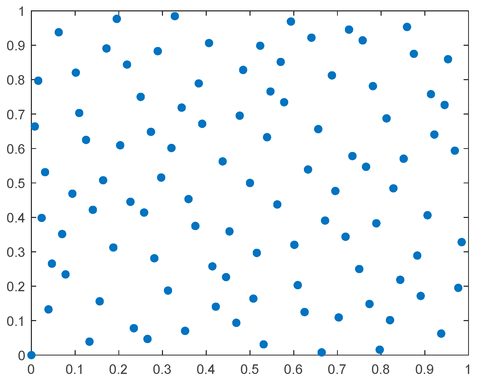
where $S_{i,j}$ is the Sobol sequence value belonging to [0, 1]. We set the search space dimension as D = 2 and population as N = 100, assuming that the lower and upper bounds are 0 and 1, respectively. The initial population distribution based on the Sobol sequence and random initialization is shown in Figure 1 and Figure 2. It was found that the initial population based on Sobol sequence is more evenly distributed and more diverse.

3.2. Weibull Distribution Step Factor

In the IOOA, random numbers subject to Weibull distribution are introduced into the position update process of phase 1 of the osprey optimization algorithm as a step factor. The probability density function of Weibull distribution is shown in Equation (11):

$$f\left(x;\lambda ,k\right)=\left\{\begin{array}{c}\frac{k}{\lambda }{\left(\frac{x}{\lambda }\right)}^{k-1}·e^{-{\left(\frac{x}{\lambda }\right)}^k},x\ge 0\\ 0,x<0\end{array}\right.$$

(11)

where $x$ is a random variable, $\lambda >0$ is the scale parameter, and $k>0$ is the shape parameter. It is introduced into the osprey position update expression (4) in phase 1 of the osprey optimization algorithm, and a new position update formula is obtained, as shown in Equation (12):

$$X_{i,j}^{P1}=X_{i,j}+{wblrnd}_{i,j}·\left({SF}_{i,j}-I_{i,j}·X_{i,j}\right),i=\mathrm{1,2},\cdots ,N;j=\mathrm{1,2},\cdots ,D$$

(12)

where ${wblrnd}_{i,j}$ is a random step factor subject to Weibull distribution, the scale parameter is 1, and the shape parameter is 0.5.

3.3. Firefly Disturbance

In this study, after the osprey optimization algorithm passed phase 2, a disturbance strategy based on the Firefly Algorithm (FA) was adopted for all osprey populations. When the firefly’s position is updated, the most important factors are changes in light intensity and attraction. In the FA, the light intensity $I$ varies monotonically and exponentially with distance r, and its relative fluorescence intensity I is:

$$I=I_0·e^{-\gamma r_{i,j}}$$

(13)

where $I_0$ is the maximum light intensity, and $\gamma$ is the absorption coefficient of light intensity, which this study takes as 0.01. The attraction between fireflies is proportional to the intensity of light seen by neighboring fireflies, and the attraction$\beta$ is defined as:

$$\beta ={\beta }_0·e^{-\gamma {r_{i,j}}^2}$$

(14)

where ${\beta }_0$ is the attraction at $r$ = 0, which is 1 in this study. Firefly $i$ is attracted to another more attractive (brighter) firefly $j$, and after being introduced to phase 2 of the OOA, it updates its position according to Equation (15). Then the boundary processing is carried out according to Equation (16):

$$X_i^{FA}=X_i^2+\beta \left(X_j^2-X_i^2\right)+\alpha (r-\frac{1}{2})$$

(15)

$$X_{i,j}^{FA}=\left\{\begin{array}{c}{X}_{i,j}^{FA},{lb}_j\le X_{i,j}^{FA}\le {ub}_j\\ {lb}_j,X_{i,j}^{FA}<{lb}_j\\ {ub}_j,X_{i,j}^{FA}>{ub}_j\end{array}\right.$$

(16)

where $X_i^2$, $X_j^2$ are the positions of firefly $i$ and $j$ after passing phase 2, respectively, and $X_i^{FA}$ is the positions after firefly disturbance. $\alpha$ belongs to [0, 1] and is taken as 0.2 in this study. $r$ is a random number that follows a uniform distribution [0, 1]. If the fitness value of the position updated by Equations (15) and (16) is better, the previous position is replaced. According to Equation (17), the updated position of osprey at this stage is obtained:

$$X_i^F=\left\{\begin{array}{c}{X}_{i,j}^{FA},F_i^{FA}<F_i^{P2}\\ X_i^2,F_i^{FA}\ge F_i^{P2}\end{array}\right.$$

(17)

where $F_i^{FA}$ is the fitness value of position $X_i^{FA}$; $X_i^F$ is the position of the $i$th osprey after the disturbed stage.

3.4. The IOOA Algorithm Flow

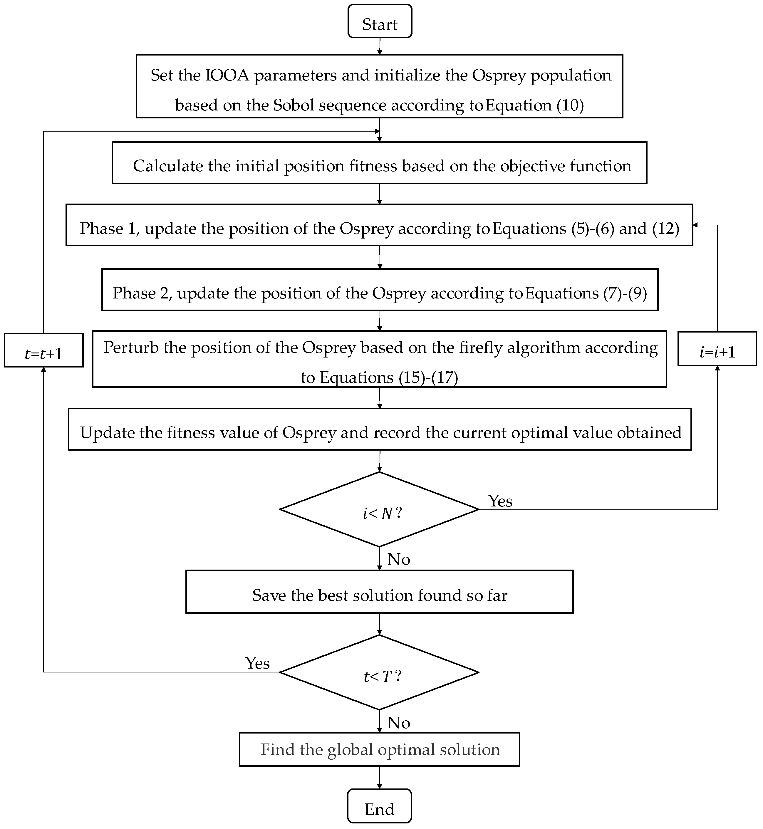
The improved osprey optimization algorithm (IOOA) is proposed in this paper. The specific process is as follows. First, an osprey population initialization strategy based on the Sobol sequence is adopted to make the first-generation population more evenly distributed in the search space and increase the diversity of the initial population due to the excellent uniformity and low diversity of the Sobol sequence. The step factor based on Weibull distribution is introduced in the first stage of the OOA, which improves the balance between the algorithm’s exploration and development, making the algorithm less prone to local optimization. Finally, the disturbance strategy based on the firefly optimization algorithm is introduced to mutate and disturb the position of the osprey population so that the OOA has a more vital ability to escape from local optimal. Through the above three strategies, the performance of the osprey optimization algorithm is comprehensively improved. The proposed IOOA algorithm flow and the proposed IOOA algorithm flow are shown in Figure 3.

4. Simulation Experiment of CEC Test Function

4.1. Experimental Scheme

In order to evaluate the performance of the proposed IOOA, 29 CEC2017 [41] test function suites were selected in this paper to conduct two experiments: a numerical experiment and an iterative curve analysis experiment. Since the CEC02 function has been officially stated to be unstable it was not selected for this experiment. CEC2017 test functions specifically include unimodal function UM (CEC01, CEC03), multi-modal function MM (CEC04–CEC10), mixed function H (CEC11–CEC20), and combined function C (CEC21–CEC30). For details, see Appendix A. All experiments used Intel(R) Core (TM) i7-7700HQ 2.80 GHz. The simulation experiment platform was Matlab R2022a and was carried out on a computer with 16 G of memory.

In this experiment, the proposed IOOA is compared with some widely used and advanced optimization algorithms: particle swarm optimization algorithm (PSO), whale optimization algorithm (WOA), butterfly optimization algorithm (BOA) and osprey optimization algorithm (OOA). The algorithms in the experiment are all standard parameters in the original text. For details, see Appendix B. In order to not lose generality and fairness, the population number of all the algorithms in this experiment is set to 30, and the maximum number of iterations T is 500.

4.2. Numerical Simulation Experiment and Analysis

In the numerical experiment part of the experiment, all of the algorithms were independently run 30 times when testing all CEC2017 test functions, the mean and standard deviation Std were recorded, and all of the algorithms were compared separately. The final experimental results are shown in

Table 1. Numerical comparison between IOOA and various algorithms on CEC2017 test functions.

CEC	PSO		WOA		BOA		OOA		IOOA
	Mean	Std	Mean	Std	Mean	Std	Mean	Std	Mean	Std
CEC01	4.45 × 109	2.19 × 109	5.36 × 109	2.08 × 109	5.47 × 1010	8.20 × 109	5.74 × 1010	8.96 × 109	4.52 × 104	9.93 × 103
CEC03	2.03 × 105	9.00 × 104	2.54 × 105	7.74 × 104	8.19 × 104	8.01 × 103	9.12 × 104	7.85 × 103	3.00 × 102	3.18 × 10−2
CEC04	1.60 × 103	1.21 × 103	1.33 × 103	3.57 × 102	2.08 × 104	4.03 × 103	1.63 × 104	2.91 × 103	4.91 × 102	3.45 × 101
CEC05	7.95 × 102	4.29 × 101	8.71 × 102	6.81 × 101	9.16 × 102	2.71 × 101	9.16 × 102	4.39 × 101	7.72 × 102	3.39 × 101
CEC06	6.56 × 102	1.44 × 101	6.79 × 102	1.13 × 101	6.90 × 102	6.25 × 101	6.87 × 102	6.43 × 101	6.62 × 102	3.46 × 101
CEC07	1.15 × 103	6.04 × 101	1.30 × 103	8.27 × 101	1.40 × 103	4.62 × 101	1.44 × 103	5.23 × 101	1.29 × 103	4.79 × 101
CEC08	1.07 × 103	4.46 × 101	1.07 × 103	6.45 × 101	1.14 × 103	2.01 × 101	1.13 × 103	2.22 × 101	9.66 × 102	2.53 × 101
CEC09	6.99 × 103	2.84 × 103	1.11 × 104	4.18 × 103	1.11 × 104	1.54 × 103	9.96 × 103	1.58 × 103	5.20 × 103	6.55 × 102
CEC10	7.71 × 103	7.11 × 102	7.56 × 103	7.21 × 102	9.25 × 103	4.02 × 102	8.60 × 103	4.34 × 102	5.72 × 103	7.85 × 102
CEC11	5.21 × 103	4.39 × 103	9.87 × 103	4.61 × 103	8.44 × 103	2.30 × 103	9.29 × 103	2.28 × 103	1.26 × 103	6.79 × 101
CEC12	8.31 × 108	9.45 × 108	5.88 × 108	2.84 × 108	1.41 × 1010	5.25 × 109	1.37 × 1010	3.90 × 109	2.91 × 107	1.56 × 108
CEC13	5.83 × 108	1.31 × 109	9.09 × 106	8.15 × 106	1.15 × 1010	6.67 × 109	8.96 × 109	4.96 × 109	1.37 × 105	7.07 × 104
CEC14	2.84 × 106	5.10 × 106	3.08 × 106	3.52 × 106	6.72 × 106	1.20 × 107	4.62 × 106	5.04 × 106	7.11 × 104	3.42 × 105
CEC15	1.33 × 106	1.16 × 106	3.79 × 106	5.92 × 106	4.97 × 108	3.62 × 108	5.37 × 108	3.99 × 108	2.20 × 104	1.47 × 104
CEC16	3.71 × 103	3.87 × 102	4.28 × 103	6.56 × 102	7.59 × 103	1.80 × 103	5.74 × 103	1.10 × 103	2.99 × 103	3.58 × 102
CEC17	2.67 × 103	3.36 × 102	2.83 × 103	2.69 × 102	1.18 × 104	1.18 × 104	4.66 × 103	2.90 × 103	2.62 × 103	2.28 × 102
CEC18	1.61 × 107	4.71 × 107	1.82 × 107	2.30 × 107	9.12 × 107	1.04 × 108	7.97 × 107	1.03 × 108	7.54 × 105	2.63 × 106
CEC19	2.67 × 107	4.04 × 107	1.96 × 107	2.45 × 107	8.22 × 108	5.79 × 108	6.93 × 108	6.25 × 108	1.59 × 104	1.09 × 104
CEC20	2.83 × 103	2.10 × 102	2.89 × 103	2.24 × 102	3.13 × 103	1.41 × 102	2.97 × 103	1.80 × 102	2.77 × 103	2.09 × 102
CEC21	2.59 × 103	3.57 × 101	2.65 × 103	5.27 × 101	2.71 × 103	6.79 × 101	2.71 × 103	4.60 × 101	2.59 × 103	3.88 × 101
CEC22	7.72 × 103	2.57 × 103	7.64 × 103	2.19 × 103	7.11 × 103	1.07 × 103	9.33 × 103	1.05 × 103	3.18 × 103	1.78 × 103
CEC23	3.31 × 103	2.34 × 102	3.15 × 103	8.67 × 101	3.52 × 103	1.63 × 102	3.73 × 103	1.46 × 102	3.24 × 103	1.07 × 102
CEC24	3.70 × 103	2.27 × 102	3.27 × 103	9.55 × 101	4.09 × 103	2.57 × 102	4.08 × 103	2.83 × 102	3.36 × 103	1.65 × 102
CEC25	3.27 × 103	1.46 × 102	3.22 × 103	7.02 × 101	5.71 × 103	6.12 × 102	5.06 × 103	5.13 × 102	2.89 × 103	1.77 × 101
CEC26	7.64 × 104	1.87 × 103	8.45 × 103	8.85 × 102	1.17 × 104	1.14 × 103	1.14 × 104	9.18 × 102	6.97 × 103	2.28 × 103
CEC27	3.76 × 103	4.01 × 102	3.47 × 103	1.26 × 102	4.39 × 103	3.74 × 102	4.83 × 103	4.58 × 102	3.50 × 103	2.56 × 102
CEC28	3.98 × 103	5.24 × 102	3.87 × 103	2.06 × 102	8.17 × 103	5.56 × 102	7.45 × 103	7.10 × 102	3.59 × 103	2.82 × 102
CEC29	4.82 × 103	5.05 × 102	5.35 × 103	5.34 × 102	1.48 × 104	1.04 × 104	9.01 × 103	4.77 × 103	4.53 × 103	3.52 × 102
CEC30	1.41 × 108	6.51 × 108	6.62 × 107	5.78 × 107	1.97 × 109	1.12 × 109	1.76 × 109	1.03 × 109	1.26 × 105	9.74 × 104

.

The performance of the proposed IOOA is analyzed in Table 1. CEC01 and CEC03 are unimodal functions, there is only a single extreme value: the main test algorithm development ability. For CEC01 and CEC03, the proposed IOOA’s convergence rate is faster than the other algorithms’, and more accurate solutions are obtained after 500 iterations. CEC04-CEC10 is a multimodal function, which mainly tests the global exploration capability of the function. The results obtained by the IOOA for CEC06 and CEC07 are slightly worse than those obtained by PSO, but on other multi-modal functions IOOA shows better global optimization ability and convergence to better values. For mixed function and combined function CEC11-CEC30, the comprehensive optimization performance of the algorithm can be evaluated. From the results, IOOA only achieved slightly worse results than WOA on functions CEC23, CEC24, and CEC27. IOOA has the smallest mean and standard deviation on other functions, and has significant advantages compared to other algorithms.

Overall, of the mean and standard deviations recorded by each algorithm after 30 independent runs, the proposed IOOA had the smallest mean (Mean) and the smallest standard deviation (Std) for most CEC2017 test functions. Thus, it also shows that the IOOA has higher optimization accuracy and robustness than other algorithms and verifies the feasibility and effectiveness of the improvement strategy used in this paper for the OOA.

4.3. Experimental Analysis of Iterative Curve

In the iteration curve simulation part of the experiment, all of the algorithms ran the CEC2017 test function 30 times, with the maximum number of iterations as the horizontal coordinate and the average value of the best value obtained by each algorithm running 30 times (the average value of the best fitness) as the vertical coordinate. The algorithm iteration curve simulation diagram is drawn. The performance of each algorithm is compared visually, and the iterative curve convergence diagram of some functions is shown in Figure 4.

The experimental results of five optimization algorithms are analyzed, combined with the iterative curve simulation experiment. In general, the proposed IOOA converges faster than the compared algorithms in most cases and converges to a more accurate value after 500 iterations. The proposed IOOA has a faster convergence rate in the early stage of iteration, as shown in Figure 4, precisely because the population initialization strategy based on the Sobol sequence is introduced. The introduction of the Weibull distribution step factor and firefly perturbation makes the IOOA show better global search ability than the compared optimization algorithms in the iterative process and converges to a better value under the same conditions.

4.4. Statistical Test

In order to compare the optimization performance of various algorithms more comprehensively, statistical tests are needed [42]. In this study, the Wilcoxon rank sum test was performed based on the experimental results of 30 runs of each algorithm on 29 CEC2017 test functions, and the p-values of significance level was set at 0.05. If the p-values obtained by the rank sum test is less than 0.05, it can be considered that the optimization performance of the IOOA is significantly different from that of the compared algorithm. For 29 benchmark functions, the IOOA’s p-values calculated in the Wilcoxon rank sum test with the compared algorithm are shown in

Table 2. p-values of Wilcoxon rank sum test for IOOA and other algorithms on CEC2017.

Function	IOOA VS
	PSO	WOA	BOA	OOA
CEC01	3.0199 × 10−11	3.0199 × 10−11	3.0199 × 10−11	3.0199 × 10−11
CEC03	3.0199 × 10−11	3.0199 × 10−11	3.0199 × 10−11	3.0199 × 10−11
CEC04	3.0199 × 10−11	3.0199 × 10−11	3.0199 × 10−11	3.0199 × 10−11
CEC05	1.1536 × 10−1	2.2273 × 10−9	3.3384 × 10−11	3.3384 × 10−11
CEC06	-	2.2273 × 10−9	3.0199 × 10−11	3.0199 × 10−11
CEC07	-	8.7663 × 10−1	2.2273 × 10−9	1.0937 × 10−10
CEC08	2.1544 × 10−10	2.1544 × 10−10	3.0199 × 10−11	3.0199 × 10−11
CEC09	1.0763 × 10−2	2.0338 × 10−9	3.0199 × 10−11	3.0199 × 10−11
CEC10	1.5465 × 10−9	4.1825 × 10−9	3.3384 × 10−11	7.3891 × 10−11
CEC11	3.0199 × 10−11	3.0199 × 10−11	3.0199 × 10−11	3.0199 × 10−11
CEC12	2.8716 × 10−10	2.8716 × 10−10	3.0199 × 10−11	3.0199 × 10−11
CEC13	3.0199 × 10−11	4.5043 × 10−11	3.0199 × 10−11	3.0199 × 10−11
CEC14	5.0723 × 10−10	1.7769 × 10−10	6.6955 × 10−11	8.9934 × 10−11
CEC15	3.0199 × 10−11	3.6897 × 10−11	3.0199 × 10−11	3.0199 × 10−11
CEC16	1.2023 × 10−8	1.6132 × 10−10	3.0199 × 10−11	3.0199 × 10−11
CEC17	5.4933 × 10−1	4.0330 × 10−3	4.9752 × 10−11	2.0152 × 10−8
CEC18	2.2273 × 10−9	3.8202 × 10−10	4.5043 × 10−11	7.3891 × 10−11
CEC19	3.0199 × 10−11	3.0199 × 10−11	3.0199 × 10−11	3.0199 × 10−11
CEC20	4.8252 × 10−1	4.7460 × 10−2	1.2023 × 10−8	4.7138 × 10−4
CEC21	2.9727 × 10−1	1.2493 × 10−5	8.4848 × 10−9	2.3715 × 10−10
CEC22	1.6947 × 10−9	1.6947 × 10−9	2.0152 × 10−8	3.3384 × 10−11
CEC23	3.1830 × 10−1	-	9.2603 × 10−9	4.5043 × 10−11
CEC24	1.5964 × 10−7	-	4.9752 × 10−11	4.9752 × 10−11
CEC25	3.0199 × 10−11	3.0199 × 10−11	3.0199 × 10−11	3.0199 × 10−11
CEC26	5.2014 × 10−1	9.0688 × 10−3	8.1527 × 10−11	3.0199 × 10−11
CEC27	1.9527 × 10−3	-	3.8202 × 10−10	4.0772 × 10−11
CEC28	1.3703 × 10−3	1.2362 × 10−3	3.0199 × 10−11	3.0199 × 10−11
CEC29	3.9167 × 10−2	1.0666 × 10−7	3.0199 × 10−11	3.0199 × 10−11
CEC30	3.0199 × 10−11	3.0199 × 10−11	3.0199 × 10−11	3.0199 × 10−11
+/=/−	21/6/2	26/1/3	29/0/0	29/0/0

.

In Table 2, ‘+’, ‘=‘, and ‘−’, respectively, indicate that the performance of the proposed IOOA is “better”, “same”, and “worse” compared with the compared algorithms. According to the results obtained in the last row of Table 2, the IOOA proposed for most CEC2017 test functions has a large difference in statistical tests compared with the compared algorithms, and most of the p-values are far less than 0.05, which further verifies the effectiveness and superiority of the proposed IOOA.

4.5. Effectiveness Analysis of Single Improvement Strategy

In this section, the effectiveness analysis experiment of the improvement strategy is carried out in order to further verify whether the three improvement strategies adopted to improve the osprey optimization algorithm are effective. We separately introduced each strategy into the osprey optimization algorithm, namely SOOA using only Sobol sequence initialization, WOOA using only Weibull step factor, and FOOA using only firefly disturbance. The experiments are compared with standard OOA and our proposed IOOA, respectively. We selected some representative test functions from CEC2017, namely single-peak F1, multi-peak F4, mixed functions F12 and F17, and combined functions F22 and F27, to carry out comparative experiments of algorithms. The experimental scheme is the same as the previous experiment.

Finally, the experimental results of the iterative curve obtained are shown in Figure 5. From the figure, we can see that each of the strategies adopted has a positive effect on OOA performance. Additionally, the proposed IOOA’s mixed three strategies have faster convergence speeds and convergence accuracy, and better optimization performance. To sum up, it can be reflected that our improvement strategy for the OOA is very effective and comprehensively improves the optimization performance of the OOA.

5. Reactive Power Optimization Application of Distribution Network Based on IOOA

5.1. Reactive Power Optimization Model of Distribution Network

5.1.1. Objective Function

In this study, the objective function is that the voltage of each node does not exceed the limit and the active power network loss $P_{loss}$ of the system is minimum. Among them, the voltage exceedance is added to the objective function in the form of penalty function, and the final objective function is obtained as shown in Equation (18):

$$\min F=P_{loss}+\alpha {\sum }_{i=1}^{N_n}\left(\frac{∆U_i}{U_{i\_max}-U_{i\_min}}\right)$$

(18)

$$P_{loss}={\sum }_{i=1}^{N_B}{G}_b\left(U_i^2+U_i^2-2U_i{U}_j\cos {\theta }_{ij}\right)$$

(19)

$$∆U_i=\left\{\begin{array}{c}{U}_{i\_min}-U_i,U_i<U_{i\_min}\\ 0,U_{i\_min}\le U_i\le U_{i\_max}\\ U_i-U_{i\_max},U_{i\_max}{<U}_i\end{array}\right.$$

(20)

where $N_n$ is the number of nodes in the distribution network system, $U_i$ is the voltage amplitude of node $i$, $∆U_i$ is the voltage offset of node $i$, $U_{i\_max}$ is the upper limit of voltage, $U_{i\_min}$ is the lower limit of voltage, α is the penalty factor, $N_B$ is the number of branches of the system, and $G_b$ is the conductance of branch b.

5.1.2. Constraints

(1) Equality constraint

The power flow constraint is an equality constraint. Its expression is:

$$\left\{\begin{array}{c}{P}_i=U_i{\sum }_{j=1}^{N_n}{U}_j\left(G_{ij}\cos {\theta }_{ij}+B_{ij}\sin {\theta }_{ij}\right)\\ Q_i=U_i{\sum }_{j=1}^{N_n}{U}_j\left(G_{ij}\sin {\theta }_{ij}-B_{ij}\cos {\theta }_{ij}\right)\end{array}\right.$$

(21)

where $P_i$ is the active power injected by node $i$, $Q_i$ is the reactive power injected by node $i$, $G$ is the conductance of the branch, and $B$ is the susceptance of the branch.

(2) Inequality constraints

Inequality constraints include control variable constraints and state variable constraints. The constraint expression for the control variable is:

$$\left\{\begin{array}{c}{Q}_{DGi}^{min}\le Q_{DGi}\le Q_{DGi}^{max}\\ Q_{Ci}^{min}\le Q_{Ci}\le Q_{Ci}^{max}\end{array}\right.$$

(22)

where $Q_{DGi}$ is the capacity of the $i$th distributed power supply connected to the system, and $Q_{Ci}$ is the capacity of the parallel reactive power compensation device. $min$ and $max$ represent the lower and upper limits of each control variable, respectively. The state variable is the voltage amplitude of each node in the system, and its constraint is expressed as:

$$U_{i\_min}\le U_i\le U_{i\_max}.$$

(23)

5.2. Analysis and Verification of Calculation Examples

5.2.1. Modified IEEE33 Node System

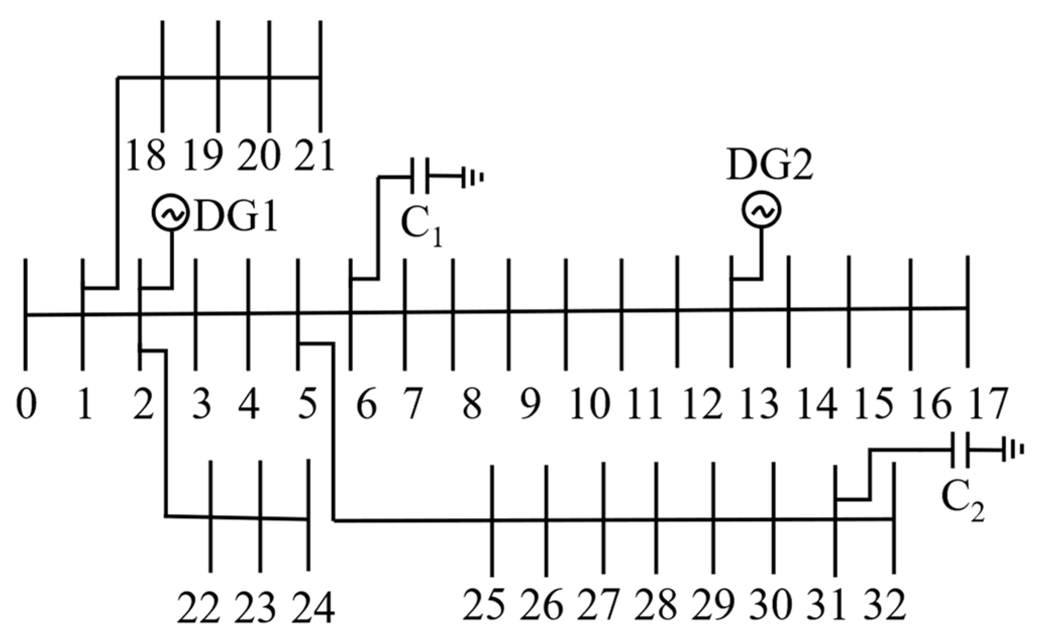
In this study, the IEEE33-node power distribution system is used as the test system to verify the feasibility and effectiveness of the proposed IOOA. The specific parameters of the test system can be found in reference [43]. In the test system, node 0 is taken as the balance node, the reference value of three-phase power is 10 MVA, the voltage range of each node is 0.9 p.u.–1.1 p.u., and the reference value of line voltage is 12.66 KV. Distributed power supply DG1 and DG2 are connected to nodes 2 and 13, respectively. The upper limit of reactive power output of each DG is 500 KVar, the lower limit is −100 KVar, and the active power output is 1 MW. Parallel compensation capacitors $C_1$ and $C_2$ are at nodes 6 and 31, each group of capacitors has a reactive power output of 150 KVar, the upper limit of each group of capacitors is seven groups, and the lower limit is zero groups. To sum up, the modified IEEE33 node test system is obtained, as shown in Figure 6.

5.2.2. Reactive Power Optimization and Result Analysis

The simulation experiment of programming and reactive power optimization is carried out on Matlab R2022a, and the power flow of the test system is calculated using Matpower 7.0. The proposed IOOA is compared with PSO, WOA, BOA, and OOA, which are the most widely used particle swarm optimization algorithms. In the experiment, in order to reflect the fairness of the experiment, the population size of all algorithms was set to 10, and the maximum number of iterations was set to 100. The main parameters of each algorithm are set according to CEC test function simulation experiment.

All algorithms were independently run 30 times, and the average value and standard deviation of the minimum active network loss obtained by each algorithm were shown in

Table 3. IEEE33 active network loss obtained by running IOOA and other algorithms 30 times.

${\mathit{P}}_{\mathit{l}\mathit{o}\mathit{s}\mathit{s}}$/KW	PSO	WOA	BOA	OOA	IOOA
Mean	65.0022	65.1889	65.0782	65.0585	64.9461
std	7.9252 × 10−2	1.1696 × 10−1	1.1222 × 10−1	6.1289 × 10−2	2.3611 × 10−3

. It can be seen from the results that compared with the PSO, WOA, BOA, and OOA, the average net loss obtained by the IOOA is smaller, and the standard deviation is also smaller. That is, compared with other algorithms, the optimization performance is better, and it has higher robustness. After using the IOOA for reactive power optimization, the active power network loss of the example system is reduced from the initial state of 126.6119 KW to 64.9461 KW, and the loss reduction rate reaches 48.7%.

The average fitness iteration curve of each algorithm running 30 times is shown in Figure 7. Compared with the PSO, although the PSO has a faster iteration speed at the beginning, the IOOA has a faster iteration speed later, and finally converges to a better value than PSO. Compared to the WOA, BOA, and OOA, the IOOA is faster and has higher optimization accuracy. In summary, the active power loss obtained by the IOOA is smaller than that of the compared algorithms under the same conditions, which verifies the feasibility of applying the IOOA to reactive power optimization and is more stable than other compared algorithms.

The configurations of each control variable obtained by each algorithm are shown in

Table 4. Control variable values after reactive power optimization of all algorithms on IEEE33.

Node	Control Variable	Initial Value	PSO	WOA	BOA	OOA	IOOA
2	DG1	0	467.1237	319.8047	362.2881	496.8163	500
13	DG2	0	315.9137	264.6881	305.9574	306.3683	300.6098
6	C1	0	150 × 5	150 × 5	150 × 5	150 × 5	150 × 4
31	C2	0	150 × 5	150 × 5	150 × 5	150 × 5	150 × 5

after reactive power optimization. In the proposed IOOA, DG1 output is 500 KVar, DG2 output is 300.6098 KVar, $C_1$ input five groups, and $C_2$ input four groups, which is less than one group of compensation capacitors required by other algorithms and more economical.

The voltage distribution of each node of the IEEE33-node system before and after the optimization of each algorithm is shown in Figure 8. It can be seen that the node voltage after the optimization of each algorithm has been increased to 0.95 p.u. Above this, the voltage distribution is more stable. Compared with the other algorithm, the voltage of each node after IOOA optimization is 0.96 p.u. Above this, the voltage stability is better, has higher power quality, and is more in line with the safe operation requirements of the distribution system. Through the example of reactive power optimization, the feasibility and effectiveness of the IOOA applied to reactive power optimization are further verified.

5.3. Example Analysis of IEEE69 Node System

5.3.1. Modified IEEE69 Node System

In this section, the IEEE69 node power distribution system is modified. Distributed power supplies DG1, DG2, and DG3 are connected to nodes 2, 5, and 56, respectively. The upper limit of reactive power output of each DG is 500 KVar, the lower limit is −100 KVar, and the active power output is 1 MW. Parallel compensation capacitors at nodes 16, 58, and 63, and each group of capacitors has a reactive power output of 150 KVar, each group of capacitors has an upper limit of seven groups and a lower limit of zero groups. Figure 9 shows the modified IEEE69 node power distribution system. The reference value of three-phase power is 10 MVA. The voltage of each node ranges from 0.9 p.u. to 1.1 p.u. The reference value of the line voltage is 12.66 KV and its unit value is 1.0 p.u.

5.3.2. Result Analysis

The experimental setup is the same as that of IEEE33-node system. The average value and standard deviation of the minimum active power network loss obtained by each algorithm on the IEEE69 node system after reactive power optimization are shown in

Table 5. IEEE69 active network loss obtained by running IOOA and other algorithms 30 times.

${\mathit{P}}_{\mathit{l}\mathit{o}\mathit{s}\mathit{s}}$/KW	PSO	WOA	BOA	OOA	IOOA
Mean	101.9096	102.3257	104.7994	102.9333	101.5090
Std	4.7382 × 10−3	6.7928 × 10−2	7.3306 × 10−1	8.7070 × 10−2	3.9557 × 10−3

. The IEEE69 node system is more complex than the IEEE33 node system, and the addition of distributed power supply and capacitance in this example makes the reactive power optimization more difficult; however, our proposed IOOA also obtains a smaller active power network loss value, which is more accurate than the other advanced algorithms we compared. IEEE69’s active network loss after IOOA optimization is reduced from 175.4171 KW to 101.5090 KW, a loss reduction of 42.1%.

In the case of IEEE69, the average fitness iteration curve of each algorithm running 30 times is shown in Figure 10. It can be seen that the BOA falls into local optimization quickly, while the PSO, WOA, and OOA are faster than the IOOA at the beginning of iteration, but they advance quickly. The proposed IOOA has a stronger ability to avoid local optimality and converges to a more accurate value at a faster speed.

The configurations of each control variable obtained by each algorithm after reactive power optimization are shown in

Table 6. Control variable values after reactive power optimization of all algorithms on IEEE69.

Node	Control Variable	Initial Value	PSO	WOA	BOA	OOA	IOOA
2	DG1	0	179.3693	−86.1497	306.1118	288.4188	168.2511
5	DG2	0	500	38.18137	464.3374	311.4348	346.2607
56	DG3	0	221.1304	202.3876	165.7195	72.2129	218.4523
16	C1	0	150 × 2	150 × 2	150 × 3	150 × 2	150 × 2
58	C2	0	150 × 2	150 × 3	150 × 3	150 × 4	150 × 2
63	C3	0	150 × 7	150 × 6	750 × 5	150 × 5	150 × 7

.

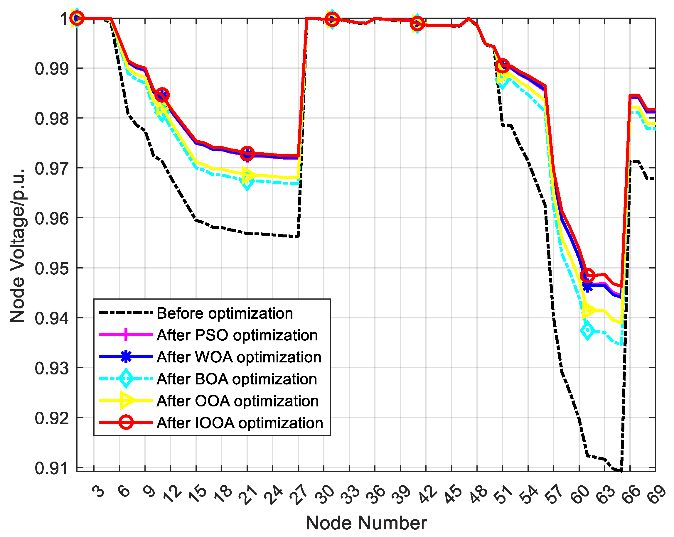
The voltage distribution of all nodes in the IEEE69 node system before and after the optimization of each algorithm is shown in Figure 11. The voltage fluctuates greatly before the reactive power optimization, and the node voltage after the optimization of each algorithm is more stable. Moreover, the node voltage obtained after the proposed IOOA optimization is the most stable, which makes the IEEE69 node distribution network run more safely and stably.

6. Discussion and Conclusions

Three strategies are proposed to improve the osprey optimization algorithm and good results were achieved based on the characteristics of the osprey optimization algorithm to solve the reactive power optimization problem of distribution network. First, Sobol sequence initialization strategy is used instead of random initialization. Secondly, The step factor based on Weibull distribution is introduced in updating the position of osprey. Finally, after phase 2, the osprey position was disturbed based on the fire fly algorithm. Based on the mixed improvement of the above three strategies, we propose an IOOA algorithm with better performance. The effectiveness of the proposed IOOA algorithm is verified by experiments on 29 CEC2017 test functions. Compared with other advanced algorithms, the IOOA has a faster optimization speed, higher robustness, and a higher ability to jump out of the local optimal. In the application of IEEE33 and IEEE69 node distribution network reactive power optimization, smaller active power network loss and voltage fluctuation are obtained by using IOOA optimization, and the optimized active power network loss is reduced by 48.7% and 42.1%, respectively, which shows that it also has great advantages in solving practical multi-dimensional and multi-constraint problems. In addition, it advantages over other algorithms. In future work, we will further apply the IOOA to more complex IEEE node systems and other practical optimization problems to fully verify its good performance and explore its application potential in different optimization problems.

References

1. Xiang, Y.; Zhou, L.; Huang, Y.; Zhang, X.; Liu, Y.; Liu, J. Reactive coordinated optimal operation of distributed wind generation. Energy 2021, 218, 119417. [Google Scholar] [CrossRef]
2. Hu, D.; Ye, Z.; Gao, Y.; Ye, Z.; Peng, Y.; Yu, N. Multi-Agent Deep Reinforcement Learning for Voltage Control with Coordinated Active and Reactive Power Optimization. IEEE Trans. Smart Grid 2022, 13, 4873–4886. [Google Scholar] [CrossRef]
3. Xiao, H.; Pei, W.; Dong, Z.; Pu, T.; Chen, N.; Kong, L. Reactive power optimization of distribution network with distributed power based on meta-model global optimization. Proc. CSEE 2018, 38, 5751–5762. [Google Scholar]
4. Niazi, Y.; Golshan, M.E.H.; Alhelou, H.H. Combined Firm and Renewable Distributed Generation and Reactive Power Planning. IEEE Access 2021, 9, 133735–133745. [Google Scholar] [CrossRef]
5. Delson, J.K.; Shahidehpour, S.M. Linear programming applications to power system economics. Planning and Operations. IEEE Trans. Power Syst. 1992, 7, 1155–1163. [Google Scholar] [CrossRef]
6. Lai, L.L.; Ma, J.T. Application of evolutionary programming to reactive power planning-comparison with nonlinear programming approach. IEEE Trans. Power Syst. 1997, 12, 198–206. [Google Scholar] [CrossRef]
7. Pang, B.; Long, W.; Hu, L. Development & Application of Reactive Power Optimization Software for Regional Power Network. In Proceedings of the 2009 International Conference on Intelligent Human-Machine Systems and Cybernetics, Hangzhou, China, 26–27 August 2009; pp. 376–379. [Google Scholar] [CrossRef]
8. Zhang, C.; Chen, H.; Shi, K.; Liang, Z.; Mo, W.; Hua, D. A Multi-time Reactive Power Optimization Under Interval Uncertainty of Renewable Power Generation by an Interval Sequential Quadratic Programming Method. IEEE Trans. Sustain. Energy 2019, 10, 1086–1097. [Google Scholar] [CrossRef]
9. Nazir, R.; Kanada, K.; Syafii; Coveria, P. Optimization Active and Reactive Power Flow for PV Connected to Grid System Using Newton Raphson Method. Energy Procedia 2015, 68, 77–86. [Google Scholar] [CrossRef]
10. Zhao, J.; Ju, L.; Dai, Z.; Chen, G. Voltage stability constrained dynamic optimal reactive power flow based on branch-bound and primal–dual interior point method. Int. J. Electr. Power Energy Syst. 2015, 73, 601–607. [Google Scholar] [CrossRef]
11. Yang, M.; Li, J.; Du, R.; Li, J.; Sun, J.; Yuan, X.; Xu, J.; Huang, S. Reactive Power Optimization Model for Distribution Networks Based on the Second-Order Cone and Interval Optimization. Energies 2022, 15, 2235. [Google Scholar] [CrossRef]
12. Shaheen, M.A.M.; Hasanien, H.M.; Alkuhayli, A. A novel hybrid GWO-PSO optimization technique for optimal reactive power dispatch problem solution. Ain Shams Eng. J. 2021, 12, 621–630. [Google Scholar] [CrossRef]
13. Elsheikh, A.H.; Abd Elaziz, M.; Vendan, A. Modeling ultrasonic welding of polymers using an optimized artificial intelligence model using a gradient-based optimizer. Weld World 2022, 66, 27–44. [Google Scholar] [CrossRef]
14. Abd Elaziz, M.; Elsheikh, A.H.; Oliva, D.; Abualigah, L.; Lu, S.; Ewees, A.A. Advanced Metaheuristic Techniques for Mechanical Design Problems: Review. Arch. Computat. Methods Eng. 2022, 29, 695–716. [Google Scholar] [CrossRef]
15. Fontes, D.B.M.M.; Homayouni, S.M.; Gonçalves, J.F. A hybrid particle swarm optimization and simulated annealing algorithm for the job shop scheduling problem with transport resources. Eur. J. Oper. Res. 2023, 306, 1140–1157. [Google Scholar] [CrossRef]
16. Elsheikh, A.H.; Muthuramalingam, T.; Abd Elaziz, M.; Ibrahim, A.M.M.; Showaib, E.A. Minimization of fume emissions in laser cutting of polyvinyl chloride sheets using genetic algorithm. Int. J. Environ. Sci. Technol. 2022, 19, 6331–6344. [Google Scholar] [CrossRef]
17. Morales, J.Y.R.; López, G.L.; Martínez, V.M.A.; Sorcia Vázquez, F.d.J.; Mendoza, J.A.B.; García, M.M. Parametric study and control of a pressure swing adsorption process to separate the water-ethanol mixture under disturbances. Sep. Purif. Technol. 2020, 236, 116214. [Google Scholar] [CrossRef]
18. Sorcia-Vázquez, F.D.J.; Garcia-Beltran, C.D.; Valencia-Palomo, G.; Brizuela-Mendoza, J.A.; Rumbo-Morales, J.Y. Decentralized robust tube-based model predictive control: Application to a four-tank-system. Rev. Mex. Ing. Química 2020, 19, 1135–1151. [Google Scholar] [CrossRef]
19. Elsheikh, A.H. Applications of machine learning in friction stir welding: Prediction of joint properties, real-time control and tool failure diagnosis. Eng. Appl. Artif. Intell. 2023, 121, 105961. [Google Scholar] [CrossRef]
20. Elsheikh, A.H.; Shehabeldeen, T.A.; Zhou, J.; Showaib, E.A.; Elaziz, M.E.A. Prediction of laser cutting parameters for polymethylmethacrylate sheets using random vector functional link network integrated with equilibrium optimizer. J. Intell. Manuf. 2021, 32, 1377–1388. [Google Scholar] [CrossRef]
21. Najjar, I.M.R.; Sadoun, A.M.; Elaziz, M.A.; Abdallah, A.W.; Fathy, A.; Elsheikh, A.H. Predicting kerf quality characteristics in laser cutting of basalt fibers reinforced polymer composites using neural network and chimp optimization. Alex. Eng. J. 2022, 61, 11005–11018. [Google Scholar] [CrossRef]
22. Moustafa, E.B.; Elsheikh, A. Predicting Characteristics of Dissimilar Laser Welded Polymeric Joints Using a Multi-Layer Perceptrons Model Coupled with Archimedes Optimizer. Polymers 2023, 15, 233. [Google Scholar] [CrossRef] [PubMed]
23. Rentería-Vargas, E.M.; Aguilar, C.J.Z.; Morales, J.Y.R.; De-La-Torre, M.; Cervantes, J.A.; Huerta, J.R.L.; Torres, G.O.; Vázquez, F.D.J.S.; Sánchez, R.O. Identification by Recurrent Neural Networks applied to a Pressure Swing Adsorption Process for Ethanol Purification. In Proceedings of the 2022 Signal Processing: Algorithms, Architectures, Arrangements, and Applications (SPA), Poznan, Poland, 21–22 September 2022; pp. 128–134. [Google Scholar] [CrossRef]
24. Liu, Y.; Ćetenović, D.; Li, H.; Gryazina, E.; Terzija, V. An optimized multi-objective reactive power dispatch strategy based on improved genetic algorithm for wind power integrated systems. Int. J. Electr. Power Energy Syst. 2022, 136, 107764. [Google Scholar] [CrossRef]
25. Antunes, C.H.; Lima, P.; Oliveira, E.; Pires, D.F. A multi-objective simulated annealing approach to reactive power compensation. Eng. Optim. 2011, 43, 1063–1077. [Google Scholar] [CrossRef]
26. Naderi, E.; Narimani, H.; Fathi, M.; Narimani, M.R. A novel fuzzy adaptive configuration of particle swarm optimization to solve large-scale optimal reactive power dispatch. Appl. Soft Comput. 2017, 53, 441–456. [Google Scholar] [CrossRef]
27. Lin, J.; Wang, X. Reactive Power Optimization Based on Adaptive Immune Algorithm. Int. J. Emerg. Electr. Power Syst. 2009, 10. [Google Scholar] [CrossRef]
28. Silas Stephen, D.; Somasundaram, P. Solution for Multi-Objective Reactive Power Optimization Using Fuzzy Guided Tabu Search. Arab J. Sci. Eng. 2012, 37, 2231–2241. [Google Scholar] [CrossRef]
29. Lian, L. Reactive power optimization based on adaptive multi-objective optimization artificial immune algorithm. Ain Shams Eng. J. 2022, 13, 101677. [Google Scholar] [CrossRef]
30. Zhang, W.; Liu, Y. Reactive power optimization based on PSO in a practical power system. In Proceedings of the IEEE Power Engineering Society General Meeting, Denver, CO, USA, 6–10 June 2004; Volume 1, pp. 239–243. [Google Scholar] [CrossRef]
31. Medani, K.B.O.; Sayah, S.; Bekrar, A. Whale optimization algorithm based optimal reactive power dispatch: A case study of the Algerian power system. Electr. Power Syst. Res. 2018, 163, 696–705. [Google Scholar] [CrossRef]
32. Singh, H.; Sawle, Y.; Dixit, S.; Malik, H.; Márquez, F.P.G. Optimization of reactive power using dragonfly algorithm in DG integrated distribution system. Electr. Power Syst. Res. 2023, 220, 109351. [Google Scholar] [CrossRef]
33. Wolpert, D.H.; Macready, W.G. No free lunch theorems for optimization. IEEE Trans. Evol. Comput. 1997, 1, 67–82. [Google Scholar] [CrossRef]
34. Dehghani, M.; Trojovský, P. Osprey optimization algorithm: A new bio inspired metaheuristic algorithm for solving engineering optimization problems. Front. Mech. Eng. 2023, 8, 1126450. [Google Scholar] [CrossRef]
35. Li, Y.; Han, M.; Guo, Q. Modified Whale Optimization Algorithm Based on Tent Chaotic Mapping and Its Application in Structural Optimization. KSCE J. Civ. Eng. 2020, 24, 3703–3713. [Google Scholar] [CrossRef]
36. Tubishat, M.; Idris, N.; Shuib, L.; Abushariah, M.A.M.; Mirjalili, S. Improved Salp Swarm Algorithm based on opposition based learning and novel local search algorithm for feature selection. Expert Syst. Appl. 2020, 145, 113122. [Google Scholar] [CrossRef]
37. Agushaka, O.J.; Ezugwu, A.E.-S. Influence of Initializing Krill Herd Algorithm With Low-Discrepancy Sequences. IEEE Access 2020, 8, 210886–210909. [Google Scholar] [CrossRef]
38. Hu, H.; Guo, J.; Wu, Y.; Nai, W.; Yang, Z.; Li, D. t-SNE Dimensionality Reduction Method Based on Sobol Sequence Initialized Archerfish Hunting Optimizer Algorithm. In Proceedings of the 2022 7th International Conference on Computational Intelligence and Applications (ICCIA), Nanjing, China, 24–26 June 2022; pp. 43–47. [Google Scholar] [CrossRef]
39. Yiwen, W.; Weili, W.; Yuge, Y.; Hui, Z. Multiple Strategy Fusion Algorithm Improved Marine Predators and Its Engineering Application [J/OL]. Computer Integrated Manufacturing System. pp. 1–21. Available online: https://kns-cnki-net.webvpn.jlju.edu.cn/kcms/detail/11.5946.TP.20230515.1111.008.html (accessed on 30 August 2023).
40. Yang, X.S. Firefly Algorithm, Stochastic Test Functions and Design Optimisation. Int. J. Bio-Inspired Comput. 2010, 2, 78–84. [Google Scholar] [CrossRef]
41. Awad, N.H.; Ali, M.; Liang, J.; Qu, B.; Suganthan, P. Problem Definitions and Evaluation Criteria for the CEC 2017 Special Session and Competition on Single Objective Bound Constrained Real-Parameter Numerical Optimization; Technical Report; Nanyang Technological University: Singapore, 2016. [Google Scholar]
42. Li, M.; Xu, G.; Lai, Q.; Chen, J. A chaotic strategy-based quadratic Opposition-Based Learning adaptive variable-speed whale optimization algorithm. Math. Comput. Simul. 2022, 193, 71–99. [Google Scholar] [CrossRef]
43. Wang, S.; Wang, C. Analysis of Modern Power Distribution System, 2nd ed.; Higher Education Press: Beijing, China, 2014. [Google Scholar]
Figure 1. Randomly initialized population distribution.
Energies 16 07101 g001
Figure 2. Population distribution of Sobol sequence initialization.
Energies 16 07101 g002
Figure 3. IOOA flow chart.
Energies 16 07101 g003
Figure 4. Comparison of IOOA and other algorithms on CEC2017 iterative curves.
Energies 16 07101 g004
Figure 5. Iteration curve of single strategy effectiveness analysis experiment.
Energies 16 07101 g005
Figure 6. Modified IEEE33 node system.
Energies 16 07101 g006
Figure 7. Comparison of fitness iteration curves of each algorithm on IEEE33 system.
Energies 16 07101 g007
Figure 8. Voltage distribution of each node after IOOA optimization on IEEE33 system.
Energies 16 07101 g008
Figure 9. Modified IEEE69 node system.
Energies 16 07101 g009
Figure 10. Comparison of fitness iteration curves of various algorithms on IEEE69.
Energies 16 07101 g010
Figure 11. Voltage distribution of nodes after optimization of algorithms on IEEE69.
Energies 16 07101 g011