A Methodological Approach of Predicting the Performance of Thermoelectric Generators with Temperature-Dependent Properties and Convection Heat Losses

Abstract

Thermoelectric generators are devices that transform thermal energy into electric energy. These devices play an influential role in our constantly developing civilization due to their energy conversion capabilities and advantages over other conventional methods. The material properties and thermoelectric phenomena are paramount to the design process of such devices. The design process must have a complex tool to model all the thermoelectric phenomena, such as, for example, the commercial numerical code of Ansys Mechanical. However, these numerical tools can be methodologically and computationally demanding. Thus, this study aims to develop a methodology through which to characterize thermoelectric generators by using a simplified one-dimensional numerical model that considers temperature-dependent N- and P-type material properties and convective heat losses. The proposed model’s results are compared and validated to a single thermoelectric leg and a complete thermoelectric commercial module, both modeled in Ansys Thermal-Electric. These results consider the different values for electric and thermal loads as current densities, electric resistivities, and heat transfer coefficients. The main result of this study is the correct prediction of the output voltage and output power given by the one-dimensional proposed model, which was validated against a comprehensive model and the commercial thermoelectric module’s information. Therefore, the proposed methodology of this study provides a deeper understanding of the thermoelectric energy conversion process, and it can guide the design and optimization of thermoelectric generators for practical applications.

1. Introduction

Thermoelectric (TE) materials are a type of functional energy material that can convert heat into electric power directly [1]. This approach has many advantages over traditional energy conversion methods, such as being noiseless, environmentally friendly, and requiring no maintenance [2]. In the automotive industry, it can convert waste heat from exhausts into electricity [3,4], and, in space exploration, it can convert the heat generated by electronic equipment into electricity by using radioisotope TEGs [5] (which also have uses in the field of biomedical devices for body heat measurements [6] and harvesting [7]). As a result, thermoelectric generators (TEGs) have been widely used for waste heat recovery and power generation, making them a versatile and promising technology for a wide range of applications. However, their low energy conversion efficiency has made it difficult for TEGs to be widely adopted [8]. The thermoelectric figure of merit (ZT) is a performance indicator for predicting the performance of TE materials. But, traditional methods of calculating ZT assume constant properties and disregard the temperature-dependent Thomson effect [9]. This can lead to significant errors in predictions when large temperature differences are present, as the properties of TE materials are highly dependent on temperature [10]. To obtain accurate results, it is essential to consider the temperature dependence of material properties when calculating TE power performance.

Several studies have addressed this issue by incorporating the Thomson effect into the analysis of TE performance. Guao et al. and Sun et al. found that the Thomson effect cannot be ignored in the analysis of thermoelectric generators [11,12]. Yamashita analyzed TE efficiency by accounting for both the linear and non-linear temperature dependence of material properties [13]. Additionally, in order to ensure the reliability of in-service TEGs, it is important to investigate and address thermal stress [14], thermal buckling [15], crack issues [16], and mismatches in thermal conditions [17]—all of which can be accurately analyzed by incorporating a temperature-dependent model. To improve the performance of thermoelectric materials, it is necessary to simultaneously increase the Seebeck coefficient, lower the electrical resistivity, and decrease the heat conductivity. Because these three properties are closely related, it can be challenging to change one without affecting the others. For example, lowering the electrical resistivity requires a high concentration of charge carriers, which may also increase heat conductivity. In contrast, increasing the Seebeck coefficient requires a modest charge carrier concentration. Over the past decade, scientists have made significant progress toward improving ZT by discovering new thermoelectric materials and new material structures with high performance, such as skutterudites with high scattering rates of phonons [18], silicon nanowires, thermoelectric thin films, and nanostructured bismuth selenide bulk alloys [19].

In practical engineering, convection heat losses at the legs of thermoelectric generators are unavoidable to some extent, and they can significantly impact energy conversion efficiency. Due to the complexity of the governing equations that consider temperature-dependent material properties, approximation methods have been employed to simplify the analysis. Wee [20] used a perturbation method to establish a linear temperature profile, while Ju et al. [21] improved upon this method to achieve a more accurate temperature expression. An analytic temperature solution that considers convection heat losses was developed by Wang [22], in which side surface heat convection for a single thermoelectric leg was considered. However, there is currently no methodological approach through which to model complete thermoelectric modules that consider the complex model of a single leg, as well as the other factors that affect the module’s performance. These factors include the variable material properties, the temperature dependence of these properties, the convection heat losses at the legs, the Thomson effect, and the Joule heat in the coupling connections.

Wielgosz et al. [23] discussed the importance of quantifying discretization uncertainty and scrutinizing the thermoelectric phenomena in the numerical models of thermoelectric generators to improve the predictions of their energy performance. Two models were developed and evaluated, a numeric model in Ansys CFX and an iterative analytic model, to address the issues identified. The results are compared with Ansys Thermal–Electric (TE) and Ansys Fluent. The article concluded that the inclusion of Thomson heat is imperative when modeling thermoelectric devices, and that the analytic model’s thermal and electrical performance predictions are sufficient for the thermal–electric characterization of unicouples with interconnectors that operate under certain conditions. Sreekala et al. [24] studied the functioning of coil guns, which use the electrical energy harvested from a bio-thermal energy harvester to fire multifunctional bullets, thus allowing them to be reused in an emergency without exploding. They used the Ansys model to study thermoelectric energy harvesting, which can be used to power specialized applications like medical devices by using the heat produced by the human body. Bhuiyan et al. [25] described the use of simulation in predicting the performance of TEG materials and the design of a TEG unit using Ansys; they also used mathematical modeling in MATLAB/Simulink to analyze the parameters of voltage, current, and power regarding the changes in a temperature gradient.

The first step in developing a methodological approach to model complete thermoelectric modules is establishing a mathematical model that describes the thermoelectric energy conversion process. This model should consider the temperature-dependent material properties of the thermoelectric and convection heat losses at the legs. Additionally, the Thomson effect should be included as it can significantly impact the module’s performance. The model should be established so that it can be solved by numerical methods to obtain a solution for the module’s temperature and energy conversion efficiency. This solution can then be used to optimize the module’s design for a specific application. This approach should be validated through experimental measurements for the specific thermoelectric materials and modules or reported data. The validation process allows for a confirmation of the accuracy and reliability of the proposed model and its predictions; it is an essential step in any model development. This paper aims to fill this gap by developing a solution that considers temperature-dependent material properties and convection heat losses. The proposed model for the analysis of TEGs leads to a higher accuracy than previous models by considering the convection heat losses that occur at the thermoelectric materials. The derived temperature is used to study the energy conversion for power generation and improve the design tools available for thermoelectric modules (TEMs). The results of this study provide a deeper understanding of the thermoelectric energy conversion process, and it can guide the design and optimization of TEGs for practical applications. This approach reduces simulation time significantly while still achieving accurate results. This improvement has the potential to advance technological development and facilitate the industrial implementation of TEG systems.

Section 2 defines the thermoelectric material properties, the governing thermal-electric equations, and the boundary conditions setup of a single thermoelectric material. Additionally, this section reports a comparison of the results of a comprehensive thermoelectric model (Ansys) and the proposed, simplified model. Following on from that, Section 3 contains the modeling of a complete thermoelectric module, along with the 3D model used, the simulation’s boundary conditions, the parametric study setups, a mesh generation, and a mesh convergence study. Then, Section 4 compiles the validation between the comprehensive and proposed model in comparison with the experimental data and the proposed model results. Also, the section reports an analysis of the simulation time of the complete thermoelectric module carried out by the proposed and comprehensive models. Furthermore, we conclude in Section 5 the most important remarks of the present study. Lastly, Appendix A defines the integral thermal-electric equations used by the comprehensive model of Ansys Thermal-Electric.

2. Numerical Model Validation

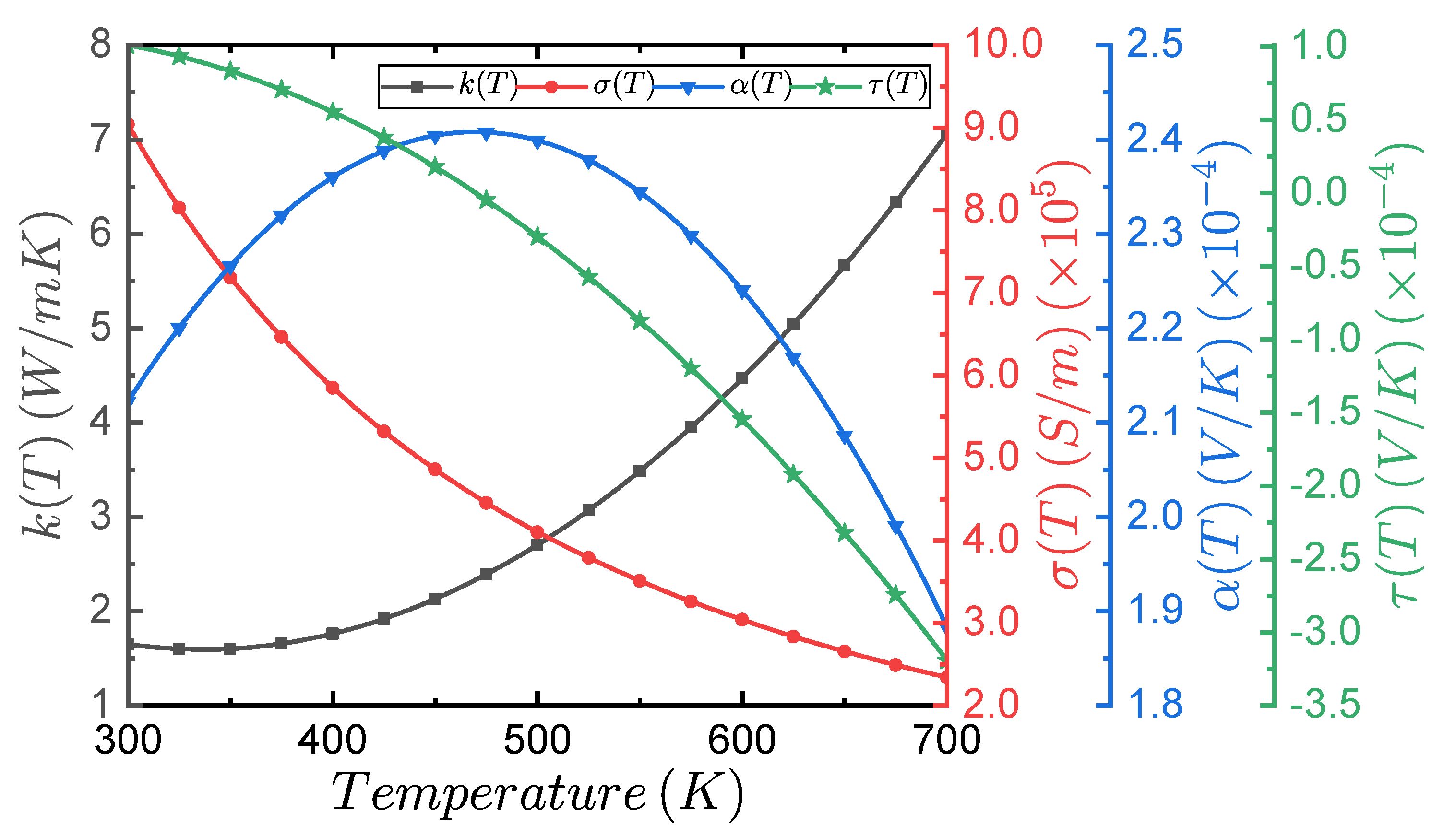
2.1. Thermoelectric Materials and Properties

We used bismuth telluride ${\mathrm{Bi}}_2{\mathrm{Te}}_3$ for the thermoelectric generator (TEG) material. Its properties were considered isotropic and temperature-dependent [26].

Table 1. Geometric parameters of the thermoelectric leg and the temperature-dependent thermoelectric properties of ${\mathrm{Bi}}_2{\mathrm{Te}}_3$ [26].

Parameter	Value/Mathematical Expression	Unit
Cross-sectional area	$A=1.4\times {10}^{-6}$	m${}^2$
Length	$L=1.4\times {10}^{-3}$	m
Thermal conductivity	$\kappa \left(T\right)=\left(0.4131T^2-277.7T+62605\right)\times {10}^{-4}$	W/mK
Electrical conductivity	$\sigma \left(T\right)=\left(0.3927T^2-548.03T+216555\right)\times {10}^{10}$	S/m
Seebeck coefficient	$\alpha \left(T\right)=\left(-0.9905T^2+930.6T+22224\right)\times {10}^{-9}$	V/K
Thomson coefficient	$\tau \left(T\right)=\left(-1.981T^2+9306T\right)\times {10}^{-9}$	V/K

reports the geometric parameter of a single thermoelectric leg, as well as the temperature-dependent thermoelectric properties that are present at an absolute temperature range of $\left(300\le T\le 700\right)$K. The primary geometric parameters are the cross-sectional area A and the length L of the thermoelectric leg. The temperature-dependent thermoelectric properties considered for this study are the thermal conductivity $\kappa \left(T\right)$, the electrical conductivity $\sigma \left(T\right)$, and the Seebeck and Thomson coefficients $\alpha \left(T\right)$, $\tau \left(T\right)$, respectively.

Figure 1 presents the mathematical trend of the temperature-dependent thermoelectric properties shown in Table 1. In the temperature range shown, the only property with an inflection point was $\alpha \left(T\right)$ at $T=475$K, where its slope changed sign, making it decrease, and the Thomson coefficient had a value of $\tau =0$V/K.

2.2. Modeling of Thermoelectric Materials

The numerical simulation was performed using the Thermal-Electric module in the multi-physics software Ansys. According to the Mechanical APDL (Ansys Parametric Design Language) theory reference module [27], the heat flux vector $\overrightarrow{q}$ and the electric current density vector $\overrightarrow{j}$ are the coupled equations that describe the physical behavior of the thermoelectric phenomena. $\overrightarrow{q}$ and $\overrightarrow{j}$ are defined in Equations (1) and (2), respectively.

$$\overrightarrow{q}=T\left[\alpha \right]\overrightarrow{j}-\left[\kappa \right]\nabla T$$

(1)

$$\overrightarrow{j}=\left[\sigma \right]\left(\overrightarrow{E}-\left[\alpha \right]\nabla T\right)$$

(2)

where T is the absolute temperature, $\nabla T$ is the thermal gradient, and $\overrightarrow{E}$ is the electric field. The parameters $\left[\alpha \right]$, $\left[\kappa \right]$, and $\left[\sigma \right]$ are the matrices of the Seebeck coefficient, the thermal conductivity, and the electrical conductivity, as defined by Equations (3), (4), and (5), respectively. The properties matrix relates to the three-dimensional space components $x,y,$ and z.

$$\left[\alpha \right]=\left[\begin{array}{ccc}{\alpha }_{xx}& 0& 0\\ 0& {\alpha }_{yy}& 0\\ 0& 0& {\alpha }_{zz}\end{array}\right]$$

(3)

$$\left[\kappa \right]=\left[\begin{array}{ccc}{\kappa }_{xx}& 0& 0\\ 0& {\kappa }_{yy}& 0\\ 0& 0& {\kappa }_{zz}\end{array}\right]$$

(4)

$$\left[\sigma \right]=\left[\begin{array}{ccc}{\displaystyle \frac{1}{{\rho }_{xx}}}& 0& 0\\ 0& {\displaystyle \frac{1}{{\rho }_{yy}}}& 0\\ 0& 0& {\displaystyle \frac{1}{{\rho }_{zz}}}\end{array}\right]$$

(5)

The Mechanical APDL of Ansys solves multiphysics phenomena for solids via the finite element method (FEM). The equation system applied in the nodes of the representative mesh are the coupled equations for thermoelectricity, as defined by Equation (6). The coupled equation relates to the following terms: $C^t$ is the element-specific heat matrix; $K^T$ is the element diffusion conductivity matrix; Q is the sum of the element heat generation load and element convection surface heat flow vectors; $K^V$ is the element electrical conductivity coefficient matrix; $C^V$ is the element dielectric permittivity coefficient matrix; $K^{Vt}$ is the element Seebeck coefficient coupling matrix; $Q^P$ is the elements Peltier heat load vector; and I is the nodal current load vector. Detailed expressions for the variables in Equation (6) can be found in Appendix A.

$$\left[\begin{array}{cc}\left[C^t\right]& \left[0\right]\\ \left[0\right]& \left[C^V\right]\end{array}\right]\left\{\begin{array}{c}\left\{\dot{T}\right\}\\ \left\{\dot{V}\right\}\end{array}\right\}+\left[\begin{array}{cc}\left[K^t\right]& \left[0\right]\\ [K^{Vt}]& \left[K^v\right]\end{array}\right]\left\{\begin{array}{c}\left\{T\right\}\\ \left\{V\right\}\end{array}\right\}=\left\{\begin{array}{c}\left\{Q\right\}+\{Q^P\}\\ \left\{I\right\}\end{array}\right\}$$

(6)

Figure 2a shows the thermal-electric boundary conditions and the length L of a single thermoelectric leg that was used for the simulation. Regarding the boundary conditions, a Dirichlet thermal boundary condition of constant temperature $T_{hot}=500$K was placed at the heat source surface, along with a fixed current load $I_{load}=1.26$A. On the heat sink surface, a constant thermal boundary condition of temperature $T_{cold}=300$K, and a reference voltage $V_{ref}=0$V were also implemented. For the non-convection case, we defined an adiabatic boundary condition $\dot{Q}=0$W for the side wall of the thermoelectric leg. Additionally, a central dotted line was used to measure the temperature distribution from the heat source to the heat sink along the y-axis. Figure 2b shows the hexahedral mesh used in the simulation and the cross-sectional area A of the leg. The mesh had 31,500 and 135,191 elements and nodes, respectively.

The presented one-dimensional solution was formulated based on the Onsager relationships and the phenomena associated with the cross flux within a thermoelectric leg. An analysis established an energy and species (electrons) balance within the material, whereby critical thermoelectric effects such as Fourier heat conduction, Joule heating, and the Thomson effect were considered. This study was operated under steady-state conditions, thereby implying that the energy storage within the system remained negligible. Additionally, it was postulated that there would be no significant variations in the electrical potential during the operational regime, or, if such variations did occur, they would be sufficiently rapid so as to result in a cumulative charge that approaches zero over time. This equation addresses the traditional methods’ limitations by using an iterative, zero-order homotopy method to solve the coupled differential equations for temperature (Equation (7)) and electrical potential (Equation (8)). This method is a reliable and efficient alternative for solving these equations. The simplified proposed model is represented as follows, where the functions $\kappa \left(T\right)$, $\alpha \left(T\right)$, and $\sigma \left(T\right)$ correspond to the materials’ properties defined by Equations (3)–(5).

$$\begin{array}{c}\hfill \frac{d}{dy}\left[\kappa \left(T\right)\frac{dT}{dy}\right]-jT\frac{d\alpha \left(T\right)}{dT}\frac{dT}{dy}+j^2\sigma \left(T\right)-q_{loss}=0\end{array}$$

(7)

$$\begin{array}{c}\hfill j=\frac{\alpha \left(T\right)}{\sigma \left(T\right)}\frac{dT}{dy}-\frac{1}{\sigma \left(T\right)}\frac{d\varphi }{dy};with\frac{dj}{dt}=0\end{array}$$

(8)

Evaluating the performance of thermoelectric materials and generators is crucial in understanding their potential for energy conversion. One of the key metrics used in this evaluation is conversion efficiency, which can be calculated by determining the ratio of the output power to the input heat. The power generation (P) and thermoelectric efficiency ($\eta$) can be expressed mathematically as follows:

$$P=q_{hot}-q_{cold}-q_{loss}$$

(9)

$$\eta =\frac{P}{q_{hot}}$$

(10)

where $q_H$ and $q_C$ represent the heat supplied to the hot side and the heat removed from the cold side, respectively. $q_{loss}$ represents the heat lost due to factors such as convection and radiation.

The heat flux $q^{″}$ inside any thermoelectric material is the result of both thermal conduction and the heat associated with the electric current crossing through the section area. This can be represented mathematically as follows:

$$q^{″}\left(x\right)=-k\left(T\right)\frac{dT}{dy}+\alpha \left(T\right)jT$$

(11)

where $k\left(T\right)$ is the thermal conductivity, $\alpha \left(T\right)$ is the Seebeck coefficient, j is the current density, and T is the temperature.

The heat supplied to the hot side ($q_{hot}$) and removed from the cold side ($q_{cold}$) can be represented as follows:

$$q_{hot}=q^{″}\left(0\right)$$

(12)

$$q_{cold}=q^{″}\left(L\right)$$

(13)

where L is the length of the thermoelectric material.

$$q_{hot}=-k\left(T_{hot}\right)\frac{dT}{dx}{|}_{y=0}+\alpha \left(T_{hot}\right)j{T}_{hot}$$

(14)

$$q_{cold}=-k\left(T_{cold}\right)\frac{dT}{dx}{|}_{y=L}+\alpha \left(T_{cold}\right)j{T}_{cold}$$

(15)

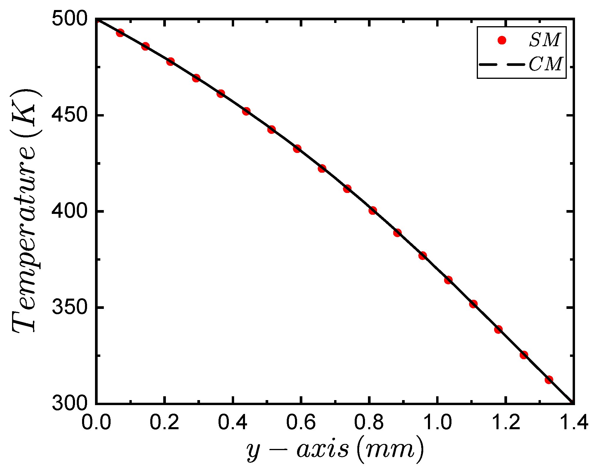
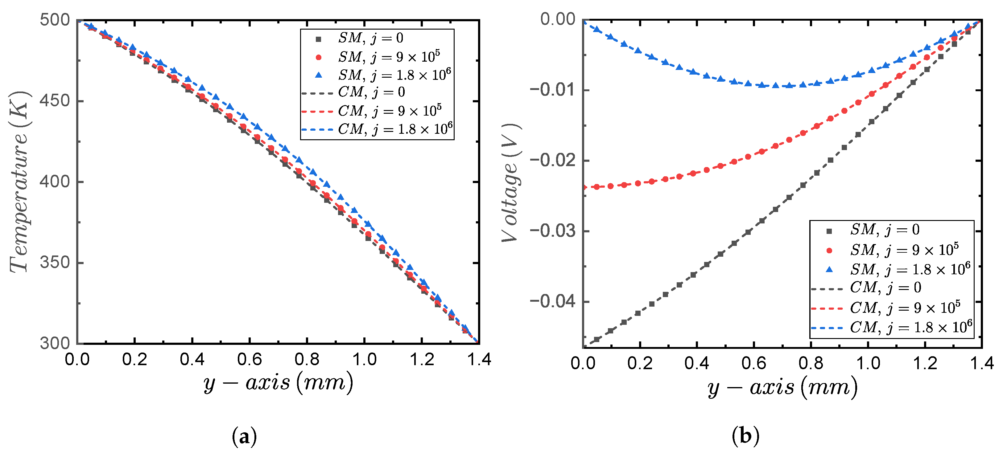
2.3. Comprehensive Model (Ansys) and the Proposed Simplified Model Comparison

Figure 3 presents the comparison between the simplified model (SM) result of the temperature profile of the thermoelectric leg that was reported previously, as well as the complete and comprehensive numerical simulation (CM) that was carried out in this study with Ansys Thermal-Electric. The graph shows the variation in the temperature within a range of $\left(300\le T\le 500\right)$K along the y-axis as a function of the distance d $\left(0\le d\le 1.4\right)$mm. The comparison between the theoretical and numerical profile temperatures showed a good agreement with the relative errors being less than 0.01%. This result validated the numerical procedure for a single thermoelectric leg.

To further validate the simplified model (SM), we compared its temperature and voltage profile results with the comprehensive model’s (CM) results, which was obtained in Ansys Thermal-Electric along the y-axis between a temperature range of $\left(300\le T\le 700\right)$K. The reason for increasing the maximum temperature value to $T=700$K was because of the sudden drop of the Seebeck coefficient $\alpha \left(T\right)$ beyond $T=500$K, as shown in Figure 1. Figure 4a,b present the simplified model (SM) and comprehensive model (CM) temperature and voltage profile results, respectively. These results were developed along the y-axis of the thermoelectric leg (see Figure 2a) within a temperature range of $\left(300\le T\le 500\right)$K and with the current densities of $j=\left(0,9\times {10}^5;1.8\times {10}^6\right)$A/m${}^2$. Figure 4a shows how there was good agreement between the SM and CM model profiles. It can be confirmed that there was a proportional relationship between the rise in temperature due to the increase in current density j caused by the Joule effect. However, the maximum temperature difference between the results for the current densities of $j=0$A/m${}^2$ and $j=1.8\times {10}^{-6}$ was not greater than $9.53$K, which was near the half of the leg length. On the other hand, Figure 4b confirmed the inverse relationship between the generated voltage V and the current load I. In other words, when $j=0$A/m${}^2$, the generated voltage was the so-called “open-circuit voltage $V_{OC}$”, and this was the maximum voltage reachable for a specific thermal difference between the leg boundaries. Also, the generated voltage was at its maximum near the heat source surface, but this decreased to zero ($0$V) near the heat sink surface due to the referenced boundary condition.

Figure 5 presents the temperature and voltage contours that were obtained by the comprehensive (CM) model for a temperature range of $\left(300\le T\le 500\right)$K, which was computed at the coordinate $z=-\sqrt{A}/2$, (see Figure 2b). Figure 5a–c respectively show the temperature contours for the current densities of $j=\left(0,9\times {10}^5,1.8\times {10}^6\right)$A/m${}^2$. The contours show that, for the higher current densities, the isothermal lines for the given temperatures moved toward the heat sink surface. Therefore, the average temperature for the thermoelectric leg increased with the current density (e.g., ${\overline{T}}_{j=0{\mathrm{A}/\mathrm{m}}^2}=409.23$K, ${\overline{T}}_{j=9\times {10}^5{\mathrm{A}/\mathrm{m}}^2}=411.05$K, ${\overline{T}}_{j=1.8\times {10}^6{\mathrm{A}/\mathrm{m}}^2}=415.34$K). Figure 5d–f respectively show the voltage contours for the same current densities. The contour presented in Figure 5d corresponds to the open-circuit case, where the minimum and maximum values of $V_{OC}$ were located at the heat sink and the heat source surfaces, respectively. Figure 5f shows that the maximum values of the voltage shifted towards the center of the leg, thereby setting the heat sink and heat source surfaces with the minimum voltage values; the same results were reached by the solution of the voltage profile when solving the differential one-dimensional equation.

Figure 6a,b present the simplified model (SM) and comprehensive model (CM) temperature and voltage profile results for the boundary conditions of $T_{hot}=700$K and $T_{cold}=300$K, as well as current densities of $j=\left(0,9\times {10}^5,1.8\times {10}^6\right)$A/m${}^2$. Figure 6a shows that there was a good agreement between the SM and CM temperature profiles. In comparison with the temperature curves reported in Figure 4a (with a hot side temperature of 500 K), the maximum temperature difference between the curves for the current densities of $j=0$A/m${}^2$ and $j=1.8\times {10}^{-6}$A/m${}^2$ was not greater than $4.45$K. This means that the increase in current density did not play a significant role in the temperature profile along the y-axis; this could be easily explained considering that the Joule effect has no significant relevance when the thermoelectric leg has high thermal conditions. In Figure 6b, none of the voltage profiles returned to zero; this was in contrast to Figure 4b, where the curve of $j=9\times {10}^{-5}$A/m${}^2$ started and ended at the same value. This can be explained due to $j=9\times {10}^{-5}$A/m${}^2$, which is the current density when the maximum power is generated, as well as due to the fact that this behavior occurs only for that specific value.

Table 2. Temperature $\overline{T}$ and voltage $\overline{V}$ average values of the comprehensive model (CM) results (Figure 5 and Figure 6) for the current densities of $j=\left(0,9\times {10}^5,1.8\times {10}^6\right)$A/m${}^2$, the hot surface temperatures of $T_{hot}=(500,700)$K (which occurred at a constant cold surface temperature of $T_{cold}=300$K).

Current Densities $\mathit{j}$(A/m${}^2$)	Hot Surface Temperature $\left(\mathit{K}\right)$
	${\mathit{T}}_{\mathit{hot}}=\mathbf{500}$		${\mathit{T}}_{\mathit{hot}}=\mathbf{700}$
	$\overline{\mathit{T}}\left(\mathit{K}\right)$	$\overline{\mathit{V}}\left(\mathit{V}\right)$	$\overline{\mathit{T}}\left(\mathit{K}\right)$	$\overline{\mathit{V}}\left(\mathit{V}\right)$
0	$409.23$	$-2.49\times {10}^{-2}$	$554.70$	$-5.86\times {10}^{-2}$
$9\times {10}^5$	$410.82$	$-1.54\times {10}^{-2}$	$554.92$	$-4.30\times {10}^{-2}$
$1.8\times {10}^{-6}$	$415.02$	$-6.03\times {10}^{-3}$	$557.34$	$-2.78\times {10}^{-2}$

summarizes the arithmetic mean of temperature $\overline{T}$ and voltage $\overline{V}$ for the comprehensive model (CM) curves presented in Figure 5 and Figure 6. These values correspond to the hot surface temperatures of $T_{hot}=300$K and $T_{hot}=700$K, the current densities of $j=\left(0,9\times {10}^5,1.8\times {10}^6\right)$A/m${}^2$, and the constant cold surface temperature of $T_{cold}=300$K. The values of ${\overline{T}}_{T_{hot} = 500 \mathrm{K}}$ had less variation than those of ${\overline{T}}_{T_{hot} = 700 \mathrm{K}}$. This was because of the higher temperature differences, which induce larger average temperature changes as the current density increases. Regarding the average voltage values, for both hot surface temperatures of $T_{hot}=500$K and $T_{hot}=700$K, there was a downward trend due to the imposition of a current load, which generated a voltage drop. Additionally, the higher the current density, the larger the variation was for $\overline{V}$ at $T_{hot}=700$K in comparison with its variation at $T_{hot}=500$K. This is due to a larger voltage generation when there was a higher temperature difference between the hot and cold TEG surfaces.

A novel feature of the simplified proposed model (SM) is the ability to model convective heat transfer on the side walls of the solid bodies of the TEG module. Thus, various convective heat transfer coefficients were applied to further compare the SM and the CM results. Three values for the heat transfer coefficient h were used, namely, $h=(10,20,30)$W/m${}^2$K. A constant current density of $j=9\times {10}^5$A/m${}^2$ was imposed. The temperatures of the hot and cold surfaces were $500$K and $300$K, respectively. Figure 7a presents the SM and CM temperature profile results along the y-axis for each variation of h. Similarly, Figure 7b presents the SM and CM voltage profile results along the y-axis for each variation of h. According to these results, both the SM and CM models had a good agreement in modeling temperature and voltage profiles with the wall convective heat transfer. Additionally, the temperature and voltage profiles did not change significantly when a heat transfer coefficient h was applied.

3. Modeling a Complete Thermoelectric Module

We compared the results of the proposed simplified model (SM) with the characteristic curves of the commercial thermoelectric module TEG1-12611-6.0 [28], and to a fully-coupled numerical simulation (comprehensive model—CM) in the Thermal-Electric module of Ansys. The simulations were executed by a 12-core Intel^®, Xeon CPU E5-2667 at 2.90 GHz, and with a 32 GB of RAM workstation. The CAD model was obtained from the commercial TEG module (Section 3.1). Then, a tetrahedral mesh was generated, and a mesh independence study was carried out (Section 3.2). The boundary conditions applied to the numerical simulation were defined (Section 3.3).

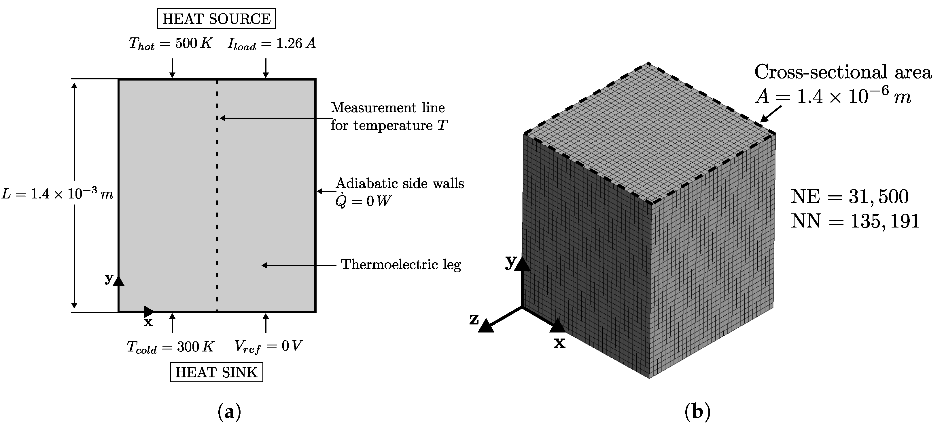
3.1. Thermoelectric Module Geometry

The CAD model for the numerical simulation was obtained in the CAD modeling software SpaceClaim R2022 of Ansys. The CAD model was based on the commercial TEG module TEG1-12611-6.0, which was manufactured by TECTEG MFR. (Ontario, CA, USA) [28]. Figure 8a shows the dimensions of one pair of N- and P-type thermoelectric (TE) materials, which were connected in series by copper electrodes. Each TE leg had two side lengths of $2.4$mm, and a height of $1.3$mm. The copper electrodes were 5.8 mm in length and $2.4$mm in width. The upper and bottom copper electrodes had a height of $0.4$mm and $0.5$mm, respectively. Figure 8b shows the 126-pair-leg TEG module CAD model with its general dimensions. An electrical resistor was connected at the end of the copper electrodes, which acted as an electrical load. The resistor had a cross-sectional area of $A=1.2$mm${}^2$ and a length of $L=73.4$mm. The upper and bottom sides of the TEG module were covered by two graphite rectangles that were $(56\times 56)$mm in length and $1$mm in height. The spacing between the TE legs along the z and x axis was $1$mm. Lastly, in Figure 8b, a top view of the TEG module showing the series connection between the TE legs and the copper electrodes can be seen.

3.2. Boundary Conditions and Parametric Setups

Figure 9 shows the thermal-electric boundary conditions (BCs) used for the TEG module numerical simulation. The thermal BCs, namely the hot $T_{hot}$ and cold $T_{cold}$ temperatures, were placed on the top and bottom surfaces of the graphite material, respectively. Also, an adiabatic thermal condition $\dot{Q}=0$ was assumed for all of the lateral walls of the TEG module, including the copper electrodes, TE legs, and graphite material. Additionally, an electric BC of a zero voltage $V_{ref}=0$ was placed on the vertical surface of the copper electrode, which was connected to an N-type TE leg.

3.2.1. Case 1—The Parametric Setup: Ansys vs. Commercial TEG

To compare the results obtained in the Thermal-Electric module of Ansys with the characteristic curves of the TEG module TEG1-12611-6.0 (manufacturer information), a parametric study was configured in the following manner: firstly, constant hot and cold temperatures of $T_{hot}=573.15$K, and $T_{cold}=303.15$K were used, respectively. Secondly, the voltage reference was maintained as $V_{ref}=0$. Lastly, to simulate an electric load, the resistor’s electrical resistivity ${\rho }_{resistor}$ was varied, as depicted by

Table 3. Variation in the resistor’s electrical resistivity for the parametric studies.

${\mathit{R}}_{\mathit{resistor}}(\Omega )$	${\mathit{\rho }}_{\mathit{resistor}}(\Omega \mathbf{m})$
120,000	1.9619
8	$1.3079\times {10}^{-4}$
6	$9.8093\times {10}^{-5}$
4	$6.5395\times {10}^{-5}$
2	$3.2698\times {10}^{-5}$
1.2	$1.9619\times {10}^{-5}$
1	$1.6349\times {10}^{-5}$
0.8	$1.3079\times {10}^{-5}$
0.6	$9.8093\times {10}^{-6}$
0.4	$6.5395\times {10}^{-6}$
0.2	$3.2698\times {10}^{-6}$
0.09	$1.4714\times {10}^{-6}$
0.07	$1.1444\times {10}^{-6}$
0.05	$8.1744\times {10}^{-7}$
0.03	$4.9046\times {10}^{-7}$
0.01	$1.6349\times {10}^{-7}$

. On one side, the values of ${\rho }_{resistor}$ were varied by assuming an electric resistance from $120$K$\Omega$ to $0.01\Omega$. Then, by using Equation (16), which relates to the geometric and electrical properties of the resistor, ${\rho }_{resistor}$ could be obtained. $A_{resistor}=1.2$mm${}^2$ was the cross-sectional area, $L_{resistor}=73.4$mm was the length, and $R_{resistor}$ was the varied resistance. On the other side, the highest electric resistance was imposed to obtain the open-circuit voltage $V_{OC}$ of the TEG module, and the lowest electric resistance was used to generate the highest current flow through the TEG module.

$${\rho }_{resistor}=\frac{R_{resistor}{A}_{resistor}}{L_{resistor}}$$

(16)

3.2.2. Case 2—The Parametric Setup: Ansys vs. the Proposed Model

To compare the results obtained in the Thermal-Electric module of Ansys with the proposed model, seven temperature differences $\Delta T$ were generated as the thermal loads for the TEG module. First, the cold temperature BC was maintained constant at $T_{cold}=297.95$K, and the voltage reference was held at $V_{ref}=0$. Secondly, the hot temperature BC was varied in a range of $(333.15\le T_{hot}\le 393.15)$K, with steps of $T_{hot,step}=10$K. Lastly, for each temperature difference simulation, the resistor’s electrical resistivity ${\rho }_{resistor}$ was also changed according to the data in Table 3.

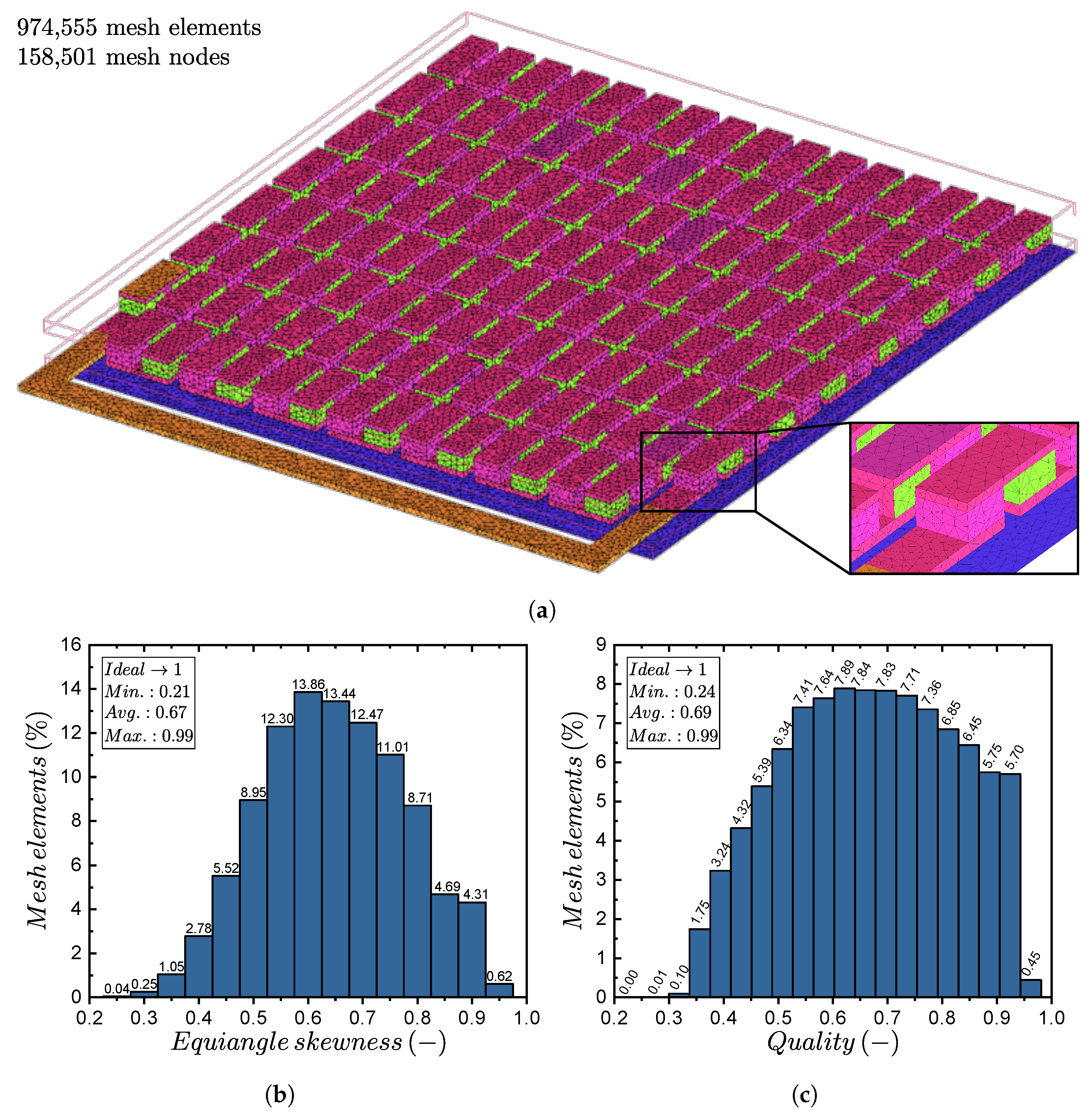
3.3. Mesh Generation

The CAD model mesh was generated in the meshing software ICEM CFD R2022 of Ansys. The mesh presented in the following subsections was a tetrahedral-conformal mesh due to the high number of contacting surfaces between the solid bodies of the CAD model. A conformal mesh is required for the Finite Element Method (FEM) because it allows its nodes to coincide between the contacting surfaces. This permits the iterative solution information to be transferred appropriately between nodes [29]. A mesh independence study, the quality parameters, and the final mesh used in the simulation are also shown.

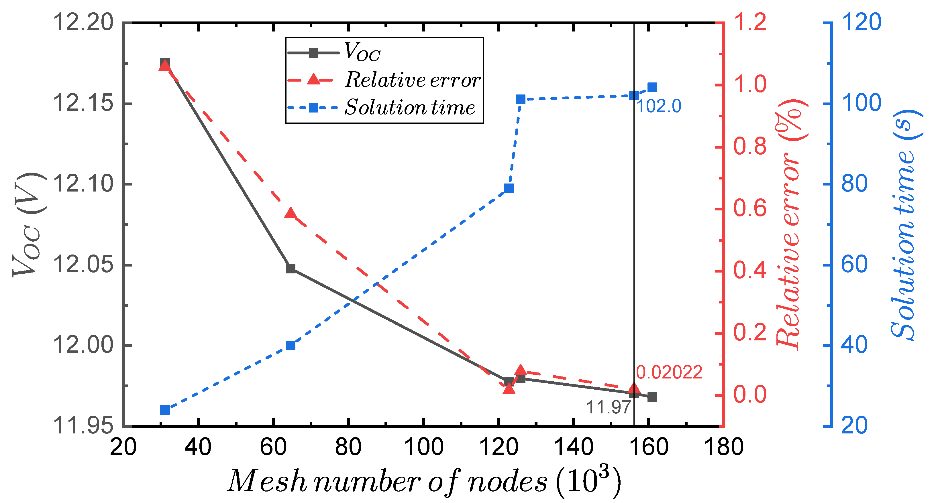
3.3.1. Mesh Independence Study

The mesh independence study considered the open-circuit voltage $V_{OC}$ as the system response quantity (SRQ), i.e., the output value. The parametric simulation for the mesh study had constant hot and cold temperature values of $T_{hot}=573.15$K and $T_{cold}=303.15$K as input values, respectively. The mesh was globally refined by reducing the maximum element size in ICEM CFD. Figure 10 shows, as a function of the mesh number of nodes, the values of $V_{OC}$, the relative error between each refinement point, and the simulation time. The $V_{OC}$ and relative error curve trends showed that the SRQ value tends to be fixed as the mesh becomes more refined. Additionally, the simulation time increased rapidly to around 120,000 mesh nodes. Then, it tended to be constant near 100 s. According to the mesh study, we selected a mesh composed of 158,501 nodes. This is because we considered the relative error to be low enough to continue the simulation with the values shown by the vertical line that represented the characteristic values of the chosen mesh. These values corresponded to $V_{OC}=11.97$V, a relative error of 0.02022%, and a solution time of 102 s.

3.3.2. Final Mesh

Figure 11a shows the final mesh used for the simulations of this section. The mesh was made up of tetrahedral-conformal-type elements that were generated in the ICEM CFD of Ansys with 974,555 elements and 158,501 nodes. ICEM CFD offers advanced mesh acquisition and diagnostic capabilities for applications like computational fluid dynamics but also for structural and thermal analysis. It facilitates the creation of mesh output files that are compatible with various structural solvers, such as Ansys Mechanical APDL, Autodyn, LS-DYNA, ABAQUS, and NASTRAN [30]. The distinction between the mesh for a single TEG leg (Figure 2b) and a complete TEG module (Figure 11a) was the mesh topology sharing. When a topology is shared between distinct geometry surfaces, the mesh nodes match between them. This is crucial for the accurate transfer of mesh information between contacting surfaces [27], thus resulting in the prevention of additional numerical errors. Meshing with a shared topology is notably more complex for a complete TEG module when compared to a single TEG leg due to the increased number of contacting surfaces; therefore, this poses a challenge when meshing a TEG module. As a result, opting for tetrahedral mesh elements becomes a more viable approach than using hexahedral elements because of its adaptability without compromising the mesh quality. While we initially attempted to utilize Ansys’s Mesh module to generate a shared topology mesh for the complete TEG module, it fell short of achieving acceptable quality metrics. Conversely, ICEM CFD successfully produced the desired mesh, even at a lower computational cost.

Figure 11b shows the mesh element equiangular skewness, in which the value 1 represents an ideal mesh element, while 0 represents a bad quality element. On the one hand, 0.001% of the total mesh elements had a minimum value of 0.21, while 0.61% of the total elements had a maximum value of 0.99. On the other hand, the average value was 0.67. This quality parameter cannot be lower than 0.05 for the Mechanical APDL solver [27]. Figure 11c shows the number of the elements’ percentage distribution as a function of the quality parameter. Values closer to 1 represent the ideal mesh element, while values closer to 0 represent the worst. The minimum value was 0.24, and this was present in 0.002% of the total mesh elements. The maximum value was 0.99 for 0.44% of the total elements, while the average value was 0.69. According to the quality parameter distributions, the mesh accomplished the minimum solver requirement for avoid floating points during the solution process. Additionally, the mesh can be considered good quality due to the low percentage of bad elements and the average values that were close to the ideal quality parameter value.

4. Results

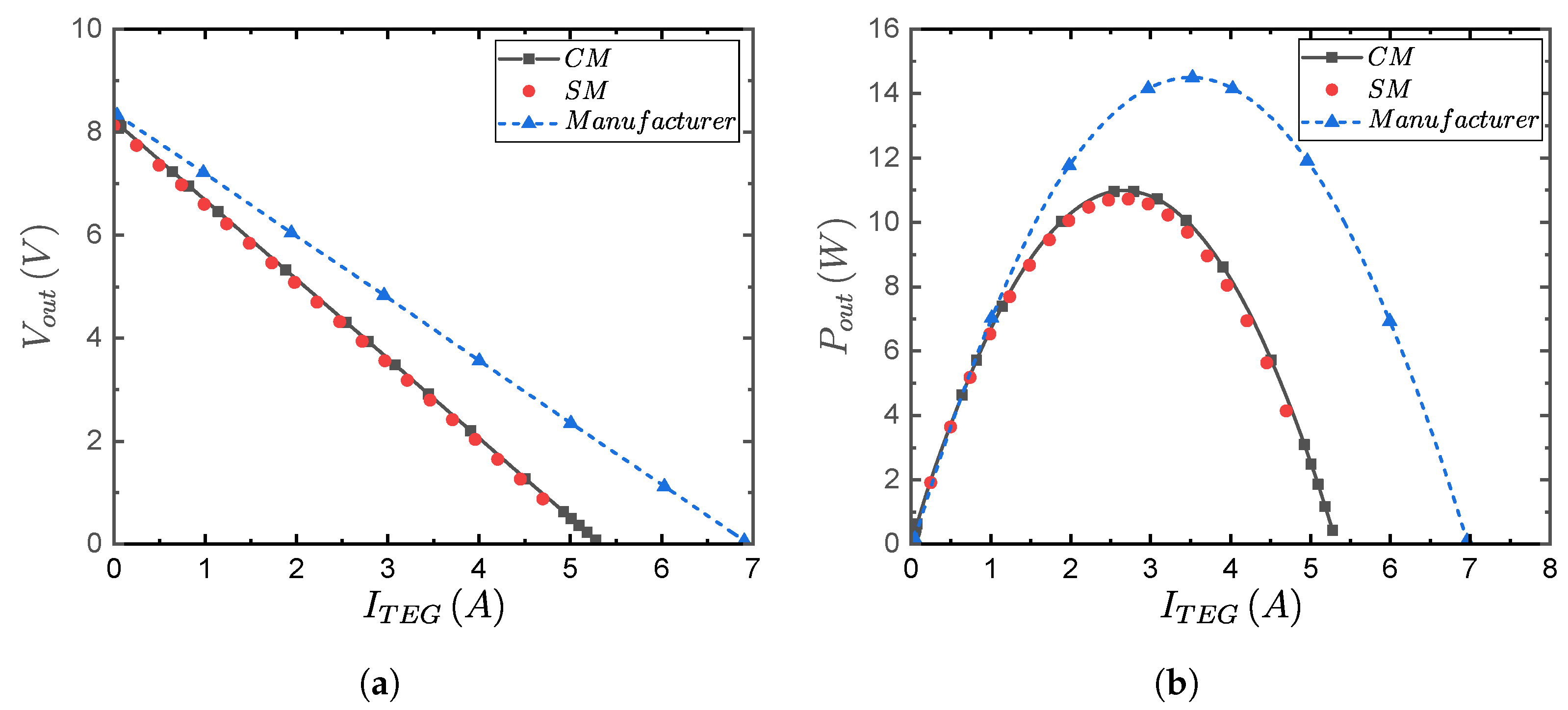
4.1. Case 1 Results: Ansys vs. Commercial TEG

Figure 12 shows the result comparison obtained by the comprehensive model (CM) when using Ansys Thermal-Electric, the simplified proposed model (CM) and the commercial TEG module’s characteristic curves (manufacturer information) were at a fixed temperature difference $\Delta T$. These results were obtained for the thermal BCs of $T_{hot}=573.15$K and $T_{cold}=303.15$K, which generated a temperature difference of $\Delta T=270$K (see Section 3.2.1 for the parametric study details). Figure 12a,b show the TEG module’s output voltage $V_{out}$ and output power $P_{out}$ as functions of the TEG module current $I_{TEG}$. Regarding the voltage trends, the open-circuit voltage $V_{OC}$ was obtained at the highest imposed electrical resistivity ${\rho }_{resistor}$, which generated no current flow $I_{TEG}$ through the TEG module. Additionally, due to Ohm’s law, the lower the resistor’s electrical resistivity ${\rho }_{resistor}$, the higher the TEG current $I_{TEG}$. Similarly, the inverse relationship between $V_{out}$ and $I_{TEG}$ was because there was a series connection between the TEG module´s internal electrical resistance and the external electrical load, thereby resulting in a voltage divider circuit. For this circuit, the input voltage was $V_{OC}$, which becomes divided according to the two aforementioned electrical resistances’ ratios. As for the output power, it was calculated as $P_{out}=I_{TEG}{V}_{out}$, which generated a concave downward trend with a peak value.

Concerning the results, there were good agreements between the SM and CM model results for both $V_{out}$ and $P_{out}$. However, the characteristic curves of output voltage and power of the TEG module’s manufacturer information were higher than those obtained by the SM and the CM models. The magnitude discrepancies between the unmatched curves were the following: the range of the TEG current for the CM model’s results was $(0\le I_{TEG}\le 5.3)A$; whereas, for the manufacturer information, it was $(0\le I_{TEG}\le 7)A$. This means there was a relative error between the $I_{TEG}$ maximum values in the SM and CM with respect to the manufacturer report of 24.3%. Regarding the output voltage lines obtained in Ansys and the proposed model, there was a relative error between its slopes of 0.3%. Concerning the output power $P_{out}$, there was an average relative error between the SM and the CM models curves of 0.1%. Furthermore, when comparing the voltage and power results for the CM and SM models, we found that the relative errors between the models were below 7%, which is an acceptable error and serves to validate the simplified proposed model (SM). The reason for the described discrepancies was the undisclosed physical dimensions and the thermoelectric material properties of the commercial TEG module (TEG1-12611-6), which was used as a reference for the present study. As a result, the commercial TEG module had to undergo reverse engineering to determine the approximate physical dimensions. However, this process is destructive, thus requiring the module to be opened and damaged. Similarly, the thermoelectric properties used for the simulations were obtained from the TEG module manufacturer (TECTEG MFR., [28]). However, there was no certainty that they were precisely the material properties of the TEG module used to obtain the characteristic curves of the manufacturer information. Thus, we believe these reasons were the cause for the discrepancies seen in Figure 12a,b between the comprehensive model and the manufacturer information.

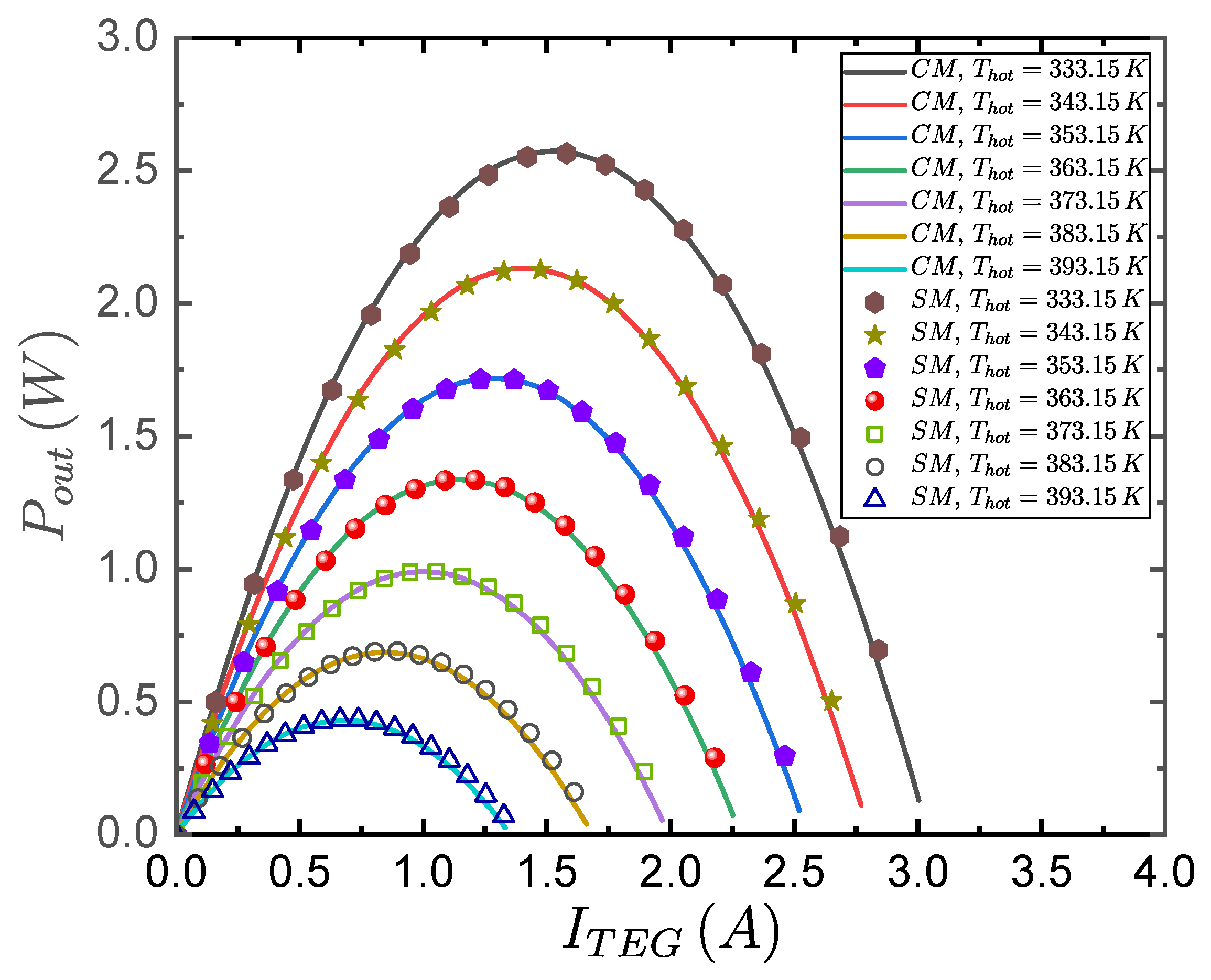
4.2. Case 2 Results: Ansys vs. the Proposed Model and Model Tuning

At the interface between the cool and hot sides of the TEG module and the semiconductor material, the electrical current flow through the junction lead to the generation of Peltier heat, conduction heat transfer, and Joule heating. Figure 13 shows the total heat flux contour detail of the complete TEG model that was obtained with the comprehensive model (Ansys Thermal-Electric). The figure shows that there was a non-uniform heat flux concentration at the TEG module’s corners and junctions, whose magnitude depends on the current density flowing through the body solids. The maximum total heat flux value on these adjacent edges was as high as 8.29 $\times {10}^5$W/m${}^2$, while the average value for the complete TEG module was around 61,429 W/m${}^2$. These high values of the model’s edges can affect the comparison between the comprehensive and proposed models. These sorts of phenomena are not considered in the proposed simplified model due to its one-dimensional conception. Equations (17) and (18) describe the heat transfer for the hot and cold sides, respectively.

$$-I{\alpha }_P{T}_P{{|}_{x=0}+I{\alpha }_N{T}_N|}_{x=0}+\frac{I^{2}R}{2}=-k_P{A}_P\frac{\partial T_P}{\partial x}{|}_{x=0}-k_N{A}_N\frac{\partial T_N}{\partial x}{|}_{x=0}$$

(17)

$$-I{\alpha }_P{T}_P{{|}_{x=L}+I{\alpha }_N{T}_N|}_{x=L}+\frac{I^{2}R}{2}=-\left(-k_P{A}_P\frac{\partial T_P}{\partial x}{|}_{x=L}-k_N{A}_N\frac{\partial T_N}{\partial x}{|}_{x=L}\right)$$

(18)

Although the simplified model was accurate for a single thermoelectric element, extending a single model for the entire module is complex. Phenomena such as electric charge accumulation, heat losses due to conduction, convection, and radiation are present in all elements. In addition, the electric and thermal interaction can occur with the filler, as well as upper and lower plates junctions. Moreover, the effects of pressure and contact gaps that allow for air layers (insulation), contact resistance, the thermal resistance caused by the thermal paste, and the impact of thermal mismatching were determined. These generated the differences between the electrical generation of a single pair and the generation of a complete module with hundreds of pairs. Therefore, it is important to be able to modify the simplified model with TE variable properties, which was developed for a single TE element by adjusting two proposed parameters. As a methodology for this tuning, two new model parameters were introduced: an equivalent effective area factor $\left(F_A\right)$, and a power factor parameter ($F_P$) for the total power generation.

$$A_f=F_{A}A$$

(19)

where $A_f$ is the equivalent effective area of the legs of the entire module, and A is the cross-section area of a single TE leg.

The power generation P was computed as follows:

$$P=F_P(P_{n-type}+P_{p-type})$$

(20)

This approach allowed for the extension of the simplified model’s results for a single TE couple to the entire module, and this was achieved without computing all the physical phenomena involved in an actual module. To estimate the model parameters, there were multiple algorithmic techniques that were previously studied [31]. In this work, a continuous genetic algorithm (CGA) was implemented to find $F_A$ and $F_P$ from a single operation curve that was obtained with the comprehensive model simulated in Ansys (Figure 12).

The two parameters of the proposed model were tuned with a single operating curve (for the given temperature differences $T_{hot}$ and $T_{cold}$); subsequently, a comparison was carried out between the results obtained by the comprehensive model (CM) and the tuned simplified proposed model (SM) with the calculated parameters for different temperature differences. Figure 14 presents the results obtained by the comprehensive model (CM) of Ansys and the results after the tuning of the simplified proposed model (SM). The parametric study setup was described in Section 3.2.2. The figure shows the output power $P_{out}$ for seven temperature differences $\Delta T$, which varied in only the hot side temperature $T_{hot}$ with a fixed $T_{cold}=295.95$ K. There was a good agreement between the comprehensive (CM) and simplified model (SM) in the power delivered from the TEG module under different temperature conditions. At the highest $\Delta T=95.2$K, the maximum TEG module current was $I_{TEG}=3$A, for a maximum power output of $P_{out}=2.57$W. The equivalent effective area factor $\left(F_A\right)=0.86$ and the power factor parameter $F_P=1.12$ were found after 100 times with 50 individuals for a population size and a CGA stop criteria of 1000 iterations, or a root mean square error of $1\times {10}^{-6}$ W.

It is worth noting that the proposed method shows a good agreement with the commercial software results for a wide range of temperature differences, thereby indicating its validity and reliability in predicting the performance of a TEM. Further improvements to the model could be achieved by considering more complex interactions between coupling materials and TE, as well as by including other effects such as the presence of contact resistances and the influence of heat losses by radiation. Overall, the proposed model provides a useful tool for optimizing the design of thermometric systems and devices, thereby enabling a more accurate and efficient utilization of this eco-friendly energy conversion technology [32].

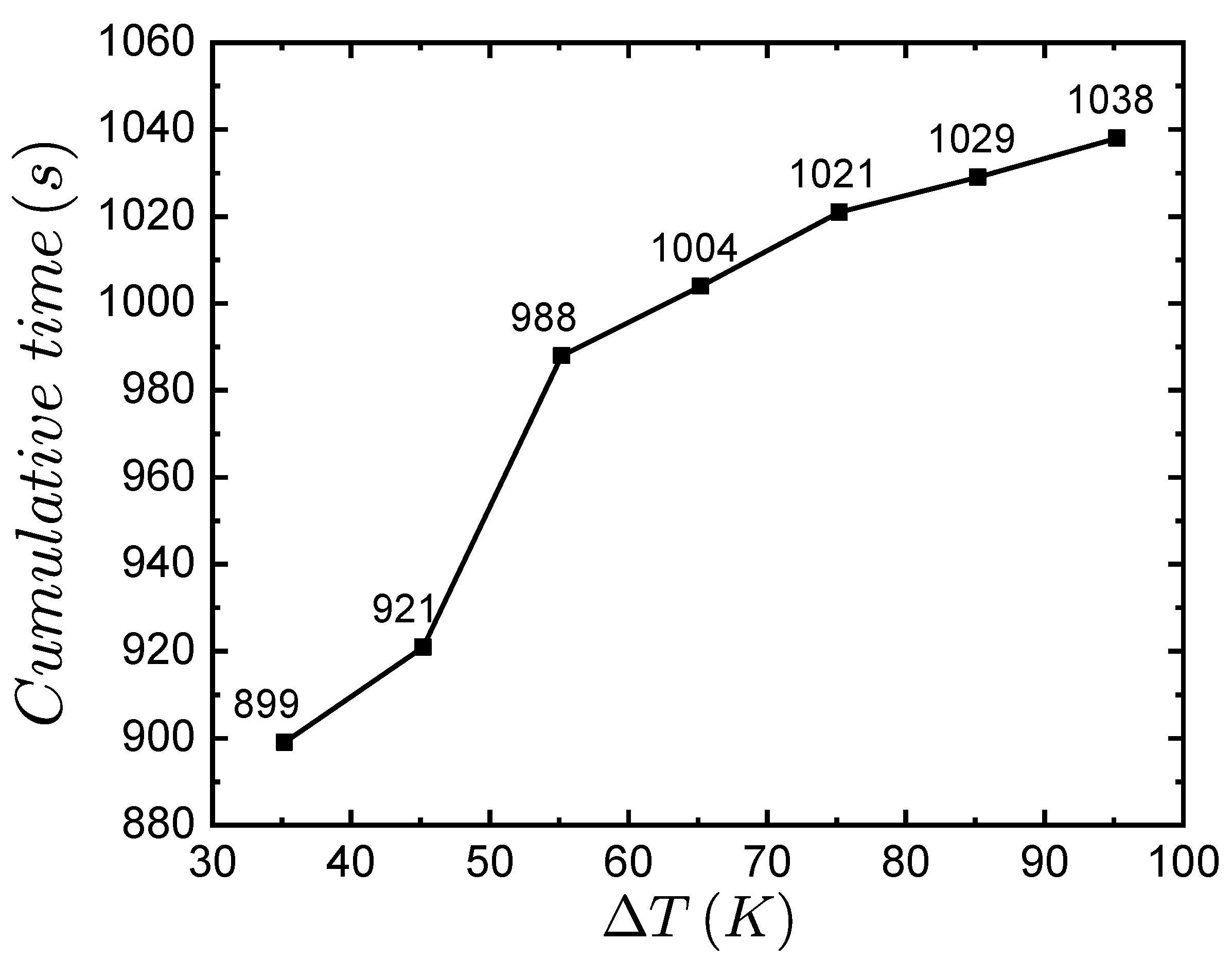
4.3. Simulation Time Analysis for a Parametric Study of a Thermoelectric Generator Module

Table 4. Mesh and parametric study on the cumulative and total time required report.

	Simulation Time for Different $\Delta \mathit{T}$ Varying ${\mathit{\rho }}_{\mathit{resistor}}$ (See Table 3)
	$\Delta \mathit{T}=\mathbf{35.2}$K (s)	$\Delta \mathit{T}=\mathbf{45.2}$K (s)	$\Delta \mathit{T}=\mathbf{55.2}$K (s)	$\Delta \mathit{T}=\mathbf{65.2}$K (s)	$\Delta \mathit{T}=\mathbf{75.2}$K (s)	$\Delta \mathit{T}=\mathbf{85.2}$K (s)	$\Delta \mathit{T}=\mathbf{95.2}$K (s)
	61	63	63	68	71	61	84
	54	60	69	60	60	62	65
	52	58	61	60	63	61	59
	52	57	63	65	64	64	64
	54	62	64	65	62	61	62
	56	64	54	60	65	59	63
	65	57	59	62	71	69	65
	58	56	58	68	62	64	65
	60	54	62	65	60	65	63
	55	56	63	61	63	60	66
	54	55	61	63	64	65	65
	55	52	62	60	64	62	59
	57	54	66	60	61	62	63
	54	52	63	64	63	62	69
	58	60	60	60	64	67	63
	54	61	60	63	64	85	63
Mean $\overline{t}$ (s)	56.19	57.56	61.75	62.75	63.81	64.31	64.88
Stand. dev. ${\sigma }_x$ (s)	3.51	3.78	3.38	2.84	3.17	6.11	5.66
Total time ∑ (h)	$t_{total}=t_{mesh}+t_{par.,study}=2.04$h

presents the results of a parametric study that was performed on a single TEG module consisting of 126 thermoelectric pairs. The simulations were carried out using a 12-core Intel^® Xeon CPU E5-2667 that was clocked at 2.90 GHz, and 32 GB of a RAM workstation. The total simulation time for the parametric study included the cumulative time sum of the mesh study, which comprised six refinement levels (see Figure 10). Additionally, the simulation time depended on the parametric study, which considered 7 different $\Delta T$ values and 16 ${\rho }_{resistor}$ variations.

The simulation time for the comprehensive model (CM) varied with changes in $\Delta T$ and ${\rho }_{resistor}$. For each combination, the simulation time exhibited oscillations with respect to ${\rho }_{resistor}$, but these were monotonically increased as $\Delta T$ increased (see Figure 15). For a change of $\Delta T=60$ K, the simulation time increased by 139 s. The total simulation time for the entire parametric study of the single TEG module was approximately 2.04 h. Therefore, if a parametric study required running simulations on multiple TEG modules, either in series or parallel, the total simulation time would increase significantly.

Additionally, the mean simulation time and the standard deviation for each $\Delta T$ value were also reported, along with the total simulation time for the mesh and parametric study. From the table, we can see that the simulation time generally increased as the time step $\Delta T$ increased. This makes sense since a larger time step requires fewer calculations, which results in faster simulations. However, we can also see that the simulation time was affected by the resistor density ${\rho }_{resistor}$, with some combinations resulting in longer simulation times than others. The results show that the mean simulation time increases with the temperature interval, which ranged from 56.19 s for $\Delta T=35.2$ K to 64.88 s for $\Delta T=95.2$ K. The standard deviation also varied for each temperature interval, and these ranged from 2.84 s to 6.11 s. The total time for the study, including meshing and parametric analysis, was reported to be 2.04 h. These findings suggest that the increase in temperature interval leads to an increase in simulation time, with higher variability found at higher temperatures. Therefore, a careful selection of temperature intervals for the parametric study was required to optimize the simulation time while maintaining an acceptable level of accuracy. Furthermore, the reported total time for the study may be useful for project planning and resource allocation.

Finally, the total simulation time for the mesh and parametric study was reported as $t_{total}=t_{mesh}+t_{par.,study}=2.04$ h. This provided an overall measure of the computational cost of the study, and it can be used to evaluate the efficiency of the simulation setup. Conversely, it also required a significant computational effort, whereby it took, on average, 63 s per simulation to obtain results for a specific current and temperature differential. The use of a simple model instead of an Ansys simulation can be highly beneficial in large scale situations. Although the full model provides an accurate solution, it requires a significant computational effort, which can be time-consuming and expensive. In contrast, a simplified model can offer comparable results at a fraction of the computational cost (1.1 s). In industrial applications where the analysis of many TEG modules is required, the reduced accuracy of the simplified model is outweighed by the much faster computational time. Moreover, a simplified model can help in identifying the key variables that affect the performance of the system, which can thus provide useful insights that can guide further optimization efforts. Therefore, the use of a simple model can provide a practical and efficient solution for many engineering applications.

5. Conclusions

This study aimed to address the challenge of low energy conversion efficiency in thermoelectric generators by developing a methodology that considers temperature-dependent material properties and convection heat losses. The proposed model for the analysis of TEGs leads to a higher accuracy than previous models by considering the convection heat losses at the thermoelectric legs and the two parameters required to predict the power output behavior for a complete module.

The results obtained from our proposed method were subjected to rigorous comparison and validation: first, against a single thermoelectric leg. Remarkably, the relative errors between the outcomes of the proposed model and the comprehensive model (Ansys) were found to be less than 0.01%. We extended our analysis to encompass the thermoelectric characterization of a complete commercial module that consisted of 126 thermoelectric pairs. In this larger-scale evaluation, the proposed model continued to demonstrate its efficacy, yielding relative errors of less than 7% when compared to the results generated by the comprehensive model. This successful prediction reaffirmed the robustness and accuracy of our proposed model in simulating complex thermoelectric systems.

To further validate our proposed simplified model, we compared its results with those of the comprehensive model through a fully coupled thermoelectric simulation using the Finite Element Method, which was applied to a complete thermoelectric module. The relative error observed in the slope of the voltage linear trends between the SM and CM was 0.3%. Several factors contributed to this discrepancy. Firstly, the manufacturer did not disclose the critical physical dimensions and thermoelectric material properties of the commercial TEG module. Consequently, we used reversed engineering techniques to approximate these parameters, and this inherently introduced some uncertainty into the model. Secondly, the one-dimensional nature of our proposed model did not account for non-uniform heat flux concentrations. These concentrations were primarily located at 90-degree adjacent edges, and they exhibited peak values as high as $8.29\times {10}^5$ W/m${}^2$. These values significantly deviated from the average heat flux of 61,429 W/m${}^2$. This non-uniform heat distribution further contributed to the observed variations between our model and the comprehensive model. Despite these challenges, it is worth noting that the characteristic curves generated by our proposed model remained as acceptable predictions for the TEG module in question, even when considering the inherent limitations of it being a one-dimensional model.

The one-dimensional proposed model can be a better choice for characterizing a TEG module because of it simulation times. On the one hand, if we were to quantify the computational cost it takes to simulate a complete TEG module by means of FEM methods, as was carried out in the comprehensive model (Ansys), we found that it would take a total time of 2.04 h to complete the study. This includes the consideration of the meshing and simulation waiting times. On the other hand, the proposed model can resolve the complete TEG module in only 1.1 s, which is approximately 8000 times faster compared to the comprehensive model. We also found that the time required to achieve a solution with the comprehensive model increased in proportion to the temperature difference between the hot and cold surfaces of the TEG module. This implies that the FEM methods might not be the better choice for applications where high-temperature differences are applied due to the increasing simulation times. Therefore, for industrial applications where the analysis of many TEG modules is required, the reduced accuracy of the simplified model is outweighed by the much faster computational time.

This study provides a deeper understanding of the thermoelectric energy conversion process, as well as offers guidance for designing and optimizing thermoelectric generators for practical applications. Additionally, it is important to take into account the potential challenges in practical engineering such as convection heat losses at the legs of TEGs, which can significantly impact energy conversion efficiency. Overall, thermoelectric generators play a crucial role in sustainable energy development due to their energy conversion capabilities and advantages over other conventional methods. This research fills a gap in the field by providing a solution that addresses the limitations of previous models and increases the accuracy of TEG analysis. While this study has made significant strides in improving the accuracy of thermoelectric generator (TEG) analysis, there remains avenues for further research and development in this field. One potential area of future work involves refining the one-dimensional model to account for non-uniform heat flux concentrations, as observed in practical TEG modules. Incorporating a more comprehensive treatment of these non-uniformities can lead to even more accurate predictions, and it can enhance the model’s applicability to a wider range of TEG designs. In terms of computational efficiency, further research could focus on optimizing the Finite Element Method (FEM) simulations used in comprehensive models. Developing techniques to reduce the computational time, especially for cases with high-temperature differences, would be invaluable for practical engineering applications. Additionally, investigating the model’s performance and accuracy under varying operational conditions and materials can provide insights into its robustness and limitations.

References

1. Wang, Z.-L.; Funada, T.; Onda, T.; Chen, Z.-C. Knowledge extraction and performance improvement of bi 2 te 3-based thermoelectric materials by machine learning. Mater. Today Phys. 2023, 31, 100971. [Google Scholar] [CrossRef]
2. Wei, J.; Zhou, Y.; Wang, Y.; Miao, Z.; Guo, Y.; Zhang, H.; Li, X.; Wang, Z.; Shi, Z. A large-sized thermoelectric module composed of cement-based composite blocks for pavement energy harvesting and surface temperature reducing. Energy 2023, 265, 126398. [Google Scholar] [CrossRef]
3. Gürbüz, H.; Akçay, H.; Topalcı, Ü. Experimental investigation of a novel thermoelectric generator design for exhaust waste heat recovery in a gas-fueled si engine. Appl. Therm. Eng. 2022, 216, 119122. [Google Scholar] [CrossRef]
4. Luo, D.; Wang, R.; Yan, Y.; Yu, W.; Zhou, W. Transient numerical modelling of a thermoelectric generator system used for automotive exhaust waste heat recovery. Appl. Energy 2021, 297, 117151. [Google Scholar] [CrossRef]
5. Liu, Y.; Zhang, Y.; Xiang, Q.; Hao, F.; An, Q.; Chen, H. Comprehensive modeling and parametric analysis of multi-mission radioisotope thermoelectric generator. Appl. Therm. Eng. 2022, 219, 119447. [Google Scholar] [CrossRef]
6. Sanin-Villa, D.; Monsalve-Cifuentes, O.D.; Rio, J.S.D. Early fever detection on covid-19 infection using thermoelectric module generators. International J. Electr. Comput. Eng. (IJECE) 2021, 11, 3828–3837. [Google Scholar] [CrossRef]
7. Sargolzaeiaval, Y.; Ramesh, V.P.; Ozturk, M.C. A comprehensive analytical model for thermoelectric body heat harvesting incorporating the impact of human metabolism and physical activity. Appl. Energy 2022, 324, 119738. [Google Scholar] [CrossRef]
8. Sanin-Villa, D. Recent developments in thermoelectric generation: A review. Sustainability 2022, 14, 16821. [Google Scholar] [CrossRef]
9. Zhang, M.; Tian, Y.; Xie, H.; Wu, Z.; Wang, Y. Influence of thomson effect on the thermoelectric generator. Int. J. Heat Mass Transf. 2019, 137, 1183–1190. [Google Scholar] [CrossRef]
10. Lan, Y.; Lu, J.; Li, J.; Wang, S. Effects of temperature-dependent thermal properties and the side leg heat dissipation on the performance of the thermoelectric generator. Energy 2021, 243, 123035. [Google Scholar] [CrossRef]
11. Guo, X.; Zhang, H.; Yuan, J.; Wang, J.; Zhao, J.; Wang, F.; Hou, S. Energetic and exergetic analyses of a combined system consisting of a high-temperature polymer electrolyte membrane fuel cell and a thermoelectric generator with thomson effect. Int. J. Hydrogen. Energy 2019, 44, 16918–16932. [Google Scholar] [CrossRef]
12. Sun, Y.; Chen, G.; Duan, B.; Li, G.; Zhai, P. An annular thermoelectric couple analytical model by considering temperature-dependent material properties and thomson effect. Energy 2019, 187, 115922. [Google Scholar] [CrossRef]
13. Yamashita, O. Effect of linear and non-linear components in the temperature dependences of thermoelectric properties on the energy conversion efficiency. Energy Convers. Manag. 2009, 50, 1968–1975. [Google Scholar] [CrossRef]
14. Chen, W.-H.; Huang, T.-H.; Augusto, G.L.; Lamba, R.; Maduabuchi, C.; Saw, L.H. Power generation and thermal stress characterization of thermoelectric modules with different unileg couples by recovering vehicle waste heat. J. Clean. Prod. 2022, 375, 133987. [Google Scholar] [CrossRef]
15. Cui, Y.J.; Wang, B.L.; Wang, P. Analysis of thermally induced delamination and buckling of thin-film thermoelectric generators made up of pn-junctions. Int. J. Mech. Sci. 2017, 149, 393–401. [Google Scholar] [CrossRef]
16. Cui, Y.J.; Wang, B.L.; Wang, K.F.; Wang, G.G.; Zhang, A.B. An analytical model to evaluate the fatigue crack effects on the hybrid photovoltaic-thermoelectric device. Renew. Energy 2021, 182, 923–933. [Google Scholar] [CrossRef]
17. Sanin-Villa, D.; Monsalve-Cifuentes, O.D.; Henao-Bravo, E.E. Evaluation of thermoelectric generators under mismatching conditions. Energies 2021, 14, 8016. [Google Scholar] [CrossRef]
18. Rogl, G.; Garmroudi, F.; Riss, A.; Yan, X.; Sereni, J.G.; Bauer, E.; Rogl, P. Understanding thermal and electronic transport in high-performance thermoelectric skutterudites. Intermetallics 2022, 146, 107567. [Google Scholar] [CrossRef]
19. Vijay, V.; Harish, S.; Archana, J.; Navaneethan, M. Realization of an ultra-low lattice thermal conductivity in bi2agxse3 nano-structures for enhanced thermoelectric performance. J. Colloid Interface Sci. 2023, 637, 340–353. [Google Scholar] [CrossRef]
20. Wee, D. Analysis of thermoelectric energy conversion efficiency with linear and nonlinear temperature dependence in material properties. Energy Convers. Manag. 2011, 52, 3383–3390. [Google Scholar] [CrossRef]
21. Ju, C.; Dui, G.; Zheng, H.H.; Xin, L. Revisiting the temperature dependence in material properties and performance of thermoelectric materials. Energy 2017, 124, 249–257. [Google Scholar] [CrossRef]
22. Wang, P.; Wang, K.F.; Wang, B.L.; Cui, Y.J. Modeling of thermoelectric generators with effects of side surface heat convection and temperature dependence of material properties. Int. J. Heat Mass Transf. 2019, 133, 1145–1153. [Google Scholar] [CrossRef]
23. Wielgosz, S.E.; Clifford, C.E.; Yu, K.; Barry, M.M. Fully-coupled thermal-electric modeling of thermoelectric generators. Energy 2023, 266, 126324. [Google Scholar] [CrossRef]
24. Sreekala, P.; Ramkumar, A.; Rajesh, K. Enhancing the defense application with Ansys model of thermoelectric generation for coil gun. Sustain. Energy Technol. Assess. 2022, 54, 102806. [Google Scholar] [CrossRef]
25. Bhuiyan, M.S.R.; El-Shahat, A.; Soloiu, V. Thermoelectric generator analysis through Ansys and matlab/simulink. In Proceedings of the IEEE SoutheastCon 2019, Huntsville, AL, USA, 11–14 April 2019. [Google Scholar] [CrossRef]
26. Fraisse, G.; Ramousse, J.; Sgorlon, D.; Goupil, C. Comparison of different modeling approaches for thermoelectric elements. Energy Convers. Manag. 2013, 65, 351–356. [Google Scholar] [CrossRef]
27. Ansys Inc. Theory Reference for the Mechanical APDL and Mechanical Applications; Ansys Inc.: Canonsburg, PA, USA, 2023. [Google Scholar]
28. TECTEG MFR. Division of Thermal Electronics Corporation. Specifications TEG Module TEG1-12611-6.0. 2022. Available online: https://tecteg.com/wp-content/uploads/2014/09/SpecTEG1-12611-6.0TEG-POWERGENERATOR-new.pdf (accessed on 10 October 2022).
29. Nicolas, G.; Fouquet, T. Adaptive mesh refinement for conformal hexahedralmeshes. Finite Elem. Anal. Des. 2013, 67, 1–12. [Google Scholar] [CrossRef]
30. Ansys Inc. Ansys ICEM CFD User’s Manual; Ansys Inc.: Canonsburg, PA, USA, 2023. [Google Scholar]
31. Sanin-Villa, D.; Montoya, O.D. Grisales-Noreña, L.F. Material property characterization and parameter estimation of thermoelectric generator by using a master–slave strategy based on metaheuristics techniques. Mathematics 2023, 11, 1326. [Google Scholar] [CrossRef]
32. Sanin-Villa, D.; Henao-Bravo, E.; Ramos-Paja, C.; Chejne, F. Evaluation of power harvesting on dc-dc converters to extract the maximum power output from tegs arrays under mismatching conditions. J. Oper. Autom. Power Eng. 2023; in press. [Google Scholar] [CrossRef]
Figure 1. Temperature dependence of the thermoelectric properties of Bi 2 Te 3 .
Energies 16 07082 g001
Figure 2. Numerical model of a single thermoelectric leg that was used in the simulation. (a) A 2D view of the leg showing the geometric parameters and the thermoelectric boundary conditions. (b) Visualization of the mesh used for the simulation, where the number of elements (NE) and the number of nodes (NN) are reported.
Energies 16 07082 g002
Figure 3. Comparison of the temperature profile of the TE leg along the y-axis, which was obtained by the simplified model (SM), as well as the comprehensive model (CM) numerical simulation that was obtained by Ansys Thermal-Electric [21].
Energies 16 07082 g003
Figure 4. Comparison between the simplified proposed model (SM) and the comprehensive model (CM) profile results of temperature and voltage along the y-axis for the current density ranges of j = 0 , 9 × 10 5 , 1.8 × 10 6 A/m 2 , as well as the constant boundary conditions of 300 K and 500 K. (a) Temperature profile. (b) Voltage profile.
Energies 16 07082 g004
Figure 5. Contours of the temperature and voltage at z = A / 2 for the constant boundary conditions of T h o t = 500 K and T c o l d = 300 K. (ac) Temperature contours for the current densities of j = 0 , 9 × 10 5 , 1.8 × 10 6 A/m 2 , respectively. (df) Voltage contours for the current densities of j = 0 , 9 × 10 5 , 1.8 × 10 6 A/m 2 , respectively.
Energies 16 07082 g005
Figure 6. Comparison between the simplified proposed model (SM) and the comprehensive model (CM) profile results of the temperature and voltage along the y-axis for the temperature and current density of the constant boundary conditions of T h o t = 700 K and T c o l d = 300 K, and j = 0 , 9 × 10 5 , 1.8 × 10 6 A/m 2 . (a) Temperature profile. (b) Voltage profile.
Energies 16 07082 g006
Figure 7. Comparison between the simplified proposed model (SM) and the comprehensive model (CM) profile results of the temperature and voltage along the y-axis when applying heat transfer coefficients on the side walls of h = ( 10 , 20 , 30 ) W/m 2 K for hot ( 500 K) and cold ( 300 K) temperature values, as well as when applying a constant current density of j = 9 × 10 5 A/m 2 . (a) Temperature profile. (b) Voltage profile.
Energies 16 07082 g007
Figure 8. CAD model of the commercial TEG module TEG1-12611-6.0, which was manufactured by TECTEG MFR [28]. (a) A 2D-view with the physical dimensions of the series connection between the N- and P-type materials and the copper electrodes. (b) A three-dimensional view of the 126-pair-leg TEG module.
Energies 16 07082 g008
Figure 9. The thermal-electric boundary conditions used for the TEG module numerical simulation in Ansys Thermal-Electric.
Energies 16 07082 g009
Figure 10. Mesh study showing the system response quantity of the open-circuit voltage V O C , the relative error between the mesh refinement points, and the solution time. The vertical line shows the values of the chosen mesh.
Energies 16 07082 g010
Figure 11. (a) View of the tetrahedral-conformal mesh generated in the Ansys ICEM CFD used for the final simulations. (b) Mesh element equiangle skewness. (c) Mesh element quality.
Energies 16 07082 g011
Figure 12. A results comparison between the comprehensive model (CM) obtained in Ansys Thermal-Electric, the proposed simplified model (SM), and the commercial TEG module’s characteristic curves (manufacturer information) at T h o t = 573.15 K and T c o l d = 303.15 K. (a) Output voltage V o u t . (b) Output power P o u t .
Energies 16 07082 g012
Figure 13. Detail of the total heat flux contour of the complete TEG module obtained in the comprehensive model (CM) Ansys Thermal-Electric that shows the non-uniform heat flux concentration at the corners and junctions.
Energies 16 07082 g013
Figure 14. Results comparison of the TEG output power P o u t p u t between Ansys and the proposed model for various Δ T with a variable T h o t , as well as a constant T c o l d = 297.95 K.
Energies 16 07082 g014
Figure 15. Cumulative simulation time as a function of the temperature difference Δ T , which varied the resistor’s electrical resistivity ρ r e s i s t o r .
Energies 16 07082 g015