Remaining Useful Life Prediction of Lithium-Ion Battery Using ICC-CNN-LSTM Methodology

Abstract

In recent years, lithium-ion batteries have gained significant attention due to their crucial role in various applications, such as electric vehicles and renewable energy storage. Accurate prediction of the remaining useful life (RUL) of these batteries is essential for optimizing their performance and ensuring reliable operation. In this paper, we propose a novel methodology for RUL prediction using an individual control chart (ICC) to identify and remove degraded data, a convolutional neural network (CNN) to smooth the noise of sensor data and long short-term memory (LSTM) networks to effectively capture both spatial and temporal dependencies within battery data, enabling accurate RUL estimation. We evaluate our proposed model using a comprehensive dataset, and experimental results demonstrate its superior performance compared to existing methods. Our findings highlight the potential of ICC-CNN-LSTM for RUL prediction in lithium-ion batteries and provide valuable insights for future research.

1. Introduction

A battery is a component of an electrochemical device that converts stored chemical energy into electrical energy. It typically consists of one or more voltaic cells connected together to produce a controlled direct current. An unused battery is generally considered to have 100% of its capacity, which reflects the energy that can be stored in a fully charged battery. State of health (SOH) is a commonly used method of determining the percentage of battery degradation. It is measured as a ratio by comparing the current capacity to the original capacity [1,2,3]. Because direct measurement of the capacity is not feasible, estimation methods such as counting the battery charge and discharge cycles are used to determine SOH. Remaining useful life (RUL) and SOH are closely related, with the RUL being a function of the SOH. The RUL decreases as the health of the system or component deteriorates [4]. Reliability analysis uses data from sensors or other monitoring systems to track the performance and health of the system. By analyzing this data, it is possible to estimate the current SOH and predict the RUL [5]. RUL is a key metric for predicting battery reliability and is typically calculated based on factors such as discharge cycles, depth of discharge, temperature and other usage parameters. The RUL represents the number of cycles or charge–discharge cycles before the battery’s performance or SOH degrades to the point where the battery can no longer function. Therefore, in the context of batteries, SOH and RUL can be defined based on the capacity of the battery, with SOH representing the current health or state of the battery’s capacity, and RUL representing the remaining operational life of the battery before reaching a predefined threshold of capacity degradation. Battery manufacturers and users can use this metric to optimize battery usage, maintenance schedules and replacement strategies. Timely and accurate prediction of RUL is critical to improving battery life, reliability and maintenance based on health indicators.

One of the primary methods for predicting RUL is model-based methods, which use mathematical models to estimate RUL based on the degradation behavior of the system or component. Another method is data-based models, which analyze historical data to predict RUL. Hybrid methods, which combine a model-based method and a data-based method or the combination of two data-based models, have also been implemented to improve the accuracy of RUL prediction [5]. Model-based methods require a thorough understanding of the operating principles of electrical components and the development of an explicit battery model. The RUL prediction model focuses on analyzing the degradation of component performance as a function of material properties, electrochemical reactions, and impedance changes [3,6]. Data-based methods for degradation analysis of electrical components rely on historical data collected from the system or component under similar operating conditions. These methods do not require a detailed understanding of the physical and chemical processes of the system. Instead, they use statistical and machine learning techniques to analyze the data and identify patterns of degradation [3]. However, these methods require information on critical components that influence the degradation behavior of the system, which can require time-consuming experiments lasting several months [7]. These are some of the popular data-based methods used for predicting the RUL of electrical components. Support vector machine (SVM), relevance vector machine (RVM), Gaussian process regression (GPR), fuzzy logic (FL), and artificial neural network (ANN) are all machine learning techniques capable of analyzing historical data and identifying degradation patterns in the system. These techniques have been widely used in RUL prediction for electrical components due to their ability to handle complex and high-dimensional datasets, as well as their accuracy and flexibility [6,8,9,10]. One disadvantage of data-based methods for RUL prediction is their heavy reliance on the quality and quantity of available data. If the data are not representative or sufficient, it can affect the accuracy of the prediction model. In addition, these methods may not provide a clear understanding of the underlying physical mechanisms causing degradation, limiting their use in identifying the root causes of failures. On the other hand, hybrid methods that combine data-based and model-based approaches can address some of these limitations. By incorporating physics-based knowledge and models into the data-based methods, the hybrid approach can improve the accuracy and reliability of the RUL prediction. Furthermore, the hybrid approach can facilitate a better understanding of the underlying degradation mechanisms, enabling more effective maintenance and control strategies [4,6].

In recent years, hybrid methods that combine multiple algorithms have gained popularity due to their ability to improve prediction accuracy. Several studies have demonstrated the effectiveness of these methods in various applications, including predicting the RUL of electrical components. Researchers have used techniques such as empirical mode decomposition (EMD), long short-term memory (LSTM) networks, deep neural networks (DNN), and convolutional neural networks (CNN) in combination to improve RUL prediction accuracy [10,11]. However, most studies have focused on univariate predictions based solely on capacitance characteristics, neglecting other important characteristics such as voltage, current, and temperature [12]. In addition, other studies have proposed hybrid methods that combine CNN, LSTM network, and DNN to improve the accuracy of component RUL prediction. These methods have shown promising results in RUL prediction by using automatic encoders to increase the dimensions of the data for more effective training, and by using CNN and LSTM networks for RUL prediction based on changes in capacity and SOH [13,14]. However, in most research studies, only the capacity feature is considered for RUL prediction using predictive models, resulting in univariate research. Features such as voltage, current, and temperature, which capture battery behavior over cycles, are not considered. Additionally, one of the performance variables associated with EVs is SOH, which is used to quantitatively assess the aging level of the critical component in terms of capacity and internal resistance [2,5,6]. The battery capacity reflects the amount of energy that can be stored in a fully charged battery, and the internal resistance represents the change in the voltage curve when a discharge current is applied [5]. Because the capacity cannot be directly measured, estimation methods are used for SOH, which serve to predict RUL or remaining charge–discharge cycles [1,2,3,6]. Furthermore, a predictive model has not been structured to identify and remove degraded data of features through a tool used to determine how much variation exists in a measurement process and to reduce the noise of sensor-derived features such as current, voltage, and temperature through an ANN. The degraded data of features can be identified by an individual control chart, which will provide non-degraded data as an input for the smoothing model through a CNN. The feature noise can be smoothed by a CNN, which will generate smoothed features as the main input for the predictive model through an LSTM network.

The implementation of hybrid models within open-source software is crucial due to its ability to promote transparency, reproducibility, and accessibility of research work. Open-source software enables collaboration and resource sharing, facilitating the improvement of methodologies and models developed. Moreover, the implementation of hybrid models within open-source software can provide a valuable tool for researchers and practitioners across various fields, simplifying the application of models to new applications and datasets. Overall, the combination of hybrid models and open-source software can lead to more robust and reliable predictions, as well as increased transparency and accessibility in the field of reliability.

In this study, we develop a novel methodology for predicting the RUL that considers the removal of data identified as degraded through an individual control chart (ICC) and the reduction of noise in sensor measurements through a CNN. The CNN is used to smooth the input data before it is passed to a long short-term memory (LSTM) network for prediction. The main contributions of this work are as follows: (1) the use of features that capture battery behavior over cycles such as voltage, current, and temperature to predict RUL, (2) the non-use of degradation data, (3) the use of CNN to reduce noise, and (4) the implementation of the methodology in an R package named cnnlstm.

Implementing the methodology in an R package is essential as it enables the development and implementation of hybrid models that can take advantage of the strengths of three methods. ICCs ensure that the model is built using data that reflects the natural variability of the process, CNNs are effective at extracting features from sensor data, and LSTMs networks are good at processing sequential data and capturing long-term dependencies. By combining these three methods, we can achieve improved accuracy and robustness in prediction models for various applications, including RUL prediction for electrical components.

Furthermore, R is widely used as statistical software in the research community. By providing a library that implements hybrid CNN-LSTM models, we facilitate the development of new prediction models and the reproducibility of existing ones. The availability of open-source tools like this can also encourage collaboration and innovation among researchers and practitioners in the field of reliability models.

The rest of this paper is organized as follows. Section 2 presents related works in RUL prediction. Section 3 introduces the relevant theory, including individual control charts (ICCs), convolutional neural networks (CNNs), and long short-term memory neural networks (LSTMs). In Section 4, we present the ICC-CNN-LSTM methodology. The results are discussed in Section 5, where we analyze the prediction accuracy across various scenarios and provide a comprehensive examination that offers valuable insights into the performance and effectiveness of the implemented methodology for the NASA dataset. Finally, Section 6 presents the conclusions drawn from this research.

2. Related Works

In the literature, you can find various approaches for predicting RUL using LSTM network variations and combinations of CNN and LSTM networks. The authors [13] introduced a hybrid model that combines CNN, LSTM network, and DNN to forecast RUL. CNN and LSTM networks are implemented to extract the spatial and temporal features. Then they come to the DNN layers, which are capable of improving accuracy and efficiency for RUL estimation. They conducted an evaluation of performance employing metrics such as root mean square error (RMSE) and the correlation coefficient. The researchers [15] introduced an alternative hybrid approach that integrates CNN and an LSTM network in order to capture superior features from past information and extract relationships and capture nonlinear features for RUL prediction. In addition, this optimized the hyperparameters in each of the CNN and LSTM layers. The performance evaluation was conducted using metrics such as RMSE and mean squared error (MSE). The authors [16] introduced a hybrid technique for predicting RUL in lithium-ion batteries, referred to as Auto-CNN-LSTM. This approach involves an enhanced CNN designed to extract information from limited data and utilizes the capacity of the LSTM network to process time-series information. The performance assessment of this method was conducted using the RMSE.

Other works have also been developed to predict the RUL using variations of LSTM. The authors [17] formulated a model that encompasses feature extraction, a sequence-to-sequence (Seq2Seq) architecture, and Gaussian process regression to forecast forthcoming capacity levels in lithium-ion batteries designed for electric vehicles. The performance evaluation was conducted using metrics such as RMSE and mean absolute error (MAE). The researchers [18] introduced a framework for estimating battery SOH and RUL through a hybrid methodology that combines a CNN and LSTM network. Employing Bayesian optimization, the authors identified the most promising parameter configuration, resulting in a model with reduced RMSE. The authors [8] used variational mode decomposition to decompose signals into several different sub signals of the capacity. Then, they optimized the key parameters and finally, they applied the attention mechanism to further improve the accuracy of the algorithm. The study presented by [11] predicted RUL considering features such as voltage, current and temperature of the battery through an LSTM network using a many-to-one structure. They evaluated the accuracy of the predictive model based on metrics such as RMSE, mean absolute percentage error (MAPE), and MAE. The authors [19] implemented the complete ensemble empirical mode decomposition with adaptive noise to decompose signals into several different sub signals of the capacity. Then, they used an LSTM network with particle swarm optimization and an attention mechanism for RUL prediction. The performance evaluation was conducted using metrics such as RMSE.

The works described here use models, with variations of LSTM networks and a combination of CNN and LSTM networks, for specific purposes distinct from those presented in this study. Despite one of the presented works using different features to predict the RUL, a comprehensive methodology is not presented, and the studies do not offer a methodology for enhancing data quality by identifying degraded data or smoothing the noise in the features used to predict the RUL. Our methodology encompasses three phases, in which the use of ICC, CNN, and LSTM networks stands out for the generation of quality data that allows a more accurate RUL prediction. The quality of the data is obtained in the first two phases. Initially, an ICC is employed to identify and eliminate degraded data originated by sensor-derived inputs to reduce the noise in measurements. The smoothing data are executed via a CNN that allows the extracting of features from data and the generation of smoothed data. In the third phase, an LSTM network is used to obtain an accurate prediction of the RUL. A many-to-one architecture is considered for the RUL prediction through the LSTM network, which allows the implementation of characteristic features of the battery that reflect its behavior.

3. Theoretical Outline

The theoretical concepts associated with the methodology proposed in this study are as follows: the individual control chart for identifying degraded data, the convolutional neural network for smoothing noise generated in sensor data, and the LSTM network for RUL prediction.

3.1. Individual Control Chart

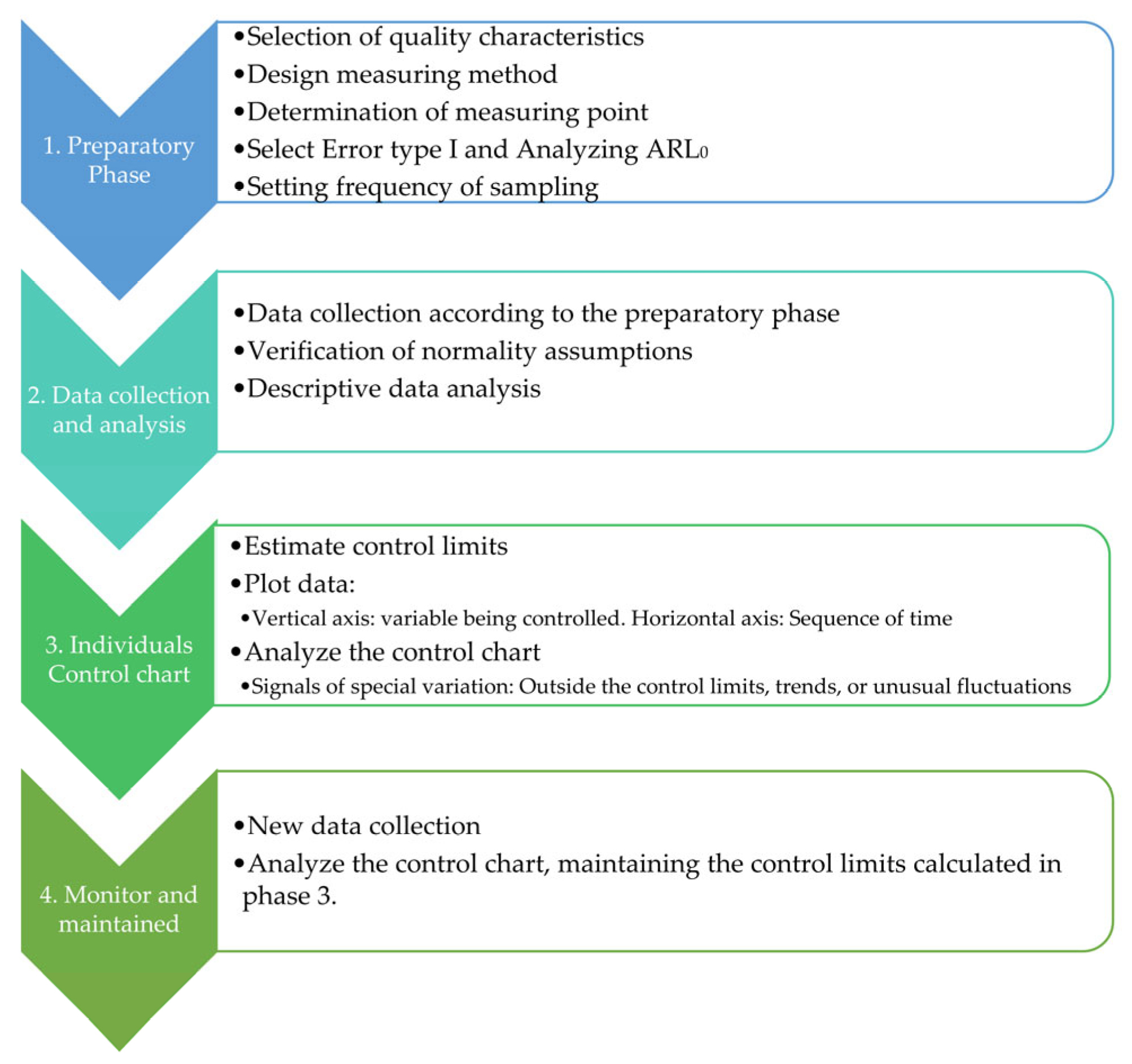
A control chart is a valuable statistical tool utilized for monitoring and analyzing process variation over time. Within control charts, the individual control chart, often referred to as an I-chart, stands out as a specific type that concentrates on tracking individual measurements or observations. Unlike other control charts that rely on aggregated or subgrouped data, the individual control chart operates on a sample size of one, enabling a more granular assessment of process performance. The analytical process involved in utilizing individual control charts is illustrated in Figure 1, providing a structured methodology for conducting the analysis.

The primary objective of an individual control chart is to distinguish between natural process variation and special causes of variation. It accomplishes this by establishing control limits based on the inherent variability of the process. The chart typically consists of a central line representing the process average and upper and lower control limits that indicate the acceptable range of variation. Individual data points are plotted over time, allowing for real-time monitoring of process performance and the detection of any deviations from the expected behavior.

By analyzing an individual control chart, one can glean valuable insights into the process under investigation. Deviations beyond the control limits or patterns such as trends, cycles, or unusual fluctuations can indicate the presence of special causes, which may require further investigation and corrective action. On the other hand, data points that fall within the control limits suggest that the process is operating within the expected range of variation and is considered statistically stable.

The process of conducting an analysis using individual control charts involves several steps. These typically include collecting individual measurements, calculating the process average and standard deviation, establishing control limits, plotting the data points on the chart, and interpreting the resulting patterns or trends. These steps ensure a systematic and rigorous approach to process monitoring and enable data-driven decision-making.

In conclusion, the individual control chart is a specific type of control chart that focuses on tracking individual measurements to monitor process variation. Its sample size of one allows for a more detailed assessment of process performance. By following the methodological process outlined in Figure 1, practitioners can effectively utilize individual control charts to identify special causes of variation and make informed decisions to improve and maintain process stability; in this case, the individual chart will be used for selecting degraded data. The calculation of control limits for an individual control chart involves determining the statistical boundaries that define acceptable process variation based on individual measurements or observations.

Therefore, let $x_i$ be a random variable representing individual observations of a process, and then the moving range (MR) of two successive observations to measure the process variability form as below:

$$M{R}_i=\left|x_{i+1}-x_i\right|, i=1, 2, \dots n-1$$

(1)

Hence, the control limits for the individual chart are usually specified as a multiple of the average of the moving ranges as [20]:

$$\begin{gathered} UCL: \overline{MR}+3\frac{\overline{MR}}{1.128} \\ LCL: \overline{MR}-3\frac{\overline{MR}}{1.128} \end{gathered}$$

(2)

where 1.128 is the constant used to adjust the position of the upper control limit in a control chart to ensure sensitivity to significant process deviations.

By monitoring the control chart, deviations beyond the control limits are represented as points that fall outside these limits. Such points indicate a greater variability than the natural process variability, which signifies an out-of-control condition.

3.2. Convolutional Neural Network

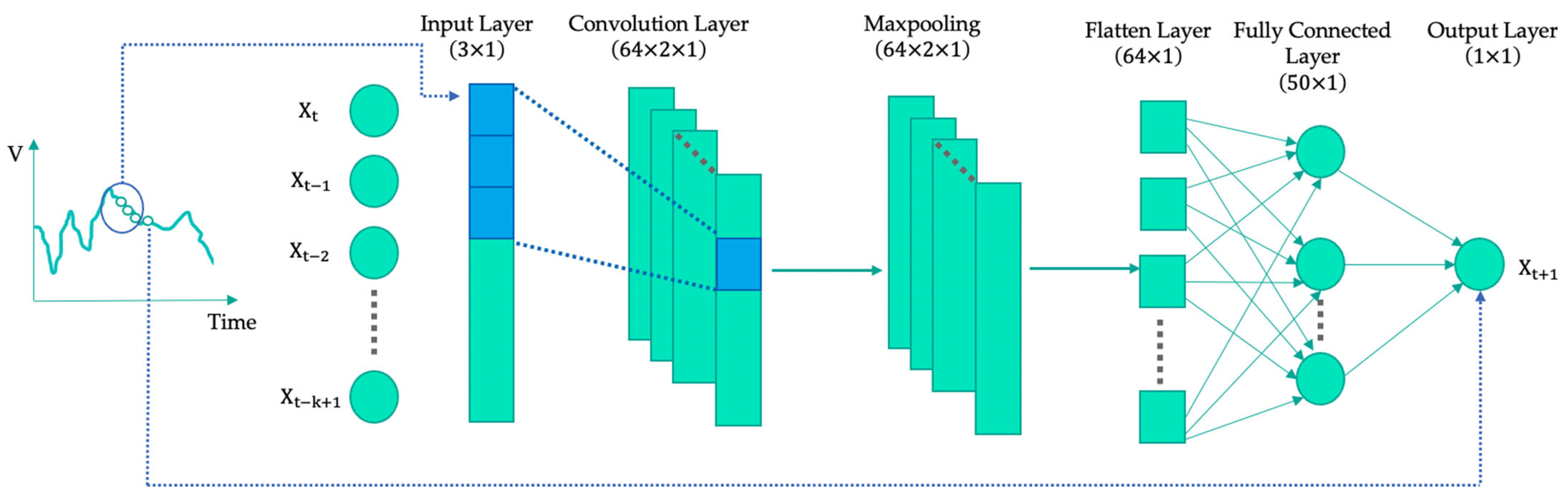
Convolutional neural networks (CNNs) are a type of artificial neural network (ANN) introduced by [21] in 1998. They are specifically designed for processing data with a known grid-like topology. Examples of such data include time-series data, which can be viewed as a 1D grid with regularly spaced time intervals, and image data, which can be seen as a 2D grid of pixels [22]. A typical CNN consists of various layers, including the input layer, convolutional layer, pooling layer, flatten layer, fully connected layer, and output layer. The input layer receives the input data and passes it to the convolutional layer. In this layer, filters are employed to extract targeted nonlinear patterns from the input data, resulting in feature maps. The pooling layer is used to down-sample these feature maps. Subsequently, the flatten layer transforms the multidimensional shape of the feature maps into a one-dimensional shape, which is then fed into the fully connected layer. The fully connected layer computes the final results based on these features [23,24,25]. Figure 2 provides an example of a CNN used for time-series prediction, where a univariate time series is used as input, and the output represents one prediction [26].

3.3. Long Short-Term Memory Neural Network

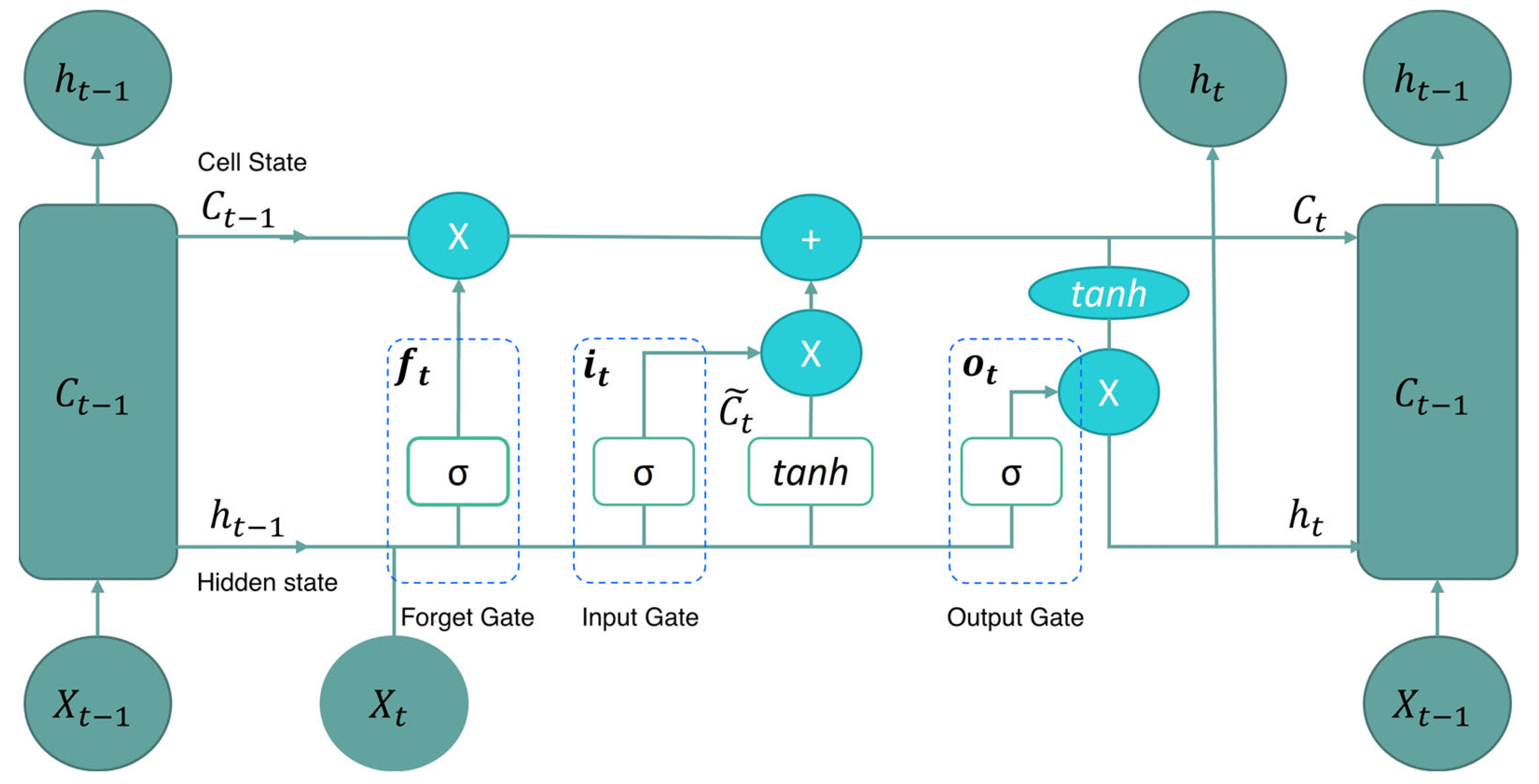
The long short-term memory (LSTM) neural network is a unique type of recurrent neural network (RNN) that excels at managing “long-term dependencies”. It was initially proposed by [27] in 1997. The LSTM network architecture comprises four neural networks and specialized memory blocks known as cells. By default, the LSTM network is designed to retain information over extended periods, and this information is stored within the cells. It is performed by three gates: the forget gate ${(f}_t)$, the input gate ${(i}_t)$, and the output gate $\left(o_t\right)$. These gates determine the significance of information and decide what should be retained or discarded. The LSTM cell consists of two primary states: the cell state ${(C}_{t-1}$) and the hidden state ${(h}_{t-1})$. These states are continuously updated and carry information from previous time steps to the current one. The cell state serves as the repository for long-term memory, and the hidden state acts as the repository for short-term memory. Figure 3 shows the structure of an LSTM network.

The forget gate serves the purpose of determining whether to retain or discard information. It evaluates both the current sequence and the prior state information to decide which data are irrelevant and should be discarded. A sigmoid activation is necessary in this context to constrain the information within a range between one and zero. The computation within the forget gate can be achieved by using [28]:

$$f_t=\sigma ({\mathit{W}}_f{\mathit{X}}_t+{\mathit{U}}_f{h}_{t-1}+{\mathit{b}}_f)$$

(3)

The forget gate can accept data from the prior hidden state $h_{t-1}$ and the sequence input ${\mathit{X}}_t$. Then, the data can be added with a bias ${(\mathit{b}}_f)$ and multiplied by the weights ${(\mathit{W}}_f, {\mathit{U}}_f)$. Next, the values are followed through the sigmoid activation $(\sigma$) to be kept in the cell state or removed.

The input gate gathers information from $h_{t-1}$ and ${\mathit{X}}_t$ to update information in the cell state. The data undergoes two functions: sigmoid and tanh. Sigmoid activation is employed to determine important information that needs updating. The values of ${\mathit{X}}_t$ and $h_{t-1}$ are added with a bias ${(\mathit{b}}_i)$ and then multiplied by a weight ${(\mathit{W}}_i, {\mathit{U}}_i)$ to generate a vector ranging between zero and one. The sigmoid value is utilized to assess crucial data using the following equation [28]:

$$i_t=\sigma ({\mathit{W}}_i{\mathit{X}}_t+{\mathit{U}}_i{h}_{t-1}+{\mathit{b}}_i)$$

(4)

Then, Equation (4) can be used to obtain the tanh function used to convert the data between −1 and 1 using the following equation. This was to create a new vector that needed to be applied to the cell.

$${\tilde{C}}_t=tanh\left({\mathit{W}}_c{\mathit{X}}_t+{\mathit{U}}_c{h}_{t-1}+{\mathit{b}}_c\right),$$

(5)

where ${\mathit{W}}_c$ and ${\mathit{U}}_c$ are the weights and ${\mathit{b}}_c$ is the bias.

The process is completed through the inclusion of two steps within the output gate. The initial step involves acquiring the current input ${\mathit{X}}_t$ and the previous hidden state $h_{t-1}$. These values are then fed into the sigmoid function. Similar to the other two gates, sigmoid activation is applied here, where they are multiplied by the weights ${(\mathit{W}}_o, {\mathit{U}}_o)$ before being summed with a bias ${(\mathit{b}}_o)$ [28].

$$o_t=\sigma \left({\mathit{W}}_o{\mathit{X}}_t+{\mathit{U}}_o{h}_{t-1}+{\mathit{b}}_o\right)$$

(6)

The next step involves acquiring the value of the cell state and passing it through the tanh activation. Subsequently, the product of the tanh function’s value and the output of the sigmoid is used to ascertain the information for the hidden state.

$$h_t=o_{t }\ast tanh\left(C_t\right)$$

(7)

4. ICC-CNN-LSTM Methodology

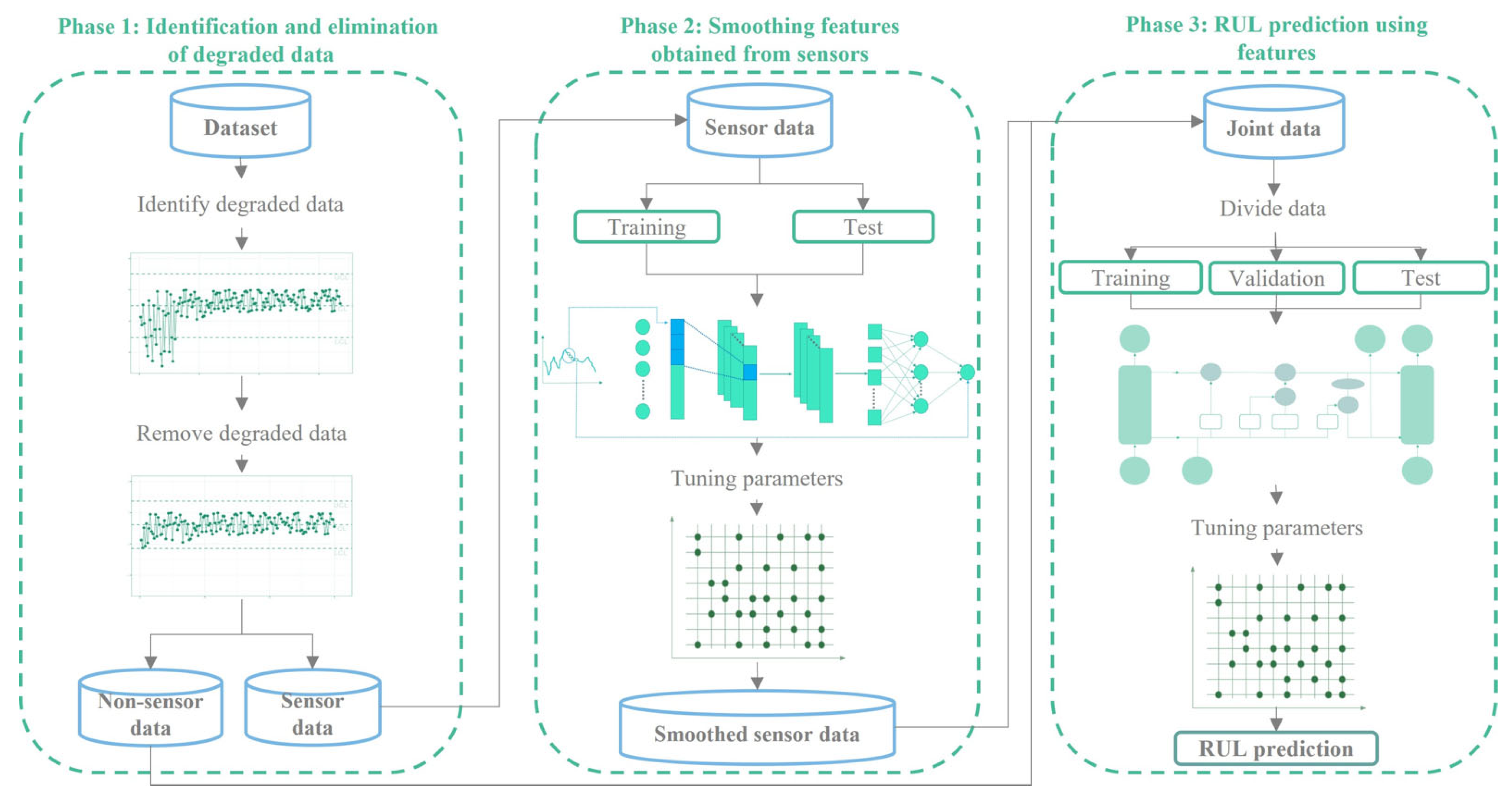
In this study, we introduce the ICC-CNN-LSTM approach for predicting the RUL from based on battery-related features. Our methodology encompasses three key phases: (1) identification and elimination of degraded data, (2) smoothing features obtained from sensors, and (3) RUL predicting using features. Figure 4 provides a visual representation of the proposed methodology.

Phase 1: Identification and elimination of degraded data. In this phase, degraded data are detected using an individual control chart. The degraded data are those points that fall outside the limits LCL and UCL. Once these data are identified, they are removed from the database. The features of this resulting database are divided into two groups: those obtained from sensors and those not obtained from sensors.

Phase 2: Smoothing features obtained from sensors. Each feature is smoothed through a CNN. The proposed architecture consists of three layers. The first convolutional layer uses RELU as an activation function and contains F filters of size two. The second pooling layer has two pool sizes and uses an operation max pooling [29,30]. The third flatten layer is connected through two dense layers [13]. The first dense layer has N neurons and the second one has one neuron. In the training phase, we used an Adam model optimization algorithm [11,31] with an initial learning rate of L. Also, we used E epochs [6,11,32]. The hyperparameters F, N, L, and E are optimizers. Non-sensor features are not smoothed; they are left in their natural state.

Phase 3: RUL prediction using features. The predicted value of the RUL is obtained by the LSTM network. The architecture proposed consists of two LSTM layers, that capture the short-run and long-run dependencies on the predictive value [11,13]. We used N1 and N2 neurons in the first and second LSTM layer. Also, in the first LSTM layer, we used tanh as an activation function and a return sequence. Between each of the LSTM layers, we used two dropout layers with dropout rates of D1 and D2 as a regularization method to control the overfitting [6,29,33]. Finally, after the second dropout layer, we added a dense layer with one neuron. In the training phase, we used an Adam model optimization algorithm with an initial learning rate of L and we used E epochs. The hyperparameters N1, N2, D1, D2, L, and E are optimizers found using recommended values from other studies and empirical tests in an effort to find the most appropriate configuration.

The features and the observed RUL are divided into three sets: train, validation, and test. Train data enter the LSTM network with the proposed architecture. The validation data are then fed into the trained network to optimize the network hyperparameters: neuron number, dropout rate, learning rate, and epochs. Finally, the test data enter the new optimized network to calculate performance measures.

5. Results

In this section, we outline the implementation of the proposed methodology using the NASA dataset. Section 5.1 provides a brief overview of the data, followed by Section 5.2 with a statistical description of the features utilized for RUL prediction. Subsequently, in Section 5.3, we detail the methodology implementation, including the identification of degraded data, feature smoothing, and RUL prediction. Section 5.4 provides a comparison of RUL estimation models. Finally, in Section 5.5, an analysis of the prediction accuracy is presented, considering various scenarios. This comprehensive examination provides valuable insights into the performance and effectiveness of the implemented methodology for the NASA dataset.

5.1. Data

To implement the methodology outlined in Section 3, we used a dataset consisting of four batteries obtained from the National Aeronautics and Space Administration (NASA), referred to as B5, B6, B7, and B18. These batteries have been extensively employed in RUL prediction studies [34]. The experimental trials with the batteries were conducted at an ambient temperature of 24 °C and involved three distinct operating profiles: charge, discharge, and impedance.

For batteries B5, B6, and B7, a comprehensive analysis was conducted on 168 charge and discharge cycles, resulting in a total of 50,285 records available for each of these batteries. As for battery B18, 132 charge and discharge cycles were examined, providing a total of 34,866 records for analysis. The features employed for predicting the RUL included voltage (V), current (A), temperature (°C), and SOH (%).

All analyses were conducted using the R programming language [35] within the integrated programming environment (IDE) of RStudio [36]. The qcc library [37] was used to identify degraded data through individual control charts, and the cnnlstm R pakage was employed for noise smoothing of sensor data and RUL prediction using CNN and LSTM networks, respectively. These libraries facilitated efficient implementation of the proposed methodologies, enabling accurate data analysis and prediction tasks.

The current version of the cnnlstm R package is hosted on GitHub. You can explore the GitHub repository by visiting https://github.com/cjrincon/cnnlstm (accessed on 23 September 2023). To use the cnnlstm R package we suggest employing Google Colab, an interactive notebook provided by Google, that allows for writing and executing R and Python code. To use the notebook with an R kernel, please access the following URL: https://colab.research.google.com/drive/1H3eyFSEGSkis1IceLmte7ZAw9sCaHt5I?usp=sharing (accessed on 23 September 2023).

5.2. Descriptive Analysis

Table 1. Descriptive measures of the features measured in each battery.

Features	Battery	Median	Mean	Standard Deviation
Capacity	5	1.54	1.56	0.18
	6	1.47	1.53	0.23
	7	1.61	1.63	0.15
	18	1.61	1.58	0.16
Voltage	5	3.51	3.52	0.23
	6	3.47	3.46	0.25
	7	3.52	3.52	0.27
	18	3.50	3.50	0.25
Current	5	−2.01	−1.81	0.61
	6	−2.01	−1.77	0.65
	7	−1.99	−1.91	0.39
	18	−2.01	−1.84	0.55
Temperature	5	32.83	32.82	3.99
	6	32.94	32.84	4.14
	7	32.29	32.37	4.00
	18	31.12	31.08	3.65
Time	5	1537	1546	906.64
	6	1537	1546	906.64
	7	1537	1546	906.64
	18	1537	1547	908.37
SOH	5	82.9%	84.1%	10%
	6	72.4%	74.9%	11%
	7	84.9%	86.4%	8%
	18	86.6%	85.4%	8%

presents descriptive measures of the features used in the RUL prediction, categorized for each of the four analyzed batteries. These measures offer insights into the characteristics of the features, helping to understand their overall patterns and variability. These measures include the mean, which provides the average value, and the median, which represents the middle value. Examining these central tendency measures allows us to grasp the typical values exhibited by the features and understand their general levels or positions within the dataset.

In addition to central tendency, measures of dispersion provide essential information about the spread or variability of the features. These measures include the standard deviation, which quantifies the average amount of deviation from the mean. By analyzing this measure, we can identify the degree of variability within each. This understanding is crucial for detecting any potential outliers or anomalies that may significantly impact the RUL prediction process. The expression of SOH and RUL for a critical component of an EV in terms of capacity is shown in [4,9,10].

Table 1 reveals that time exhibits the highest variability among the four batteries, indicating significant variations in its values. On the other hand, SOH displays the least variability among the considered features. This suggests a relatively consistent and stable pattern in SOH values across the batteries. Furthermore, it can be observed that the time feature contributes to 69% of the overall variability, followed by temperature with 17%. In contrast, the remaining features contribute less than 3% each. Hence, it can be concluded that the features of SOH, current, voltage, and capacity exhibit significant stability in their values across the analyzed five batteries. Understanding the varying degrees of variability among these features is crucial in assessing their potential impact on the prediction and formulating appropriate strategies to account for their influence.

5.3. Implementation of the Methodology

To identify degraded data, we employed an individual control chart, where the control limits and centerline were calculated using the qcc function from the qcc package, available in https://cran.r-project.org/web/packages/qcc/index.html (accessed on 23 September 2023). The control charts were plotted using the ggplot2 package, available in https://cran.r-project.org/web/packages/ggplot2/index.html (accessed on 23 September 2023).

For smoothing the sensor-measured features, we used the architecture of the proposed CNN outlined in Section 2 of the methodology. To optimize the hyperparameters, we used the hyperparameter optimization function from the cnnlstm R package. The function resulted in the use of 64 filters in the convolutional layer, 100 neurons in the first dense layer, a learning rate of 0.001 in the Adam algorithm, and training for 500 epochs.

For the RUL prediction, we used the proposed architecture of the LSTM neural network from Section 2 of Methodology. The hyperparameter optimization process for the neural network resulted in 128 neurons in the first LSTM layer, a dropout rate of 0.3 in the first layer, 32 neurons in the second LSTM layer, and a dropout layer with a rate of 0.2. Furthermore, the optimization function defined a learning rate of 0.01 with 500 epochs for training the predictive model.

The performance of CNN and LSTM networks was evaluated based on: mean square error (MSE), root mean square error (RMSE), mean absolute percentage error (MAPE), and mean absolute error (MAE). A smaller value of these metrics indicates a better RUL prediction (see Supplementary Material for further details).

5.3.1. Identification and Elimination of Degraded Data

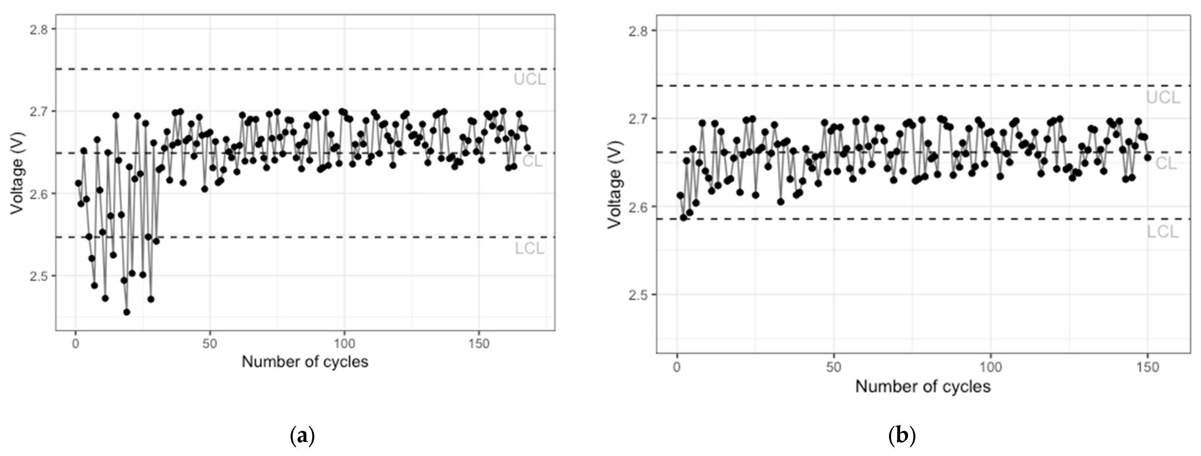
Figure 5a illustrates the individual control chart representing all voltage records for battery 5, providing a comprehensive overview of its performance. In contrast, Figure 5b presents the individual control chart specifically for the voltage records of battery 5 that were not considered degraded data. Similar individual control charts were constructed for batteries 6, 7, and 18 to assess their respective voltage behaviors.

Comparing the control limits between the two charts reveals a significant observation: the identification and elimination of degraded data lead to a noticeable reduction in voltage measurement variability. Figure 5a demonstrates the presence of 15 cycles that were identified as degraded and subsequently removed. The resulting chart, Figure 5b, showcases the improved condition after the elimination of those cycles.

By visualizing the data on these individual control charts, we gain valuable insights into the effects of removing degraded data on voltage variation. The control limits provide a reference range within which the voltage measurements are expected to fall. The narrower control limits in Figure 5b indicate that after eliminating the degraded cycles, the voltage measurements for battery 5 exhibit reduced variability and increased stability. Similarly, the same trend was observed in batteries 6, 7, and 18.

5.3.2. Smoothing of Features Obtained from Sensors

Table 2. Performance metrics of the features measured in each battery.

Feature	Battery	MSE	RMSE	MAE	MAPE
Current	5	0.0001	0.0115	0.0068	0.86
	6	0.0001	0.0112	0.0071	0.95
	7	0.0002	0.0131	0.0065	0.94
	18	0.0001	0.0071	0.0053	0.63
Temperature	5	0.0003	0.0181	0.0117	4.90
	6	0.0002	0.0152	0.0096	4.63
	7	0.0003	0.0169	0.0109	4.24
	18	0.0003	0.0162	0.0107	4.01
Voltage	5	0.0002	0.0145	0.0086	1.32
	6	0.0005	0.0223	0.0105	1.54
	7	0.0006	0.0249	0.0133	1.98
	18	0.0007	0.0261	0.0149	2.56

displays the performance metrics for smoothing the features of current, temperature, and voltage for each of the four analyzed batteries. The current feature exhibited the lowest performance metric values, particularly in battery 18. Overall, all features showcased small performance metric values. It can be observed that when the sensor-captured features (temperature, current, and voltage) are subjected to smoothing, battery 5 demonstrates the most favorable behavior. Moreover, it is noteworthy that the current feature achieves the highest performance during the smoothing phase.

The measure that exhibits the highest discriminatory power when analyzing the deviation per battery is the MSE for battery 5. Additionally, for batteries 7 and 18, the MAPE demonstrates significant discriminatory power. In the case of battery 6, the RMSE stands out as the measure with the highest discriminatory power. These findings reaffirm the importance of utilizing different performance measures to analyze models of this nature, as they provide valuable insights into specific aspects of each battery’s performance. Additionally, both current and temperature consistently exhibit lower variability in the performance measures across all analyzed batteries. This indicates that the smoothing process achieves greater stability for these two features. The reduced variability suggests that the smoothing technique effectively mitigates the fluctuations and noise present in the data, resulting in more stable and reliable performance measures for current and temperature across the batteries.

5.3.3. RUL Prediction Using Features

Based on the results shown in

Table 3. Performance metrics under the split data.

Split	MSE	RMSE	MAE	MAPE
Train	0.0002	0.0123	0.0101	4.80
Validation	0.0003	0.0165	0.0130	6.28
Test	0.0003	0.0174	0.0142	8.66

, it can be concluded that performance values for the training, validation, and test sets are relatively low, indicating that the model performs well in terms of minimizing the performance metrics. When examining the performance of the validation and test sets, it is evident that the validation set exhibits better performance. Across all the metrics, the differences between the training and validation sets are relatively small. The slight increases in performance measures between the training and validation sets suggest comparable or slightly lower performance in the validation set. However, when comparing the training set to the test set, more significant percentage differences indicate a decline in performance in unseen data. The observed results indicate that the model’s performance in the validation set is on par with or slightly inferior to its performance in the training set. This suggests that the model’s predictions generally align closely with the actual values, although there is a slight increase in MSE in the validation and test sets. Additionally, RMSE, MAE, and MAPE further validate the model’s capability to make accurate predictions. These performance metrics demonstrate that the model’s predictions exhibit a relatively low percentage difference when compared to the actual values.

5.4. Comparison of RUL Estimation Models

We compared the accuracy of our proposed ICC-CNN-LSTM methodology in different scenarios with LSTM, ICC-LSTM and CNN-LSTM. Additionally, we compared our model with models reported in the literature for the database and batteries under study. To evaluate accuracy, we used RMSE, which is the most commonly reported performance metric in published studies. The results of the models are shown in

Table 4. RSME for RUL estimation per model.

Author	Model	Battery 5	Battery 6	Battery 7	Battery 18
Proposed model	LSTM	0.0983	0.0430	0.0878	0.1100
	CNN-LSTM	0.0174	0.0257	0.0157	0.0190
	ICC-LSTM	0.0878	0.0379	0.0835	0.0930
	ICC-CNN-LSTM	0.0166	0.0118	0.0125	0.0143
[8]	RNN	0.1051	0.1131	0.1132	0.0551
	LSTM	0.0135	0.1216	0.0284	0.0498
	RVM	0.0783	0.0784	0.1138	0.0601
	HA-FOSELM	0.0980	0.0434	0.1021	0.0274
[11]	MC-RNN	0.0255	0.0488	0.0284	0.0645
	MC-GRU	0.0282	0.0375	0.0269	0.0568
	MC-SRU	0.0322	0.0624	0.0296	0.0800
	MC-LSTM	0.0208	0.0428	0.0231	0.0449
[19]	LSTM	0.1130	0.1216	-	0.0498
	RNN	0.1047	0.1131	-	0.0551
	RVM	0.0784	0.0784	-	0.0601
	PA-LSTM	0.0937	0.0499	-	0.0324

.

Table 4 shows that for batteries 6, 7 and 18, the proposed model presents the best performance compared to the other models. In the case of battery 5, the model for LSTM network has an RSME of 0.0135, whereas the proposed model has an RSME of 0.0166; we can observe that RUL estimation for battery 5 in the proposed model has a performance that is nearly the same in terms of accuracy. The cumulative performance of the proposed model exceeds that of other models reported in the literature by at least a factor of two.

In addition, it is observed that in the CNN-LSTM scenario, there is an improvement in the prediction of the RUL compared to the literature review scenarios. This highlights the innovativeness of our proposed ICC-CNN-LSTM. In the same way, the elimination of the degraded data through ICC shows an improvement in the RMSE obtained in comparison with the other scenarios and models compared in the literature review.

5.5. Performance Comparation of Four Scenarios

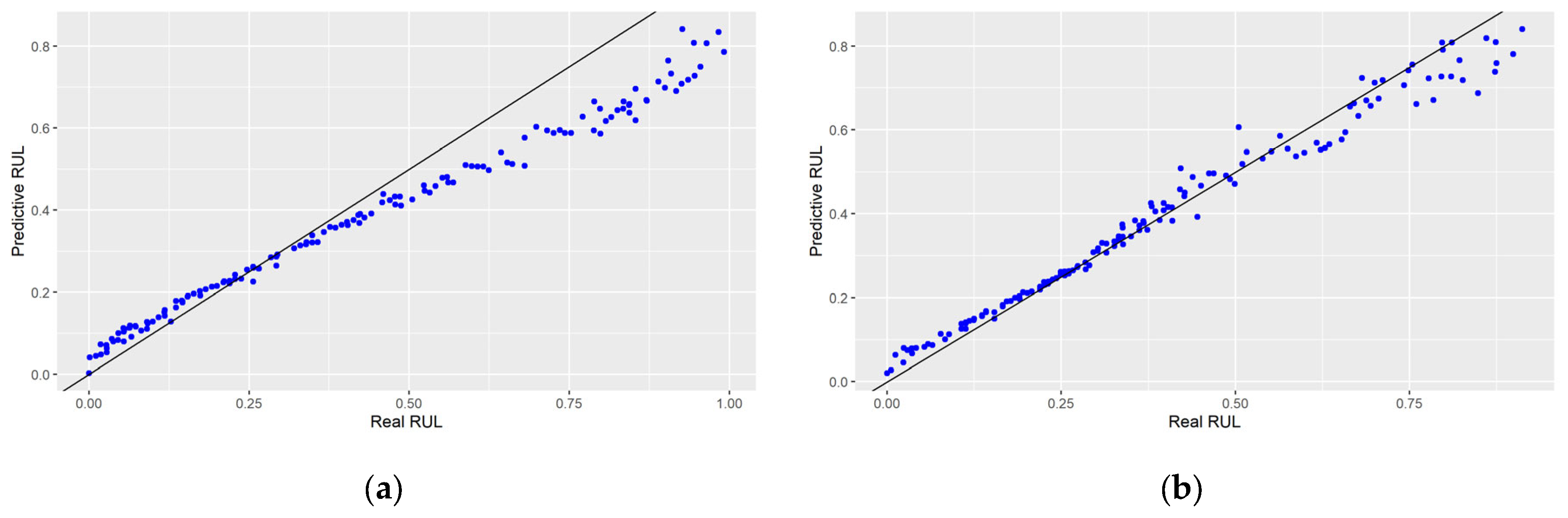
This section focuses on evaluating the RUL predictions based on the implementation of the phases outlined in the proposed methodology: identification of degraded data, smoothing of sensor-derived features, and RUL prediction using features. In scenario 1, the RUL is predicted solely using the LSTM network, without considering the identification of degraded data or smoothing the noise from the sensor measurements. In scenario 2, the RUL is predicted using the hybrid CNN-LSTM model, with the noise in the sensor measurements being eliminated. On the other hand, in scenario 3, degraded data are identified, and the RUL is predicted using the LSTM network, without smoothing the noise from the sensor measurements. Finally, in scenario 4, the proposed methodology in this study is employed, encompassing the identification of degraded data, smoothing the noise from sensor measurements, and predicting the RUL using the LSTM network. Furthermore, the accuracy of the predictions is assessed using different split data: train, validation, test, and degradation.

Table 5. Scenarios to evaluate the accuracy of the RUL prediction.

Scenario	Split Data	Smoothing	Predictive Model
1	Train, validation, test	No	LSTM
2	Train, validation, test	Yes	CNN-LSTM
3	Train, validation, test, degradation	No	ICC-LSTM
4	Train, validation, test, degradation	Yes	ICC-CNN-LSTM

illustrates the four scenarios considered for evaluating the accuracy of the RUL predictions.

It is worth highlighting that the fourth scenario corresponds to the proposed approach in this study, and to generate it, the methodology described earlier is applied using the cnnlstm R package. Furthermore, it should be emphasized that the fourth scenario represents the implementation of the proposed methodology outlined in this paper, utilizing the cnnlstm R package.

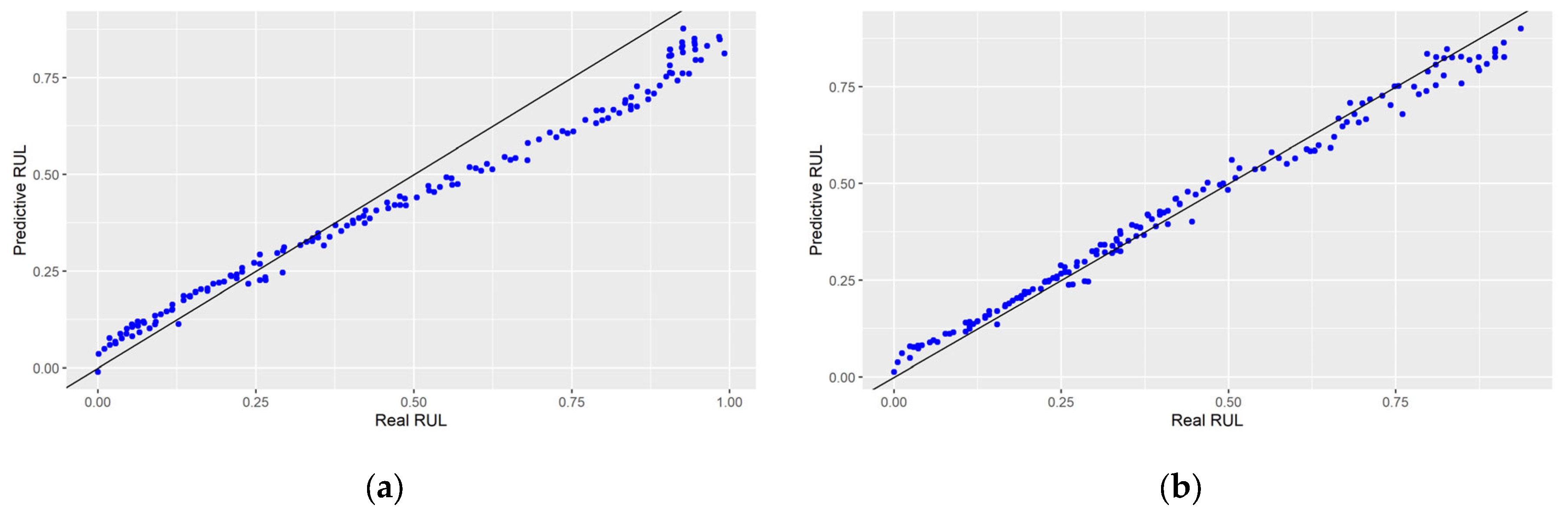
Figure 6, Figure 7, Figure 8 and Figure 9 display scatterplots showing the relationship between the real values and predicted values of the RUL. Each figure presents the scatterplots for batteries, 5, 6, 7 and 18. Figure 6 presents the predictive model from Scenario 1, where the LSTM network was implemented. It is evident that battery 6 exhibits a strong alignment between the predicted values and the true values. However, for batteries 5 and 7, several predictions appear to be underestimated in comparison to the real values, as indicated by the points lying below the line. Moreover, in the case of battery 18, the predictive model demonstrates poor alignment with the real values, suggesting an overfitting issue where the predictions excessively conform to the real battery capacity values.

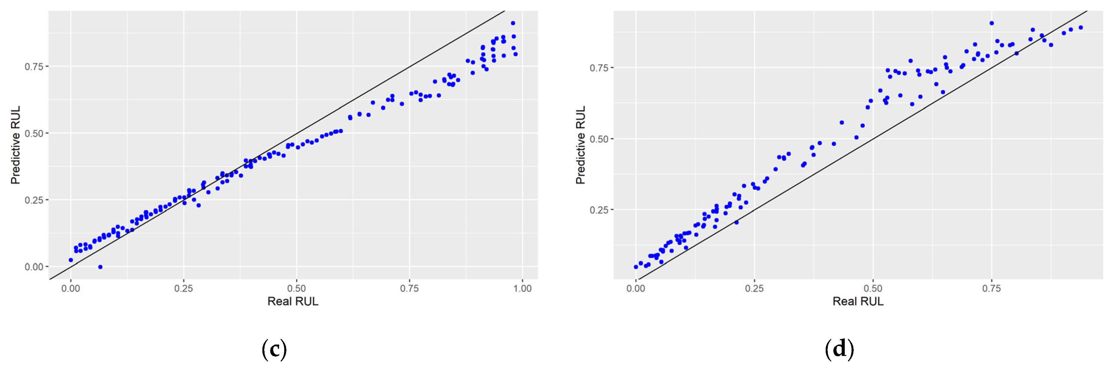
Figure 7 displays the results obtained from Scenario 2, which involves three datasets: training, validation, and testing. In this scenario, a combination of a CNN-based smoothing model and an LSTM predictive model is implemented. Overall, a good fit of the prediction is observed when compared to the real capacity values of each battery. This scenario incorporates the data smoothing process performed using sensors, highlighting the significance of the smoothing model in generating accurate predictions with the LSTM model. However, a slight overfitting is observed in the predictions for batteries 6 and 18, as several data points are situated above the reference line, indicating a deviation from the real values. These findings emphasize the importance of striking a balance between data smoothing and accurate prediction to ensure reliable results. Further optimization of the model’s parameters and fine-tuning may be required to address the overfitting issue and enhance the overall accuracy of the predictions for batteries 6 and 18.

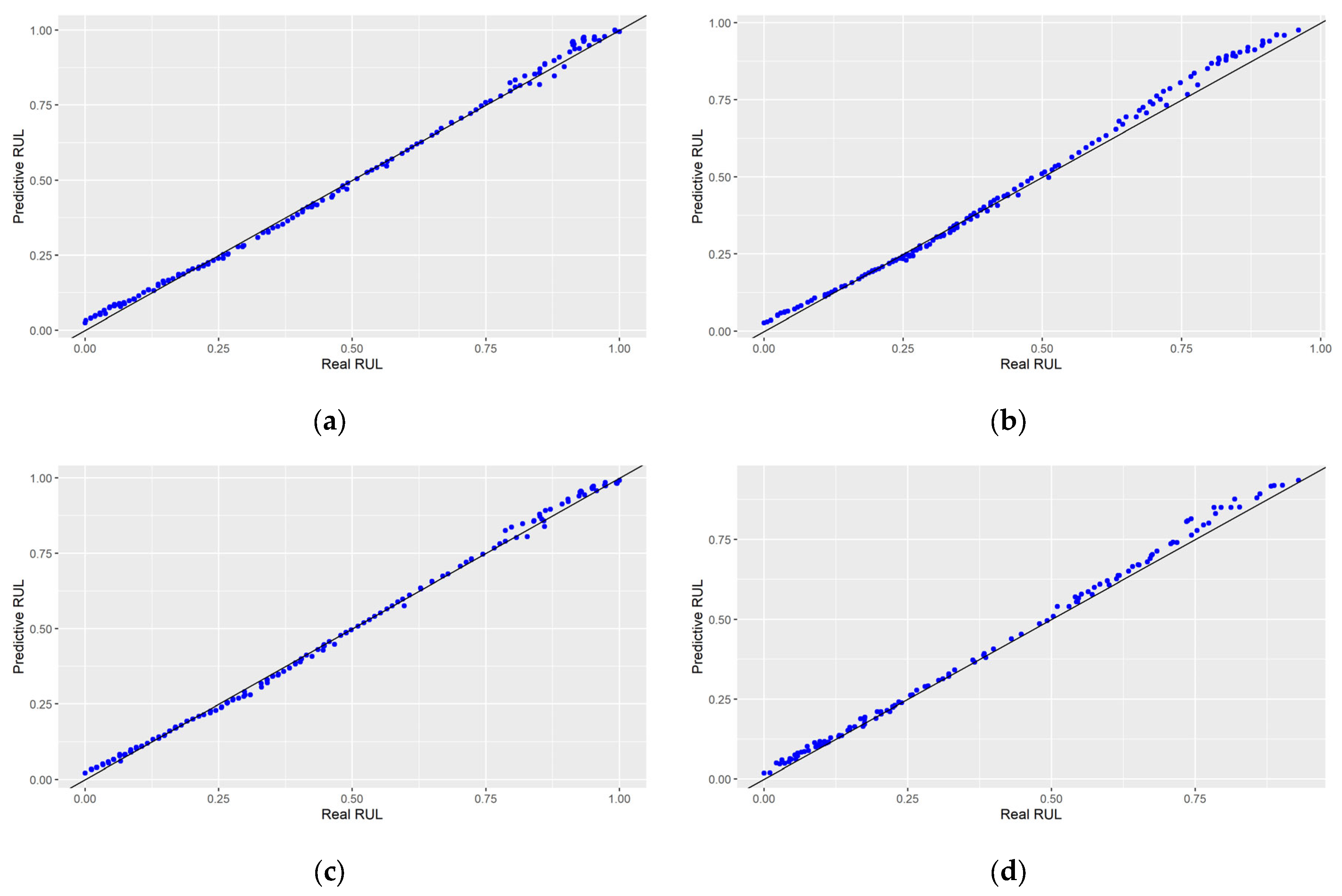
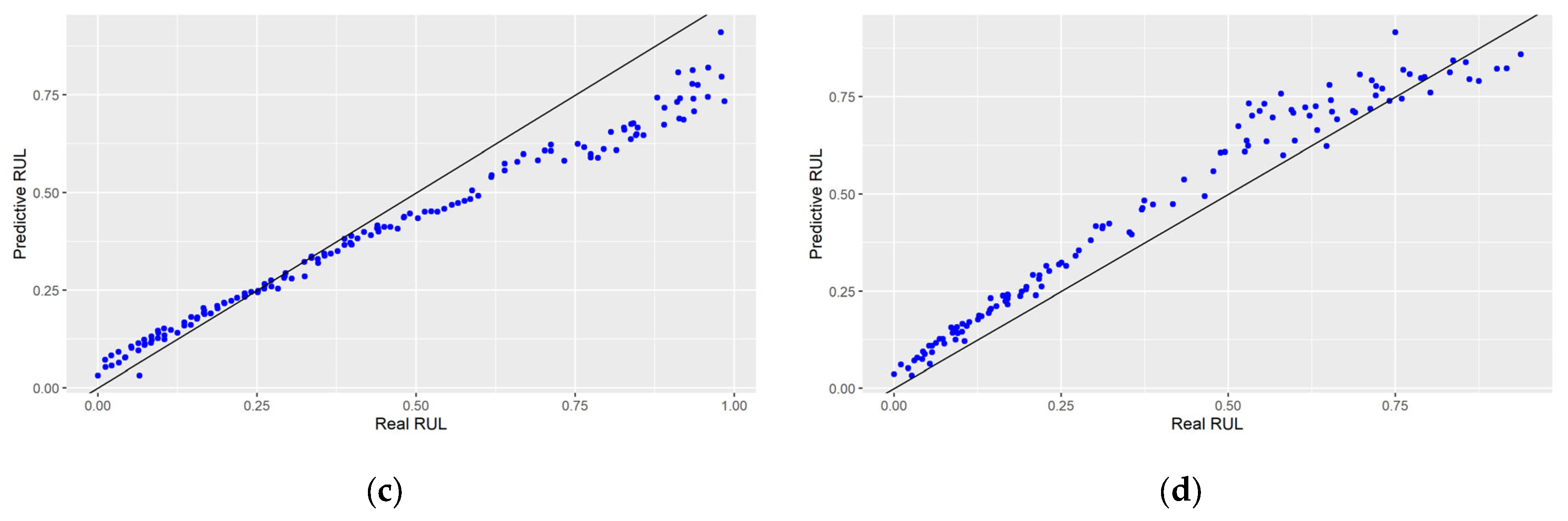
Figure 8 presents the results obtained from the implementation of four datasets: training, validation, testing, and degradation from Scenario 3. In this case, only the predictive model with the ICC-LSTM network is utilized to make the predictions. Overall, a poor fit of the predictions is observed for each of the batteries. Battery 5 exhibits initial overfitting in the predictions, followed by an underestimation towards the end, resulting in a poor overall fit. For battery 6, there is a consistent overfitting pattern in the predictions, with the majority of data points remaining above the line. Battery 7 shows similar behavior to battery 5, with an initial overfitting and subsequent underestimation, leading to inaccuracies in the model’s precision. When evaluating battery 18, less alignment is observed in the predictive model, as there is greater variability in the data points compared to the expected line. This indicates that the model is not capable of accurately capturing the capacity behavior in this battery. These findings highlight the limitations of the predictive model using the ICC-LSTM network in Scenario 3. The identified overfitting, underestimation, and lack of precision in capturing the capacity behavior indicate the need for further refinement and improvement of the model. Additional analysis and adjustments may be necessary to enhance the predictive capabilities for each battery to achieve more accurate and reliable results. Additionally, the results obtained from Scenario 3 indicate that relying solely on the predictive model with the ICC-LSTM network does not yield satisfactory predictions for the analyzed batteries. The observed overfitting, underestimation, and lack of precision demonstrate the challenges in accurately capturing the capacity behavior using this approach.

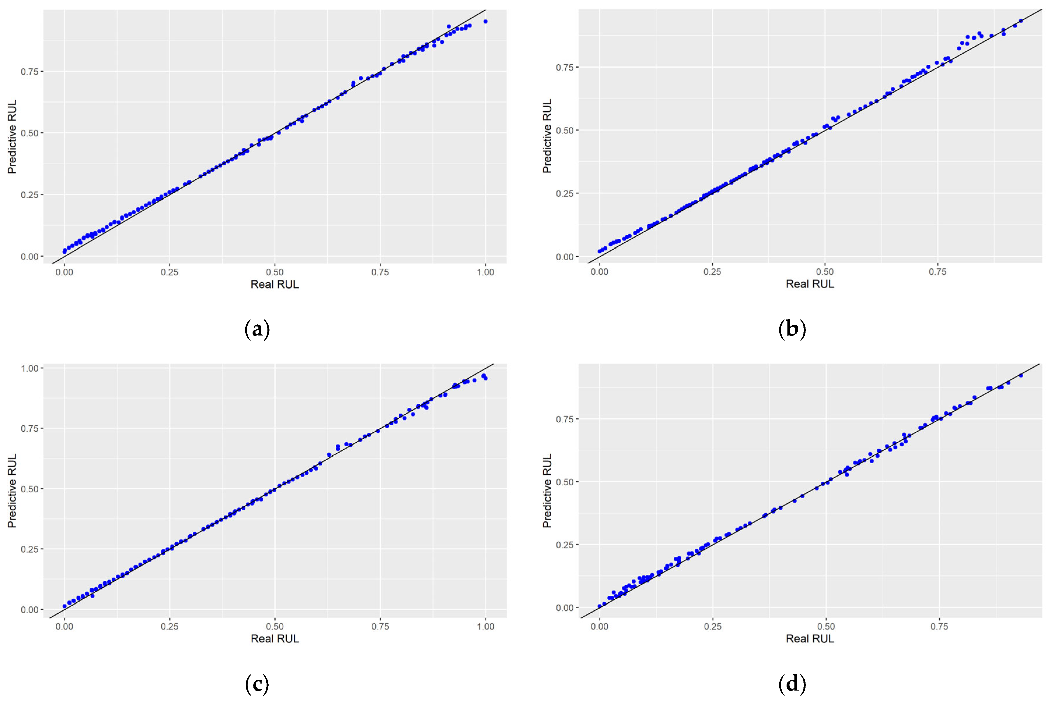
Figure 9 illustrates the results obtained from evaluating the fourth scenario, which involves dividing the data into four sets: training, validation, testing, and degradation. In this case, both the CNN-based smoothing model and the LSTM-based predictive model are implemented. The results obtained from evaluating the fourth scenario demonstrate the effectiveness of the combined approach involving data division, CNN-based smoothing, and LSTM-based predictive modeling in accurately predicting battery capacity. By dividing the data into distinct sets and incorporating both data smoothing and predictive models, a strong alignment between predicted and real capacity values is achieved. This scenario highlights the importance of considering various aspects of capacity modeling and prediction, particularly throughout charge and discharge cycles. The use of data smoothing techniques obtained from sensors significantly contributes to improving the accuracy of capacity predictions. Additionally, the identification of degradation data plays a vital role in enhancing the model’s fit. The observed alignment between predicted and real values, closely following the expected trend, further validates the reliability and precision of the proposed approach. These findings emphasize the value of integrating data division, data smoothing, and predictive modeling for accurate capacity predictions in engineering applications.

Table 6. Performance metrics of the four batteries under each of the analyzed scenarios.

Scenario	Battery	MSE	RMSE	MAE	MAPE
1	5	0.0097	0.0983	0.0841	25.0
	6	0.0019	0.0430	0.0377	15.1
	7	0.0077	0.0878	0.0729	21.6
	18	0.0121	0.1100	0.1030	31.5
2	5	0.0003	0.0174	0.0142	8.66
	6	0.0007	0.0257	0.0189	6.40
	7	0.0003	0.0157	0.0127	5.28
	18	0.0004	0.0190	0.0140	7.67
3	5	0.0077	0.0878	0.0688	21.8
	6	0.0014	0.0379	0.0292	11.7
	7	0.0070	0.0835	0.0621	18.3
	18	0.0087	0.0930	0.0797	24.6
4	5	0.0003	0.0166	0.0135	8.54
	6	0.0001	0.0118	0.0089	5.71
	7	0.0002	0.0125	0.0090	5.19
	18	0.0002	0.0143	0.0117	7.11

presents the four performance metrics considered for each scenario and different batteries. The values in bold represent the minimums for each metric. Among the four scenarios, scenario 4 consistently exhibits the best performance measures across all batteries. Specifically, battery 6, under scenario 4, demonstrated the best metrics, indicating a more accurate prediction of RUL behavior. It is observed that the proposed methodology represents an improvement compared to other scenarios. Likewise, in scenarios where a hybrid model with data smoothing is proposed, better performance is achieved in the results, as seen in the metrics obtained in scenarios 2 and 4. This is followed by scenario 3, where the removal of degradation data is considered to generate a higher-quality dataset for the predictive model.

6. Conclusions

Considering features beyond capacity when predicting RUL is critical to building a more robust methodology. This approach significantly improves prediction accuracy by capturing a wider range of influencing factors. The limitations of a prediction model with a single feature versus a prediction model with multiple features are significant in various engineering contexts. Prediction models with a single feature often lack accuracy due to their inability to account for complex relationships and dependencies, resulting in reduced predictive accuracy and limited generalizability, making them susceptible to noise and instability. Therefore, the proposed methodology is considered to capture critical interactions and context, avoiding biases and reducing assumptions. In addition, it was verified that the proposed methodology is adequate to detect real anomalies.

The use of ICC plays a key role in increasing the robustness and reliability of the analytical process. These charts serve to effectively filter out cycles that deviate from the expected random behavior attributed to the same underlying condition. In doing so, they act as a rigorous quality control mechanism, ensuring the integrity of the dataset used to build the predictive model. Having an objective technique for removing from the database those cycles that are degraded ensures that the resulting model accurately reflects the natural variability inherent in the process under study, a critical aspect of achieving accurate predictions and informed decisions. Consequently, incorporating this technique into the methodology showed that the performance of the model is improved compared to other models developed.

Throughout the data collection process, raw sensor data often contains noise caused by external environmental interference. In such instances, employing CNN networks can effectively reduce this noise and significantly enhance the accuracy of RUL predictions. By implementing this proposed methodology, a notable improvement in RUL prediction accuracy was achieved, which proves to be of immense significance for battery health analysis and assessment. Simultaneously, the integration of an LSTM network enables effective learning of long-term dependencies among the time units of the provided data. This combination of methods enables a comprehensive and accurate prediction process, considering both feature precision and long-term data relationships.

The R package cnnlstm is an open-source implementation of the ICC-CNN-LSTM methodology that allows users to predict RUL. This package includes functions for data splitting, generating CNN models to smooth data obtained from sensors, creating LSTM models to predict variables with nonlinear behavior over time, and evaluating the performance of prediction models. The created functions are generic and can be used in any field of knowledge that involves similar patterns to RUL prediction.