Estimation of 3D Permeability from Pore Network Models Constructed Using 2D Thin-Section Images in Sandstone Reservoirs

Abstract

Using thin-section images to estimate core permeability is an economical and less time-consuming method for reservoir evaluation, which is a goal that many petroleum developers aspire to achieve. Although three-dimensional (3D) pore volumes have been successfully applied to train permeability models, it is very expensive to carry out. In this regard, deriving permeability from two-dimensional (2D) images presents a novel approach in which data are fitted directly on the basis of pore-throat characteristics extracted from more cost-effective thin sections. This work proposes a Fluid–MLP workflow for estimating 3D permeability models. We employed DIA technology combined with artificial lithology and pore classification to calculate up to 110 characteristic parameters of the pore-throat structure on the basis of 2D rock cast thin sections. The MLP network was adopted to train the permeability prediction model, utilizing these 110 parameters as input. However, the accuracy of the conventional MLP network only reached 90%. We propose data preprocessing using fluid flow simulations to improve the training accuracy of the MLP network. The fluid flow simulations involve generating a pore network model based on the 2D pore size distribution, followed by employing the lattice Boltzmann method to estimate permeability. Subsequently, six key structural parameters, including permeability calculated by LBM, pore type, lithology, two-dimensional porosity, average pore–throat ratio, and average throat diameter, were fed into the MLP network for training to form a new Fluid–MLP workflow. Comparing the results predicted using this new Fluid–MLP workflow with those of the original MLP network, we found that the Fluid–MLP network exhibited superior predictive performance.

1. Introduction

Permeability, which serves as a key parameter reflecting the physical characteristics of oil and gas reservoirs and plays a crucial role in evaluating reservoir quality and predicting oil and gas production [1], is a fundamental property of rock that determines its ability to allow fluid to flow under specific pressure differentials. However, accurately estimating permeability at various scales during reservoir evaluation has long posed a challenge [2,3,4]. Traditionally, permeability has been obtained through core and well test analysis. On one hand, core analysis provides permeability measurements at a centimeter scale, while micron-scale samples represent an even smaller of observation, reflecting fluid conduction at the micron level [5,6,7]. On the other hand, well test analysis provides permeability measurements at larger scales, typically encompassing production horizons [8]. However, the vertical resolution of well test analysis is limited, making it inadequate for describing the heterogeneity of permeability within single-layer sand bodies [6]. Currently, integrating permeability acquisition methods across different scales remains a challenge. Thin-section images offer direct insights into pore and throat characteristics, enabling a better understanding of homogeneous reservoirs [9,10,11]. By transforming pore-throat characteristics extracted from a large number of thin slices within a single well into permeability information, it becomes possible to extend the centimeter-scale observations from thin sections to the meter-scale measurements obtained from well test analysis [12,13,14]. Consequently, the estimation of permeability using thin-section images emerges as a promising approach to establish multi-scale permeability information.

Digital image analysis (DIA) based on thin-section images has increasingly been applied to calculate pore throat structure, mineral particles, particle/grain size distribution, and even wettability and dynamic saturation of multiphase flow, owing to the low cost and wide applicability of casting thin slices [15,16,17]. Currently, there exist well-developed semi-automatic or fully automatic digital imaging methods for capturing grain and pore information [18,19,20]. Image thresholding and binary images are commonly utilized for pore-throat and particle size analysis. Several companies in the oil and gas sector have introduced more automated statistical tools with powerful selection capabilities into the image processing process, aiming to broaden the application of thin section data in pore throat analysis. Image segmentation plays a critical role in extracting pore geometry parameters from thin-section images [21]. Various image segmentation methods are available, including threshold segmentation [22], region segmentation [23], clustering-based segmentation [24], and so on. After comparing the segmentation results with methods such as maximum between-class variance segmentation (Otsu) and maximum entropy segmentation [25], we selected the hybrid segmentation method to automatically generate pores [17,26]. Colored resin (typically blue or red) is infused into thin sections, allowing the differentiation between pores and grains based on the different colors of the resin and rock grains [27]. The border region often exhibits a mixture of resin and grain colors, and overall changes may occur due to variations in lighting conditions during image capture. To address this, a boundary judgment standard that can be dynamically adjusted according to environmental changes is required. Once the boundaries have been determined, the image is binarized into binary data, enabling further digital analysis to derive pore structure parameters such as coordination number, main pore diameter, pore–throat ratio, and pore size distribution [10].

In this study, we propose a new workflow, named the Fluid–MLP method, for obtaining permeability from cast thin sections of rock. Initially, we calculate 110 pore-throat characteristic parameters from each 2D cast thin section using the DIA technique. Then, a multi-layer perceptron (MLP) network is employed to construct the permeability model. The MLP network offers several advantages: it serves as a general-purpose function approximator that is particularly effective for small numbers of samples; it can be trained using a backpropagation algorithm and can be transformed into a complex convolutional network structure; it also acts as a deep model with reusable features. Next, we train the MLP network using these 110 parameters as input and investigate the factors influencing its prediction accuracy. To enhance the prediction accuracy, we optimize the input parameter set based on the MLP network and propose the Fluid–MLP network as a new approach for predicting permeability from thin slices. The Fluid–MLP workflow involves the following steps: firstly, pore-throat characteristic parameters are extracted from the thin slices, and a pore network model (PNM) is constructed to calculate the permeability parameters using the lattice Boltzmann method (LBM) in a 3D simulation. Then, the remaining five key pore-throat structure parameters that significantly impact the simulated permeability connectivity [28] are reintroduced into the MLP network as input. At present, methods for obtaining permeability from thin section require 3D reconstruction. Common reconstruction methods include simulated annealing, four-parameter stochastic growth, Markov-Chain Monte Carlo (MCMC), and depositional process methods. Our approach reconstructs 3D digital cores using PNM, which faithfully represents the pore and throat distribution of the original thin section, without introducing new random disturbances during reconstruction. This leads to the development of a more robust Fluid–MLP network, which substantially improves the prediction accuracy of permeability. The PNM is created by randomly filling the pore spheres and cylinders, which correspond to lamellar pores and pore throats, respectively. To verify the ability of the pore sphere filling operation to generate a representative 3D model, we compare it with multipoint geo-statistics. In the methodology section, a three-point geostatistical probability comparison is performed to assess the similarity between the generated model and the original thin-section slices. We can use NMR to verify the connectivity of pores and the distribution of throats. NMR experiments can serve as important supplementary evidence of the validity of the method [29]. The research objectives of this study are as follows:

(i)

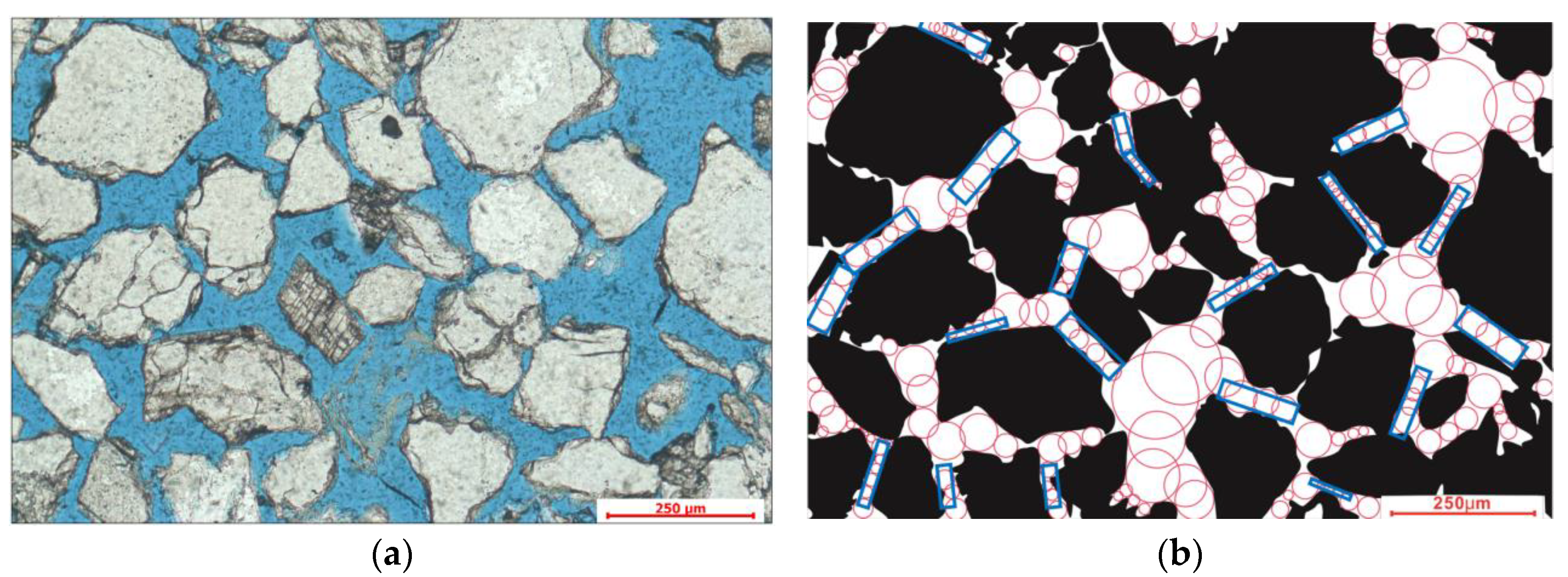
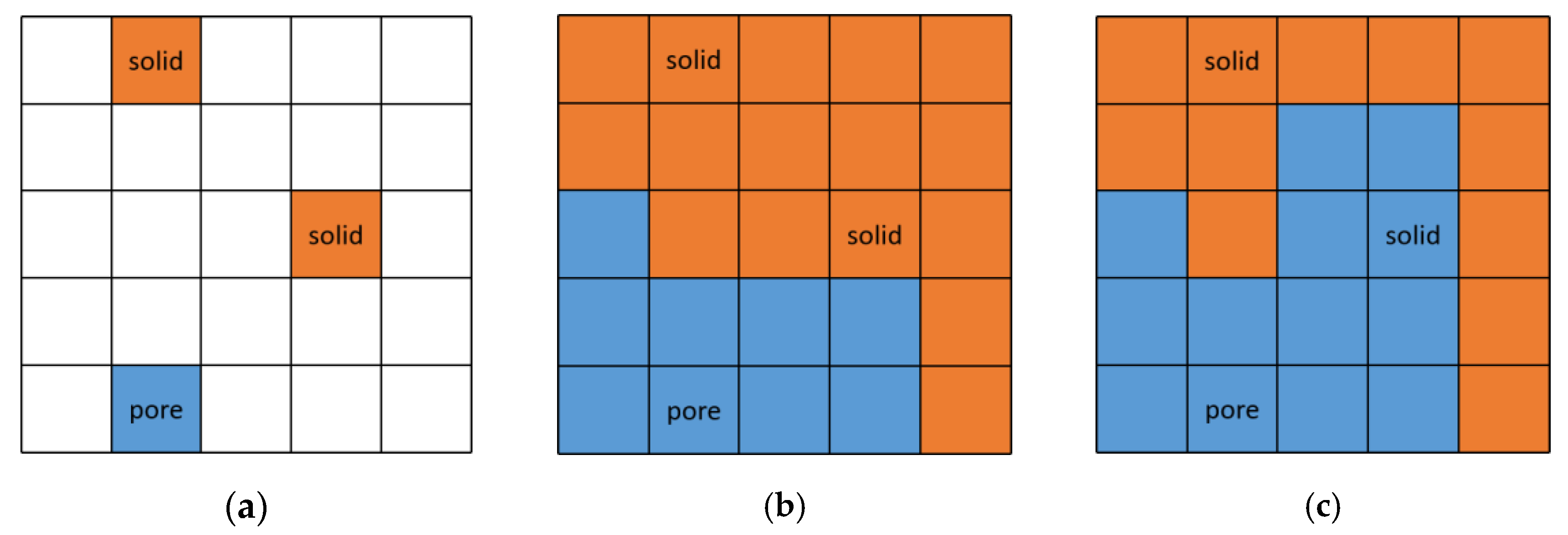
To establish a PNM using two-dimensional thin-section slices.

(ii)

To achieve fluid simulation using PNM and reduce the input dimensions of MLP with simulation results.

(iii)

To compare the predictive performance of the network after fluid calculation with that of the original network.

(iv)

To attempt to change the number of layers in the MLP to obtain the best prediction results.

2. Methodology

All following thin-section image analysis data are based on digital image analysis of porous media [30,31,32]. Generally speaking, the images obtained from SEM and Micro-CT are grayscale only. In such cases, a complete and accurate pore space can be obtained by using simple thresholding in an iterative method. However, thin-section images (Figure 1a) contain the colors red, green and blue (RGB), resulting in images with complex color particles for clay and cement, and strong color heterogeneity, with a blurry boundary. Therefore, accurate results cannot be obtained using traditional methods to segment the pore space in RGB images. We use an existing general algorithm to differentiate pores and grains. Firstly, the image is converted into the RGB color space; then, a color is selected to be extracted. In the RGB color space, the three primary colors are each represented by 255 levels. The next step is to traverse each nearby pixel, calculate the Euclidean distance between it and the target color, and select the nearest color as the extraction result. The color value of each pixel is replaced with the results obtained from the extracted image. It should be noted that the extracted results obtained using this algorithm are influenced by the chosen target color, so manual intervention is required for initial pore point selection. By repeatedly clicking on the possible pore range, all pores are selected. Therefore, it is necessary to make a selection based on the specific situation. In addition, after obtaining the pores, the maximum inscribed circle method is used to fill the pores in order to determine the average pore radius. Circles with continuously overlapping radii and smaller-than-average pore radius are replaced with rectangles. These rectangles are considered throats.

All of the subsequent thin-section image analysis data are based on the DIA technique for porous media [30,31,32]. Thin sections (Figure 1a) are color images in RGB format. They consist of complex-colored particles, clay, and cement, and exhibit strong color heterogeneity, resulting in blurred boundaries. Therefore, the methods traditionally used for segmenting pore space in RGB images may not yield accurate results.

We employed an existing general algorithm for segmenting pores and grains in the RGB images. Firstly, the image is converted into the RGB color space, and a specific color is selected for extraction. In the RGB color space, the three primary colors are each represented with 255 levels each. The next step involves traversing each nearby pixel, calculating the Euclidean distance between the pixel and the target color, and selecting the closest color as the extraction result. The color value of each pixel is replaced with the extraction result, resulting in the extracted image. It should be noted that the extraction results of this algorithm are influenced by the selected target color, and choosing different target colors may lead to variations in the extraction results. Therefore, the selection should be based on the specific circumstances. Furthermore, after obtaining the pores, the maximum inscribed circle method is applied to fill the pores and obtain the average pore radius. Circles with continuously overlapping radii that are smaller than the average pore radius are replaced with rectangles, and are considered throats.

In order to separate the coordinates of points with the same or similar color from the total body of pixels, a standard is given based on Euclidean distance in Equation (1), which is used to characterize the similarity between two points [33].

$$E_D=\sqrt{{(R-R_{x_o,y_o})}^2+{(G-G_{x_o,y_o})}^2+{(B-B_{x_o,y_o})}^2}$$

(1)

where the R, G, B represent the values of the red, green, and blue channels, respectively. x₀ and y₀ are the coordinates that have already been selected as pore pixel points. As subscripts, they indicate the RGB value of any selected pore part point. R, G, and B without subscripts represent the RGB color values of the point adjacent to x₀ and y₀. In Figure 1a, sky blue is assigned as the color representing pores, and any color in its vicinity within a Euclidean distance of 50 from sky blue is considered part of the pore. The method used to generate the maximum inscribed circles involves randomly distributing seeds inside the pores. Each seed generates a circle with a radius of 1 pixel. The radius of the circle is then iteratively increased, but it must not exceed the pore boundary. The center of the circle shifts as the radius increases. When none of the circles continue to change after iteration, they are sorted based on their radius. Larger circles absorb smaller or equal-sized circles that overlap with them by more than 80%.

The sample shown is a sandstone sample collected from a depth of over two thousand meters in the western South China Sea, with a porosity of 20% and a permeability of 80 mD. Figure 2b on the right shows circles representing the pores obtained using DIA software for maximum sphere operation. As depicted in Figure 2b, we employ small overlapping circles as the criterion for determining the presence of throats. Each circle corresponds to a sphere, and the distribution of circles represents the pore distribution. The rectangles cover relatively small and continuous circles, which are considered to be throats. The width of the rectangle corresponds to the throat width. Small circles refer to circles with a radius smaller than the mean radius. Throats are identified and marked with a blue rectangle, and their width and quantity distribution are automatically calculated. Subsequently, the information regarding pores and throats is subjected to statistical analysis (Figure 2b). All of the statistical information was gathered, and is presented in

Table 1. The pore and throat parameters of the thin section obtained through the DIA.

Pore and Throat Parameter	Include Data Content	Number of Parameters	Can be Used to Reconstruct PNM
Pore type	Pore type rank: 1~6	1	no
Lithology	Lithology rank: 1~14	1	no
2D porosity	Porosity %	1	yes
Average coordination number	Decimal number	1	yes
Reservoir code	Integer	1	no
Well number	Well name code: 1~2000	1	no
Tortuosity	Decimal number	1	yes
Pore shape factor distribution	Range (0~1.0)	13	yes
Average pore–throat ratio	Decimal number	1	yes
Max throat count	Integer	1	no
Pore diameter distribution	Range (2 μm~2000 μm)	40	yes
Throat diameter distribution	Range (2 μm~2000 μm)	40	yes
Coordination number distribution frequency	Range (0~8.0)	8	yes
Permeability	The same depth core analysis permeability	1	no

. In Table 1, the designation of pore types and lithology is performed manually, encompassing all the pores within the entire field of view.

We conducted thin-section image analysis on 40 core samples obtained from the Ying ge hai Basin and Pearl River Estuary Basin. The data presented in Table 1 represent the obtained results. We assigned codes from 1 to 6 to rank the pore types, including dissolution pores, micropores, interstitial pores, dissolution cavities, intergranular pores, and fissures. Similarly, we assigned codes to represent the lithology, following the sequence of boulder, cobble, pebble, granule, very coarse sand, coarse sand, medium sand, fine sand, very fine sand, coarse silt, medium silt, fine silt, very fine silt, and clay. The remaining twelve parameters, such as average coordination number, were calculated and generated by the image analysis software developed by Sichuan University, in accordance with the Standard for Image Analysis Method SY-T 6103-2019. Based on the thin-section image data, well test results, and laboratory core analysis results, we obtained 40 sets of thin-section permeability samples. Of these, we randomly selected 30 sets for training purposes, while the remaining 10 sets were used as test samples. Our initial attempt involved fitting the permeability using the classic MLP network. Throughout this process, we kept the samples unchanged while constantly modifying the number of layers and hidden nodes in the network, aiming to achieve a more stable network model. Detailed parameter information is provided in the following.

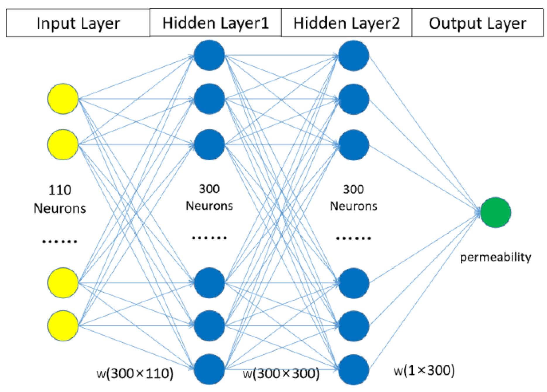
2.1. Classic MLP Network Method

Firstly, we attempted to input the 110-dimensional input and 1-dimensional output directly into the network as training samples without reducing the data dimensions. The network structure consisted of three layers, with the input layer containing 110 neurons. The data for the thin-section pore and throat characteristics were included in the output layer, representing the one-dimensional permeability value for supervised training. The number of neuron nodes in the hidden layer needed to be tested to determine the optimal number for achieving the best fitting effect. We experimented with a single hidden layer in the MLP network, ranging from 100 to 300 neurons, as shown in Figure 3. For each network type, the training process always involved gradient descent, terminating when the overall average relative error was less than 0.0000001 or after exceeding 1,000,000 iterations. We extracted pore and throat information from 600 thin-section images and selected 400 of them randomly as training samples. All data were normalized before being fed into the MLP network. The normalization process involved finding the maximum and minimum values of each parameter across all samples and then linearly mapping the parameter to the range of [0, 1]. It was observed that whether the activation function was Sigmoid or Tanh, similar training results were obtained.

During each training iteration, the pore and throat features of the image are fed into the input nodes, and forward propagation is performed. The weights are then updated after each iteration. Each batch consists of only one sample, and a cycle is carried out every 10 iterations to reduce the relative error of the network on a single sample. The initial learning rate is set to 0.001, and the learning rate is reduced by half at 20,000, 40,000, and 60,000 iterations. Upon completing the training process, the results are presented in Figure 4. Figure 4 shows that increasing the number of neurons will not improve the convergence of the relative error for training. In fact, even when the MLP network is expanded to two hidden layers, the convergence trend worsens. Generally, when the number of neurons in the hidden layer exceeds 100, the network tends to converge to an average relative error of approximately 0.00001 for the training samples. However, when the trained network is used to predict samples that were not included in the training set, the network does not exhibit satisfactory prediction performance. As training progresses, the percentage of the predicted results that are within a 10% error range is approximately 90%. Based on our existing data processing experience, it is likely that the sample data contain excessive noise and invalid data, leading to overfitting. This is especially true for the data related to pore and throat distribution, where a significant number of data points approach zero. Additionally, the same lithology, pore type, and permeability values correspond to multiple pore and throat distributions. Such sample data make it challenging to determine the key parameters during training.

We attempted to implement dropout during training to mitigate the issue of overfitting. The process of dropout involves randomly excluding certain neurons during each iteration. This operation allows the network layers to collaboratively adjust and rectify errors from the preceding layer, thereby enhancing the model’s robustness. However, the dropout technique did not yield the anticipated results. Although it expedited the training process, it did not significantly improve the predictability of the model.

In porous media, the increase in permeability resulting from the dominant channels is much more significant than the other parameters. This insight prompted us to explore a more effective approach for handling the data: transforming the thin section data into a representative 3D digital core and conducting fluid simulations to identify the crucial fluid channels. Considering the underlying logic, solely altering the network outcomes may not uncover the appropriate data relationships. While increasing the number of hidden layers may decrease the overall data error, it does not enhance the model’s generalization ability. Moreover, overfitting becomes a prominent issue during the dissemination process. In some cases, the prediction of untrained samples may even yield a permeability of zero. Therefore, it is necessary to incorporate fluid mechanics simulations to guide the training process.

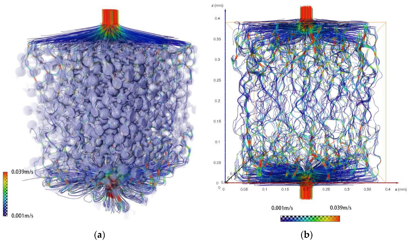
2.2. Fluid–MLP Network Method

It is essential to establish a three-dimensional digital core in order to facilitate fluid simulation and provide training data. The 3D digital core can be reconstructed using the PNM (Pore Network Model), which involves excavating spherical holes and connecting cylinders within the solid structure. The current prevalent method for constructing a pore network model is the maxima-ball algorithm [33,34,35]. This algorithm not only improves the speed of network extraction, but also ensures the accuracy of pore distribution and connectivity features in 3D space. The maxima-ball method relies on 3D data obtained from CT scanning. However, obtaining qualified CT scan samples is a complex process that requires sufficient time to generate accurate scan data. Generating the pore network model from the pore and throat data obtained from thin-section images instead could greatly reduce the difficulty and preparation time inherent in acquiring the pore network model.

Currently, commonly used computer simulation algorithms for sphere stacking include the sequence addition algorithm and the set rearrangement algorithm. The sequence addition algorithm fails to achieve a high stacking density and tends to create a more densely stacked structure in one direction compared to others. On the other hand, the set rearrangement algorithm overcomes the limitations of sequence addition, but results in changes to the sphere sizes. Additionally, the algorithm allows for overlap between spheres during the initial stages of stacking, which does not accurately represent real sphere stacking scenarios. The key focus of the algorithm is on reducing the overlap between spheres to within a specific range, generally leading to a high stacking density. We employ a new stacking method called sequential stacking based on collision radius in order to more effectively simulate the state of throat connections between porous spheres. In this method, the collision radius of the sphere is greater than the actual pore radius, since throats are necessary for connecting the spheres.

We reconstruct the Pore Network Model (PNM) from thin-section data by randomly stacking pore balls within a 400 μm × 400 μm × 400 μm cube. To estimate the sphere radius, we first generate a probability function based on the distribution of pore diameters. The stacking process involves free-falling spheres under the influence of gravity. The kinetic energy of each sphere is proportionally reduced during collision, leading to a stable state. The algorithm principle shown as Figure 5a,b can be summarized as follows: (1) Randomly construct an initial layer of stacked spheres at the bottom; (2) Create a new sphere P at a random position at the top. The collision radius of P is obtained by multiplying a random value R, generated by the aperture distribution function, by the tortuosity. Sphere P is then stacked under the influence of gravity; (3) Detect the collision between sphere P and the boundary or stacked spheres and bounce back with 50% energy reduction when this occurs. Once the kinetic energy of sphere P decreases below the threshold K, fix its position, and mark it as a stacked sphere. It will no longer be affected by gravity or move; (4) When it is not possible to generate a new sphere P in the entire space, use the throat radius distribution function to generate the throat radius r. Create a throat by connecting adjacent spheres with a cylinder of throat radius r, based on the coordination number. Dig out the spheres and cylinders within the solid and calculate the solid porosity. If the porosity does not meet the requirements, adjust it by using the throat length. If the porosity is lower than the expected value, reduce all throat lengths to (existing porosity/expected porosity × throat length) and return to step 1 to regenerate the model, and vice versa.

Once the 3D cube is reconstructed as shown in Figure 5, we employ the multi-point geostatistics method to verify whether this 3D model exhibits the same properties as the thin section [36,37]. We randomly select three points as a template and evaluate its matching probability in both transverse and longitudinal sections of the 3D model [38]. If the template’s matching probability follows the same distribution as the thin section in different slice directions, this confirms that the 3D model and the 2D model share the same attributes [39]. Figure 6 presents the specific template matching method. First, we generate a template consisting of three points, as depicted in Figure 6a. We randomly examine the entire slice and calculate the matching probability of the template distribution [40,41]. For each template, we randomly select 100 points in transverse and longitudinal sections to assess whether the points meet the template requirements. The final matching probability of a randomly generated template is derived from the equation (probability = Matched case/All case), as shown in Figure 6b,c. The probabilities presented in Figure 7 have been normalized, and the sum of all probabilities amounts to 100%. If the average difference in matching probability between the 3D and thin-section templates is less than 30%, we consider the established 3D model capable of representing the original thin-section image. If the overall does not match the templates, we randomly rebuild the entire stacking process until it matches the templates. In Figure 7, we perform 100 checks per template [42,43,44,45].

Finally, we generated two representatives of PNM as shown in Figure 8. Then, we used the lattice Boltzmann method (LBM) to simulate the permeability of this pore network model. In the LBM, the motion of fluid particles needs to be mapped onto the velocity space. In the D3Q19 model, each direction is assigned a specific discrete velocity, as in Equation (2):

$${\xi }_{\mathrm{velocity}}=\left\{\begin{array}{ccccccccccccccccccc}0& 1& -1& 0& 0& 0& 0& 1& -1& 1& -1& 1& -1& 1& -1& 0& 0& 0& 0\\ 0& 0& 0& 1& -1& 0& 0& 1& -1& -1& 1& 0& 0& 0& 0& 1& -1& 1& -1\\ 0& 0& 0& 0& 0& 1& -1& 0& 0& 0& 0& 1& -1& -1& 1& 1& -1& -1& 1\end{array}\right.$$

(2)

where each column of the formula matrix represents an independent velocity direction vector, which points to another grid site in the mesh [12,46,47,48,49].

The evolution equation of the distribution function corresponding to each discrete velocity is as follows:

$$f_{}(x+{\xi }_{\mathrm{velocity}}{\delta }_t,t+{\delta }_t)-f_{}(x,t)=-\frac{1}{{\tau }_{\mathrm{velocity}}}(f_{}(x,t)-f_{}^{eq}(x,t))$$

(3)

where the subscript “velocity” represents the fact that this evolution equation is only for a propagator moving in the velocity field. ξ is the discrete velocity, x is the position coordinates of each distribution function f. The f(x, t) signifies a particle density distribution function over the space of microscopic particle velocities ξ. δ_t is the lattice unit time. The τ velocity is the average collision time. For the same fluid, τ is a constant value, and here τ = 1. The superscript “eq” is for the equilibrium distribution function. For each site, propagator density and velocity can be obtained by:

$${\rho }_{\mathrm{propagator}}^{}={\displaystyle \sum _0^{18}\left(f\right)}$$

(4)

$$u_{\mathrm{macro}}^{}=w_a{\displaystyle \sum _0^{18}\left(f_{}\right)}$$

(5)

where ρ_propagator is the simulated density at a site, and u_macro is the water velocity at a site before collision. The value of weight w_a is:

$$\left\{\begin{array}{l}{w}_0=1/3\\ w_{1\dots 6}=1/18\\ w_{7\dots 18}=1/36\end{array}\right.$$

(6)

When the macro velocity is not zero, the propagation density in each direction can be calculated using the following equation:

$$f_a^{eq}=w_a\rho \left(1+\frac{c_a^{}\cdot u}{c_s^2}+\frac{{\left(c_a^{}\cdot u\right)}^2}{2c_s^4}+\frac{u\cdot u}{2c_s^2}\right)$$

(7)

where w_i is the weight coefficient in Equation (6). The c² = 3c_s², c_s is the sound velocity of the lattice. For the same fluid, c_s is a constant value; here, we let 3c_s² = 1. These coefficients can be solved using the following restriction conditions:

$$\left\{\begin{array}{l}{\displaystyle \sum _0^{18}{w}_a}=1\\ {\displaystyle \sum _0^{18}{w}_a}{c}_a=0\\ {\displaystyle \sum _0^{18}{w}_a}{c}_{a\alpha }{c}_{a\beta }=Q{c}^2{\delta }_{\alpha \beta }\\ c=\frac{{\delta }_x}{{\delta }_t}=\frac{{\delta }_y}{{\delta }_t}=\frac{{\delta }_z}{{\delta }_t}\end{array}\right.$$

(8)

where δ_t is the lattice unit of time, and δ_x, δ_y, and δ_z the lattice units of space in the X-, Y-, and Z-axes. The correspondence we use is that one lattice length unit corresponds to 1 μm in real life. According to the Chapman–Enskog expansion, the permeability of the fluid is proportional to its velocity in a specific direction. For the same fluid, Q is a constant value. Here, we let Q = 1. In the permeability simulation, the fluid’s movement speed is slower, the streamlines are smoother, the fluid’s diffusivity is stronger, and the turbulence phenomenon of the fluid is less. Additionally, the viscous force of the fluid has a greater impact on the fluid, so the fluid’s movement state is more stable and the fluid’s flow stability is higher. Therefore, we assume that the fluid exhibits a low Reynolds number characteristic, and we can use the fluid-viscosity-related τ as an invariant for unit conversion between the lattice unit system and the actual unit system in space and time. This conversion allows us to obtain a simulated permeability that contains information in 110 + 1 (permeability) dimensions. The simulated permeability (Equation (9)) and the real permeability have the same characteristics, that is, when the dominant channel is wider, the permeability becomes greater, but due to differences in sampling methods, they are not exactly equal.

$$permeability=\left(\sum _{i=0}^{{400}^3\left(lattice\right)}{u}_X\right)/\left({400}^3\right)$$

(9)

Once the simulated permeability is obtained, it encompasses 112 dimensions of information. However, for sample training, we only utilize the following six dimensions as input: pore type rank, lithology rank, average pore–throat ratio, 2D porosity, average throat diameter, and simulated permeability. When we employ this six-dimensional input, we refer to it as the Fluid–MLP network within the MLP network. The process of using the LBM to simulate fluid in the generated porous network model is depicted in Figure 9. In the simulation, a pressure difference of 4 MPa is applied at both ends of the rock core, mimicking typical experiments for measuring rock permeability. This allows for the unidirectional flow of a single fluid (i.e., water) through the network model. Each voxel of the model has dimensions of μm × 1 μm × 1 μm, and the mean pore radius is 13 μm. The LBM implementation employs the D₃Q₁₉ scheme with fully bounce-back boundary conditions. By utilizing Shan-Chen force, a volume force is directly exerted on the fluid throughout the core of the model. The acceleration of each grid is equal to the pressure gradient multiplied by the cross-sectional area of each cell [50]. Due to this acceleration, the fluid initiates flow until it reaches a stable flow rate, which occurs after approximately 100 steps. At this point, we generate a streamline map of the velocity field, where the color represents the velocity magnitude, and the direction of the streamlines indicates the velocity direction. We first validated the LBM described in the paper “Microstructure-based modeling of permeability of cementitious materials using multiple-relaxation-time lattice Boltzmann method”, and then used conversion coefficients to convert the dimensionless velocity into meters per second. The maximum flow velocity obtained was 0.03922932 m/s, as illustrated by the red section in Figure 9b. According to the calculation, the permeability of the pore model reached 21 millidarcies.

3. Results and Discussion

Compared with the original MLP, the Fluid–MLP removes some input parameters that are not directly or linearly related to the outputs. We performed a fluid simulation, and used the permeability simulated using the 3D model as the input. The results demonstrate that fluid simulation can indeed improve the stability of the prediction.

Table 2. Comparison of Fluid–MLP and the original MLP where CPU frequency is 5.2 GHz.

Network Structure	Number of Hidden Nodes	Training Average Relative Error (after 1 × 107 iterations)	Proportion of Correct Predictions (Error within ±10% Measured Permeability)
Original MLP	300	<1 × 10−5	89% (training time 671s)
Original MLP	300 + 300	<1 × 10−5	90% (training time 1950s)
Fluid–MLP	100	<1 × 10−6	93% (training time 101s)
Fluid–MLP	300	<1 × 10−6	93% (training time 324s)
Fluid–MLP	300 + 300	<1 × 10−6	94% (training time 1560s)

shows that the Fluid–MLP network has obviously better prediction performance than the original network.

The Fluid–MLP workflow allows for the processing of various types of pore-throat characteristic data and enables faster machine learning. To determine whether there are reducible components among the remaining input parameters, we sequentially excluded the inputs of pore type, lithology, 2D porosity, average pore–throat ratio, and average throat diameter. We continued to use the aforementioned samples for testing, and the results are presented in

Table 3. Comparison of prediction performance when dropping one input parameter.

Dropped Parameter	Proportion of Correct Predictions with All 110 and with 6 Parameters	Proportion of Correct Predictions after Dropping 1 Parameter	Difference with 6 Parameters
Pore type rank	89%, 93%	70%	23%
Lithology rank	89%, 93%	56%	37%
2D porosity	89%, 93%	84%	9%
Average pore–throat ratio	89%, 93%	70%	24%
Average throat diameter	89%, 93%	78%	15%

. Regardless of which input was excluded, the prediction performance was significantly deteriorated. Manual calibration parameters, such as pore type and lithology, play a crucial role in this context. It is likely that rock pores exhibit different fluid characteristics even under the same maximum spherical distribution due to the influence of the deposition environment and method. Additionally, the pores may contain non-miscible fluids, which can also impact the overall permeability prediction. The pore network model, being a simplified approximation method for representing real pore structures, overlooks certain details that are captured by the pore type and lithology parameters. It is for this reason that the remaining five parameters in Table 3 cannot be further reduced.

After fixing the network model’s input to six parameters, we conducted a more extensive comparison of prediction performance. We used the data from 1000 thin sections from eight wells in two basins as training samples to predict the permeability of another 800 thin sections from the same wells. The measured permeability, obtained from core analysis and well testing, represents different scales and may not correspond exactly in terms of depth. Therefore, we relaxed the comparison criteria. Any predicted permeability within a 10% absolute difference from the measured permeability was considered correct. The results in

Table 4. Large sample training and prediction results.

Well Number	Basin Number	Number of Samples	Proportion of Correct Predictions
1–2	1	287	92%
3–4	1	210	92%
5–6	2	181	90%
7–8	2	322	94%

and Figure 10 indicate that the model demonstrates consistent prediction ability following training with both large and small samples. However, due to the inclusion of reservoir and well differentiation, the model still relies on geological knowledge. It is essential to introduce new regional samples when the model is applied to new regions.

4. Conclusions

This paper presents the Fluid–MLP method, which is a new technical workflow for estimating 3D permeability from 2D thin-section images. We extracted 110 pore-throat characteristic parameters from 2D thin slices and constructed a pore network model using the pore size parameters to simulate permeability. By training the Fluid–MLP model using the simulated permeability as the input, we made several attempts to change the network structure and obtained the following main conclusions:

1.

It is proposed that the characteristic parameters obtained from two-dimensional reservoir rock thin-section images can be used to construct an equivalent PNM.

2.

A drop-out input experiment was conducted using the Fluid–MLP network model, in which the input dimensions were reduced from 112 to 6. The average accuracy of permeability prediction on the training samples was around 92%. The reduced number of input dimensions and hidden layer neurons significantly improved training time efficiency, with a slight improvement in accuracy.

3.

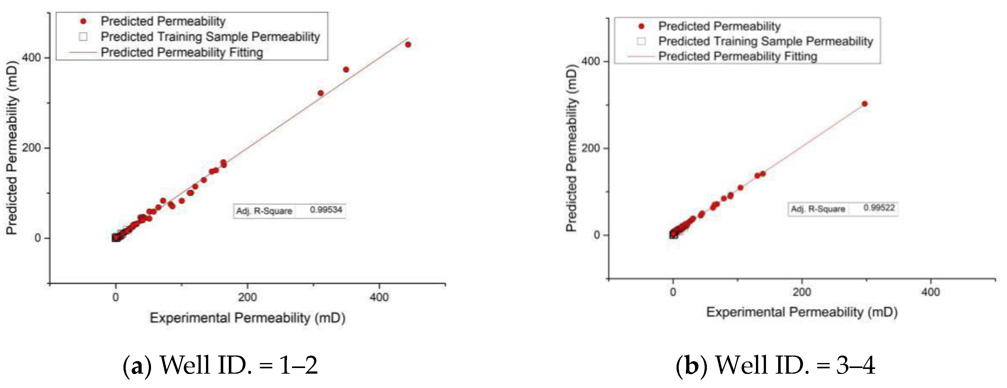
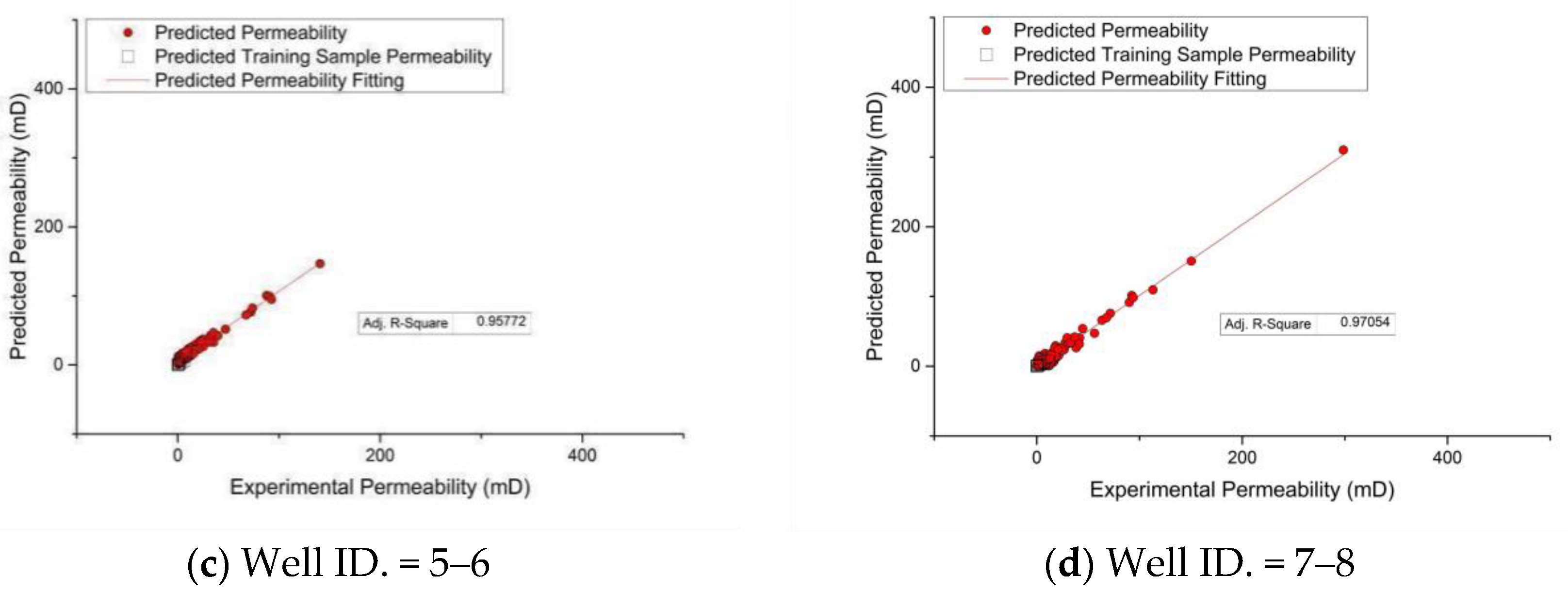
Compared to the original MLP network, the Fluid–MLP network achieved an average improvement in prediction accuracy of approximately 4%. We also compared different training sample sizes and found that the Fluid–MLP network outperformed the original MLP network by over 1% in terms of prediction accuracy.

4.

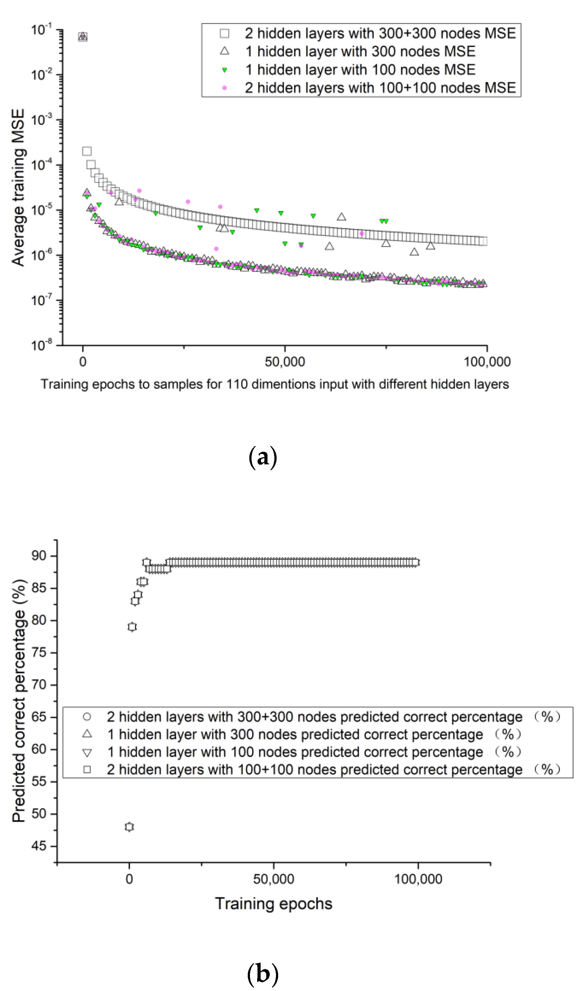
Our comparison with the results obtained when adding hidden layers showed that the addition of hidden layers did not effectively improve the original MLP network or the prediction accuracy of the Fluid–MLP network.

Because the results described above only cover a small fraction of the different rock types, and it is still necessary to retrain in different regions; therefore, this method still leaves a lot of room for improvement. One direction for the future would be to use autoencoder networks to automatically extract key information, avoiding the interference of different regions on the results.

References

1. Øren, P.-E.; Bakke, S. Process Based Reconstruction of Sandstones and Prediction of Transport Properties. Transp. Porous Media 2002, 46, 311–343. [Google Scholar] [CrossRef]
2. Miele, R.; Grana, D.; Varella, L.E.S.; Barreto, B.V.; Azevedo, L. Iterative geostatistical seismic inversion with rock-physics constraints for permeability prediction. Geophysics 2023, 88, M105–M117. [Google Scholar] [CrossRef]
3. Raghavan, R. Some observations on the scale dependence of permeability by pumping tests. Water Resour. Res. 2006, 42. [Google Scholar] [CrossRef]
4. Heap, M.J.; Kennedy, B.M. Exploring the scale-dependent permeability of fractured andesite. Earth Planet. Sci. Lett. 2016, 447, 139–150. [Google Scholar] [CrossRef]
5. Shabani, M.; Ghanizadeh, A.; Clarkson, C.R. Gas relative permeability evaluation in tight rocks using rate-transient analysis (RTA) techniques. Mar. Pet. Geol. 2023, 152, 106207. [Google Scholar] [CrossRef]
6. Chen, X.; Zhao, X.; Tahmasebi, P.; Luo, C.; Cai, J. NMR-data-driven prediction of matrix permeability in sandstone aquifers. J. Hydrol. 2023, 618, 129147. [Google Scholar] [CrossRef]
7. Medici, G.; West, L.J. Reply to discussion on ‘Review of groundwater flow and contaminant transport modelling approaches for the Sherwood Sandstone aquifer, UK; insights from analogous successions worldwide’ by Medici and West (QJEGH, 55, qjegh2021-176). Q. J. Eng. Geol. Hydrogeol. 2023, 56, qjegh2022-097. [Google Scholar] [CrossRef]
8. Martyushev, D.A.; Ponomareva, I.N.; Chukhlov, A.S.; Davoodi, S.; Osovetsky, B.M.; Kazymov, K.P.; Yang, Y. Study of void space structure and its influence on carbonate reservoir properties: X-ray microtomography, electron microscopy, and well testing. Mar. Pet. Geol. 2023, 151, 106192. [Google Scholar] [CrossRef]
9. Dong, S.; Zeng, L.; Xu, C.; Dowd, P.; Gao, Z.; Mao, Z.; Wang, A. A novel method for extracting information on pores from cast thin-section images. Comput. Geosci. 2019, 130, 69–83. [Google Scholar] [CrossRef]
10. Rabbani, A.; Assadi, A.; Kharrat, R.; Dashti, N.; Ayatollahi, S. Estimation of carbonates permeability using pore network parameters extracted from thin section images and comparison with experimental data. J. Nat. Gas Sci. Eng. 2017, 42, 85–98. [Google Scholar] [CrossRef]
11. Chen, X.; Yao, G.; Luo, C.; Jiang, P.; Cai, J.; Zhou, K.; Herrero-Bervera, E. Capillary pressure curve determination based on a 2-D cross-section analysis via fractal geometry: A bridge between 2-D and 3-D pore structure of porous media. J. Geophys. Res. Solid Earth 2019, 124, 2352–2367. [Google Scholar] [CrossRef]
12. Keehm, Y.; Mukerji, T.; Nur, A. Permeability prediction from thin sections: 3D reconstruction and Lattice-Boltzmann flow simulation. Geophys. Res. Lett. 2004, 31, L04606. [Google Scholar] [CrossRef]
13. Okabe, H.; Blunt, M.J. Prediction of permeability for porous media reconstructed using multiple-point statistics. Phys. Rev. E 2004, 70, 066135. [Google Scholar] [CrossRef] [PubMed]
14. Liu, M.; Ahmad, R.; Cai, W.; Mukerji, T. Hierarchical Homogenization With Deep-Learning-Based Surrogate Model for Rapid Estimation of Effective Permeability From Digital Rocks. J. Geophys. Res. Solid Earth 2023, 128, e2022JB025378. [Google Scholar] [CrossRef]
15. Neto IA, L.; Misságia, R.M.; Ceia, M.A.; Archilha, N.L.; Oliveira, L.C. Carbonate pore system evaluation using the velocity–porosity–pressure relationship, digital image analysis, and differential effective medium theory. J. Appl. Geophys. 2014, 110, 23–33. [Google Scholar] [CrossRef]
16. He, J.; Ding, W.; Li, A.; Sun, Y.; Dai, P.; Yin, S.; Chen, E.; Gu, Y. Quantitative microporosity evaluation using mercury injection and digital image analysis in tight carbonate rocks: A case study from the Ordovician in the Tazhong Palaeouplift, Tarim Basin, NW China. J. Nat. Gas Sci. Eng. 2016, 34, 627–644. [Google Scholar] [CrossRef]
17. Mollajan, A.; Ghiasi-Freez, J.; Memarian, H. Improving pore type identification from thin section images using an integrated fuzzy fusion of multiple classifiers. J. Nat. Gas Sci. Eng. 2016, 31, 396–404. [Google Scholar] [CrossRef]
18. Pal, A.K.; Garia, S.; Ravi, K.; Nair, A.M. Pore scale image analysis for petrophysical modelling. Micron 2022, 154, 103195. [Google Scholar] [CrossRef]
19. Payton, R.L.; Chiarella, D.; Kingdon, A. The upper percolation threshold and porosity–permeability relationship in sandstone reservoirs using digital image analysis. Sci. Rep. 2022, 12, 11311. [Google Scholar] [CrossRef]
20. Rabbani, A.; Fernando, A.M.; Shams, R.; Singh, A.; Mostaghimi, P.; Babaei, M. Review of Data Science Trends and Issues in Porous Media Research With a Focus on Image-Based Techniques. Water Resour. Res. 2021, 57, e2020WR029472. [Google Scholar] [CrossRef]
21. Ghiasi-Freez, J.; Soleimanpour, I.; Kadkhodaie-Ilkhchi, A.; Ziaii, M.; Sedighi, M.; Hatampour, A. Semi-automated porosity identification from thin section images using image analysis and intelligent discriminant classifiers. Comput. Geosci. 2012, 45, 36–45. [Google Scholar] [CrossRef]
22. Zaitoun, N.M.; Aqel, M.J. Survey on Image Segmentation Techniques. Procedia Comput. Sci. 2015, 65, 797–806. [Google Scholar] [CrossRef]
23. Tarabalka, Y.; Chanussot, J.; Benediktsson, J.A. Segmentation and classification of hyperspectral images using watershed transformation. Pattern Recognit. 2010, 43, 2367–2379. [Google Scholar] [CrossRef]
24. Zhao, F.; Liu, H.; Fan, J. A multiobjective spatial fuzzy clustering algorithm for image segmentation. Appl. Soft Comput. 2015, 30, 48–57. [Google Scholar] [CrossRef]
25. Pun, T. A new method for grey-level picture thresholding using the entropy of the histogram. Signal Process. 1980, 2, 223–237. [Google Scholar] [CrossRef]
26. Izadi, H.; Sadri, J.; Mehran, N.A. A new intelligent method for minerals segmentation in thin sections based on a novel incremental color clustering. Comput. Geosci. 2015, 81, 38–52. [Google Scholar] [CrossRef]
27. Chen, X.; Yao, G. An improved model for permeability estimation in low permeable porous media based on fractal geometry and modified Hagen-Poiseuille flow. Fuel 2017, 210, 748–757. [Google Scholar] [CrossRef]
28. Zhang, M.; Ye, G.; van Breugel, K. Microstructure-based modeling of permeability of cementitious materials using multiple-relaxation-time lattice Boltzmann method. Comput. Mater. Sci. 2013, 68, 142–151. [Google Scholar] [CrossRef]
29. Al-Mahrooqi, S.; Grattoni, C.; Muggeridge, A.; Zimmerman, R.; Jing, X. Pore-scale modelling of NMR relaxation for the characterization of wettability. J. Pet. Sci. Eng. 2006, 52, 172–186. [Google Scholar] [CrossRef]
30. Rabbani, A.; Jamshidi, S. Specific surface and porosity relationship for sandstones for prediction of permeability. Int. J. Rock Mech. Min. Sci. 2014, 71, 25–32. [Google Scholar] [CrossRef]
31. Rabbani, A.; Jamshidi, S.; Salehi, S. An automated simple algorithm for realistic pore network extraction from micro-tomography images. J. Pet. Sci. Eng. 2014, 123, 164–171. [Google Scholar] [CrossRef]
32. Houston, A.N.; Schmidt, S.; Tarquis, A.M.; Otten, W.; Baveye, P.C.; Hapca, S.M. Effect of scanning and image reconstruction settings in X-ray computed microtomography on quality and segmentation of 3D soil images. Geoderma 2013, 207–208, 154–165. [Google Scholar] [CrossRef]
33. Arand, F.; Hesser, J. Accurate and efficient maximal ball algorithm for pore network extraction. Comput. Geosci. 2017, 101, 28–37. [Google Scholar] [CrossRef]
34. Al-Kharusi, A.S.; Blunt, M.J. Network extraction from sandstone and carbonate pore space images. J. Pet. Sci. Eng. 2007, 56, 219–231. [Google Scholar] [CrossRef]
35. Aghaei, A.; Piri, M. Direct pore-to-core up-scaling of displacement processes: Dynamic pore network modeling and experimentation. J. Hydrol. 2015, 522, 488–509. [Google Scholar] [CrossRef]
36. Politis, M.; Kikkinides, E.; Kainourgiakis, M.; Stubos, A. A hybrid process-based and stochastic reconstruction method of porous media. Microporous Mesoporous Mater. 2008, 110, 92–99. [Google Scholar] [CrossRef]
37. Liu, X.; Sun, J.; Wang, H. Reconstruction of 3-D digital cores using a hybrid method. Appl. Geophys. 2009, 6, 105–112. [Google Scholar] [CrossRef]
38. Zhao, X.; Yao, J.; Yi, Y. A new stochastic method of reconstructing porous media. Transp. Porous Media 2006, 69, 1–11. [Google Scholar] [CrossRef]
39. Hajizadeh, A.; Safekordi, A.; Farhadpour, F.A. A multiple-point statistics algorithm for 3D pore space reconstruction from 2D images. Adv. Water Resour. 2011, 34, 1256–1267. [Google Scholar] [CrossRef]
40. Ju, Y.; Huang, Y.; Zheng, J.; Qian, X.; Xie, H.; Zhao, X. Multi-thread parallel algorithm for reconstructing 3D large-scale porous structures. Comput. Geosci. 2017, 101, 10–20. [Google Scholar] [CrossRef]
41. Wu, K.; Nunan, N.; Crawford, J.W.; Young, I.M.; Ritz, K. An efficient Markov chain model for the simulation of heterogeneous soil structure. Soil Sci. Soc. Am. J. 2004, 68, 346–351. [Google Scholar] [CrossRef]
42. Quiblier, J.A. A new three-dimensional modeling technique for studying porous media. J. Colloid Interface Sci. 1984, 98, 84–102. [Google Scholar] [CrossRef]
43. Tahmasebi, P.; Hezarkhani, A.; Sahimi, M. Multiple-point geostatistical modeling based on the cross-correlation functions. Comput. Geosci. 2012, 16, 779–797. [Google Scholar] [CrossRef]
44. Straubhaar, J.; Walgenwitz, A.; Renard, P. Parallel Multiple-Point Statistics Algorithm Based on List and Tree Structures. Math. Geosci. 2013, 45, 131–147. [Google Scholar] [CrossRef]
45. Strebelle, S. Conditional Simulation of Complex Geological Structures Using Multiple-Point Statistics. J. Int. Assoc. Math. Geol. 2002, 34, 1–21. [Google Scholar] [CrossRef]
46. Bakhshian, S.; Hosseini, S.A.; Shokri, N. Pore-scale characteristics of multiphase flow in heterogeneous porous media using the lattice Boltzmann method. Sci. Rep. 2019, 9, 3377. [Google Scholar] [CrossRef]
47. Tölke, J. Lattice Boltzmann simulations of binary fluid flow through porous media. Philos. Trans. R. Soc. A Math. Phys. Eng. Sci. 2002, 360, 535–545. [Google Scholar] [CrossRef] [PubMed]
48. Ahrenholz, B.; Tölke, J.; Lehmann, P.; Peters, A.; Kaestner, A.; Krafczyk, M.; Durner, W. Prediction of capillary hysteresis in a porous material using lattice-Boltzmann methods and comparison to experimental data and a morphological pore network model. Adv. Water Resour. 2008, 31, 1151–1173. [Google Scholar] [CrossRef]
49. Küntz, M.; Mareschal, J.C.; Lavallée, P. Numerical estimation of electrical conductivity in saturated porous media with a 2-D lattice gas. Geophysics 2000, 65, 766–772. [Google Scholar] [CrossRef]
50. Andrä, H.; Combaret, N.; Dvorkin, J.; Glatt, E.; Han, J.; Kabel, M.; Keehm, Y.; Krzikalla, F.; Lee, M.; Madonna, C.; et al. Digital rock physics benchmarks—Part I: Imaging and segmentation. Comput. Geosci. 2013, 50, 25–32. [Google Scholar] [CrossRef]
Figure 1. Thin-section color image (a) and pore acquisition (pores correspond to blue parts); (b) Binary image (pores correspond to white parts).
Energies 16 06976 g001
Figure 2. Randomly generate maximum inscribed circles and merge overlapping parts. (a) Injecting blue resin ground thin-sections. (b) Generating channels through consecutive small circles.
Energies 16 06976 g002
Figure 3. The original MLP network diagram for thin-section pore and throat characterics.
Energies 16 06976 g003
Figure 4. Influence of the number of hidden layer nodes on the MLP network. (a) Increasing hidden layer nodes does not necessarily improve training performance. (b) Simply changing the network structure cannot significantly improve predictive ability.
Energies 16 06976 g004
Figure 5. 3D model reconstruction process from thin section pore and throat characteristics where the sphere inside the red box represents the newly generated sphere. (a) Randomly generate balls and let them fall to the position with the lowest potential energy; (b) Place the latest ball at the highest position and slide under the action of gravity.
Energies 16 06976 g005
Figure 6. Multi-point geostatistical method for checking whether the 3D model and the thin-section image match. (a) Randomly create template; (b) Matched template case in slice area; (c) Not matched template case in slice area. Orange represents solid voxels generated, while blue represents fluid voxels generated.
Energies 16 06976 g006
Figure 7. Comparison of reconstructed 3D model and thin-section image statistics.
Energies 16 06976 g007
Figure 8. PNM generated using extracted pore and throat radius distribution. (a) Average pore radius = 13.2 μm; (b) Average pore radius = 9.2 μm.
Energies 16 06976 g008
Figure 9. The process of calculating permeability using the lattice Boltzmann method. (a) Streamlines are obtained by tracing the velocity field; (b) The permeability is obtained by calculating the flow rate passing through both ends.
Energies 16 06976 g009
Figure 10. Comparison of experimental and predicted permeability from multiple wells.
Energies 16 06976 g010aEnergies 16 06976 g010b