Abstract
Energy usage in robotic applications is rapidly increasing as industrial robot installations grow. This research introduces a novel approach, using the rapidly exploring random tree (RRT)-based scheme for optimizing the robot’s motion planning and minimizing energy consumption. Sampling-based algorithms for path planning, such as RRT and its many other variants, are widely used in robotic motion planning due to their efficiency in solving complex high-dimensional problems efficiently. However, standard versions of these algorithms cannot guarantee that the generated trajectories are always optimum and mostly ignore the energy consumption in robotic applications. This paper proposes an energy-efficient industrial robotics motion planning approach using the novel flight cost-based RRT (FC-RRT*) algorithm in pick-and-place operation to generate nodes in a predetermined direction and then calculate energy consumption using the circle point method. After optimizing the motion trajectory, power consumption is computed for the rotary axes of a six degree of freedom (6DOF) serial type of industrial robot using the work–energy hypothesis for the rotational motion of a rigid body. The results are compared to the traditional RRT and RRT* (RRT-star) algorithm as well as the kinematic solutions. The experimental results of axis indexing tests indicate that by employing the sampling-based FC-RRT* algorithm, the robot joints consume less energy (1.6% to 16.5% less) compared to both the kinematic solution and the conventional RRT* algorithm.
1. Introduction
In recent years, industrial robots have been increasingly introduced for small, low-volume production of multi-items. With a shortage of human resources, there is a need to automate complex transportation and production activities, such as pick-and-place operations in assembly and inspections using robotic systems to reduce manual labor. Various efforts have been made to transfer these tasks to industrial robots. However, the energy consumption in those robotic applications is growing rapidly. Operating industrial robots efficiently within limited space requires energy-efficient and conflict-free motion and trajectory planning, which is a critical concern. In the field of automation, particularly in robotic applications, precise motion planning and trajectory computation are of paramount importance.
Robots and automated devices operate at certain speeds to achieve shorter manufacturing periods. However, these operating speeds can impact the precision and repeatability of the motion trajectory, as they require intense actions from the robot’s joint actuators and the robot controller [1]. Researchers have focused on developing robot motion planning and trajectory generation algorithms that can be implemented at designated speeds while ensuring the safety of the robot [2,3]. Motion planning methods enable the robot to navigate along a geometric path, starting from an initial start position and reaching a final goal position while passing through predefined positions in either the robot’s configuration space (C-space) or operating space. On the other hand, trajectory planning algorithms follow a given geometric path and provide time information. Trajectory planning algorithms play a vital role in robotics as they influence not only the kinematic properties of the motion but also dynamic factors such as torque, gravity effects, friction, and so on [1,4].
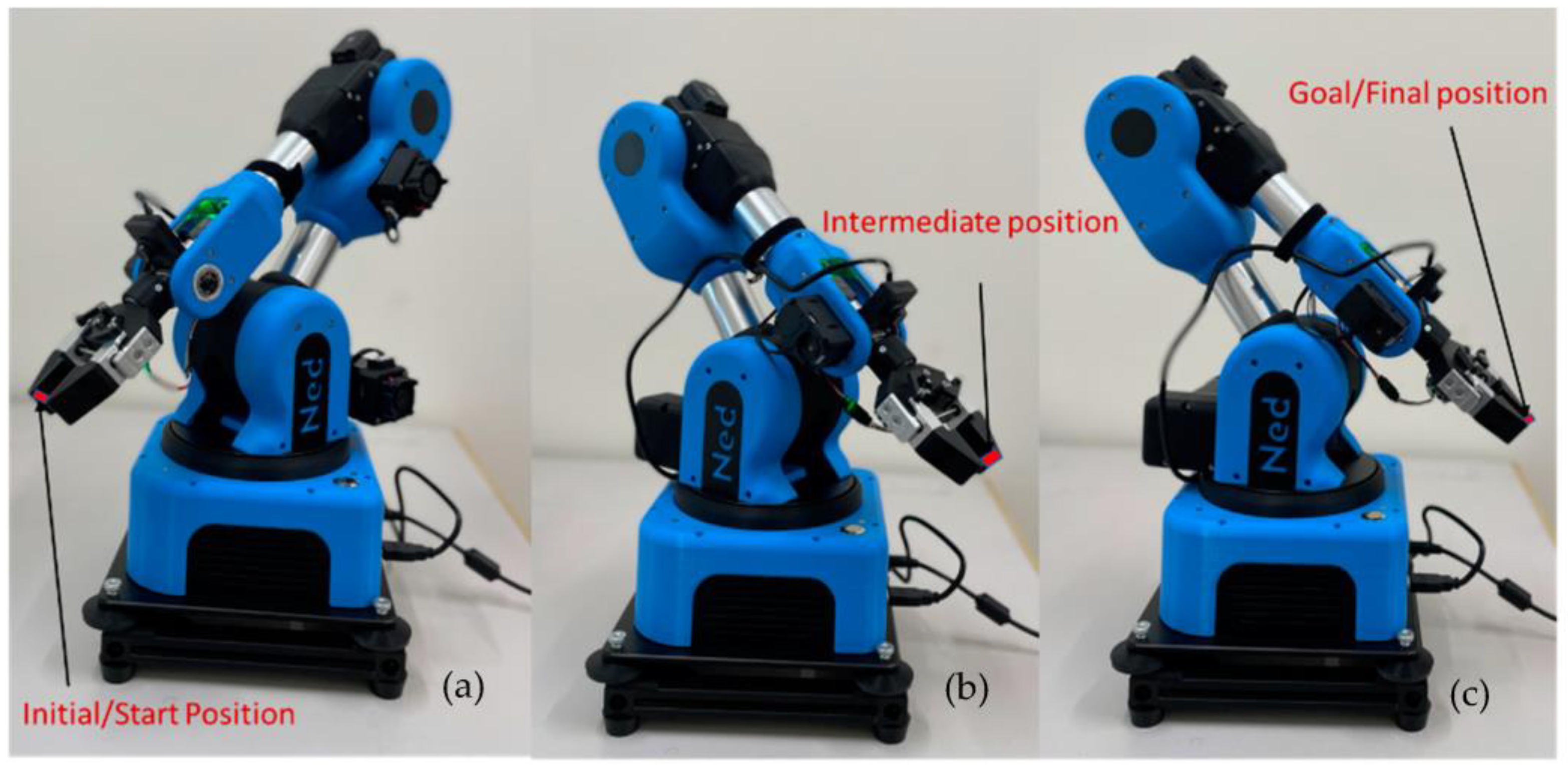
Furthermore, the growing demand for flexible robotic applications in dynamic manufacturing environments requires a growing number of manufacturing assembly resources. However, automated assembly systems like robotic manufacturing systems usually have limited flexibility due to the significant programming effort required to define robot trajectories from a start position to an end position, passing through intermediate positions as illustrated in Figure 1 for a 6DOF serial robot. Traditionally, skilled robot operators spend considerable time optimizing robotic operation paths for each specific application using conventional programming methods, typically referred to as robot teaching [5]. In robot teaching, intermediate positions between the start and goal positions are manually recorded by sequentially moving the robot to each position using the teach pendant, which is a time-consuming process. The robot’s final path is then generated by connecting the recorded positions using a robot controller, which moves across all the positions while considering the robot’s joint dynamics. The quality of the final trajectory heavily relies on the recorded positions and the experience of the robot operator.

Figure 1.
A robot with 6DOF configuration in pick-and-place operation in its (a) initial position through (b) intermediate position to (c) goal position. Please see Table 1.
Automatic path planning in robotics aims to determine how a robot can move from its initial to its final position, with a primary focus on collision avoidance. Over the past two decades, researchers have devoted significant efforts to achieving optimal motion trajectories through various approaches, aiming to minimize the cost or the time required to execute the robotic operation. For example, Chettibi et al. [6] created an electromechanical model of a series manipulator to find the optimal trajectory from the initial to the final position that satisfies the electromechanical constraints. Even in simple cases, computing optimal motion plans is challenging due to obstacles in the robot’s C-space [1,2,3,7].
Therefore, to achieve offline robot programming and address computational challenges, it is necessary to optimize the motion planning trajectory by applying effective algorithms to the robot while in operation. In this research, we apply a novel motion planning algorithm (FC-RRT*) for an industrial robot (as shown in Figure 1) using the circle point method, which considers energy consumption during object picking and placing. We compare this novel motion planning algorithm to traditional algorithms and robot kinematics solutions. Furthermore, to the best of the authors’ knowledge, this circle point method has not been used to optimize energy consumption during motion planning in prior studies.
Conventional motion and path planning methods neglect the reduction of energy consumption for the rotary axes of a 6DOF serial manipulator. Therefore, it has been difficult for decision-makers to find a motion and conflict-free motion and trajectory planning for pick and place. By utilizing our proposed method, pick-and-place operations that consume less energy for the robot joints can be easily obtained. This is the motivation to introduce our energy-efficient motion planning in pick-and-place operations for 6DOF manipulators.
Our objective in this study is to optimize the overall path that includes circular motions to help minimize energy consumption. This involves considering the entire trajectory and finding the most efficient combination of straight lines and circular arcs to reach the desired destination. An indexing test is used to identify the energy consumption for each rotary axis using different motion planning algorithms rather than not finding the optimal movement. Ibaraki et al. [8] and Alam et al. [9] demonstrated that axis indexing tests ensure that the robot can accurately reach and maintain positions, improving the precision of its operations as well as the robot’s ability to consistently return to the same position when commanded, which is critical for tasks requiring repeatability. By performing an axis indexing test, it can identify and quantify any systematic errors or misalignments in the robot’s rotary axes, allowing for corrective actions so that robots can operate more efficiently, reducing cycle times and improving productivity. In this study, we compare the energy consumption of different motion planning algorithms for paths with the same length and orientation for robotic pick-and-place operation. The application of robotic pick and place is of paramount importance as it can provide solutions to optimize labor utilization by automating repetitive and physically demanding tasks with extreme precision, contributing to the production of high-quality goods and minimizing defects. The experimental results of axis indexing tests indicate that our proposed method consumes less energy (1.6% to 16.5% less) compared to both the kinematic solution and the conventional RRT* algorithm. The main contribution of the paper is as summarized follows.
- We propose an energy-efficient motion planning algorithm based on a flight cost-based RRT* algorithm for the pick-and-place operation of a robot arm.
- Our proposed method can optimize circular motions that can reduce energy consumption. Energy consumption is evaluated by using our developed energy consumption formulation based on the circular motion. This is the first work that has not been reported in conventional studies. This novel method can incorporate energy consumption as an objective or constraint. These algorithms should be capable of finding motion and trajectory plans that minimize energy usage while satisfying other relevant constraints, such as collision avoidance.
- The experiment results of the axis indexing tests indicate that by employing the sampling-based FC-RRT* algorithm, the robot joints consume less energy (1.6% to 16.5% less) compared to both the kinematic solution and the conventional RRT* algorithm.
Our proposed method can be utilized as a general motion planning algorithm for energy-efficient pick-and-place operations. Moreover, this energy-efficient planning can lead to reduced operational costs, as it minimizes the power consumption of the robot. This is especially important for industries where energy costs are a significant factor.
The remainder of this article is structured as follows: Section 2 highlights the related research on motion planning optimization and outlines our approach to motion planning optimization and energy consumption optimization. Section 3 explains the sampling-based motion planning algorithms and 3D kinematic solutions for a 6DOF serial type of industrial robot. Section 4 describes the experimental setup and data acquisition, while Section 5 provides the experimental results and their summary. Section 6 discusses the findings of energy consumption in the experiments. Section 7 finally provides the conclusions and outlines future research directions.
2. Related Works and Our Approach to Robot Motion Planning
To overcome the difficulties of teaching robots and the computational complexity of robot motion planning, researchers have developed various sampling-based algorithms that focus on the concept and/or conversion of samples within the C-space in an iterative manner [4,7,10]. These planners aim to define sampling-based motion in high-dimensional C-spaces using two main approaches: (1) based on a roadmap [11,12,13,14] and (2) based on random trees [15,16,17,18]. Kavraki et al. [11] introduced the probabilistic roadmap (PRM) approach for motion planning in collision-free paths. The PRM method consists of two phases: learning and querying. During the learning phase, a probabilistic roadmap is constructed by generating random free configurations (e.g., through Monte Carlo sampling) in the robot C-space and connecting them with a simple motion planner, often called a local planner. Several PRM approaches have been developed to address various issues [15]. For example, Chen et al. [19] proposed P-PRM, a potential field-based PRM in C-space specially designed for 2D quadrotor unmanned vehicles. It uses a sampled potential field to select useful nodes for collision avoidance in the sampling positions, and the cost function is employed to prevent the algorithm from getting trapped in the local optimum at goal positions. Sun and Gao [13] implemented a probabilistic roadmap planner strategy for mobile robots by improving uniformity in node allocation in the algorithm and increasing the success rate of nodes. They also enhanced the computation time, path span, and control efficiency of the PPM algorithm for improved motion planning performance. Wang and Tian [20] proposed a hybrid offline–online motion planning strategy for service robots, combining an object-level semantic map with the PRM method. While PRM is widely used in robot motion planning, it does not always provide the optimal solution. In C-space with closely located obstacles and narrow paths between the obstacles, the likelihood of generating nodes between the narrow paths is extremely low. If the number of iterations is increased, the system may generate nodes in that narrow region. When the system fails to generate a path in the narrow paths of the C-space, it fails to provide the optimal path [4].
Lavalle and Kuffner [18] introduced a rapidly exploring-based random tree (RRT) approach to overcome the limitations of the PRM in various motion planning configurations, including structures with up to twelve degrees of freedom. The fundamental principle of RRT is that the root of the tree represents an initial position, and newly generated positions are connected to neighboring positions within the random tree. However, RRT does not always guarantee an optimal solution for the robot’s trajectory [21]. To address the optimality issue in motion planning, researchers proposed RRT-star (RRT*), an improved variant of RRT that is asymptotically optimal [16]. By incorporating features such as tree rewiring and searching for the best neighboring node, RRT* enhances the quality of the resulting path. However, achieving asymptotic optimality with RRT* requires a longer implementation time and a slower convergence rate for the path. Furthermore, Qi and his research group introduced a multi-objective dynamic RRT* (MOD-RRT*) algorithm, which is suitable for robot navigation in unknown dynamic environments. MOD-RRT* aims to find the optimal node among multiple candidates within a short period by employing path initiation and path replanning techniques [22]. Kwon et al. [23] proposed the dual-tree RRT* to generate rapidly growing trajectories while considering the kinodynamic limitation of robots in constrained and cluttered environments. This approach employs two tree topologies with minimal computational cost. Fang and Ding [24] proposed a comprehensive framework for active visual measurement using an industrial robot based on a high-productivity and high-performing sampling-based motion planning approach. The proposed route planner utilizes the RRT-based planning approach to generate a point-to-point path in the joint space that satisfies the camera’s field of vision requirements while ensuring obstruction-free and conflict-free constraints. Recently, Zhang et al. [25] proposed a multi-objective optimization approach using deep reinforcement learning for the trajectory-planning problem of a six-axis robotic arm, aiming to minimize factors such as accuracy, energy consumption, and smoothness, and demonstrates its effectiveness compared to the RRT algorithm through simulations and physical experiments.
The sampling-based approaches discussed earlier primarily focus on motion planning optimization in terms of time and/or cost, without explicitly considering energy optimization. In this paper, the optimization of the robot motion planning considers a 6DOF robot with a specific emphasis on reducing energy consumption across all six joints during the pick-and-place task. Many researchers focused on reducing energy consumption in the optimization of motion planning for mobile types of robots such as unmanned aerial vehicles (UAV) [26,27,28]. There have been relatively few studies investigating energy consumption reduction in industrial robots while considering motion planning optimization [29,30]. Nonoyama et al. [31] explored energy-efficient robot configurations in optimal motion planning using heuristic-based approaches for a dual-arm SCARA robot. Hovgard et al. [32] conducted energy optimization of multi-robot systems by adjusting motion parameters. Pellegrinelli and his research group utilized the PRM approach to analyze and optimize the energy usage of robotic production processes, resulting in the identification of feasible and stable pick-and-place robotic manufacturing solutions [33]. Carabin and Scalera [34] presented an approach for minimum-energy trajectory planning in industrial robotic systems using dynamic and electro-mechanical modeling of one-degree-of-freedom systems, experimentally validated on two robotic systems, showing potential for enhancing energy consumption performance in point-to-point motions.
Pellicciari et al. [35] proposed electromechanical models for both serial and parallel manipulator types to achieve energy-optimal trajectories. In the literature, energy consumption characteristics for industrial robots are described based on inertial and friction parameters, which form the basis of energy consumption analysis. Researchers have suggested an identification approach that utilizes software-simulated power data to estimate the energy consumption of robots [30]. Pastras and his team conducted a theoretical study to explore possible energy savings through the optimization of robot motion acceleration characteristics. The analysis focuses on motion profiles that do not change with time, requiring no new equipment or altering production cycle times [36]. Feng et al. [37] investigated standard robot joint configurations for cyclic pick-and-place tasks in manufacturing to reduce energy consumption. Researchers presented intelligent programming approaches for robot trajectories, considering joint dynamic parameters to construct energy- and time-optimal paths [3,34,38]. However, the motion planning methods above have certain limitations, including the possibility of getting trapped into a local minima and a slow convergence rate [28].
To tackle the challenges of industrial robot motion planning, this study utilizes a unique flight cost-based rapidly exploring random tree star (FC-RRT*) algorithm for each rotating axis of a 6-DOF serial type of industrial robot. Guo et al. [39] introduced the FC-RRT* algorithm for mobile robots to deal with safety regulations and flight constraints in complex 3D environments, without considering energy consumption. In the FC-RRT* algorithm employed in this study, the flight cost function and flight limitations are fully incorporated during the node extension and utilized as heuristic information to guide the expansion of tree nodes. This motion planning technique promotes node creation in a defined direction rather than a random approach based on a heuristic algorithm as a function of cost and time. Furthermore, the flight cost function and flight constraints are also utilized to influence the update of parent nodes. Thus, a method is devised that combines the guidance of the flight cost function and flight constraints to discover an optimal path with the shortest length that satisfies both optimality and requirements. In the experiment, the power consumption for the rotary axis is examined by conducting the axis indexing test, as defined in the literature [9,40]. As demonstrated by the researchers, the axis indexing test, based on the “circle point method” has inherent effects on the end effector positions of the robot due to changes in joint axis angles [8].
In this research, the energy consumption for each rotary joint is determined separately by employing the “circle point method”. This method offers deeper insights into both motion planning and optimization of energy efficiency, which adds another level of novelty to this work. Additionally, the axis indexing test utilizes the best-fit plane and best-fit circle for numerical optimization to generate optimal positions in the robot trajectory as described in [5,40]. As the circle point approach is used in this experiment, the energy consumption for each rotating robot axis can only be obtained through the axis indexing test. Therefore, the specific novelty of this paper can be summarized as follows:
- (1)
- The application of the FC-RRT* algorithm to 6DOF serial manipulators for pick-and-place operations is a novel adaptation. Typically, this algorithm has been used in the context of mobile robots for tasks like navigation and localization. Adapting it for industrial robots expands its utility and demonstrates its versatility.
- (2)
- Industrial robots, especially those with 6DOF, have complex kinematics and pose unique challenges in motion planning. This adaptation addresses the complexities of manipulating objects with multiple degrees of freedom, which is distinct from mobile robot navigation.
- (3)
- The incorporation of the heuristic flight cost function in the algorithm highlights a focus on energy optimization, which is a critical consideration in industrial applications. The adapted algorithm can be fine-tuned to achieve precise control over manipulator movements, ensuring that pick-and-place operations are performed with high accuracy and repeatability.
3. Sampling-Based Robot Motion Planning Algorithm
3.1. Dynamic Modeling of the Robot
We consider a 6DOF serial manipulator for motion planning. The following parameters (joint angular acceleration of each link of the robot, mass of each joint, coordinates of center of gravity of each joint, moment of inertia of each joint, and gravitational acceleration for the robot) are given. The dynamics of the robot are controlled by:
3.2. Formulation of Motion Planning Problem for Pick and Place
Generally, pick-and-place operations require motion planning of the robot from the starting position and the goal position. After moving to the start position, pick operation is conducted based on the grasping strategy related to object properties, then the robot moves to the place position, and place operation is conducted to satisfy work limitations and task requirements. The motion planning problem is the most important factor in pick-and-place operations. We focus on the problem formulation as the general optimal motion planning problem in the robot C-space in this study. This is because task-specific constraints related to object properties, work limitations, or task requirements can be additionally considered by using the motion planning algorithm.
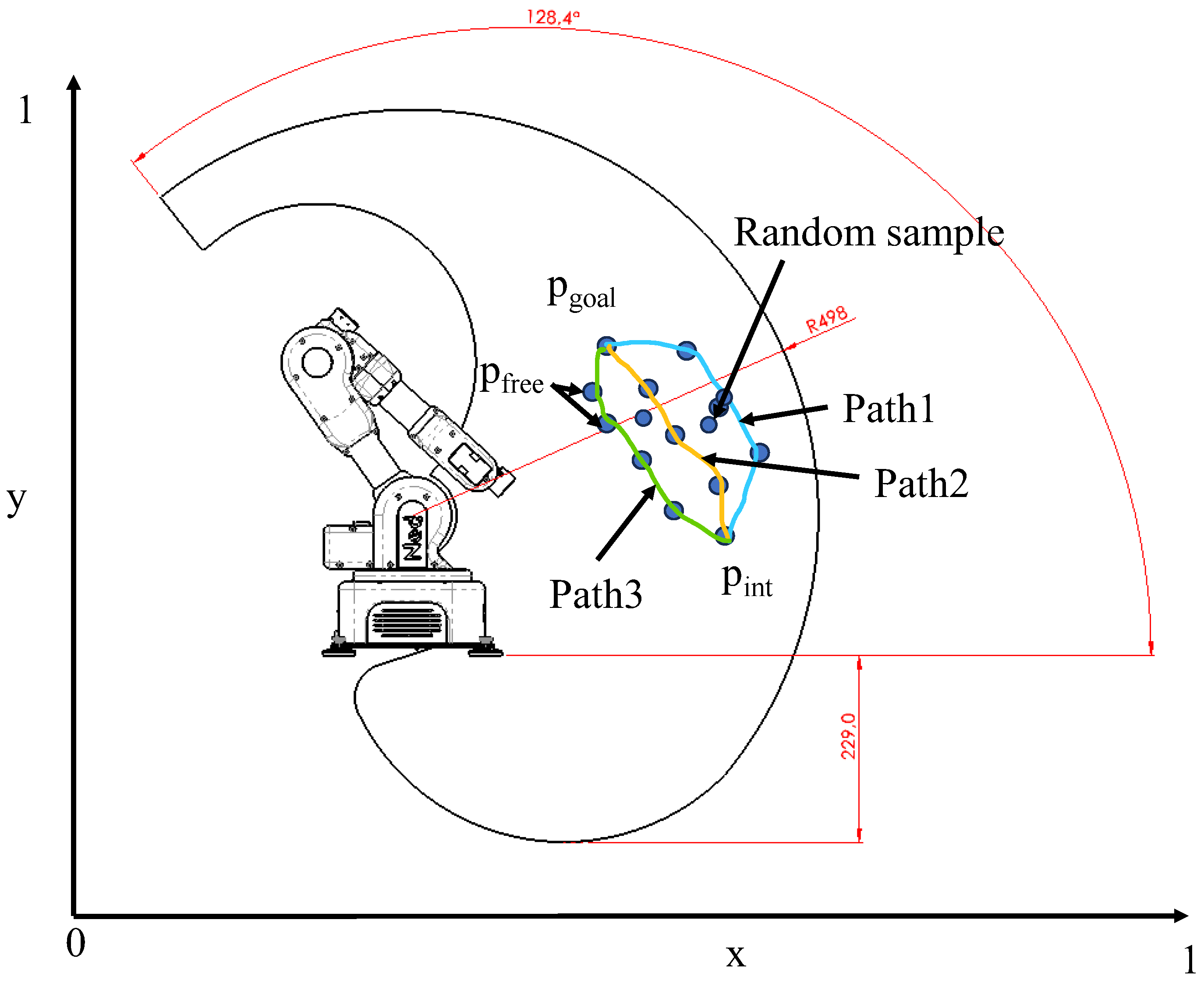
The feasible and optimal robot motion planning in the robot C-space can be formalized for C:[0, 1] in the robot C-space, where dimension, [x, y] ∈ , and, is the obstacle regions [16]. As depicted in Figure 2, if the start position () and goal position () are the elements of C-space free positions (), then the motion planning problem can be expressed as a function of [ , ]. For all the intermediate positions () for i = 1, 2, … n, where n is at the goal position, the total path trajectory function is .
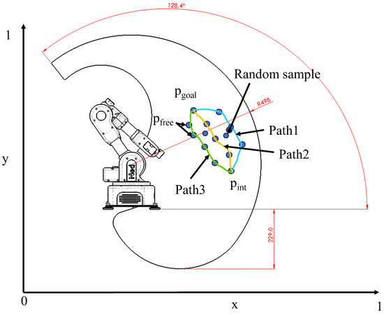
Figure 2.
Sampling-based path generation from an initial position () to goal position () in robot C-space.
The function in the bounded condition can generate a feasible and collision-free motion in the robot C-space.
3.3. Primitive Technique
3.3.1. Sampling
In the robot’s C-space (C), the sampling process, Sample: S ⊂ C is a map from the initial position to the sequences of position , such that the random variables for the sample, i ∈ N, where N is the set of the number of positions in the sampling process. The samples are considered independent, as well as identically distributed autonomously and identically distributed in the C-space.
Therefore, if there are collisions in the C-space, the robot motion in the robot free-space (), Sample can be defined as Samplefree : that returns the randomly distributed sequences for samples in Cfree. Therefore, in the entire robot workspace, it can be simplified as = ∩ Cfree.
3.3.2. Nearest Neighbor
In the sampling-based method, a graph can be denoted by G = (V, E), where vertex, V ⊂ C connects the edges (E) for the position . The nearest neighbor function for the V in terms of is expressed as (, )→ v ∈ V, for nearest vertices v [17,19]. The expression for the nearest neighbor can be written as
3.4. Description of Motion Planning Algorithms
3.4.1. Fundamental Rapidly Exploring Random Tree (RRT) Algorithm
The RRT algorithm [22] is designed primarily for single-query representations. In the most basic form, the algorithm incrementally generates a tree of feasible trajectories, embedded in the preliminary conditions. Algorithm 1 provides an overview of the basic RTT algorithm. The algorithm is started with a graph that has only one start position as its single vertex without any edges . After every iteration in the C-space, a position is sampled. An edge is set up to link up the nearest vertex v ∈ V in the random tree to the latest sample. If the connecting link is successful, is included in the set of vertices, and (, ) is then attached to the set of edges. The iteration in the original version of this algorithm is terminated as soon as the tree contains a node in the goal region.
| Algorithm 1: RRT Algorithm | |
| 1: | Define Tree in the robot workspace . |
| 2: | |
| 3: | for do |
| 4: | |
| 5: | [From Equation (1)] |
| 6: | |
| 7: | if collision-free then |
| 8: | , |
| 9: | end if |
| 10: | end for |
| 11: | return |
3.4.2. Rapidly Exploring Random Tree Star (RRT*) Algorithm
The RRT* algorithm [18,22] is an improved version of the basic RRT as defined in Section 3.4.1 that can deal with modeling errors caused by cycle formation by removing redundant edges that are not part of the shortest path from the tree’s initial position to a vertex. Algorithm 2 describes the RRT* algorithm.
| Algorithm 2: RRT* Algorithm | |
| 1: | Define Tree in the robot workspace |
| 2: | , |
| 3: | for do |
| 4: | |
| 5: | [From Equation (1)] |
| 6: | |
| 7: | if collision-free then |
| 8: | [From Equation (2)] |
| 9: | |
| 10: | |
| 11: | |
| 12: | |
| 13: | end if |
| 14: | end for |
| 15: | return |
The RRT* algorithm modifies the traditional RRT to avoid the formation of cycles by eliminating “redundant” edges, that is, edges that are not part of the shortest path from the root of the tree (i.e., the initial position) to a vertex. To satisfy this condition, there are two major inclusions for the RRT* algorithm: ChooseParent and Rewire including cost functions. The pseudocodes for both are described in Algorithms 3 and 4, respectively.
When is added to the tree, Algorithm 3 finds the parent node with the minimum cost-to-reach () value inside . It is to be noted that the computation of is related to the length of the path between the near node () and the newly generated node (). In a dynamic collision-free environment, cost function needs to be satisfied with the minimum cost to find the next parent node. The Rewire function in Algorithm 4 continues to connect the parent node to the nearest node in its C-space.
| Algorithm 3: | |
| 1: | |
| 2: | |
| 3: | for all do |
| 4: | |
| 5: | |
| 6: | if and collision-free then |
| 7: | |
| 8: | |
| 9: | end if |
| 10: | end for |
| 11: | return |
| Algorithm 4: | |
| 1: | for each do |
| 2: | |
| 3: | then |
| 4: | else if collision-free then |
| 5: | |
| 6: | |
| 7: | end if |
| 8: | end if |
| 9: | end for |
| 10: | return |
3.4.3. Flight Cost-Based RRT*
In this FC-RRT* algorithm, the maximum reach of the robot end-effector is determined as a cost function in terms of length (D) between two positions. As described in Section 3.3.1 for the sampling process, the length constraints can be calculated as
| Algorithm 5: FC-RRT* Algorithm | |
| 1: | Define Tree T, in the robot workspace W |
| 2: | , |
| 3: | for i = 1 to i = n do |
| 4: | |
| 5: | [From Equation (1)] |
| 6: | |
| 7: | [From Equation (2)] |
| 8: | for all do |
| 9: | rewire_ApplyRRT*() // For positive direction (Counterclockwise ro tation) |
| 10: | for all do |
| 11: | rewire_ApplyRRT*() // For negative direction (Clockwise rotation) |
| 12: | end for |
| 13: | end for |
| 14: | end for |
| 15: | return |
Equation (4) is used in FC-RRT* to estimate the flight cost function to stimulate new node extensions and to apply constraints to select new nodes. In this algorithm, the designed flight cost function is used for new node generations and to introduce flight constraints to screen new nodes. After obtaining the sample node (), the h_cost() function is applied to return the new node (). The heuristic information process guides new node extension. Algorithm 6 depicts the heuristic method for developing the new node extension. First, the Euclidean distances between each tree node and are computed individually. When the distance between the nodes is smaller than the highest segment distance () stipulated by FC-RRT* but greater than the minimum segment distance , is recognized as a potential new node. If the space goes beyond , the vertex formed by expanding in distance through in the path of to is determined as a possible new node. When the total flight cost of each path segment (between and ) is the shortest, the obtained trajectory is regarded to be the optimal path. Moreover, the rewire function is defined based on the joint rotation in both clockwise and counterclockwise directions.
| Algorithm 6: | |
| 1: | for all T. V do |
| 2: | if (Dmin ∥−∥≤ ) then |
| 3: | |
| 4: | then |
| 5: | |
| 6: | if collision-free then |
| 7: | h_cost [From Equation (4)] |
| 8: | end if |
| 9: | end for |
| 10: | return |
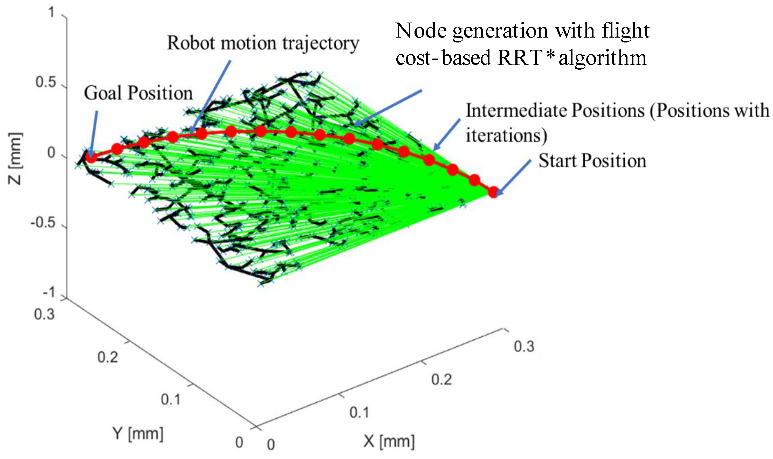
The parent node update strategy is followed by the Rewire function of FC-RRT*, as mentioned in Algorithm 5. Figure 3 depicts a robot motion trajectory generated by the FC-RRT* algorithm from a start position to a goal position, followed by the predefined intermediate positions. From the start to the goal position, each intermediate path () is generated using the FC-RRT* algorithm utilizing Algorithm 5. The expected intermediate points are first assumed based on the robot’s reference positions for setting command angles, as discussed in Section 4, whereas the black dots are the randomly generated nodes (). The red trajectory represents the position derived by using FC-RRT*.

Figure 3.
FC-RRT* algorithm is applied to generate robot motion trajectory.
3.4.4. Kinematic Approach to Robot Motion
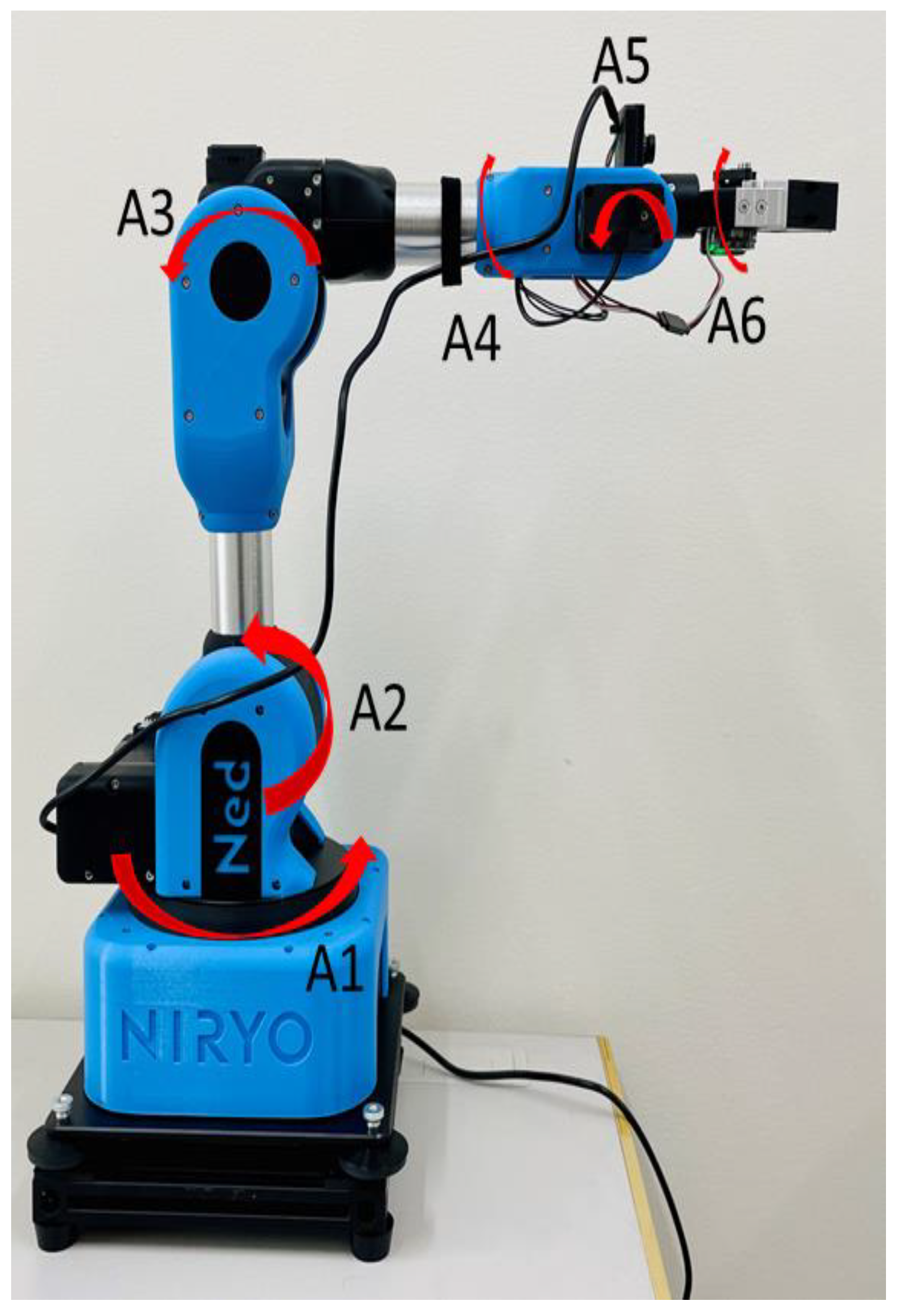
Kinematic solutions have proven to be extremely effective in determining the precise robot pose in 3D under dynamic settings [5,32,40]. Forward kinematics is the technique of determining end-effector position and velocity for goal-directed motion based on joint parameters. In this experiment, a 6DOF serial robot (as shown in Figure 4) is used for energy-efficient motion planning. The rotary axes of the robot are denoted as Aj, where j = 1, … 6 is the number of rotary joints for the six-axis robot.
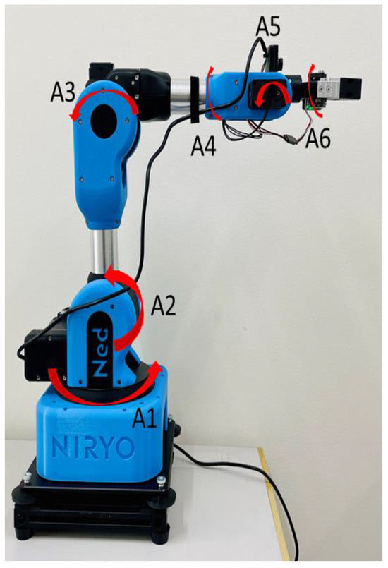
Figure 4.
Niryo Ned robot with 6DOF configuration.
The Denavit–Hartenberg [5,41] methodology is the most acceptable method for determining the homogeneous transformation matrix between the joint angles and the joint links that characterize the robot’s position and orientation. According to Equation (5), the four parameters that can be utilized to determine the robot’s position are joint angle , link twist , link length and link offset.
4. Methodology of the Experiments
The experiment is set up so that one axis rotates in the robot’s C-space while the other rotating axes remain fixed or at the zero angular position. In the literature, this type of experiment is referred to as the axis indexing test [9]. For example, when the A1 axis of the robot in Figure 1 rotates from t0 radians (rad) to 1 rad with an interval of supposing 0.1 rad while the A2-axis to A6-axis is kept at constant (0 rad), the experiment is defined as A1 axis indexing test. Table 1 shows the essential features of the robot in Figure 4.

Table 1.
Major features of Niryo NED robot *.
Figure 5 shows the example of the A1 axis indexing test in the Niryo Studio 1.8.8, which is a graphical human machine interface (HMI) and permits rapid and explicit control of Ned with an external workstation. In this situation, the A1 axis (joint 1 in Niryo studio) is rotated from 0 rad to 0.10 rad, while Joint 2 to Joint 6 are at the constant angular position at 0 rad.
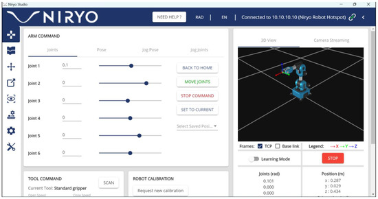
Figure 5.
Niryo Studio example while conducting A1 axis indexing test.
Table 2 shows the data for the A1 axis indexing test for the condition: θ1 = [0:0.1:1.5] rad, θ2 = θ3 = θ4= θ5 = θ6 = 0 rad, where θj is the angular position of the j axis.

Table 2.
Robot command pose for A1 axis indexing test for θ1 = [0 to 1.5] radian.
Similarly, for the other axes (A2 to A6), indexing tests are performed where the axis under experiment is rotated with the angular position, as shown in Table 3, while the other axes are kept constant at 0 rad.

Table 3.
Axis indexing test conditions for the A2 to A6 axes.
5. Experiment Results on Motion Planning and Energy Consumption
5.1. Motion Planning Results
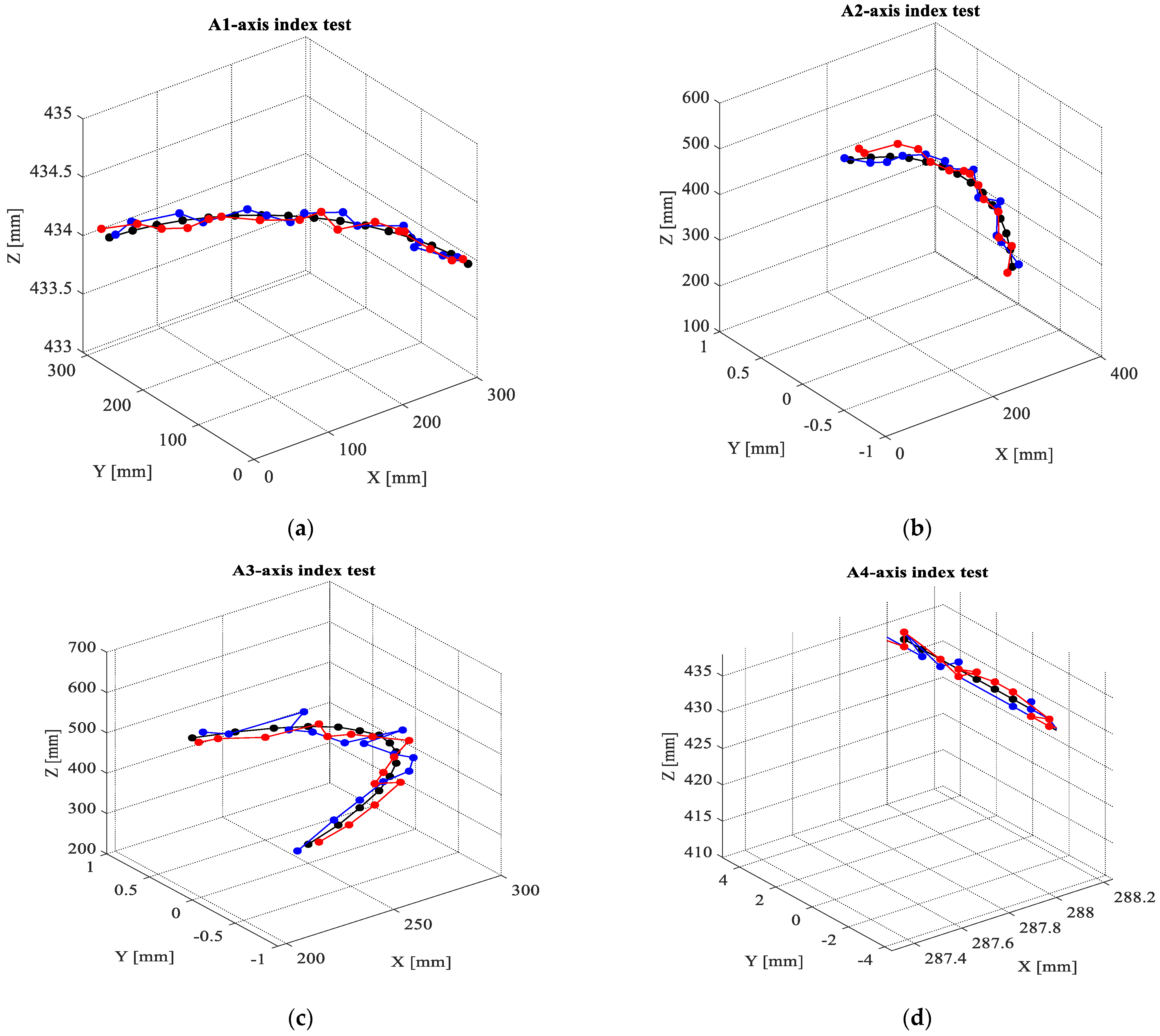
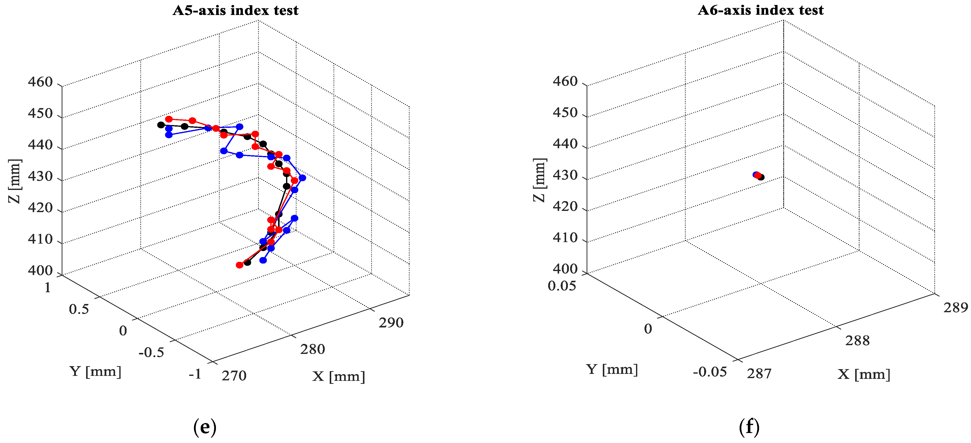
Figure 6 depicts the path trajectories for each AJ axis. The black paths are derived from the command angular position based on the Niryo Studio command positions stated in Section 4. The blue lines are from the kinematic solutions mentioned in Section 3.4.4, whereas the red paths are from the FC-RRT* algorithm discussed in Section 3.4.3. The command positions are the desired trajectory. When there is no deviation in the desired trajectory, the deviation in the XY plane should be zero.
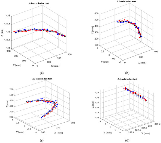
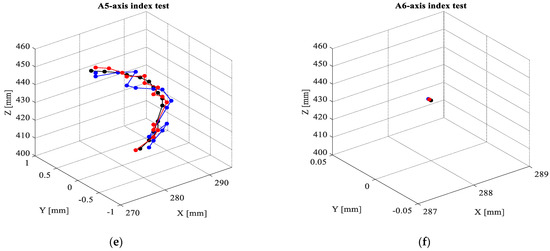
Figure 6.
Robot end-effector position in 3D during robot motion planning (a) A1 axis indexing test, (b) A2 axis indexing test, (c) A3 axis indexing test, (d) A4 axis indexing test, (e) A5 axis indexing test, and (f) A6 axis indexing test. The black pathways represent command positions, the blue paths represent solutions with kinematic parameters, and the red paths represent solutions with FC-RRT*.
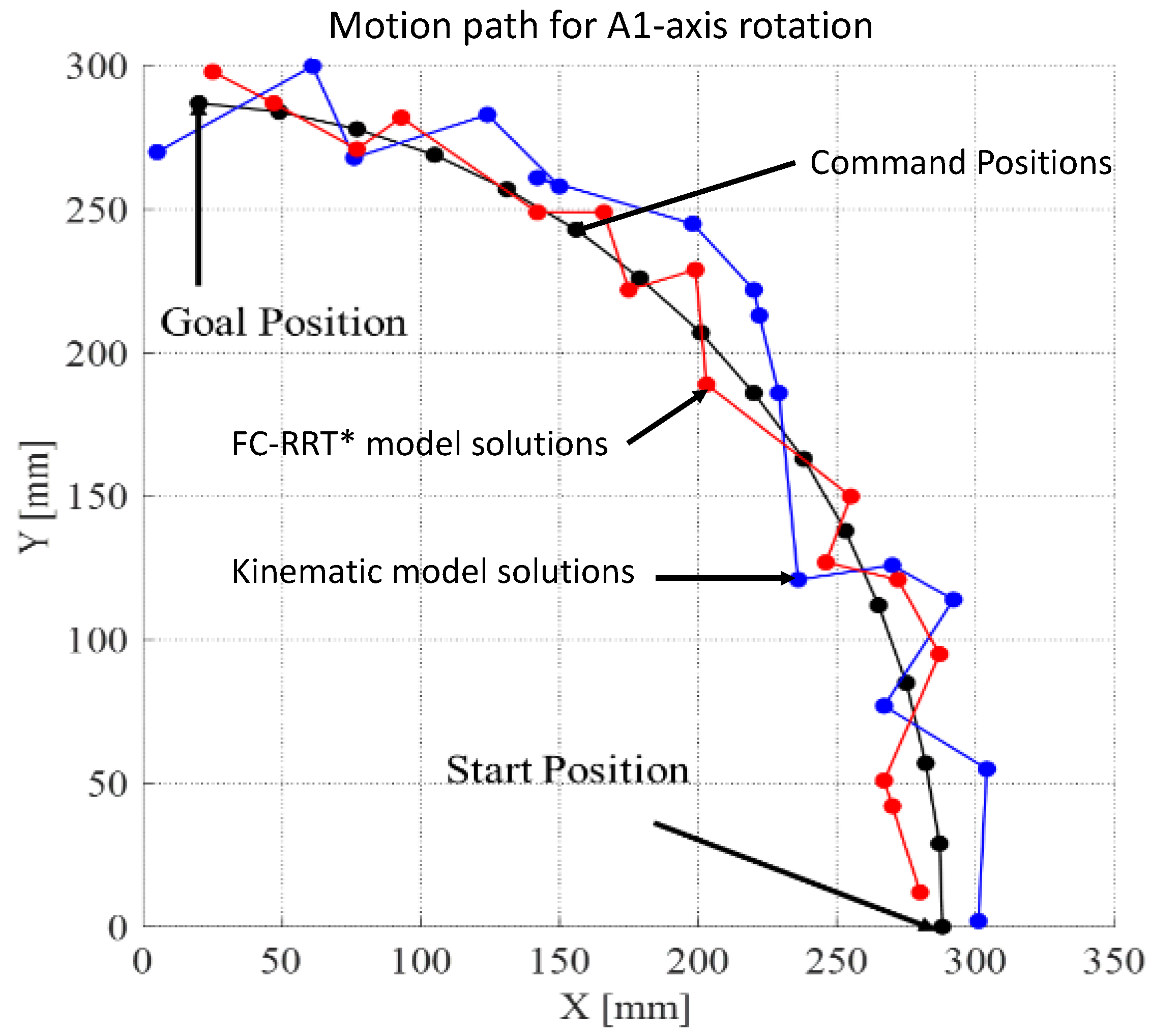
Figure 7 illustrates the deviation in the XY plane with the RRT* algorithm (green line), FC-RRT* algorithm (blue line), and kinematic solution (red line). The deviations are calculated as the difference between command positions (obtained from Niryo Studio) and the simulated position using the kinematic solution, RRT*, and FC-RRT* algorithms, respectively. The trajectories show a clear deviation in the XY plane. However, with the kinematic solution, the average deviation is 3 times larger than the solution with FC-RRT* because the FC-RRT* algorithm can minimize the traveling distance for the joint of the robot and optimize joint traveling time in the C-space simultaneously using the heuristic cost function.
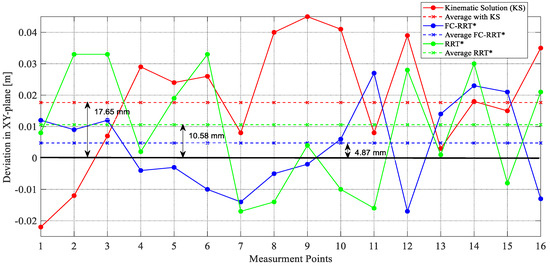
Figure 7.
Deviations in XY plane for the trajectories with RRT*, FC-RRT*, and kinematic solutions for A1 axis indexing test.
The measurements are performed following the A1 to A6 axis indexing tests as described in Section 5. When there is no deviation, the position of the vertical axis should be zero. The average deviations for the A1 to A6 axis indexing tests are shown in Table 4. The average deviation with the FC-RRT* algorithm is lower than with the kinematic solution and conventional RRT* algorithms, notably for the A1 to A3 axes.

Table 4.
The average deviation in the motion planning for A1 to A6 axes.
In robot C-space, Figure 8 shows the path trajectory in the XY plane (as an example, for the A1 axis indexing test).
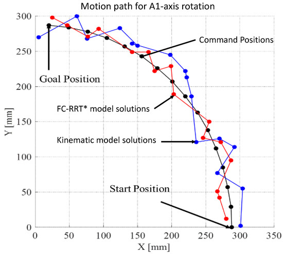
Figure 8.
A1 axis motion path in XY plane.
5.2. Energy Profile in Robot Motion
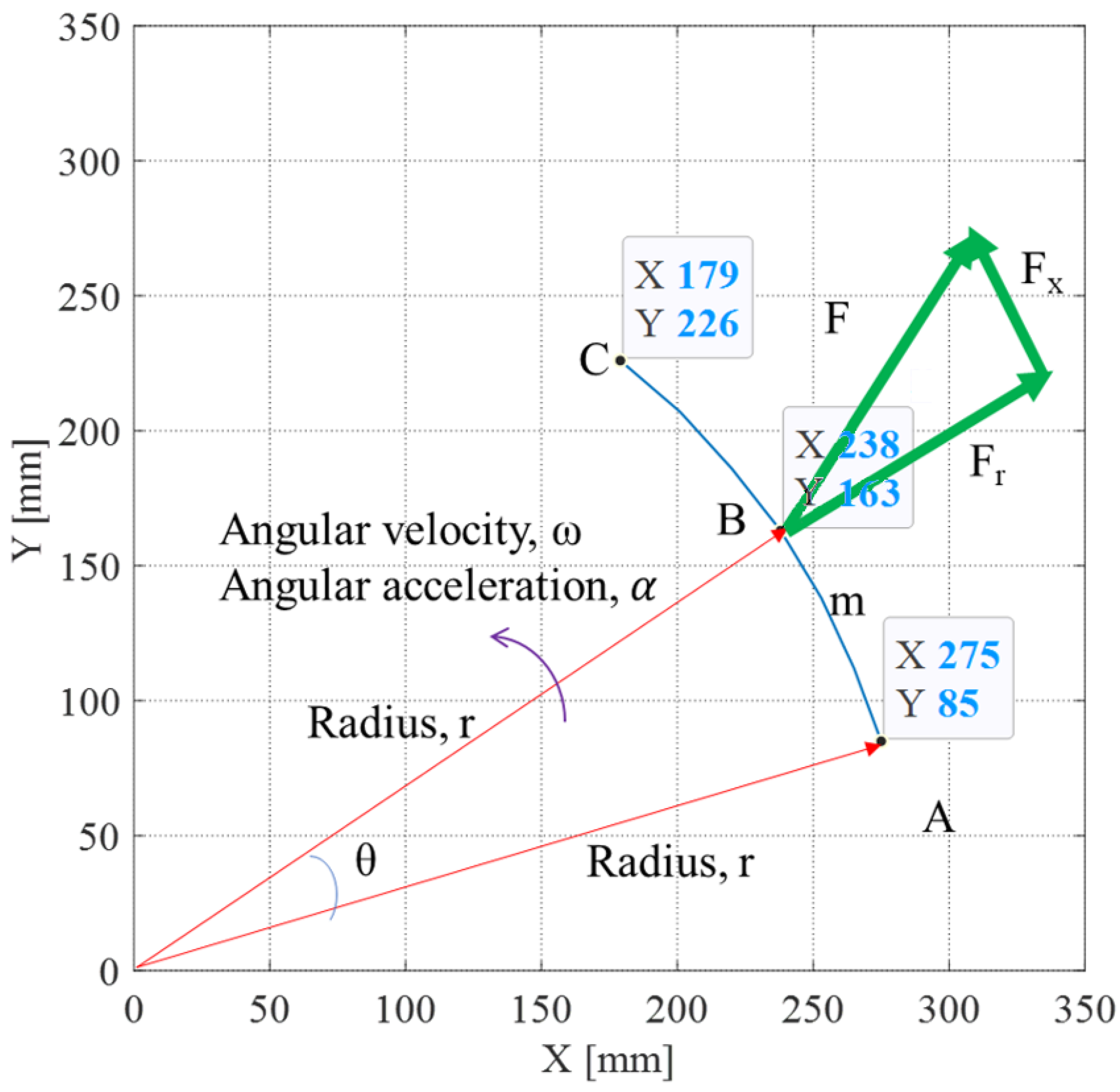
The energy profile of the robot motion is defined as the kinetic energy for rotating rigid bodies or, more precisely, work done on a rigid body rotating about a given axis [42,43]. Figure 9 depicts a rigid body rotating over an angle θi around a fixed axis (in this case the z-axis, which is perpendicular to the page if viewed on the XY plane) and passes through the origin, from position A (X, Y = 275, 85) through position B (X, Y = 238, 163) to position C (X, Y = 226, 179). For the position from A to B, the angular rotation (θ) is because of the effect of an exterior force F caused by the applied force (Fx) and tangential force (Fr) on position A. r is the radius of the circular motion trajectory, whereas, due to the external force F, the position A moves to position B with an angular velocity of change from ωA to ωB due to the change in angle from θA to θB and in time from tA to tB. The radius remains constant during the motion trajectory. When the robot’s end-effector position is known, the inverse kinematic solution may identify the joint angle parameters.

Figure 9.
Rigid body motion around a fixed axis.
Moreover, the circular motion of the robot is subjected to angular velocity and angular acceleration as a result of the robotic pick-and-place operation. Angular velocity (ω) can be defined as the change in angular position as a function of time. The motion’s angular velocity can be defined as
Angular acceleration () of the robot’s circular motion is defined as the rate of change in angular velocity with change in time. Therefore, it can be expressed as
As illustrated in Figure 9, there is a displacement (m) around the rotational angle (θ) with a fixed radius (r) due to the external force (F). Therefore, it can be written in vector form as
When r is fixed, Equation (8) can be modified to account for the infinitesimal change in displacement as
Considering the work–energy theorem for rotational motion and using the definition of work, the work (Wrobot) can be obtained as
However, the acting torque (τ) on the circular motion of the rigid body can be expressed in relation to the acting force (F) and the radius (r) as
Therefore, the torque triggered by the acting force on the robot’s rigid body motion causes the rotational work in the robot motion as
Considering Figure 9, the rotational work that causes position A to move to position B can be expressed as
Instantaneous power can be defined as the rate of accomplishing work using the above formulae.
The energy consumption formulation is based on circular motion. Therefore, to comply with the indexing test, only the circular motion is considered. Note that, with this type of motion, the effect of one axis on another axis can also be determined in an industrial manipulator [41].
6. Discussion on Energy Consumption
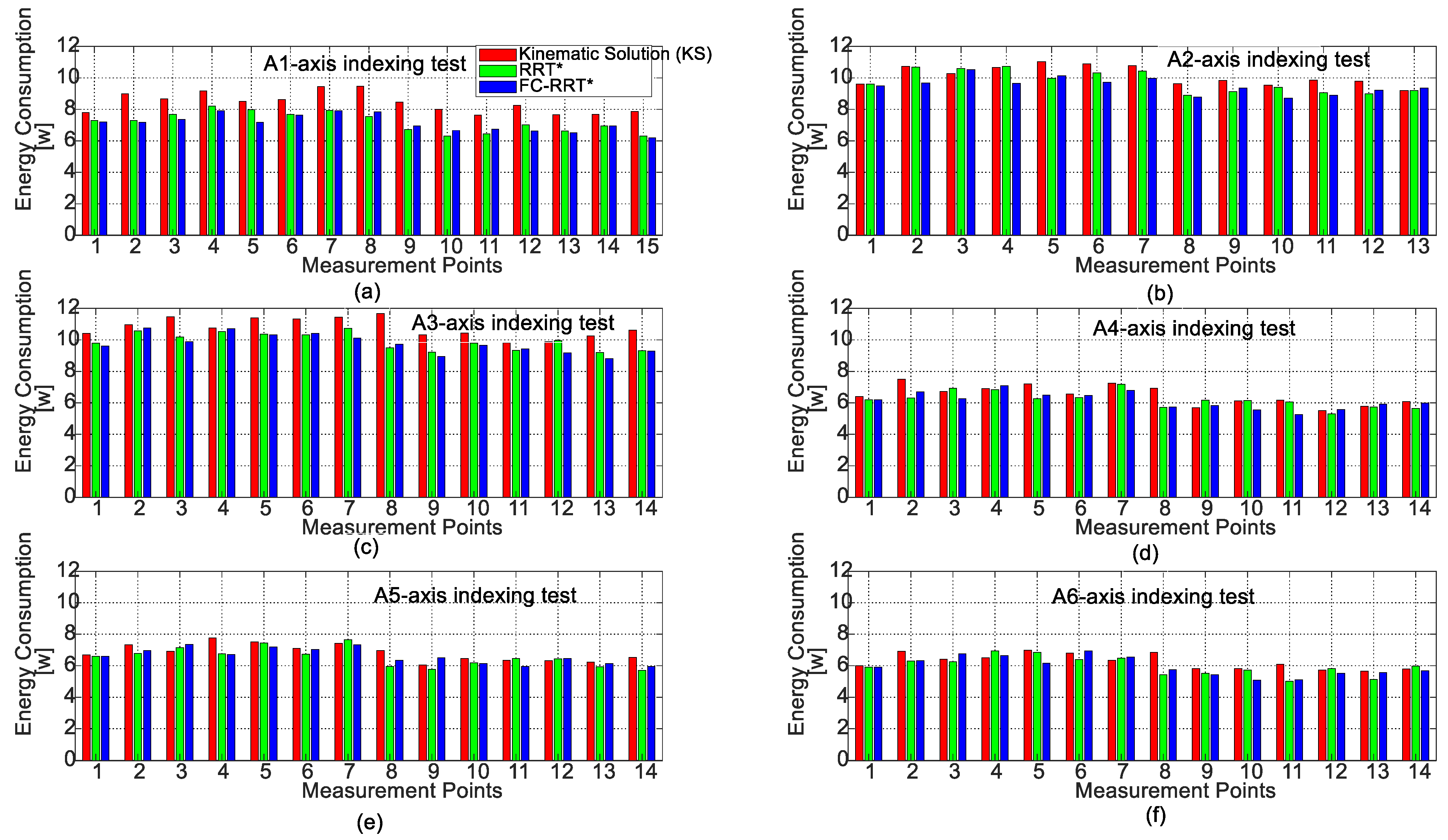
The energy consumption of an industrial robot with a 6DOF configuration in robotic pick-and-place operation is investigated in this study. Figure 10 represents the power consumption of the robot for the A1 to A6 axis indexing test using the work–energy hypothesis for circular path trajectory. The bar graphs show the calculated energy consumption or variation in the corresponding energy consumption for all the measurement points, using kinematic solutions as well as applying conventional RRT* and the novel FC-RRT* algorithm. Table 5 displays the average power consumption results as well as the changes in efficiency for all axes. The torque curves are not represented because the torque curve is the motor’s torque output at different speeds or operating points. In our experiment, the rotational speed is fixed and controlled by the robot controller. Moreover, the torque is determined as a function of the displacement of rotary joint angles and the rotational distance, applying the work–energy theorem as detailed in Section 5.2. The results in Table 5 show a significant improvement (more than 10%) in power consumption for the A1 to A3 axis by applying the FC-RRT* algorithm to the kinematic solution. However, the power consumption for the A4 to A6 axes is less than 5%. The convergence rate of FC-RRT* is faster than that of the kinematic solution because the heuristic cost function is defined as a function of the minimal distance (as in Equation (4)) in the robot C-space, providing an energy-efficient solution for the 6DOF serial robot.

Figure 10.
Energy consumption for A1 to A6 axis indexing test. (a) A1 axis indexing test, (b) A2 axis indexing test, (c) A3 axis indexing test, (d) A4 axis indexing test, (e) A5 axis indexing test, and (f) A6 axis indexing test.

Table 5.
Average power consumption for A1 to A6 axis applying kinematic solution, conventional RRT*, and novel FC-RRT* algorithm.
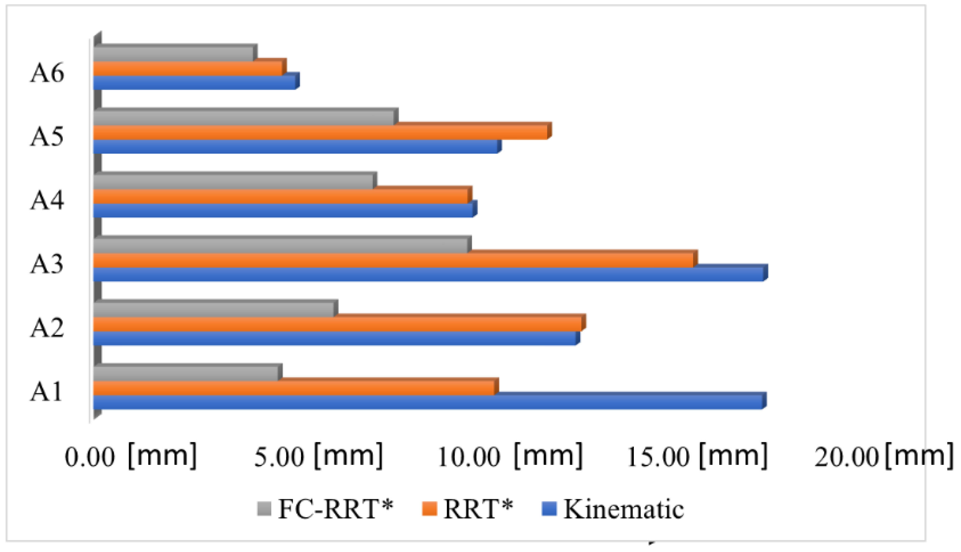
While addressing energy consumption, the study also focuses on robot motion planning optimization using graph search-based motion planning algorithms. To optimize the motion trajectory, this study employs a novel sampling-based method known as the flight cost-based RRT* (FC-RRT*). The variance in position with the FC-RRT* method is much better than the kinematic solution and the RRT* algorithm, as shown in Figure 11. However, in some circumstances, the divergence using the conventional RRT* approach is poorer (A2 and A5 axis) than the kinematic solution. Conventional RRT* generates new nodes in the C-space in random order, whereas FC-RRT* generates new nodes in a specified direction (shown in Algorithm 5—steps 9 and 11) with the minimal heuristic cost function, which improves the positioning deviation solutions for FC-RRT*. On the other hand, for a 6DOF serial robot, the A1 to A3 axes have the highest influence on the robot’s pose since they span most of the workspace. Therefore, the positioning deviation improvements by using FC-RRT* for the A1 to A3 axes are greater than for the other axes, which is also probably attributable to higher energy consumption for the A1 to A3 axes (shown in Table 5). A balance of energy consumption and total motion time should be considered when applying the FC-RRT* method. Setting an appropriate weighting factor for the flight cost and the parameter of should be carefully considered.

Figure 11.
Deviation from the desired position in motion planning.
There are several case studies that can be applied to the proposed approach to complex pick-and-place environments where efficiently avoiding collisions while optimizing for energy efficiency is important. The proposed algorithm can find collision avoidance motion and trajectory planning efficiently while reducing energy consumption. These case studies will be conducted in our future study.
7. Conclusions
This research proposes an energy-efficient industrial robotics motion planning strategy using the FC-RRT* method to generate nodes in a predetermined direction and then calculate energy consumption using the circle point method. After optimizing the motion trajectory, power consumption is computed using the work–energy hypothesis for a rotational motion of a rigid body. The FC-RRT* method consumes up to 16.5% less energy than the robot kinematic technique. This study is a step toward energy optimization in industrial robot motion planning. The FC-RRT* strategy in motion planning enables the node generation in a predetermined direction rather than a random approach, and then the circle point method is used to determine the energy consumption of the robot, which is a novel addition to this study. In this study, after optimizing the motion trajectory, the power consumption is computed using the work–energy hypothesis for a rotational motion of a rigid body, for which the axis indexing test is essential. The results show that for the A1 axis indexing test, the FC-RRT* method utilizes a maximum of 16.5% less energy than the conventional kinematic technique. However, only the robot’s circular motion is studied in this experiment, and all other types of motion trajectories are ignored. Additionally, the impact of dynamic elements such as payload change, friction impact, and gravity are not considered when defining energy-efficient motion planning. Another shortcoming of this study is that the experiment is carried out at 20% of the rated speed for all rotating axes. The limitations of the current study will be addressed in our future investigation. An exhaustive comparison with conventional methods will be the future work. Moreover, experiments conducted were based on robotic indexing tests, which are fundamental to a robot’s performance. However, we need to test various other performance aspects, such as dynamic contour error (ISO 230-4 [44]), thermal error (ISO 230-3 [44]), and vibration (ISO 230-8 [44]) in our future works.
Author Contributions
Conceptualization, M.M.A., T.N., Z.L. and T.F.; methodology, M.M.A.; software, M.M.A.; validation, M.M.A., T.N., Z.L. and T.F.; formal analysis, M.M.A.; investigation, M.M.A., T.N., Z.L. and T.F.; resources, M.M.A. and T.N., data curation, M.M.A.; writing—original draft preparation, M.M.A.; writing—review and editing, M.M.A., T.N., Z.L. and T.F.; visualization, M.M.A.; supervision, T.N.; project administration, T.N.; funding acquisition, T.N. All authors have read and agreed to the published version of the manuscript.
Funding
This research is subsidized by the New Energy and Industrial Technology Development Organization (NEDO) under project JPNP20016.
Data Availability Statement
The data that support the findings of this study are available on request from the corresponding author, Md Moktadir Alam.
Acknowledgments
This paper is one of the achievements of joint research with and is jointly owned copyrighted material of ROBOT Industrial Basic Technology Collaborative Innovation Partnership.
Conflicts of Interest
The authors declare no conflict of interest.
Abbreviations
| RRT | Rapidly exploring random tree |
| RRT* | Rapidly exploring random tree star |
| 6DOF | Six degree of freedom |
| FC-RRT | Flight cost-based rapidly exploring random tree star |
| C-space | Configuration space |
| PRM | Probabilistic roadmap |
| P-PRM | Potential field-based probabilistic roadmap |
| MOD-RRT* | Multi-objective dynamic rapidly exploring random tree star |
| UAV | Unmanned aerial vehicles |
| HMI | Human machine interface |
| KS | Kinematic solution |
Nomenclature
| Sets | |
| The set of the number of positions in the sampling process | |
| C-space | |
| Robot free space | |
| Set of vertices, | |
| Set of edges | |
| Set of free positions | |
| Indexes | |
| Index for position | |
| The number of rotary joints for the six-axis robot | |
| Parameters | |
| Robot workspace | |
| Obstacle region | |
| Start position | |
| Goal position | |
| Radius | |
| Variables | |
| Intermediate position of | |
| (, , ) | 3D end-effector position of |
| Nearest vertex, | |
| A sampled position, | |
| A tree which is a pair of | |
| The nearest position generated by Equation (1) | |
| A near position generated by Equation (2) | |
| A new position generated by and | |
| Length between two positions | |
| Cost between two points | |
| The minimum path lengths between the optional path segments | |
| The maximum path lengths between the optional path segments | |
| Kinematic | |
| The rotary axes of a robot | |
| Joint angle of joint | |
| Link twist of joint | |
| Link length of joint | |
| Link offset of joint | |
| The transformation matrix between the joints | |
| Energy profile | |
| Angular velocity | |
| Angular acceleration | |
| Displacement | |
| External force | |
| Work of robot | |
| Acting torque | |
| The rotational work that causes position to move to position |
References
- Gasparetto, A.; Boscariol, P.; Lanzutti, A.; Vidoni, R. Path Planning and Trajectory Planning Algorithms: A General Overview. In Motion and Operation Planning of Robotic Systems; Carbone, G., Gomez-Bravo, F., Eds.; Mechanisms and Machine Science; Springer International Publishing: Cham, Switzerland, 2015; Volume 29, pp. 3–27. ISBN 978-3-319-14704-8. [Google Scholar]
- Wang, J.; Zhang, T.; Ma, N.; Li, Z.; Ma, H.; Meng, F.; Meng, M.Q.-H. A survey of Learning-Based Robot Motion Planning. IET Cyber-Syst. Robot. 2021, 3, 302–314. [Google Scholar] [CrossRef]
- Zhou, C.; Huang, B.; Fränti, P. A Review of Motion Planning Algorithms for Intelligent Robots. J. Intell. Manuf. 2022, 33, 387–424. [Google Scholar] [CrossRef]
- Sánchez-Ibáñez, J.R.; Pérez-Del-Pulgar, C.J.; García-Cerezo, A. Path Planning for Autonomous Mobile Robots: A Review. Sensors 2021, 21, 7898. [Google Scholar] [CrossRef]
- Ibaraki, S.; Theissen, N.A.; Archenti, A.; Alam, M. Evaluation of Kinematic and Compliance Calibration of Serial Articulated Industrial Manipulators. Int. J. Autom. Technol. 2021, 15, 567–580. [Google Scholar] [CrossRef]
- Chettibi, T.; Lemoine, P. Generation of Point to Point Trajectories for Robotic Manipulators under Electro-Mechanical Constraints. Int. Rev. Mech. Eng. 2007, 1, 131–143. [Google Scholar]
- Salzman, O. Sampling-Based Robot Motion Planning. Commun. ACM 2019, 62, 54–63. [Google Scholar] [CrossRef]
- Ibaraki, S.; Fukuda, K.; Alam, M.M.; Morita, S.; Usuki, H.; Otsuki, N.; Yoshioka, H. Novel Six-Axis Robot Kinematic Model with Axis-to-Axis Crosstalk. CIRP Ann. 2021, 70, 411–414. [Google Scholar] [CrossRef]
- Alam, M.; Ibaraki, S.; Fukuda, K.; Morita, S.; Usuki, H.; Otsuki, N.; Yoshioka, H. Inclusion of Bidirectional Angular Positioning Deviations in the Kinematic Model of a Six-DOF Articulated Robot for Static Volumetric Error Compensation. IEEE/ASME Trans. Mechatronics 2022, 27, 4339–4349. [Google Scholar] [CrossRef]
- Kang, T.-W.; Kang, J.-G.; Jung, J.-W. A Bidirectional Interpolation Method for Post-Processing in Sampling-Based Robot Path Planning. Sensors 2021, 21, 7425. [Google Scholar] [CrossRef]
- Kavraki, L.; Svestka, P.; Latombe, J.-C.; Overmars, M. Probabilistic Roadmaps for Path Planning in High-Dimensional Configuration Spaces. IEEE Trans. Robot. Autom. 1996, 12, 566–580. [Google Scholar] [CrossRef]
- Geraerts, R.; Overmars, M.H. A Comparative Study of Probabilistic Roadmap Planners. In Algorithmic Foundations of Robotics V; Boissonnat, J.-D., Burdick, J., Goldberg, K., Hutchinson, S., Eds.; Springer Tracts in Advanced Robotics; Springer: Berlin/Heidelberg, Germany, 2004; Volume 7, pp. 43–57. ISBN 978-3-642-07341-0. [Google Scholar]
- Sun, Y.; Gao, B. Improvement of the Probabilistic Roadmap Planner Algorithm for Mobile Robots. In Proceedings of the 2021 4th International Conference on Algorithms, Computing and Artificial Intelligence, ACM, Sanya, China, 22 December 2021; pp. 1–6. [Google Scholar]
- Alarabi, S.; Luo, C.; Santora, M. A PRM Approach to Path Planning with Obstacle Avoidance of an Autonomous Robot. In Proceedings of the 2022 8th International Conference on Automation, Robotics and Applications (ICARA), Prague, Czech, 18 February 2022; pp. 76–80. [Google Scholar]
- Kaltsoukalas, K.; Makris, S.; Chryssolouris, G. On Generating the Motion of Industrial Robot Manipulators. Robot. Comput.-Integr. Manuf. 2015, 32, 65–71. [Google Scholar] [CrossRef]
- Karaman, S.; Frazzoli, E. Sampling-Based Algorithms for Optimal Motion Planning. arXiv 2011, arXiv:1105.1186. [Google Scholar]
- Karaman, S.; Walter, M.R.; Perez, A.; Frazzoli, E.; Teller, S. Anytime Motion Planning Using the RRT*. In Proceedings of the 2011 IEEE International Conference on Robotics and Automation, Shanghai, China, 9–13 May 2011; pp. 1478–1483. [Google Scholar]
- LaValle, S.M.; Kuffner, J.J. Randomized Kinodynamic Planning. Int. J. Robot. Res. 2001, 20, 378–400. [Google Scholar] [CrossRef]
- Chen, J.; Zhou, Y.; Gong, J.; Deng, Y. An Improved Probabilistic Roadmap Algorithm with Potential Field Function for Path Planning of Quadrotor. In Proceedings of the 2019 Chinese Control Conference (CCC), Guangzhou, China, 27–30 July 2019; pp. 3248–3253. [Google Scholar]
- Wang, Z.; Tian, G. Hybrid Offline and Online Task Planning for Service Robot Using Object-Level Semantic Map and Probabilistic Inference. Inf. Sci. 2022, 593, 78–98. [Google Scholar] [CrossRef]
- Noreen, I.; Khan, A.; Habib, Z. A Comparison of RRT, RRT* and RRT*-Smart Path Planning Algorithms. Available online: https://www.semanticscholar.org/paper/A-Comparison-of-RRT%2C-RRT*-and-RRT*-Smart-Path-Noreen-Khan/a06c3e978e3cb8da7f94079745142520ca930796 (accessed on 1 June 2022).
- Qi, J.; Yang, H.; Sun, H. MOD-RRT*: A Sampling-Based Algorithm for Robot Path Planning in Dynamic Environment. IEEE Trans. Ind. Electron. 2021, 68, 7244–7251. [Google Scholar] [CrossRef]
- Kwon, H.; Cha, D.; Seong, J.; Lee, J.; Chung, W. Trajectory Planner CDT-RRT* for Car-Like Mobile Robots toward Narrow and Cluttered Environments. Sensors 2021, 21, 4828. [Google Scholar] [CrossRef]
- Fang, T.; Ding, Y. A Sampling-Based Motion Planning Method for Active Visual Measurement with an Industrial Robot. Robot. Comput.-Integr. Manuf. 2022, 76, 102322. [Google Scholar] [CrossRef]
- Zhang, S.; Xia, Q.; Chen, M.; Cheng, S. Multi-Objective Optimal Trajectory Planning for Robotic Arms Using Deep Reinforcement Learning. Sensors 2023, 23, 5974. [Google Scholar] [CrossRef]
- Fevgas, G.; Lagkas, T.; Argyriou, V.; Sarigiannidis, P. Coverage Path Planning Methods Focusing on Energy Efficient and Cooperative Strategies for Unmanned Aerial Vehicles. Sensors 2022, 22, 1235. [Google Scholar] [CrossRef] [PubMed]
- Liu, S.; Sun, D. Optimal Motion Planning of a Mobile Robot with Minimum Energy Consumption. In Proceedings of the 2011 IEEE/ASME International Conference on Advanced Intelligent Mechatronics (AIM), Budapest, Hungary, 3–7 July 2011; pp. 43–48. [Google Scholar]
- Zhang, H.; Zhang, Y.; Yang, T. A Survey of Energy-Efficient Motion Planning for Wheeled Mobile Robots. Ind. Robot. Int. J. Robot. Res. Appl. 2020, 47, 607–621. [Google Scholar] [CrossRef]
- Plooij, M.; Wisse, M.; Vallery, H. Reducing the Energy Consumption of Robots Using the Bidirectional Clutched Parallel Elastic Actuator. IEEE Trans. Robot. 2016, 32, 1512–1523. [Google Scholar] [CrossRef]
- Liu, A.; Liu, H.; Yao, B.; Xu, W.; Yang, M. Energy Consumption Modeling of Industrial Robot Based on Simulated Power Data and Parameter Identification. Adv. Mech. Eng. 2018, 10, 168781401877385. [Google Scholar] [CrossRef]
- Nonoyama, K.; Liu, Z.; Fujiwara, T.; Alam, M.; Nishi, T. Energy-Efficient Robot Configuration and Motion Planning Using Genetic Algorithm and Particle Swarm Optimization. Energies 2022, 15, 2074. [Google Scholar] [CrossRef]
- Hovgard, M.; Lennartson, B.; Bengtsson, K. Applied Energy Optimization of Multi-Robot Systems through Motion Parameter Tuning. CIRP J. Manuf. Sci. Technol. 2021, 35, 422–430. [Google Scholar] [CrossRef]
- Pellegrinelli, S.; Borgia, S.; Pedrocchi, N.; Villagrossi, E.; Bianchi, G.; Tosatti, L.M. Minimization of the Energy Consumption in Motion Planning for Single-robot Tasks. Procedia CIRP 2015, 29, 354–359. [Google Scholar] [CrossRef]
- Carabin, G.; Scalera, L. On the Trajectory Planning for Energy Efficiency in Industrial Robotic Systems. Robotics 2020, 9, 89. [Google Scholar] [CrossRef]
- Pellicciari, M.; Berselli, G.; Leali, F.; Vergnano, A. A Method for Reducing the Energy Consumption of Pick-and-Place Industrial Robots. Mechatronics 2013, 23, 326–334. [Google Scholar] [CrossRef]
- Pastras, G.; Fysikopoulos, A.; Chryssolouris, G. A Theoretical Investigation on the Potential Energy Savings by Optimization of the Robotic Motion Profiles. Robot. Comput.-Integr. Manuf. 2019, 58, 55–68. [Google Scholar] [CrossRef]
- Feng, Y.; Ji, Z.; Gao, Y.; Zheng, H.; Tan, J. An Energy-Saving Optimization Method for Cyclic Pick-and-Place Tasks Based on Flexible Joint Configurations. Robot. Comput.-Integr. Manuf. 2021, 67, 102037. [Google Scholar] [CrossRef]
- Pan, Y.; Al-Hadithi, B.M.; Yang, C. Editorial: AI for Robot Modeling, Path Planning, and Intelligent Control. Front. Robot. AI 2020, 7, 19. [Google Scholar] [CrossRef]
- Guo, Y.; Liu, X.; Liu, X.; Yang, Y.; Zhang, W. FC-RRT*: An Improved Path Planning Algorithm for UAV in 3D Complex Environment. ISPRS Int. J. Geo-Inform. 2022, 11, 112. [Google Scholar] [CrossRef]
- Alam, M.M.; Ibaraki, S.; Fukuda, K. Kinematic Modeling of Six-Axis Industrial Robot and Its Parameter Identification: A Tutorial. Int. J. Autom. Technol. 2021, 15, 599–610. [Google Scholar] [CrossRef]
- Messay, T.; Ordóñez, R.; Marcil, E. Computationally Efficient and Robust Kinematic Calibration Methodologies and Their Application to Industrial Robots. Robot. Comput.-Integr. Manuf. 2016, 37, 33–48. [Google Scholar] [CrossRef]
- Alyushin, Y.A. Calculation of the Kinetic Energy of a Rigid Body in the General Case of Three-Dimensional Motion with Arbitrary Rotation. J. Mach. Manuf. Reliab. 2022, 51, 9–19. [Google Scholar] [CrossRef]
- Kang, H.; Liu, C.; Jia, Y.-B. Inverse Dynamics and Energy Optimal Trajectories for a Wheeled Mobile Robot. Int. J. Mech. Sci. 2017, 134, 576–588. [Google Scholar] [CrossRef]
- ISO Standards. Available online: https://www.iso.org/standards.html (accessed on 1 January 2023).
Disclaimer/Publisher’s Note: The statements, opinions and data contained in all publications are solely those of the individual author(s) and contributor(s) and not of MDPI and/or the editor(s). MDPI and/or the editor(s) disclaim responsibility for any injury to people or property resulting from any ideas, methods, instructions or products referred to in the content. |
© 2023 by the authors. Licensee MDPI, Basel, Switzerland. This article is an open access article distributed under the terms and conditions of the Creative Commons Attribution (CC BY) license (https://creativecommons.org/licenses/by/4.0/).

