

Prediction Modeling of Flue Gas Control for Combustion Efficiency Optimization for Steel Mill Power Plant Boilers Based on Partial Least Squares Regression (PLSR)


Abstract
:1. Introduction
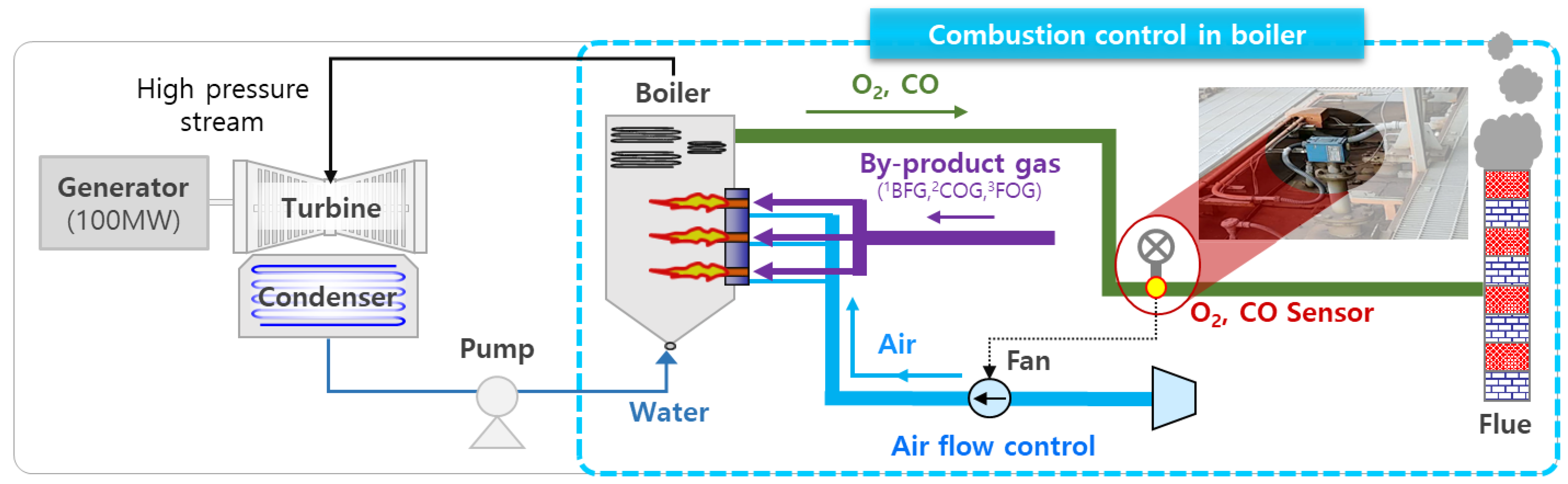
1.1. Background of Study
1.2. Problem Statement and Objectives
1.3. Literature Review
1.3.1. Conventional Studies on Improvements in Power Plant Efficiency
1.3.2. Studies on Boiler Flue Gas Prediction
1.3.3. Boiler Combustion Efficiency Improvement Using AI
1.3.4. Limitations of Previous Research
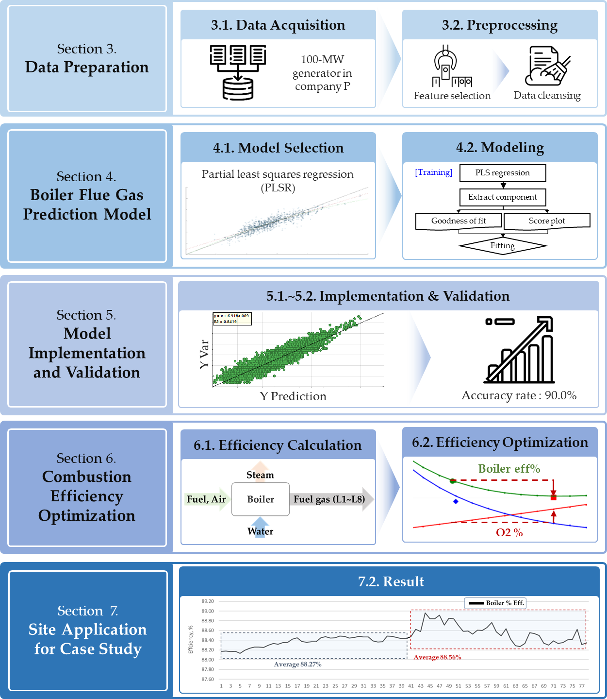
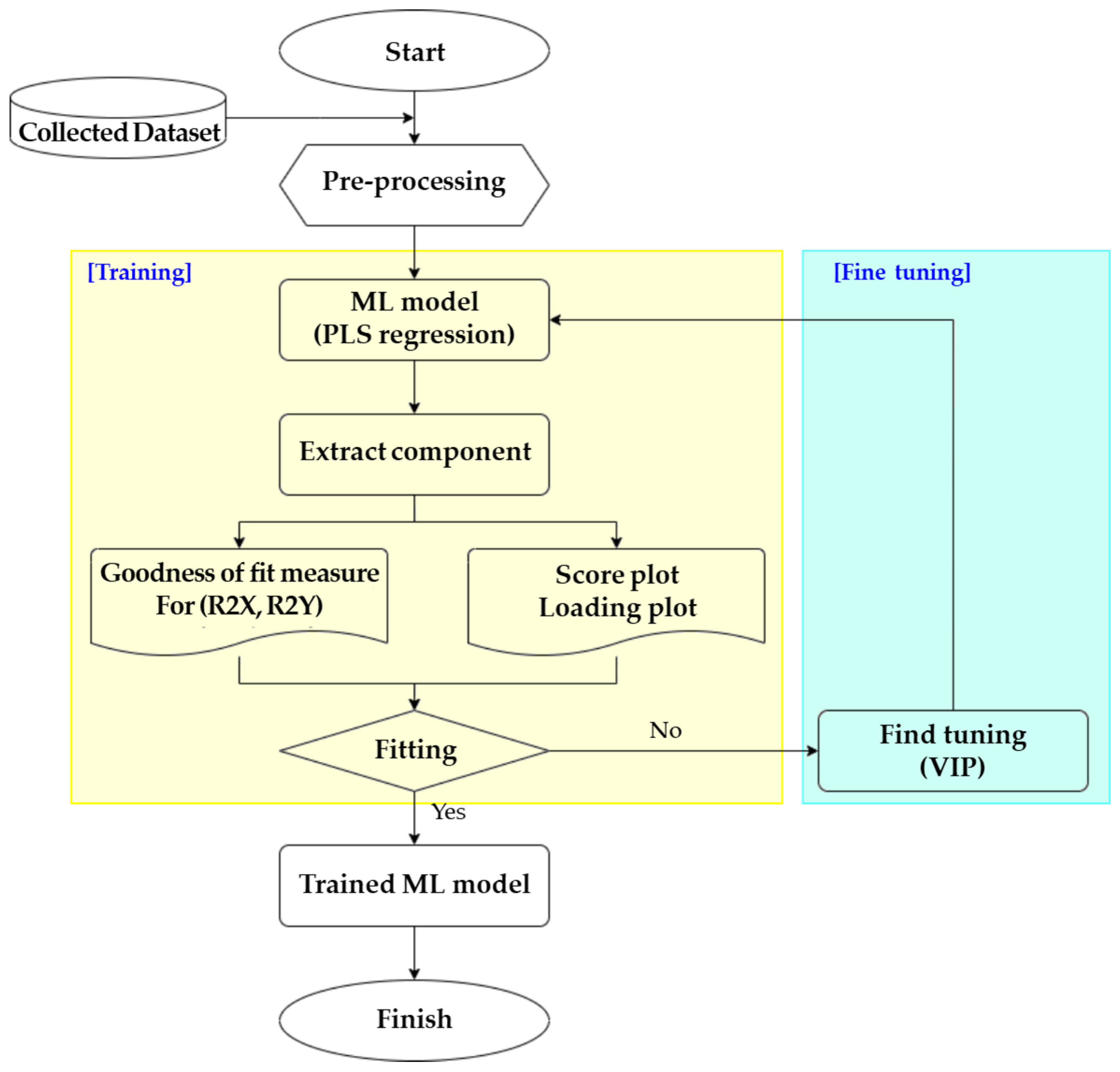
2. Research Process
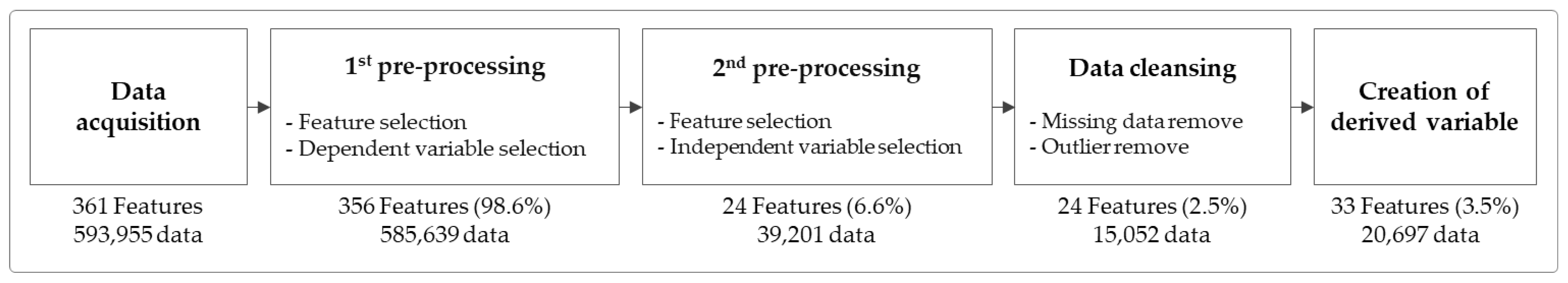
3. Data Preparation
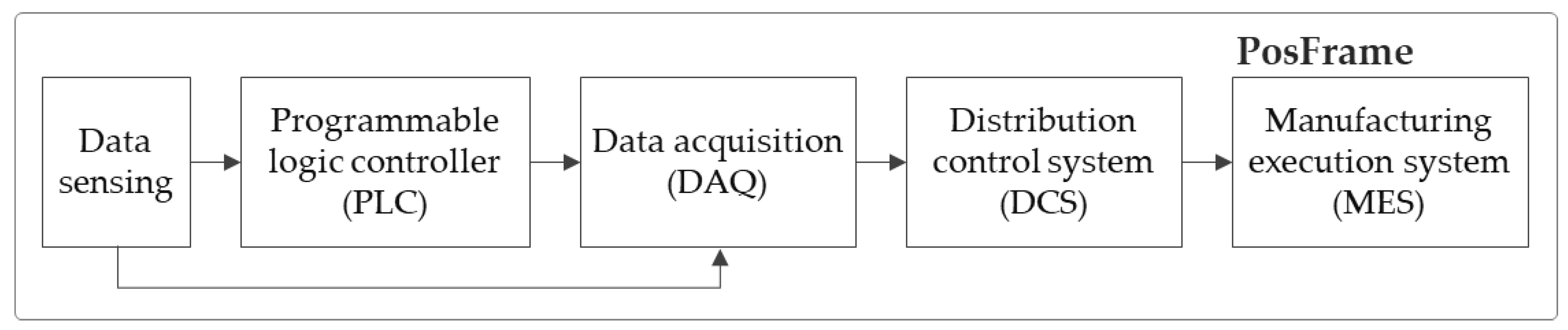
3.1. Data Acquisition
3.2. Data Preprocessing
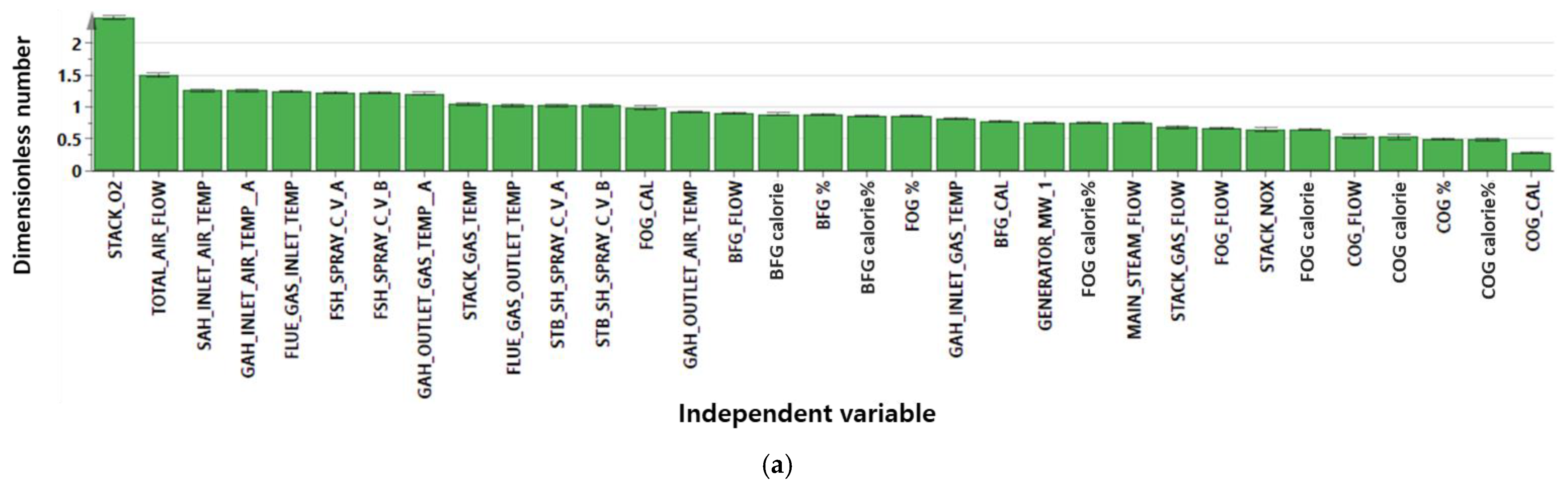
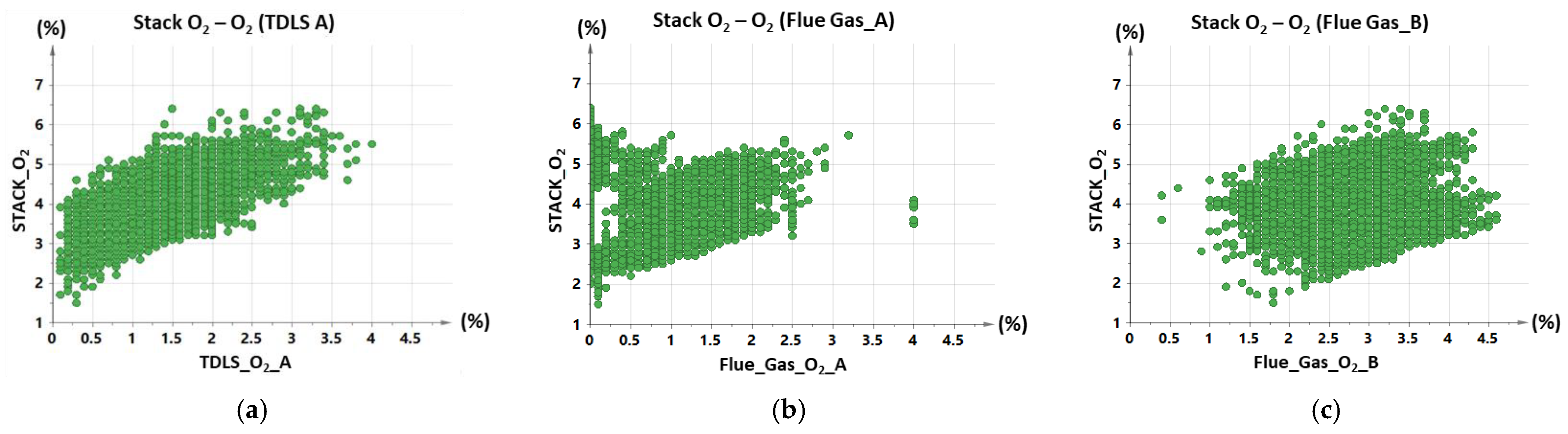
3.2.1. Feature Selection
3.2.2. Data Cleansing and Derived Variable Creation
4. Boiler Flue Gas Prediction Model (BFG-PM)
4.1. Model Selection
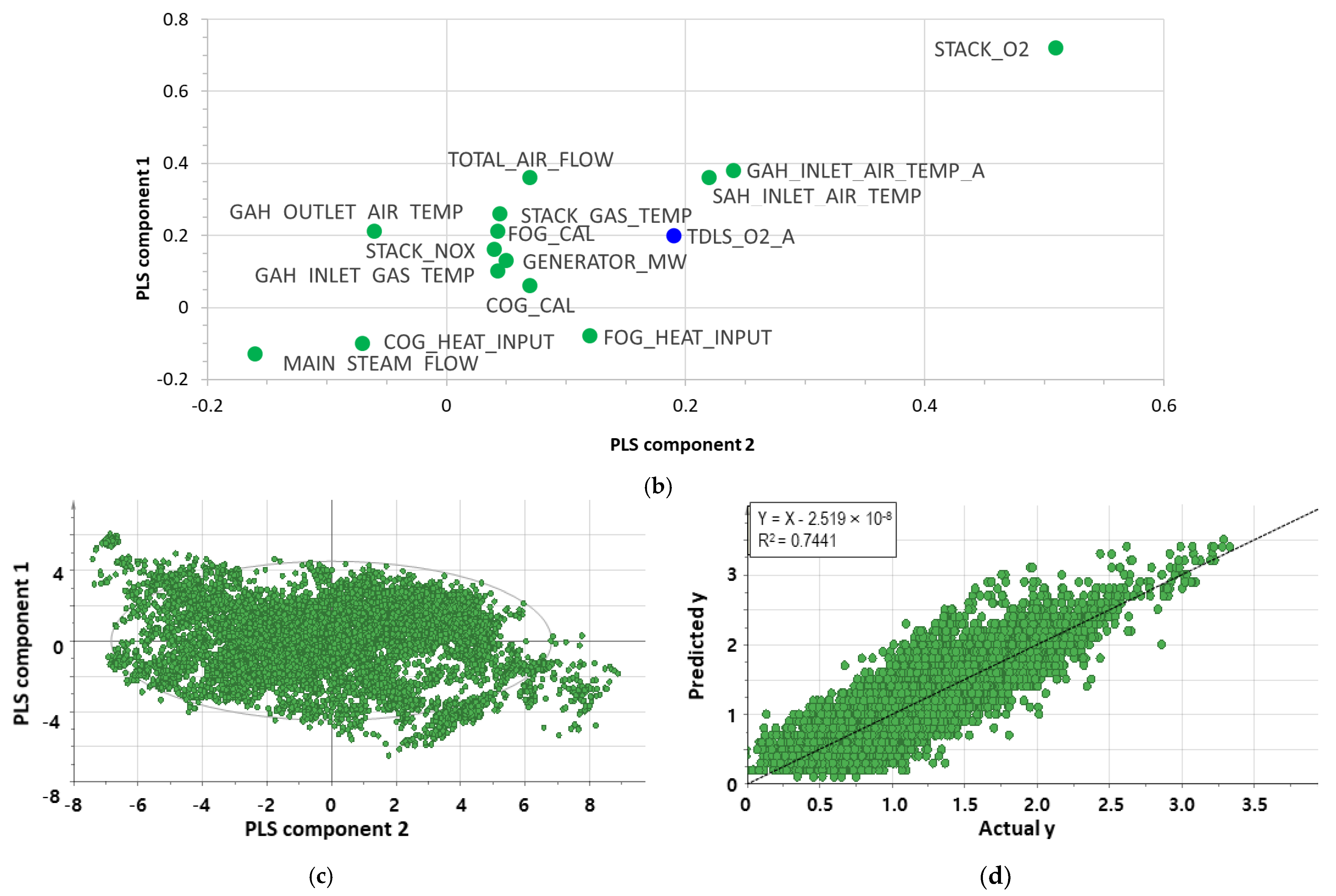
4.2. Modeling for Flue Gas Prediction
- K is the total number of signal variables
- wnk is the weight of the kth variable for the nth PLSR component
- N is the total number of PLSR components
- SSn is the sum of squares explained by the nth PLSR component.
5. Model Implementation and Validation
5.1. Model Implementation for Boiler Flue Gas O2
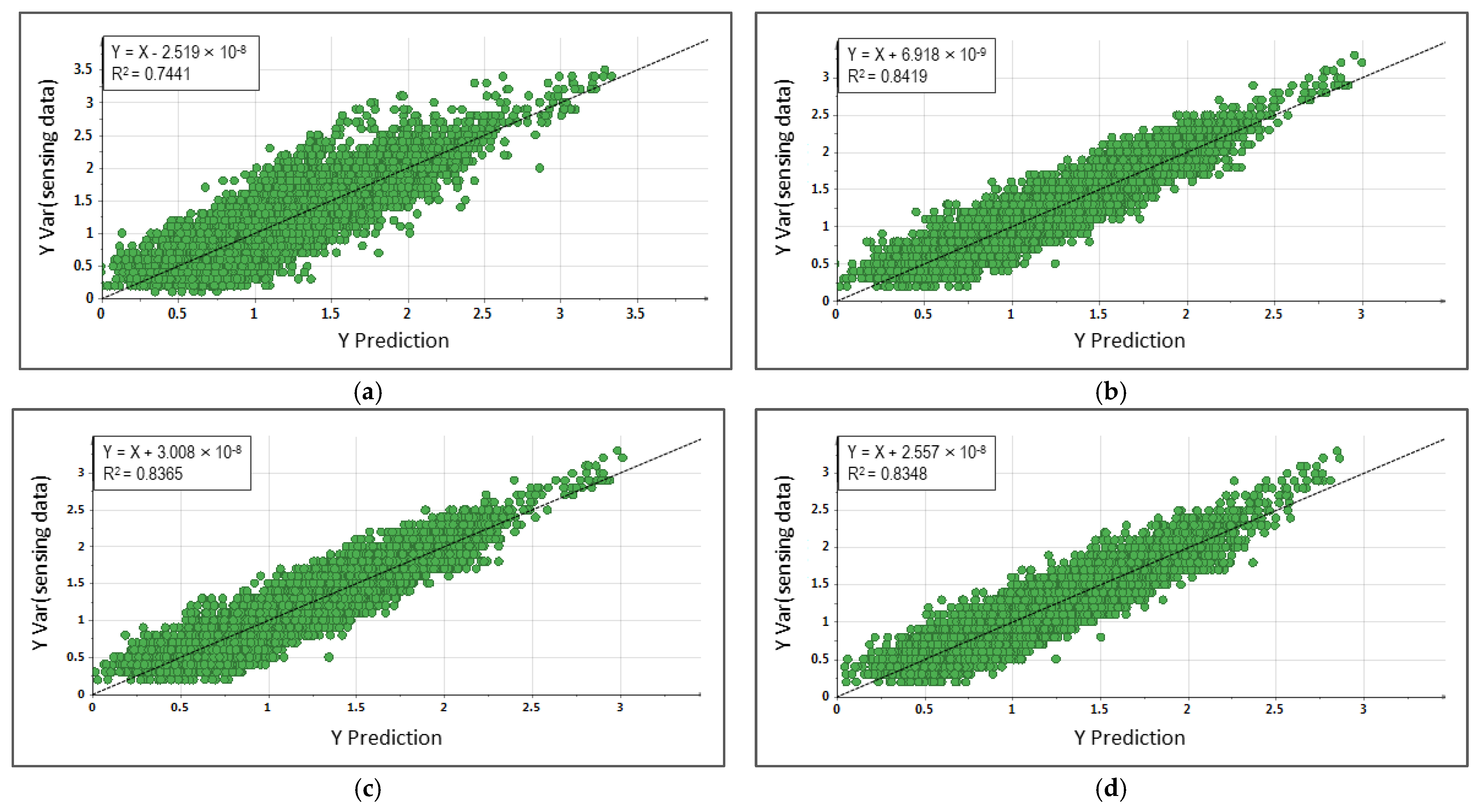
5.1.1. Training of BFG-PM for O2
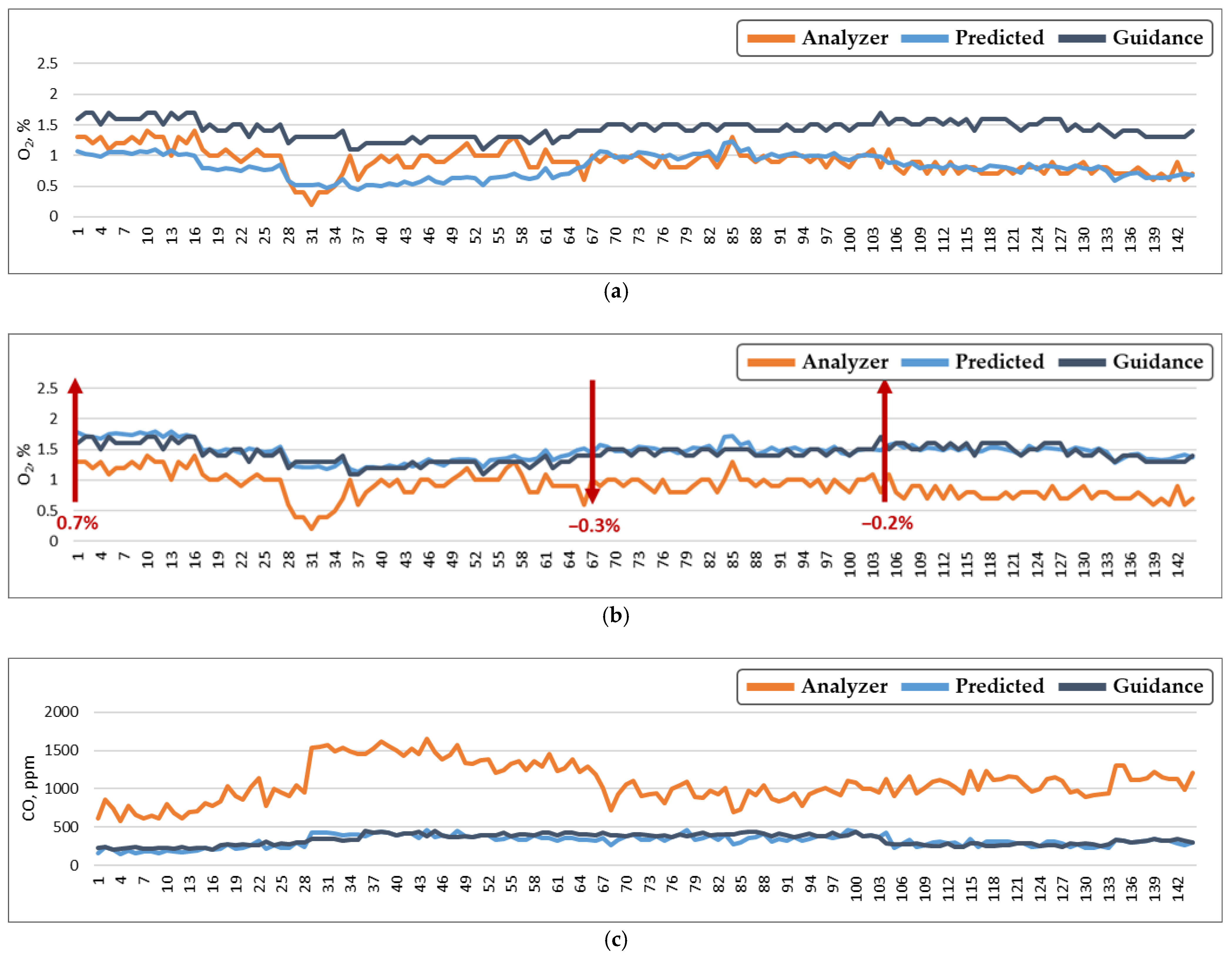
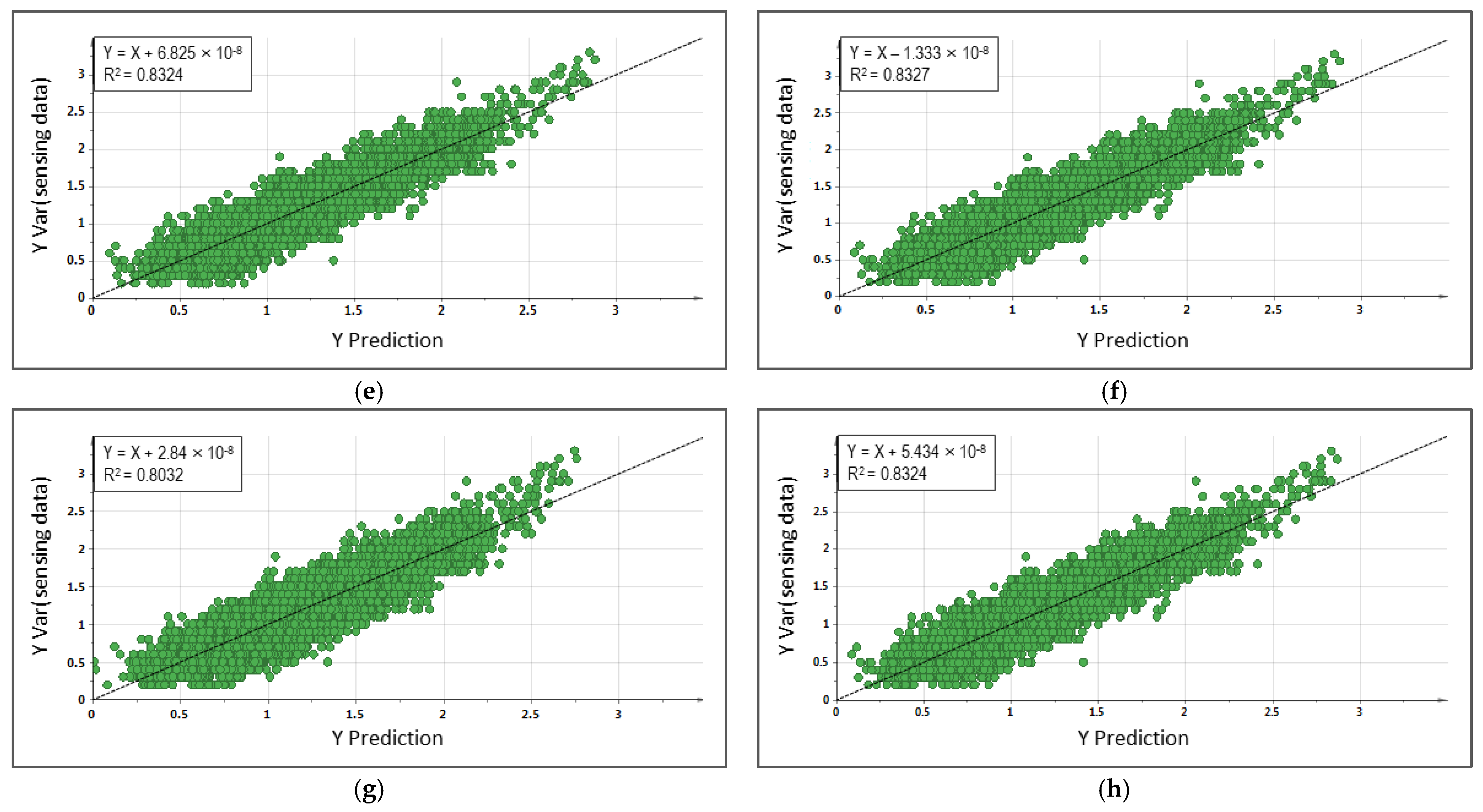
5.1.2. Implementation and Validation
5.2. Model Implementation for Boiler Flue Gas CO
5.2.1. Training of BFG-PM for CO
5.2.2. Implementation and Validation
5.3. Discussion
6. Combustion Efficiency Optimization
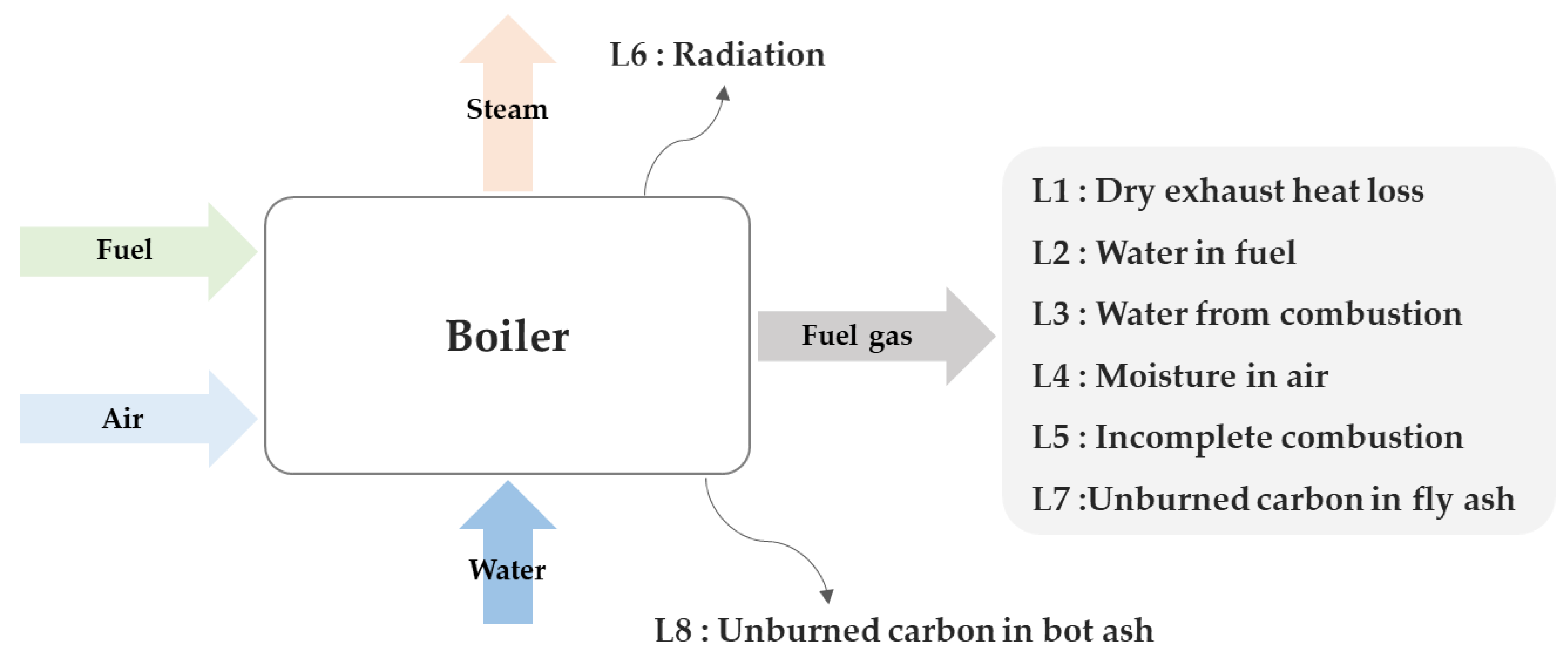
6.1. Select the Boiler Combustion Efficiency Calculation
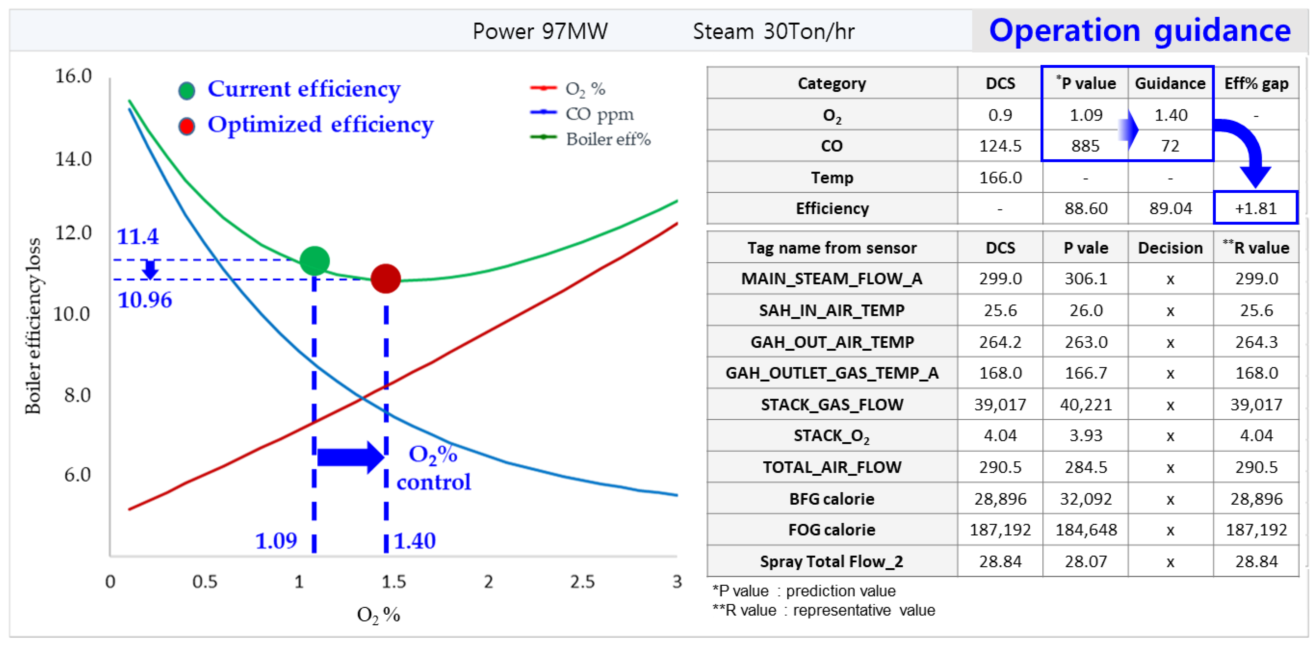
6.2. Efficiency Optimization
- Y represents CO ppm
- X represents O2%.
7. Site Application for Case Study
7.1. Simulation for Combustion Control
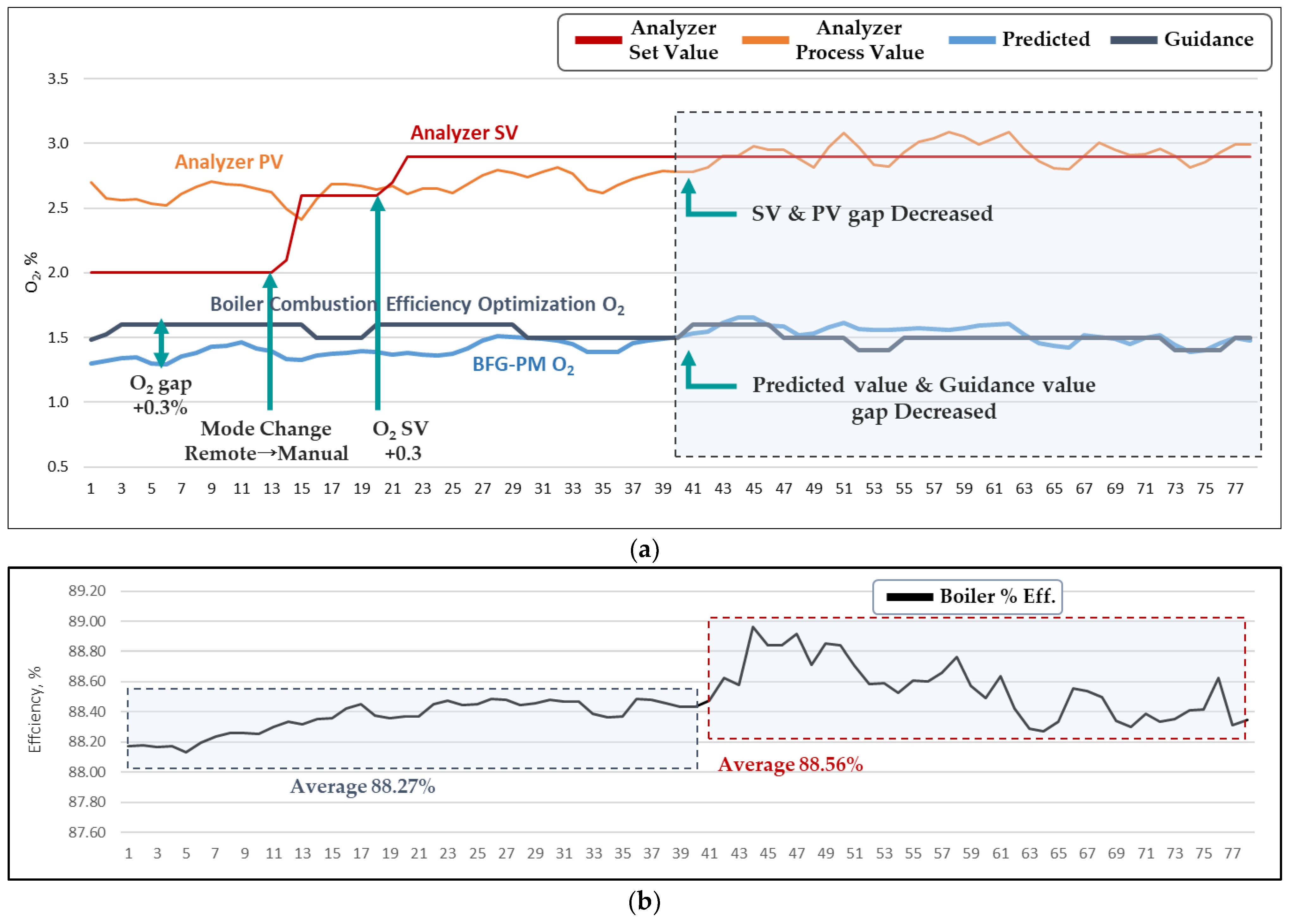
7.2. Site Application and Result
8. Benefits Analysis
9. Summary
9.1. Conclusions and Contributions
9.2. Limitations and Future Works
Author Contributions
Funding
Institutional Review Board Statement
Informed Consent Statement
Data Availability Statement
Acknowledgments
Conflicts of Interest
Abbreviations
| ANN | Artificial neural network |
| ASME | American Society of Mechanical Engineers |
| BFG | Blast furnace gas |
| BFG-PM | Boiler Flue Gas Prediction Model |
| BOP | Balance of plant |
| CFD | Computational Fluid Dynamics |
| CNN | Convolutional neural network |
| COG | Coke oven gas |
| DBN | Deep belief network |
| ESG | Environment, Social, Governance |
| FOG | FINEX off gas |
| GA | Genetic Algorithm |
| GAH | Gas Air Heater |
| GP | Gaussian Process |
| IoT | Internet of things |
| KNN | K Nearest Neighbors |
| LDG | Linz-donawiz converter gas |
| LSFLN | Least Square Fast Learning Network |
| LS-SVM | Least-Squares Support Vector Machine |
| LSTM | Long Short-Term Memory |
| MES | Manufacturing Execution System |
| ML | Machine Learning |
| NSGA | Non-dominated Sorting Genetic Algorithm |
| PLS | Partial Least Square |
| PLSR | Partial Least Square Regression |
| PTC | Performance Test Code |
| SVM | Support Vector Machine |
| TDLS | Tunable Diode Laser Spectrometer |
| VIP | Variable Importance in Projection |
References
- KEPC. Korean Electricity Bill. Available online: https://cyber.kepco.co.kr/ckepco/front/jsp/CY/E/E/CYEEHP00103.jsp (accessed on 21 August 2023).
- POSCO. Corporate Citizenship Report 2021. Available online: https://www.posco.co.kr/homepage/docs/eng7/jsp/irinfo/irdata/s91b6000030l.jsp (accessed on 21 August 2023).
- Ventrapati, T.; Rao, B. Efficiency and cost-benefit assessments on a typical 600MW coalfired boiler power plant. IJMPERD 2019, 9, 201–206. [Google Scholar] [CrossRef]
- POSRI. Improving Sustainable Competitiveness in Preparation for a Circular Economy: The Case of POSCO. Available online: https://www.posri.re.kr/files/file_pdf/59/342/6926/59_342_6926_file_pdf_1531111132.pdf (accessed on 21 August 2023).
- Babak, V.; Mokiychuk, V.; Zaporozhets, A.; Redko, O. Improving the efficiency of fuel combustion with regard to the uncertainty of measuring oxygen concentration. East.-Eur. J. Enterp. Technol. 2016, 6, 54–59. [Google Scholar] [CrossRef]
- Xiao, G.; Gao, X.; Lu, W.; Liu, X.; Asghar, A.B.; Jiang, L.; Jing, W. A physically based air proportioning methodology for optimized combustion in gas-fired boilers considering both heat release and NOx emissions. Appl. Energy 2023, 350, 121800. [Google Scholar] [CrossRef]
- Nemitallah, M.A.; Nabhan, M.A.; Alowaifeer, M.; Haeruman, A.; Alzahrani, F.; Habib, M.A.; Elshafei, M.; Abouheaf, M.I.; Aliyu, M.; Alfarraj, M. Artificial intelligence for control and optimization of boilers’ performance and emissions: A review. J. Clean. Prod. 2023, 417, 138109. [Google Scholar] [CrossRef]
- Bartnicki, G.; Klimczak, M.; Ziembicki, P. Evaluation of the effects of optimization of gas boiler burner control by means of an innovative method of Fuel Input Factor. Energy 2023, 263, 125708. [Google Scholar] [CrossRef]
- Santoso, H.; Ariwibowo, T.H.; Safitra, A.G. Effect of Air-Fuel Ratio to Non-premixed Burning Characteristics in Boiler Furnace Using CFD. In Proceedings of the Seminar Nasional Tahunan Teknik Mesin (SNTTM) XVI, Surabaya, Indonesia, 5–6 October 2017; pp. 92–98. [Google Scholar]
- Pryiomov, S.; Shybetskyi, V.; Plashykhin, S.; Kostyk, S.; Safiants, A.S.; Romanova, K.; Nizhnyk, N. Increasing the energy efficiency of cyclone dust collectors. IJECE 2023, 24, 81–96. [Google Scholar] [CrossRef]
- Murehwa, G.; Zimwara, D.; Tumbudzuku, W.; Mhlanga, S. Energy efficiency improvement in thermal power plants. IJITEE 2012, 2, 20–25. [Google Scholar]
- Karri, V.S.S.K. A Theoretical Investigation of Efficiency Enhancement in Thermal Power Plants. Mod. Mech. Eng. 2012, 2, 106–113. [Google Scholar] [CrossRef]
- Mandi, R.P.; Yaragatti, U.R. Energy efficiency improvement of auxiliary power equipment in thermal power plant through operational optimization. In Proceedings of the Power Electronics, Drives and Energy Systems (PEDES), Bengaluru, India, 16–19 December 2012; pp. 1–8. [Google Scholar]
- Hasanuzzaman, M.; Rahim, N.A.; Hosenuzzaman, M.; Saidur, R.; Mahbubul, I.M.; Rashid, M.M. Energy savings in the combustion based process heating in industrial sector. Renew. Sust. Energ. Rev. 2012, 16, 4527–4536. [Google Scholar] [CrossRef]
- Ibrahim, T.k.; Mohammed, M.K.; Awad, O.I.; Rahman, M.M.; Najafi, G.; Basrawi, F.; Abd Alla, A.N.; Mamat, R. The optimum performance of the combined cycle power plant: A comprehensive review. Renew. Sust. Energ. Rev. 2017, 79, 459–474. [Google Scholar] [CrossRef]
- Errami, Y.; Obbadi, A.; Sahnoun, S.; Ouassaid, M.; Maaroufi, M. Performance evaluation of backstepping approach for wind power generation system-based permanent magnet synchronous generator and operating under non-ideal grid voltages. Int. J. Power Energy Convers. 2019, 10, 414–451. [Google Scholar] [CrossRef]
- Mosobi, R.W.; Gao, S. Power quality analysis of low voltage distributed generators in standalone and grid connected modes. Int. J. Power Energy Convers. 2021, 12, 267–293. [Google Scholar] [CrossRef]
- Khaleel, O.J.; Ibrahim, T.K.; Ismail, F.B.; Al-Sammarraie, A.T.; bin Abu Hassan, S.H. Modeling and analysis of optimal performance of a coal-fired power plant based on exergy evaluation. Energy Rep. 2022, 8, 2179–2199. [Google Scholar] [CrossRef]
- Zaporozhets, A. Development of software for fuel combustion control system based on frequency regulator. In Proceedings of the ICT in Education, Research, and Industrial Applications (ICTERI) 2019, Kherson, Ukraine, 12–15 June 2019; pp. 12–15. [Google Scholar]
- Tang, Z.; Li, Y.; Kusiak, A. A deep learning model for measuring oxygen content of boiler flue gas. IEEE Access 2020, 8, 12268–12278. [Google Scholar] [CrossRef]
- Pan, H.; Su, T.; Huang, X.; Wang, Z. LSTM-based soft sensor design for oxygen content of flue gas in coal-fired power plant. Trans. Inst. Meas. Control 2021, 43, 78–87. [Google Scholar] [CrossRef]
- Effendy, N.; Kurniawan, E.D.; Dwiantoro, K.; Arif, A.; Muddin, N. The prediction of the oxygen content of the flue gas in a gas-fired boiler system using neural networks and random forest. IJ-AI 2022, 11, 923–929. [Google Scholar] [CrossRef]
- Li, Z.; Li, G.; Shi, B. Prediction of Oxygen Content in Boiler Flue Gas Based on a Convolutional Neural Network. Processes 2023, 11, 990. [Google Scholar] [CrossRef]
- Santoso, H.M.; Nazaruddin, Y.Y.; Muchtadi, F.I. Boiler performance optimization using fuzzy logic controller. IFAC Proc. Vol. 2005, 38, 308–313. [Google Scholar] [CrossRef]
- Liu, X.; Bansal, R. Integrating multi-objective optimization with computational fluid dynamics to optimize boiler combustion process of a coal fired power plant. Appl. Energy 2014, 130, 658–669. [Google Scholar] [CrossRef]
- Li, G.; Niu, P.; Wang, H.; Liu, Y. Least Square Fast Learning Network for modeling the combustion efficiency of a 300WM coal-fired boiler. Neural Netw. 2014, 51, 57–66. [Google Scholar] [CrossRef]
- Suntivarakorn, R.; Treedet, W. Improvement of boiler’s efficiency using heat recovery and automatic combustion control system. Energy Procedia 2016, 100, 193–197. [Google Scholar] [CrossRef]
- Wang, C.; Liu, Y.; Zheng, S.; Jiang, A. Optimizing combustion of coal fired boilers for reducing NOx emission using Gaussian Process. Energy 2018, 153, 149–158. [Google Scholar] [CrossRef]
- Shi, Y.; Zhong, W.; Chen, X.; Yu, A.; Li, J. Combustion optimization of ultra supercritical boiler based on artificial intelligence. Energy 2019, 170, 804–817. [Google Scholar] [CrossRef]
- Niu, Y.; Kang, J.; Li, F.; Ge, W.; Zhou, G. Case-based reasoning based on grey-relational theory for the optimization of boiler combustion systems. ISA Trans. 2020, 103, 166–176. [Google Scholar] [CrossRef] [PubMed]
- Vieira, L.W.; Marques, A.D.; Schneider, P.S.; da Silva Neto, A.J.; Viana, F.A.C.; Abdel-jawad, M.; Hunt, J.D.; Siluk, J.C.M. Methodology for ranking controllable parameters to enhance operation of a steam generator with a combined Artificial Neural Network and Design of Experiments approach. Energy AI 2021, 3, 100040. [Google Scholar] [CrossRef]
- Murdoch, W.J.; Singh, C.; Kumbier, K.; Abbasi-Asl, R.; Yu, B. Definitions, methods, and applications in interpretable machine learning. Proc. Natl. Acad. Sci. USA 2019, 116, 22071–22080. [Google Scholar] [CrossRef] [PubMed]
- Vergara, J.R.; Estévez, P.A. A review of feature selection methods based on mutual information. Neural. Comput. Appl. 2014, 24, 175–186. [Google Scholar] [CrossRef]
- Chen, T.; Martin, E.; Montague, G. Robust probabilistic PCA with missing data and contribution analysis for outlier detection. CSDA 2009, 53, 3706–3716. [Google Scholar] [CrossRef]
- Ryu, S.-E.; Shin, D.-H.; Chung, K. Prediction model of dementia risk based on XGBoost using derived variable extraction and hyper parameter optimization. IEEE Access 2020, 8, 177708–177720. [Google Scholar] [CrossRef]
- Abdulqader, D.M.; Abdulazeez, A.M.; Zeebaree, D.Q. Machine learning supervised algorithms of gene selection: A review. Mach. Learn. 2020, 62, 233–244. [Google Scholar]
- Choi, S.W.; Lee, I.-B. Multiblock PLS-based localized process diagnosis. J. Process Control 2005, 15, 295–306. [Google Scholar] [CrossRef]
- Wold, S.; Sjöström, M.; Eriksson, L. PLS-regression: A basic tool of chemometrics. Chemom. Intell. Lab. Syst. 2001, 58, 109–130. [Google Scholar] [CrossRef]
- Ding, J.G.; He, Y.H.C.; Kong, L.P.; Peng, W. Camber prediction based on fusion method with mechanism model and machine learning in plate rolling. ISIJ Int. 2021, 61, 2540–2551. [Google Scholar] [CrossRef]
- Zhong, F.; Liu, X.; Zhou, Q.; Hao, X.; Lu, Y.; Guo, S.; Wang, W.; Lin, D.; Chen, N. 1H NMR spectroscopy analysis of metabolites in the kidneys provides new insight into pathophysiological mechanisms: Applications for treatment with Cordyceps sinensis. Nephrol. Dial. Transplant. 2012, 27, 556–565. [Google Scholar] [CrossRef] [PubMed]
- Farrés, M.; Platikanov, S.; Tsakovski, S.; Tauler, R. Comparison of the variable importance in projection (VIP) and of the selectivity ratio (SR) methods for variable selection and interpretation. J. Chemom. 2015, 29, 528–536. [Google Scholar] [CrossRef]
- Hastie, T.; Tibshirani, R.; Friedman, J.H.; Friedman, J.H. The Elements of Statistical Learning: Data Mining, Inference, and Prediction, 2nd ed.; Springer: New York, NY, USA, 2009; Volume 2. [Google Scholar] [CrossRef]
- Purseth, S.; Dansena, J.; Desai, M.S. Performance analysis and efficiency improvement of boiler—A review. IJEAST 2021, 5, 326–331. [Google Scholar] [CrossRef]
- ASME PTC-4:2013 (Revision of ASME PTC 4-2008); Performance Test Code on Fired Steam Generators. ASME: New York, NY, USA, 2013.
- Behbahaninia, A.; Ramezani, S.; Hejrandoost, M.L. A loss method for exergy auditing of steam boilers. Energy 2017, 140, 253–260. [Google Scholar] [CrossRef]
- KEPC. Electricity Supply Terms and Conditions. Available online: https://cyber.kepco.co.kr/ckepco/front/jsp/CY/D/C/CYDCHP00401.jsp (accessed on 21 August 2023).


| Category | BFG 1 | COG 2 | LDG 3 | FOG 4 | |
|---|---|---|---|---|---|
| Standard calorie (Kcal/Nm3) | 750 | 4400 | 2000 | 1350 | |
| Specific gravity | 1.03 | 0.42 | 1.04 | 1.38 | |
| Component (%) | CO2 | 20.7 | 3.1 | 17.8 | 33 |
| O2 | - | 0.3 | - | - | |
| C2H4 | - | 2.0 | - | - | |
| CO | 20.0 | 8.4 | 64.2 | 43 | |
| CH4 | - | 26.6 | - | 1 | |
| H2 | 3.2 | 56.4 | 2.0 | 21 | |
| N2 | 54.1 | 2.3 | 15.9 | 2 | |
| Category | Methods/Tools Used for Efficiency Improvement | Year | Authors |
|---|---|---|---|
| Conventional efficiency improvement | Exergy analysis | 2012 | Murehwa et al. [11] |
| Flue gas temperature drop | 2012 | Karri [12] | |
| Flue gas pressure drop and induced draft fan overhaul | 2012 | Mandi et al. [13] | |
| Air pre-heating using recuperator | 2012 | Hasanuzzaman et al. [14] | |
| Parametric analysis and simulation model | 2017 | Ibrahim et al. [15] | |
| Nonlinear control strategy based on nonlinear backstepping theory | 2019 | Errami et al. [16] | |
| System development by integrating PVS, WEGS, and MHGS | 2021 | Mosobi and Gao [17] | |
| Modeling through exergy evaluation | 2022 | Khaleel et al. [18] | |
| Prediction of flue gas | Flue gas O2 monitoring using linear model programming | 2019 | Zaporozhets [19] |
| LASSO algorithm, deep belief network, and least squares support vector machine | 2020 | Tang et al. [20] | |
| Long short-term memory modeling | 2020 | Pan et al. [21] | |
| Artificial neural network and random forest-based soft sensor | 2022 | Effendy et al. [22] | |
| Convolutional neural network modeling | 2023 | Li et al. [23] | |
| Boiler combustion efficiency improvement | Reducing air with a fuzzy logic controller | 2005 | Santoso et al. [24] |
| Non-dominated sorting genetic algorithm and computational fluid dynamics | 2014 | Liu et al. [25] | |
| Least square fast learning network | 2014 | Li et al. [26] | |
| Auto-combustion control system using a fuzzy logic control algorithm | 2016 | Suntivarakorn et al. [27] | |
| Gaussian process and genetic algorithm | 2018 | Wang et al. [28] | |
| Artificial neural network and computational fluid dynamics | 2019 | Shi et al. [29] | |
| Least squares support vector machine | 2020 | Niu et al. [30] | |
| Artificial neural network | 2021 | Vieira et al. [31] |
| Category | Class | Features | Number of Features |
|---|---|---|---|
| Boiler (167) | Fuel combustion system boiler | Including BFG/COG/FOG calorie, BFG/COF/FOG flow control, TDLS O2/CO, flue gas O2, flue gas inlet/outlet temp, total fuel flow, total air flow control | 54 |
| Heat exchange equipment | Including GAH inlet/outlet gas temp, GAH oil pump temp, FSH inlet/outlet steam temp, HPH inlet/outlet fw temp | 29 | |
| High-pressure steam boiler | Including FDF wind temp, FDF fan BRG temp, FDF motor BRG temp, AUX process steam temp, AUX steam head temp, STACK GAS flow, STACK_O2, main steam flow, process steam flow | 60 | |
| Water supply system boiler | Including platen SH inlet V/V, platen SH out V/V, BFP wind temp, BFP suction FW PH, BFP motor BRG temp | 24 | |
| Generator (13) | Generator | generator watt, generator mvar, generator zero phase current, gfr fluid oil press | 4 |
| Drive system | Including FDF/IDF VVVF output ampere, FDF/IDF VVVF output voltage, FDF/IDF VVVF RPM | 9 | |
| Balance of Plant (BOP) (187) | Condenser system | Including BCW CLR inlet/outlet temp, BCW PH, BCW pump outlet pressure, COND overflow control valve, COND pump recirculation control valve | 13 |
| High-voltage power equipment | Including 6.6 kV unit BUS ampere, 6.6 kV unit BUS VAR, ESP unit main TR BCT Ao, main TR wind temp, unit AUX TR current, unit TR oil temp | 24 | |
| Low voltage power equipment | Including battery charger DC out current, battery charger battery current, 440 V unit BUS watt | 6 | |
| Steam turbine | Including turning speed, turning motor current, turbine inlet steam press, turbine inlet steam temp, cold air exit temp, exciter current, exciter voltage | 96 | |
| Water treatment system | including make up water tank level, make up pump ampere, raw water pump out flow, degasifier clear water level | 48 | |
| Total | 361 | ||
| Category | Types | Decision | Characteristic | Advantages | Disadvantage |
|---|---|---|---|---|---|
| Linear regression | Regression | Linear | Finding best straight line | Simple model easy /Implementation and interpretation | Poor prediction on non-linear |
| Logistic regression | Classification | Linear | Binary classification /Categorical prediction /Comparison of other models | Simple model /easy implementation and interpretation | Poor prediction in non-linear |
| 1 KNN | Regression/Classification | Non Small outlier | Identification a new data | Easy multi- Classification /Intuition and Simple | Vulnerable to outliers /Slow on big data |
| 2 SVM | Regression/Classification | Linear/ Non-Linear | Classification of 2 or more groups | Categorical numerical prediction /Low impact on error data, Less overfitting | Multiple combination tests required /Slow to learn /Difficult interpretation |
| 3 PLSR | Regression/Classification | Linear | Considers input and output variables together | Easy control of multi-collinearity /Variable reduction with correlation /Efficient model construction | Difficult interpretation of extracted variables |
| Component | R2X | R2Y |
|---|---|---|
| 1 | 0.283 | 0.282 |
| 2 | 0.469 | 0.413 |
| 3 | 0.524 | 0.657 |
| 4 | 0.681 | 0.690 |
| 5 | 0.806 | 0.721 |
| 6 | 0.867 | 0.744 |
| Category | Variables | Components | R2X | R2Y | Model Selection |
|---|---|---|---|---|---|
| 1st training | 33 | 6 | 0.867 | 0.744 | |
| 2nd training | 17 | 5 | 0.925 | 0.842 | |
| 3rd training | 13 | 4 | 0.764 | 0.836 | |
| 4th training | 12 | 5 | 0.930 | 0.835 | |
| 5th training | 11 | 6 | 0.976 | 0.832 | |
| 6th training | 9 | 6 | 0.974 | 0.833 | |
| 7th training | 8 | 7 | 0.992 | 0.832 | *✓ |
| 8th training | 7 | 4 | 0.945 | 0.803 |
| Category | O2 Prediction | |
|---|---|---|
| R2Y | 0.832 | |
| Acceptance criteria | O2 gap between actual and prediction ±0.25% | |
| Result | 90.89% | |
| Within standard | 5199 ea | 90.89% |
| Out of standard | 521 ea | 9.11% |
| Total | 5720 ea | 100% |
| Category | Variables | Components | R2X | R2Y | Model Selection |
|---|---|---|---|---|---|
| 1st training | 33 | 5 | 0.750 | 0.453 | |
| 2nd training | 17 | 10 | 0.976 | 0.543 | |
| 3rd training | 14 | 9 | 0.990 | 0.536 | |
| 4th training | 11 | 9 | 0.995 | 0.477 | |
| 5th training | 13 | 9 | 0.993 | 0.534 | |
| 6th training | 12 | 8 | 0.992 | 0.532 | |
| 7th training | 10 | 4 | 0.753 | 0.375 | |
| 8th training | 11 | 8 | 0.993 | 0.534 | *✓ |
| 9th training | 9 | 5 | 0.873 | 0.380 |
| Category | CO Prediction | |
|---|---|---|
| R2Y | 0.534 | |
| Acceptance criteria | CO gap between actual and prediction ±350 ppm | |
| Result | 90.09% | |
| Within standard | 9869 ea | 90.09% |
| Out of standard | 1086 ea | 9.91% |
| Total | 10,955 ea | 100% |
| Loss Calculation | Equations |
|---|---|
| Loss 1, Dry exhaust heat loss | ((0.981790389084853 × B12 − 0.82499216637857 × B13 + 0.905867445657761 × B14) + (1 + B4/(21 − B4)) × (0.595123830015147 × B12 + 11.3028230711785 × B13 + 1.04479223434223 × B14)) × (1.38906921002696 × B12 + 0.492352550459239 × B13 + 1.38823214285714 × B14) × (B3-B7)/((B12 + B13 + B14) × (B9 × B12 + B10 × B13 + B11 × B14)) × 23 |
| Loss 2, Water in fuel | - |
| Loss 3, Water from combustion | 4.05 × (0.201568899331099 × B12 + 20.263286732307 × B13 + 1.04449389639958 × B14)/(B12 + B13 + B14) × (B3B7)/((B9 × B12 + B10 × B13 + B11 × B14)/(1.38906921002696 × B12 + 0.492352550459239 × B13 + 1.38823214285714 × B14)) |
| Loss 4, Moisture in the air | (1 + B4/(21 − B4)) × (59.512383006586 × B12 + 1130.28230712112 × B13 + 104.479232322713 × B14)/(B12 + B13 + B14) × B8 × 0.45 × (B3 − B7)/((B9 × B12 + B10 × B13 + B11 × B14)/(1.38906921002696 × B12 + 0.492352550459239 × B13 + 1.38823214285714 × B14)) |
| Loss 5, Incomplete combustion | B5/(B5 + B6) × (18.6804298424681 × B12 + 43.3664332479575 × B13 + 27.9736561145342 × B14)/(B12 + B13 + B14) × 5744/((B9 × B12 + B10 × B13 + B11 × B14)/(1.38906921002696 × B12 + 0.492352550459239 × B13 + 1.38823214285714 × B14)) |
| Loss 6, Radiation | 0.50 |
| Loss 7, Unburned carbon in fly ash | - |
| Loss 8, Unburned carbon in bot ash | - |
| O2 prediction | 0.2 | 0.4 | 0.6 | 0.8 | 1.0 | 1.2 | 1.4 | 1.5 | 1.6 | 1.8 | 2.0 | 2.2 | 2.4 |
| CO prediction | 1508 | 1234 | 1011 | 827 | 677 | 555 | 454 | 411 | 372 | 304 | 249 | 204 | 167 |
| %Eff | 89.43 | 89.56 | 89.65 | 89.72 | 89.76 | 89.79 | 89.81 | 89.81 | 89.81 | 89.80 | 89.78 | 89.76 | 89.73 |
| Category | Calculation Result |
|---|---|
| Energy cost | 89 MW × 0.29% × 24 h/day × 365 day/year × 96% × 1000 kWh/MWh × USD 0.1/kWh = USD 217,000/year (KRW 2.74B/year) |
| The cost of emission trading | 89 MW × 0.29% × 24 h/day × 365 day/year × 96% × 0.4781 tCO2eq/MWh × USD 19/* tCO2eq = USD 19,700/year (KRW 0.25B/year) |
Disclaimer/Publisher’s Note: The statements, opinions and data contained in all publications are solely those of the individual author(s) and contributor(s) and not of MDPI and/or the editor(s). MDPI and/or the editor(s) disclaim responsibility for any injury to people or property resulting from any ideas, methods, instructions or products referred to in the content. |
© 2023 by the authors. Licensee MDPI, Basel, Switzerland. This article is an open access article distributed under the terms and conditions of the Creative Commons Attribution (CC BY) license (https://creativecommons.org/licenses/by/4.0/).
Share and Cite
Lee, S.-M.; Choi, S.-W.; Lee, E.-B. Prediction Modeling of Flue Gas Control for Combustion Efficiency Optimization for Steel Mill Power Plant Boilers Based on Partial Least Squares Regression (PLSR). Energies 2023, 16, 6907. https://doi.org/10.3390/en16196907
Lee S-M, Choi S-W, Lee E-B. Prediction Modeling of Flue Gas Control for Combustion Efficiency Optimization for Steel Mill Power Plant Boilers Based on Partial Least Squares Regression (PLSR). Energies. 2023; 16(19):6907. https://doi.org/10.3390/en16196907
Chicago/Turabian StyleLee, Sang-Mok, So-Won Choi, and Eul-Bum Lee. 2023. "Prediction Modeling of Flue Gas Control for Combustion Efficiency Optimization for Steel Mill Power Plant Boilers Based on Partial Least Squares Regression (PLSR)" Energies 16, no. 19: 6907. https://doi.org/10.3390/en16196907
APA StyleLee, S.-M., Choi, S.-W., & Lee, E.-B. (2023). Prediction Modeling of Flue Gas Control for Combustion Efficiency Optimization for Steel Mill Power Plant Boilers Based on Partial Least Squares Regression (PLSR). Energies, 16(19), 6907. https://doi.org/10.3390/en16196907