Article

Parameter-Free Model Predictive Current Control for PMSM Based on Current Variation Estimation without Position Sensor

School of Electrical Engineering, Nantong University, Nantong 226019, China
*
Author to whom correspondence should be addressed.
Energies 2023, 16(19), 6792; https://doi.org/10.3390/en16196792
Submission received: 23 August 2023 / Revised: 14 September 2023 / Accepted: 20 September 2023 / Published: 24 September 2023

Abstract

:
To remove parameter dependence in existing sensorless control strategies, a parameter-free model predictive current control is proposed for permanent magnet synchronous motor without any position sensor. First, the current variation during one sampling period is analyzed and divided into two elements: natural attenuation and forced response. Second, recursive least squares algorithm is utilized to estimate the future current variation so that the model predictive current control can be successfully executed paying no attention to motor parameters. Meanwhile, the position information is obtained by the arc tangent function according to the estimated forced response of current variation. At last, experimental results verify that the estimation errors of rotor position are reduced to around 0.1 rad with smaller current prediction error even at low speed where no motor parameters are required.

1. Introduction

Permanent magnet synchronous motor (PMSM) is identified as a high-performance exchange motor. It has played an irreplaceable role in industrial and civil production [1]. Nowadays, its control technology is always evolving owing to the advancement of motion control theory, power electronics technology and sensor design. Model predictive control (MPC) strategy is viewed as a promising way to replace the PI modem, directly taking into account the nonlinearity and constraint characteristics of the system [2,3]. Depending on the operation principle, MPC can be classified into two categories, namely the continuous control set MPC (CCS-MPC) and the finite control set MPC (FCS-MPC). Specifically, the FCS-MPC strategy directly tracks the reference states through the enumeration of possible switching states, so that the applied switching state for inverter can be decided simply [4,5]. In this manner, the external modulation stages are avoided, which is an indispensable part of CCS-MPC [6]. At present, model predictive current control (MPCC) has been widely used with the aim to predict future currents.
In practical applications, high-precision sensors increase the design cost of the control system, and the mechanical encoders desire additional assembly space and system maintenance. In addition, the stability of communication between the encoder and the motor drive is inevitably affected by external signals and noise. Moreover, when the sensors are installed in a PMSM with low moment of inertia, rotational inertia of rotor increases incurring the deteriorative robustness [7,8,9]. In addition, in some more complex operating environments, the motor drive system ensures the safety and stability of the system in addition to ensuring high dynamic responsiveness and gauge stability. Position sensors are a common part of the motor control system failure, and in some cases can be replaced by sensorless control technology [10].
In principle, the positionless sensing program can be generally divided into two categories: one is a program based on the electromagnetic variation relationship in a mathematical model, and the other is a position estimation strategy based on a PMSM emphasis effect. The former can be subdivided into an open-circle calculation program based upon an ideal model and a closed-circuit calculation method based on an observer [11], while the latter is typically based on high-frequency injection methods based on non-ideal properties achieved [12]. Many sensorless control methods are in conjunction with MPCC. Refs. [13,14,15] put effort into high-frequency information injection to identify the rotor speed, which takes advantage of unequal quadrature- and direct-axis inductance caused by inductance magnetic saturation effect. As a whole, high-frequency injection methods have some problems such as poor dynamic performance and reduced bandwidth. Also, the performance of applied power electronic device is critical.
Instead, refs. [16,17,18,19,20] advocate for the design of observers that function to estimated rotor position. In [16], an adaptive full-order observer is adopted to smoothly start a free-running motor without any position sensors. The feedback gain matrix is conceived to realize that the estimated speed can trace the actual value even if the initial difference is large. On the contrary, the rotor position is estimated via a disturbance observer in [17], and the estimation error is effectively reduced by considering the iron loss. Even in the quadrotor system, observers like finite-time extended state observer and adaptive neural network observer are adopted to estimate the position information [18]. In addition, the sliding mode observer (SMO) and the full-order state observer are utilized in the sensorless control of [19,20], respectively. Nonetheless, it is worth mentioning that these sensorless control methods are dependent on the motor parameters, which fail to remain constant in all conditions owing to the variable operation environment [21,22]. Thus, the strategies with strong parameter robustness attract a lot of attention to keep the normal operation when parameters are mismatched [23].
Reference [24] analyzes the influence of parameter mismatch on the proposed sensorless method. The injected high-frequency voltage is viewed as the reference value and added into the cost function for voltage tracking. Therefore, the robustness against parameter mismatch is improved without any complicated work. On the premise of parameter-free MPCC based on the ultra-local model, ref. [25] builds a sliding mode observer for a sensorless driving system, and the prediction horizon can be adjusted online considering prediction error. An improved-position self-detecting observer is adopted in [26], where the estimation accuracy of rotor position is improved. Meanwhile, the parameter-adaptive SMO is devoted to suppressing the influence of motor parameter variation. It is obvious that most sensorless methods achieve parameter-free control owing to the observers. However, the application of observers indicates that the mathematical model of the motor is still indispensable in the control. For example, the ultralocal model in [24] predicts the future current by virtue of inductance parameters. Moreover, when more observers participate in the control, the increased complexity of the system is accompanied by heavy tuning work.
To completely get rid of the dependence of motor parameters in position-free control, the current variations corresponding to active voltage vectors are dissected in this paper, based on which the prediction of future current and rotor position estimation are achieved via the current variations obtained from the recursive least squares (RLS) algorithm. The contributions of this paper are summarized as follows:
  • Taking the current variations as the estimation target, a parameter-free MPCC is designed on the basis of RLS, where the natural attenuation and forced response of current variations are estimated accurately. It successfully avoids the effects of lost initial data in [25] and the problem of current variation renewal stagnates in [23].
  • To estimate the rotor position through the known current variations, the forced response value is analyzed together with the active voltage vector, after which an accurate rotor position angle can be obtained by the built arc tangent function. Parameter dependence in [24,26] is successfully overcome.
  • Both simulated and experimental results verify the correctness and effectiveness of the proposed method.
The remainder of article is organized as follows. The model of the PMSM drive system is provided in Section 2, where the current variation is analyzed carefully. In Section 3, the proposed sensorless parameter-free MPCC is revealed in terms of future current prediction and rotor position estimation. Afterwards, the experimental results verify the effectiveness and superiority of the proposed control strategy in Section 4. Finally, this study is concluded in Section 5.

2. Model of PMSM Drive System

2.1. Mathematical Model of Motor

For a convenient design of a controller, the mathematical model is usually built in synchronous rotating coordinates, so that the stator voltage of the concerned three-phase PMSM [24] can be obtained as
[ u d u q ] = [ R ω e L q ω e L d R ] [ i d i q ] + [ L d 0 0 L q ] d d t [ i d i q ] + [ 0 ω e ψ f ] ,
where u, i and L refer to the stator voltage, current and inductance, respectively. Subscripts d and q represent the corresponding components of these parameters in dq-axes. R, ωe and ψf denote the stator resistance, electrical angular velocity and permanent magnet flux linkage, respectively. In this paper, PMSM is driven by a traditional two-level inverter, which can produce eight voltage vectors as exhibited in Figure 1.

2.2. Model of Current Variations

By rearranging the stator voltage Equation (1), the differentials of dq-axes currents can be calculated as
d d t [ i d i q ] = [ R / L d ω e L q / L d ω e L d / L q R / L q ] [ i d i q ] + [ u d / L d u q ω e ψ f / L q ] .
Relying on the Forward Euler method, dq-axes currents in (k + 1)th are predicted as
[ i d ( k + 1 ) i q ( k + 1 ) ] = [ L d R T s L d L q ω e T s L d L q R T s L q L d ω e T s L q ] [ i d ( k ) i q ( k ) ] + [ T s L d u d ( k ) T s L q u q ( k ) ψ f ω e T s L q ] .
Therefore, the current variations between two consecutive sampling periods can be expressed as
[ Δ i d | V j Δ i q | V j ] = [ R T s / L d ω e L q T s / L d ω e L d T s / L q R T s / L q ] [ i d i q ] + [ 0 ω e ψ f T s / L q ] δ i x 0 + [ ( u d | V j ) T s / L d ( u q | V j ) T s / L q ] δ i x | V j ,
where |Vj refers to parameters corresponding to voltage vector Vj, (j∈{1, 2, …, 8}).
Obviously, the current variation can be viewed as the sum of two parts, namely natural attenuation δix0 and forced response δix|Vj (x = d, q). The former part depends on the stator currents and motor speed. The motor speed can be thought of as a constant value in a few time steps since the electrical time constant is substantially smaller than the mechanical time constant. The stator current is also essentially constant in a steady state. As a result, it is possible to think of the natural attenuation as a constant value that corresponds to the zero-voltage vectors. On the other hand, the latter part is merely decided by applied active voltage vectors. That is to say, the forced response of current variation is closely associated with the amplitude and position of the voltage vectors.

3. Proposed Sensorless Parameter-Free MPCC Strategy

3.1. Parameter-Free MPCC

Due to the incredibly brief sample time of the microprocessor, the current in each sampling period may generally be approximated as a linear variation. By sensing the stator current at the start and end of each sampling period, it is possible to calculate the current variations as
[ Δ i d | V j Δ i q | V j ] = [ i d ( k , 1 ) | V j i d ( k , 2 ) | V j i q ( k , 1 ) | V j i q ( k , 2 ) | V j ] ,
where Δi represents the stator current variations. i(k,1) and i(k,2) represent the stator current measured at the beginning and the end of the (k)th, respectively.
It should be noted that, in accordance with (5), the current detections are conducted twice throughout each sampling interval. In addition, each control period must begin and end with a sudden voltage signal, suggesting that the current may not be accurately identified. In pursuit of precise current values, it is imperative to conduct dual detections, namely post-commencement and pre-conclusion, during each sampling period. Nevertheless, such an approach consequently imposes a substantial computational burden on microprocessors, rendering real-time implementation prohibitively challenging. To address this dilemma, an alternative procedure advocates the detection of singular currents at each sampling period. This strategy is predicated on the assumption that the value of the stator current at the onset of a given sampling period is equal to the value at the culmination of the preceding sampling period.
The schematic diagram of primary current sampling is illustrated in Figure 2, where (k − 1) and (k + 1) denote the system parameters at the (k − 1)th and (k + 1)th period, respectively. Notably, a brief interval of Δt0 exists between the current detection and the conclusion of the sampling period, which is shorter than one twentieth of the sampling period. The purpose of this interval is to mitigate the impact of abrupt voltage fluctuations on the precision of current measurement.
In accordance with the depicted stator current prediction methodology illustrated in Figure 2, the current variation at the (k)th instance can be derived as
[ Δ i d | V ( k 1 ) Δ i q | V ( k 1 ) ] = [ i d ( k ) | V ( k 1 ) i d ( k 1 ) | V ( k 2 ) i q ( k ) | V ( k 1 ) i q ( k 1 ) | V ( k 2 ) ] .
Analogously, the variation value of the stator current at the (k + 1)th can be formulated as
[ Δ i d | V ( k ) Δ i q | V ( k ) ] = [ i d ( k + 1 ) | V ( k ) i d ( k ) | V ( k 1 ) i q ( k + 1 ) | V ( k ) i q ( k ) | V ( k 1 ) ] .
It is imperative to acknowledge that the computations of the current variations Δid|V(k) and Δiq|V(k), as described in Equation (8), are not feasible due to the unavailability of measured stator currents id(k + 1)|V(k) and iq(k + 1)|V(k) during the (k)th sampling interval. However, providentially, the brevity of the sampling period Ts permits the insignificance of changes in current variations associated with the identical voltage vector. Stated differently, Δid|V(k) and Δiq|V(k) can be substituted with their preceding values, namely
Δ i x | V ( k ) Δ i x , p r e | V ( k ) , V ( k ) { V 1 , V 2 , , V 8 } ,
where subscript pre denotes the antecedent state, which can be securely retained within the microprocessor controller.
By amalgamating Equations (8) and (9), the dq-axes current at the (k + 1)th can be predicted:
[ i d ( k + 1 ) | V j i q ( k + 1 ) | V j ] = [ i d ( k ) + Δ i d , p r e | V j i q ( k ) + Δ i q , p r e | V j ] .
The cost function of MPCC can be formulated in the following, taking into account minimum current tracking error. Subsequently, the corresponding optimal voltage vector can be chosen for the inverter.
g j = | i d ref ( k + 1 ) i d ( k + 1 ) | V j | + | i q ref ( k + 1 ) i q ( k + 1 ) | V j | .

3.2. Estimation of Current Variation

According to Section 2.2, the current variations can be analyzed as
Δ i x ( k ) = δ i x 0 ( i d , i q , ω e ) + δ i x ( i d , i q , θ e , n ) ,
where the forced response is further inferred as
δ i x ( i d , i q , θ e , n ) = 2 T s U d c 3 L x cos ( ( V 1 ) π 3 θ e ) .
θe represents the electrical angle. V is the index of the applied voltage vector and V∈{1, 2, 3, 4, 5, 6}.
By the given
[ p 1 , x p 2 , x ] = [ δ i x 0 ( i d , i q , ω e ) 2 U d c T s / 3 L x ] .
dq-axis currents are rewritten as
Δ i x v = [ 1 cos ( ( n 1 ) π 3 θ e ) ] [ p 1 , x p 2 , x ] T = ψ x P d .
Thereafter, the RLS algorithm is considered to estimate the natural decay and forced response part of the current variations by virtue of the applied voltage vectors.
Input matrix ψx comprises the information of angular velocity, and output yx is the actual current variations, based on which the system model is continuously trained in every update iteration. Finally, estimation matrix Px containing the natural attenuation and forced response of current variations can be achieved. It is worth noting that the estimation of disparate parameters from closely resembling sampled currents poses a formidable challenge when one voltage vector is applied over two or more consecutive sampling periods. To this end, it is necessary to capture and store the voltage vector applied at each moment and determine the time at which the voltage vector starts that is different from the voltage vector applied at the beginning of (k − 1), namely (km), to obtain the output value for system training. Consequently, the corresponding values pertaining to module input and output at their respective instances can be earmarked as
ψ x = [ φ d φ q ] = [ 1 cos ( ( n 1 ) π 3 θ e ) 1 sin ( ( n 1 ) π 3 θ e ) ] ,
y x ( k ) = [ Δ i x ( k ) Δ i x ( k m ) ] = [ i x ( k ) i x ( k 1 ) i x ( k m ) i x ( k m 1 ) ] .
In this context, n serves as the index denoting the sequence of voltage vectors (n = 1, 2, … 8). The magnitude of m corresponds to the count of temporal intervals from the inception of the voltage vector distinct from the preceding application at (k − 1). Detailed elucidation on the acquisition of electrical angle information is presented in the subsequent section.
Take the d-axis, for example; the initial valuations of the covariance matrix Q0 are given as
Q 0 = 10 6 [ 1 0 0 1 ] .
Also, the gain matrix G0 is set as
G 0 = Q 0 ψ d 0 T ( ψ d 0 Q 0 ψ d 0 T + μ I ) 1 ,
where ψd0 denotes the initial estimation of angular velocity at the current moment, acquired through computations derived from (15), as ψ d 0 = [ φ d ( k ) φ d ( k m ) ] ; μ signifies the decaying factor, reflecting its propensity to gradually diminish over time; I presents an identity matrix with 2 × 2 dimensions.
By incorporating the initially determined values of covariance matrix Qx and gain matrix Gx into Equations (19)–(21), a progressive calculation ensues. Following the acquisition of variable Pd in each iterative step, the evaluation comes into play by computing Ed in accordance with Equation (22). Upon the fulfillment of the condition Ed ≤ 0.00001, the ultimate estimation of the disparity in the d-axis current is produced as the final outcome, like P d = [ p d 1 p d 2 ] .
G d ( k ) = Q d ( k 1 ) ψ d T ( k ) ( ψ d Q d ( k 1 ) ψ d T ( k ) + μ I ) 1 ,
Q d ( k ) = Q d ( k 1 ) G d ( k ) ψ d ( k ) Q d ( k 1 ) μ ,
P d ( k ) = P d ( k 1 ) + G d ( k ) ( y d ( k ) ψ d ( k ) P d ( k 1 ) ) ,
E d = φ d ( k ) P d ( k ) Δ i d ( k ) Δ i d ( k ) .
In a similar vein, through adherence to the parallel matrix iteration procedure, it becomes feasible to derive an estimation of the dissimilarity in the q-axis current, namely P q = [ p q 1 p q 2 ] . Thus, the current variations to the future time can be predicted as
Δ i d ( k + 1 ) = φ d ( k ) P d ( k ) = [ 1 cos ( ( n 1 ) π 3 θ e ) ] [ p d 1 p d 2 ] ,
Δ i q ( k + 1 ) = φ q ( k ) P q ( k ) = [ 1 sin ( ( n 1 ) π 3 θ e ) ] [ p q 1 p q 2 ] .
Furthermore, the predictive value of future current states is given by
i x ( k + 1 ) = i x ( k ) + Δ i x ( k + 1 ) .

3.3. Rotor Position Estimation

As illustrated in Figure 3, the compelled response value ensconced within the current differential flawlessly aligns itself with the spatial orientation of the applied active voltage vector. Meanwhile, the vector position is fixed in a two-phase rest coordinate system as shown in Figure 1. At the kth period, the optimal applied voltage vector selected by the value function shown in (10) is recorded, based on which angle γ between the applied vector and the α-axis in the two-phase rest coordinate system can be determined. The precise positional angles corresponding to individual voltage vectors are meticulously delineated in Table 1.
Conversely, through the application of the arctan function upon the forced response of dq-axes current variations relying on RLS, precise angle γ′ between the applied voltage vector and the d-axis within the rotational coordinate system can be deduced. This distinctive interpretation of the relationship is portrayed by
γ = arctan δ i q | S j δ i d | S j .
Therefore, the rotor position angle can be estimated by taking the difference between the γ and γ′, and it is expressed as
θ = | γ γ | .
Undeniably, this sensorless control strategy showcases remarkable parameter robustness by obviating the reliance on motor parameters in not only prospective current prediction but also rotor position estimation.

3.4. Summary

With reference to the analysis above, the following steps are required to implement the proposed method. And the structure of the proposed MPCC strategy is presented in Figure 4.
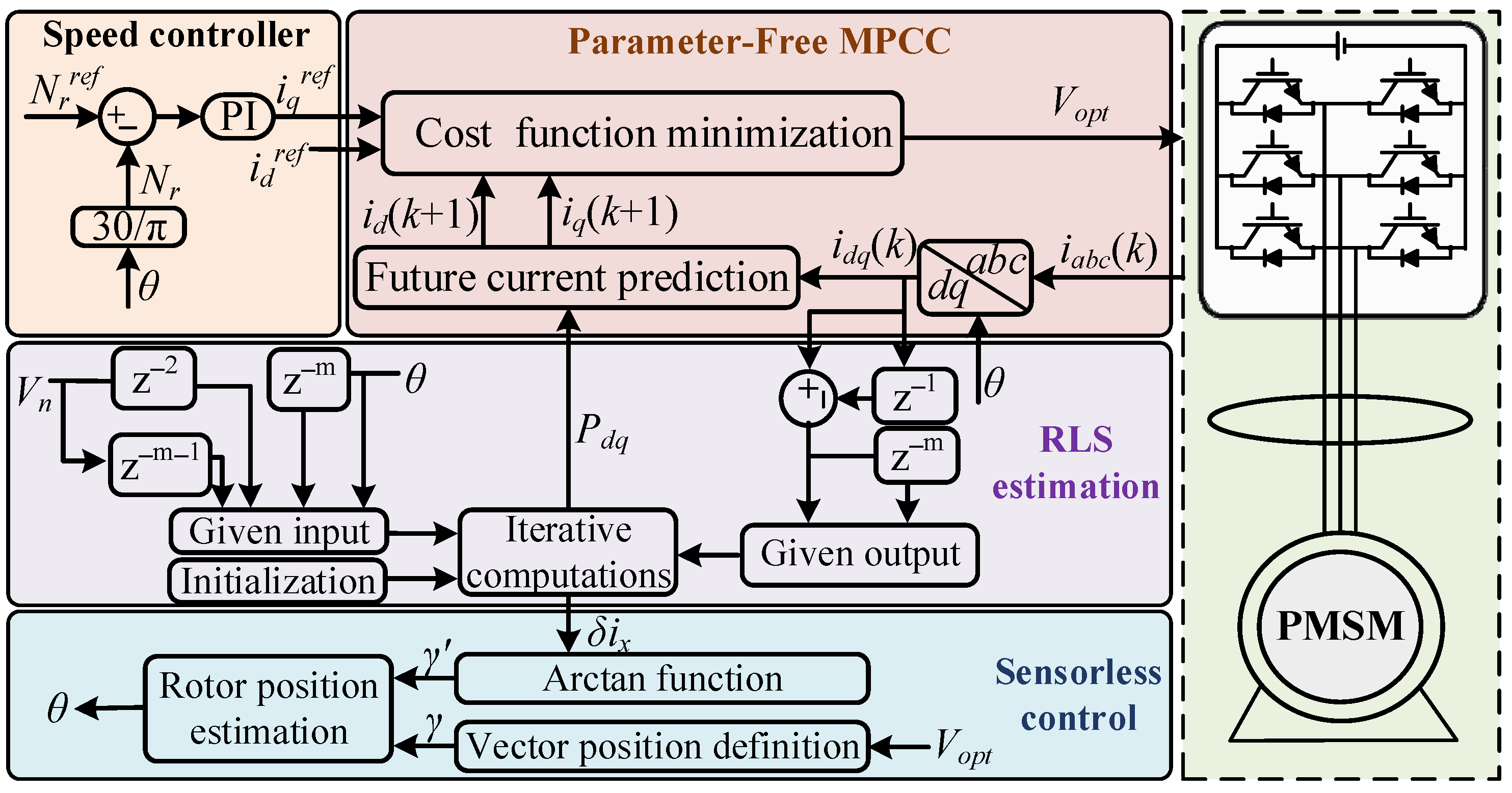
  • Collection and storage of the phase currents and applied voltage vectors and obtention of Ψx(x = d,q) and yx according to (15) and (16). Also, current reference iqref(k + 1) needs to be achieved through the speed controller.
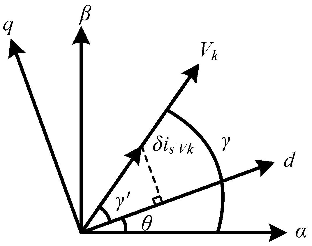
  • Relying on the applied voltage vector at (k − 1)th, vector position angle γ can be decided. Meanwhile, the angle between the voltage vector and the d-axis of the rotating coordinate system, namely γ′, needs to be achieved via the forced response of current variations through (26). Then, the rotor position angle θ can be estimated by (27).
  • The current variations need to be estimated through the RLS based on (23) and (24). Then, the future current can be predicted by (25).
  • The cost function gj (10) can be evaluated and the optimal voltage vector corresponding to the minimal gj needs to be selected to drive the inverter.
We also added the comparison results between the proposed and known strategies in Table 2.

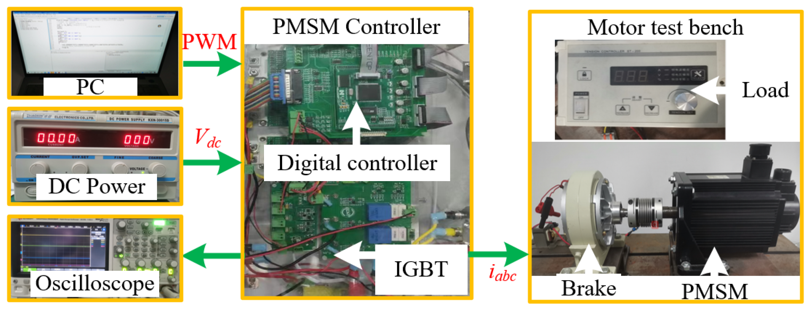
4. Experimental Results

To verify the effectiveness of proposed sensorless control strategy, this paper concerns a 1.2 kW prototype for the experiment, as presented in Figure 5. The whole hardware controller consists of the signal sampling module, the auxiliary power module, the PWM signal processing module and the minimum system board. Phase currents are measured by current sensor HAS50-S; then, current variation can be obtained. The master chip in the digital controller is TMS320F28335, and the three-phase inverter applies FF300R12ME4 IGBT modules. The sampling frequency is set as 10 kHz, and the motor parameters are all listed in Table 3.
In the case of parameter matching, the position estimation accuracy of the proposed control strategy is compared with that of traditional high-frequency injection position-free algorithm, in the speed commands of 50 rpm and 500 rpm, respectively. Figure 6 and Figure 7 present the actual and estimated values, where the superscript “est” denotes estimated value. It can be seen that the estimated speed of the two sensorless control strategies is basically consistent with the actual speed, ensuring the accuracy of speed information. However, the traditional control technique has larger location estimate mistakes and more fluctuating speed because digital filters inherently have issues throughout the signal extraction process, such as signal amplitude attenuation, phase delay, and complex parameter tuning. In general, the proposed strategy has more accurate position estimation.
To verify the robustness against parameter variations, the contrast experiments are carried out between proposed parameter-free control and model-free control in [23], when the model is mismatched and the speed command is 300 rpm. Obviously, both control strategies can maintain good sinusoidal phase current and stable rotational speed as presented in Figure 8. To be specific, the dq-axes prediction error of the control strategy based on RLS is basically guaranteed to be less than 0.2, while that of the control strategy based on the current variation lookup table is basically around 0.4. Thus, the future current state prediction under the proposed strategy is more accurate and the q-axis current ripple is smaller.
Figure 9 further shows the contrastive steady-state results of the phase current, the torque and the d-axis current when the speed command is 100 rpm. Apparently, the phase currents are almost sinusoidal in two strategies. However, the model-free control in [23] fails to completely avoid the problem of stagnation of current variation update, so that it is difficult to keep the predicted current consistent with the actual current, yielding a large prediction error. Instead, the predicted current error is significantly reduced in the proposed control strategy based on the reliable estimated current variations through RLS. In general, the proposed parameter-free control strategy based on RLS reduces the influence of rotor position estimation error to some extent.
To verify the satisfactory dynamic performance of the proposed control strategy, the experiments are carried out with variable speed and torque. Figure 10 provides the comparison results of position estimation accuracy between proposed control strategy and traditional high-frequency injection method under an accelerating condition. When the speed reference is increased from 200 rpm to 500 rpm, both control strategies exhibit similar dynamic response times. However, the position estimation error in the proposed control strategy, relying on forced response value estimation, is obviously reduced, particularly during sudden speed changes. Similarly, the comparison results of rotor position estimation are presented in Figure 11, where the load command is increased from 1 N∙m to 8 N∙m. It can be observed that the estimated position angle can precisely track actual values in the proposed control strategy, whereas the traditional high-frequency injection method results in noticeable discrepancies. There is no denying that the proposed control strategy performs satisfactorily under dynamic operating conditions.

5. Conclusions

On the basis of RLS, a parameter-free MPCC control is applied for PMSM where the rotor position is obtained without any sensors. This strategy is appropriate for limited volume systems and time-varying work conditions. To be specific, the future current is no longer predicted by the mathematical model of the motor, but the estimated current variations. In addition, the relationship between the forced response and the active voltage vector in the current variation is fully utilized to obtain the rotor position. The experimental results show that the proposed control strategy can still accurately estimate the rotor position in the case of low and mutational speed command, and the estimation errors of rotor position are reduced to around 0.1 rad lower than that in [14]. When the parameters are mismatched, the proposed strategy has significantly better parameter robustness compared with that of the traditional sensorless control strategy. Simultaneously, the proposed strategy estimates the natural attenuation and the forced response by RLS in each cycle, avoiding the problem of stagnant current variation update in [23]. In general, such sensorless parameter-free MPCC broadens the application range of the PMSM. Considering the limitation of input data in RLS, in the future, we will conduct a further study to get rid of RLS algorithms so that the system can become more stable.

Author Contributions

Conceptualization, L.L. and F.Y.; methodology, L.L. and F.Y.; software, F.Y. and L.R.; validation, L.L. and F.Y.; formal analysis, L.L. and F.Y.; investigation, C.L. and F.Y.; resources, L.R. and C.L.; data curation, L.R. and C.L.; writing—original draft preparation, L.R. and C.L.; writing—review and editing, L.L. and F.Y.; visualization, L.R.; supervision, C.L. and L.R.; project administration, C.L.; All authors have read and agreed to the published version of the manuscript.

Funding

This research was funded by Natural Science Foundation of the Jiangsu Higher Education Institutions of China, grant number 22KJB470025, and Natural Science Foundation of Jiangsu Province, grant number BK20210837.

Data Availability Statement

Not applicable.

Conflicts of Interest

The authors declare no conflict of interest.

References

  1. Hong, D.K.; Hwang, W.; Lee, J.Y.; Woo, B.C. Design, Analysis, and Experimental Validation of a Permanent Magnet Synchronous Motor for Articulated Robot Applications. IEEE Trans. Magn. 2018, 54, 8201304. [Google Scholar] [CrossRef]
  2. Li, X.; Xue, Z.; Yan, X.; Zhang, L.; Ma, W.; Hua, W. Low-Complexity Multivector-Based Model Predictive Torque Control for PMSM with Voltage Preselection. IEEE Trans. Power Electron. 2021, 36, 11726–11738. [Google Scholar] [CrossRef]
  3. Huang, W.; Hua, W.; Yin, F. Model Predictive Thrust Force Control of a Linear Flux-Switching Permanent Magnet Machine with Voltage Vectors Selection and Synthesis. IEEE Trans. Ind. Electron. 2019, 66, 4956–4967. [Google Scholar] [CrossRef]
  4. Wang, W.; Liu, C.; Liu, S.; Zhao, H. Model Predictive Torque Control for Dual Three-Phase PMSMs with Simplified Deadbeat Solution and Discrete Space-Vector Modulation. IEEE Trans. Energy Convers. 2021, 36, 1491–1499. [Google Scholar] [CrossRef]
  5. Zhang, X.; Li, J. Model Predictive Switching Control for PMSM Drives. IEEE J. Emerg. Sel. Topics Power Electron. 2023, 11, 942–951. [Google Scholar] [CrossRef]
  6. Yu, F.; Li, K.; Zhu, Z.; Liu, X. An Over-Modulated Model Predictive Current Control for Permanent Magnet Synchronous Motors. IEEE Access 2022, 10, 40391–40401. [Google Scholar] [CrossRef]
  7. Im, J.; Kim, R. Improved Saliency-Based Position Sensorless Control of Interior Permanent-Magnet Synchronous Machines with Single DC-Link Current Sensor Using Current Prediction Method. IEEE Trans. Ind. Electron. 2018, 65, 5335–5343. [Google Scholar] [CrossRef]
  8. Tang, Q.; Shen, A.; Luo, P. IPMSMs Sensorless MTPA Control Based on Virtual q-Axis Inductance by Using Virtual High-Frequency Signal Injection. IEEE Trans. Ind. Electron. 2020, 67, 136–146. [Google Scholar] [CrossRef]
  9. Xiao, D.; Nalakath, S.; Filho, S. Universal Full-Speed Sensorless Control Scheme for Interior Permanent Magnet Synchronous Motors. IEEE Trans. Power Electron. 2021, 36, 4723–4737. [Google Scholar] [CrossRef]
  10. Teymoori, V.; Kamper, M.; Wang, R.-J.; Kennel, R. Sensorless Control of Dual Three-Phase Permanent Magnet Synchronous Machines—A Review. Energies 2023, 16, 1326. [Google Scholar] [CrossRef]
  11. Fadi, A.; Ahmad, A.; Rabia, S.; Cristina, M.; Ibrahim, K. Velocity Sensor Fault-Tolerant Controller for Induction Machine using Intelligent Voting Algorithm. Energies 2022, 15, 3084. [Google Scholar]
  12. Jiang, Y.; Xu, W.; Mu, C.; Zhu, J.; Dian, R. An Improved Third-Order Generalized Integral Flux Observer for Sensorless Drive of PMSMs. IEEE Trans. Ind. Electron. 2019, 66, 9149–9160. [Google Scholar] [CrossRef]
  13. Chen, S.; Ding, W.; Wu, X.; Huo, L.; Hu, R.; Shi, S. Sensorless Control of IPMSM Drives Using High-Frequency Pulse Voltage Injection with Random Pulse Sequence for Audible Noise Reduction. IEEE Trans. Power Electron. 2023, 38, 9395–9408. [Google Scholar] [CrossRef]
  14. Wang, G.; Yang, L.; Yuan, B.; Wang, B.; Zhang, G.; Xu, D. Pseudo-Random High-Frequency Square-Wave Voltage Injection Based Sensorless Control of IPMSM Drives for Audible Noise Reduction. IEEE Trans. Ind. Electron. 2016, 63, 7423–7433. [Google Scholar] [CrossRef]
  15. Gao, S.; Yuan, L.; Dai, Y.; Mou, D.; Chen, K.; Zhao, Z. High-Frequency Current Predictive Control Method for Multiactive-Bridge Converter. IEEE Trans. Power Electron. 2022, 37, 10144–10148. [Google Scholar] [CrossRef]
  16. Yang, H.; Zhang, Y.; Walker, P.D.; Liang, J.; Zhang, N.; Xia, B. Speed Sensorless Model Predictive Current Control with Ability to Start a Free Running Induction Motor. IET Electr. Power Appl. 2017, 11, 893–901. [Google Scholar] [CrossRef]
  17. Kumar, P.; Bhaskar, D.V.; Muduli, U.R.; Beig, A.R.; Behera, R.K. Iron-Loss Modeling with Sensorless Predictive Control of PMBLDC Motor Drive for Electric Vehicle Application. IEEE Trans. Transp. Electr. 2021, 7, 1506–1515. [Google Scholar] [CrossRef]
  18. Liu, K.; Wang, X.; Wang, R.; Sun, G.; Wang, X. Antisaturation Finite-Time Attitude Tracking Control Based Observer for a Quadrotor. IEEE Trans. Circuits-II 2021, 68, 2047–2051. [Google Scholar] [CrossRef]
  19. Liu, J.; Cao, J.; Li, L. A Novel Method for Estimating the Position and Speed of a Winding Segmented Permanent Magnet Linear Motor. Energies 2023, 16, 3361. [Google Scholar] [CrossRef]
  20. Wang, H.; Wu, T.; Guo, Y.; Lei, G.; Wang, X. Predictive Current Control of Sensorless Linear Permanent Magnet Synchronous Motor. Energies 2023, 16, 628. [Google Scholar] [CrossRef]
  21. Eid, M.A.E.; Elbaset, A.A.; Ibrahim, H.A.; Abdelwahab, S.A.M. Modelling, Simulation of MPPT Using Perturb and Observe and Incremental Conductance techniques For Stand-Alone PV Systems. In Proceedings of the 2019 21st International Middle East Power Systems Conference (MEPCON), Cairo, Egypt, 17–19 December 2019; pp. 429–434. [Google Scholar]
  22. Eid, M.A.E.; Abdelwahab, S.A.M.; Ibrahim, H.A.; Alaboudy, A.H.K. Improving the Resiliency of a PV Standalone System under Variable Solar Radiation and Load Profile. In Proceedings of the 2018 Twentieth International Middle East Power Systems Conference (MEPCON), Cairo, Egypt, 18–20 December 2018; pp. 570–576. [Google Scholar]
  23. Yu, F.; Zhou, C.; Liu, X.; Zhu, C. Model-Free Predictive Current Control for Three-Level Inverter-Fed IPMSM with an Improved Current Difference Updating Technique. IEEE Trans. Energy Convers. 2021, 36, 3334–3343. [Google Scholar] [CrossRef]
  24. Wu, X.; Zhu, Z.; Freire, N.M.A. High Frequency Signal Injection Sensorless Control of Finite-Control-Set Model Predictive Control with Deadbeat Solution. IEEE Trans. Ind. Appl. 2022, 58, 3685–3695. [Google Scholar] [CrossRef]
  25. Wei, Y.; Xie, H.; Ke, D.; Wang, F. Sensorless Model-Free Predictive Current Control with Variable Prediction Horizon by Estimated Position for PMSM. In Proceedings of the 2022 25th International Conference on Electrical Machines and Systems (ICEMS), Chiang Mai, Thailand, 29 November–2 December 2022; pp. 1–5. [Google Scholar]
  26. Zhu, X.; Zhang, L.; Xiao, X.; Lee, C.H.T.; Que, H. Adjustable-Flux Permanent Magnet Synchronous Motor Sensorless Drive System Based on Parameter-Sensitive Adaptive Online Decoupling Control Strategy. IEEE Trans. Transp. Electr. 2023, 9, 501–511. [Google Scholar] [CrossRef]
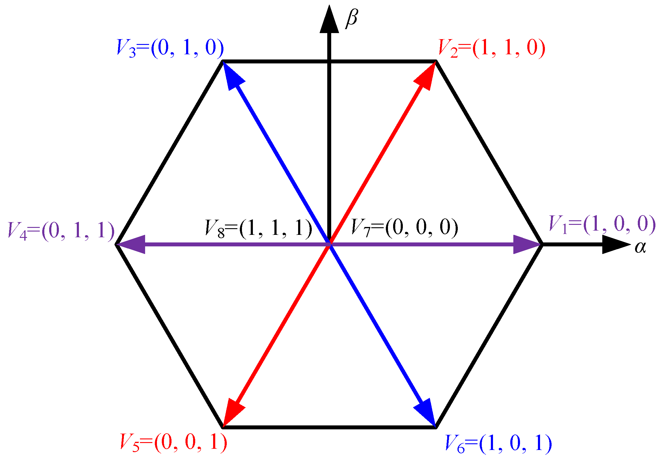
Figure 1. Space voltage vector distribution in a two-level inverter.
Energies 16 06792 g001
Figure 2. Schematic diagram of the stator current prediction based on once current detection.
Energies 16 06792 g002
Figure 3. Schematic diagram of rotor position estimation.
Energies 16 06792 g003
Figure 4. Structure of the proposed MPCC strategy.
Energies 16 06792 g004
Figure 5. Hardware experiment platform.
Energies 16 06792 g005
Figure 6. Comparative results between actual and estimated value at 50 rpm speed command. (a) Proposed control strategy. (b) Conventional sensorless control in [14].
Energies 16 06792 g006
Figure 7. Comparative results between actual and estimated value at 500 rpm speed command. (a) Proposed control strategy. (b) Conventional sensorless control in [14].
Energies 16 06792 g007
Figure 8. Experimental results of steady-state performance. (a) Proposed control strategy. (b) Parameter-free MPCC in [23].
Energies 16 06792 g008
Figure 9. Experimental results of steady-state performance. (a) Proposed control strategy. (b) Parameter-free MPCC in [23].
Energies 16 06792 g009
Figure 10. Experimental results of rotor position estimation when speed command changes. (a) Proposed control strategy. (b) Conventional sensorless control in [14].
Energies 16 06792 g010
Figure 11. Experimental results of rotor position estimation when load command changes. (a) Proposed control strategy. (b) Conventional sensorless control in [14].
Energies 16 06792 g011
Table 1. Voltage position definition.
Voltage VectorSabcVector Position Angle γVoltage VectorSabcVector Position Angle γ
V11000V2110π/3
V30102π/3V4011π
V50014π/3V61015π/3
V70000V81110
Table 2. Comparison between the proposed and known strategies.
Reference[14][17][18][26]Proposed
Requires gain tuningNoYesYesYesNo
Estimation errorsMiddleLowLowMiddleLow
Parameter robustnessLowLowLowHighHigh
Relative Simplicity of algorithmLowHighMiddleMiddleMiddle
Table 3. Motor parameters.
ParametersValues
Rated power1.2 kW
Rated voltage380 V
Rated current5 A
Rated torque8 N∙m
Rated speed1500 rpm
Inductance of direct axis24 mH
Inductance of quadrature axis36 mH
Stator resistance5.25 Ω
Moment of inertia0.001 kg·m2
Pole pairs2
Permanent magnet flux linkage0.8 Wb
Disclaimer/Publisher’s Note: The statements, opinions and data contained in all publications are solely those of the individual author(s) and contributor(s) and not of MDPI and/or the editor(s). MDPI and/or the editor(s) disclaim responsibility for any injury to people or property resulting from any ideas, methods, instructions or products referred to in the content.

