Abstract
Lithium-ion batteries are a key technology for the electrification of the transport sector and the corresponding move to renewable energy. It is vital to determine the condition of lithium-ion batteries at all times to optimize their operation. Because of the various loading conditions these batteries are subjected to and the complex structure of the electrochemical systems, it is not possible to directly measure their condition, including their state of charge. Instead, battery models are used to emulate their behavior. Data-driven models have become of increasing interest because they demonstrate high levels of accuracy with less development time; however, they are highly dependent on their database. To overcome this problem, in this paper, the use of a data augmentation method to improve the training of artificial neural networks is analyzed. A linear regression model, as well as a multilayer perceptron and a convolutional neural network, are trained with different amounts of artificial data to estimate the state of charge of a battery cell. All models are tested on real data to examine the applicability of the models in a real application. The lowest test error is obtained for the convolutional neural network, with a mean absolute error of 0.27%. The results highlight the potential of data-driven models and the potential to improve the training of these models using artificial data.
1. Introduction
As the transportation sector is responsible for a large share of greenhouse gas emissions, it is crucial for the automotive and mobility industry to turn towards renewable energy []. Lithium-ion batteries (LIBs) have taken a predominant role as electrochemical energy storage solutions in many applications, ranging from portable consumer electronics to integration in power grids and battery electric vehicles (BEVs) []. Next to applications in stationary energy storage systems with particularly high efficiency needs in third-world countries [], LIBs are best-suited for empowering BEVs due to their high energy densities and their long lifespans []. Nevertheless, the operation of LIBs has to be optimized to exceed the performance of internal combustion engine vehicles. The demand for BEVs is growing quickly, and the materials they require are rare. The optimization of BEVs is essential for their worldwide success, especially in developing countries, such as Latin American countries, which have large populations and uncertain future markets []. The whole lifecycle of the BEV, including production, operation, recycling, and reuse, has to be considered. Additionally, the price pressure seen regarding BEVs intensifies the need for further enhancements during operation []. The battery management system (BMS) of a BEV is responsible for determining the condition of the vehicle’s battery. This system monitors and controls the battery cells []. During operation, the condition of a battery is influenced by various intertwined parameters and the ambient conditions []. Additionally, there are several mechanisms for the degradation of an LIB, all of which directly affect the performance and the state of the battery. These mechanisms are caused by chemical processes, mechanical damage, temperature, and different loading conditions [].
A key challenge for the application of LIBs is to accurately predict their state of charge (SoC), which is necessary to ensure their safety and facilitate their efficient charge and discharge cycles []. Other than physical estimation methods, such as coulomb counting or other electrochemical models [,,], there are primarily two different approaches: model-based approaches and data-driven approaches. The main representatives of the model-based methods are from the Kalman filter family, including the extended Kalman filter, dual extended Kalman filter, and unscented Kalman filter models [,,]. The data-driven methods utilize machine learning (ML) or other statistical algorithms to estimate the condition of a battery. Because these algorithms approximate the electrochemical processes inside a battery cell with high levels of accuracy while having decreased levels of complexity, they have gained considerable interest []. The main reason for the success of a data-driven method is the data the method is based on, which should be reliable and capture the behavior of the cell []. Poor data impede the state estimation for batteries, as the parameters are highly dependent on the loading as well as the ambient conditions and are further internally correlated []. The methods used to estimate the SoC of a battery include support vector machines (SVM) [], regression algorithms [], and artificial neural networks (ANNs) []. Different types of ANNs can be distinguished from one another. The conventional type are multilayer perceptrons (MLP), which are feedforward neural networks []. The other applied types are recurrent neural networks (RNNs) [,] and convolutional neural networks (CNNs), where the convolution is typically performed along the time axis [,]. The aim of the data-driven models is to approximate a function between the measurable parameters of a battery and the nonmeasurable conditions, such as the SoC. As ML models are highly dependent on their input data, it is crucial to have a sufficiently large dataset to replicate the behavior of a battery. For LIBs in particular, which have several working conditions and respond differently to changing ambient conditions, creating an appropriate dataset is a key challenge. Furthermore, battery tests are time- and cost-consuming []. A possible solution to overcome these problems is the usage of artificially augmented data. In the last few years, it has been shown that data augmentation techniques can lead to improved results for ML models, thus making it possible to successfully tackle the problem of limited datasets [,,].
In this work, the SoC of an LIB is estimated using different ML algorithms. To decrease the effort required for time-consuming battery tests to a minimum, a real-world dataset is enriched using artificially augmented data. The goal is to approximate a function for the SoC with the current, voltage, and temperature as input variables. After preprocessing, the data are used to train and test the ML models. The results are compared to a reference model, which is a linear regression model. Two types of ANNs, an MLP and a CNN, are trained and tested to evaluate the impact of the data augmentation technique. The MLP is chosen because of its lower complexity and simpler structure in comparison with other ANNs. Therefore, less computing power is needed to train the model. An advantage of CNNs is their additional data processing step along the time axis, which allows the accuracy of the model to benefit from determining more complex correlations, which are not identifiable using only the rare input data.
2. Materials and Methods
2.1. Data Origin and Data Augmentation
The parameters of a battery are highly intercorrelated. During operation, it is important to accurately monitor the condition of the cells to ensure efficient usage and adequate loading. In the process of developing an ML model, considerable attention must be paid to the selection of features, as the results are highly dependent on the input data. The data processing steps include data collection, data cleaning, and data transformation []. Real-world data were obtained by loading an LIB in a battery test system. The experiments were conducted using the Molicel 21700 P42a battery cell, which has a capacity of 4.2 Ah with an end-of-charge voltage of 4.2 V ± 0.05 and a cut-off voltage of 2.5 V. The battery was cycled in a temperature chamber at a constant temperature of 23 °C. The test system was an OctoStat5000 from Ivium Technologies. The cell was discharged in ten percent intervals from a SoC of 100% to a SoC of 0%. Every 0.5 s, the voltage, current, and temperature of the cell were measured. A discharge cycle of the analyzed battery cell is shown in Figure 1.
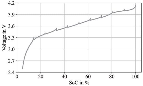
Figure 1.
Discharge cycle of the analyzed battery cell with voltage plotted over the SoC. The cell is discharged in 10% intervals and rested after each interval.
Based on the real-world data, a data augmentation technique is applied to enrich the data basis for training the ML models. The input data for the algorithms, also called features, are current, temperature, and voltage. The output of the models, referred to as target value, is the SoC. To artificially create the new data, a whole discharge cycle is used and the current as well as the SoC values are kept constant. Two different regression models are trained for voltage and temperature, using a ridge regression. The loss function L, consisting of the squared error between observed y and predicted values y*, is supplemented by an L2-penalty for the weight parameters w to decrease the risk of overfitting and to process the highly correlated data. This is summarized in (1).
Based on the previous ten time steps, which is equivalent to five seconds cumulated with a sample rate of 0.5 s, the next value for voltage, respectively, temperature, is estimated. Both models are regression algorithms and, therefore, can be demonstrated in a regression formula. The regression equation for the voltage estimation is shown in (2), and for the temperature in (3). The target value is the current value of timestep t for voltage and temperature, respectively.
To keep the computation time and the processing power low, only every twentieth measurement point is calculated using the regression model. The data points between these reference points are interpolated. At first, the estimation models for voltage and temperature are tested against real measurements to validate their accuracy. Even though these models are highly accurate, a small error benefits the data augmentation as further randomness is included in the process. Following that, the real input data are slightly modified. Therefore, new reference points are estimated, and a new discharge curve is created. Again, the data between the reference points are interpolated. Demonstrated in Figure 2, the accuracy and two artificially created discharge curves are shown as an example for the voltage.
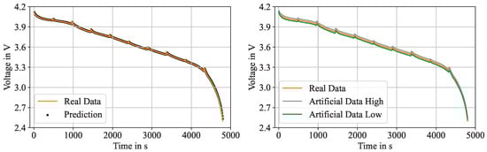
Figure 2.
Results of the data augmentation method. On the left, the accuracy of the voltage estimation model for real data is presented. Real measurements are compared to the results of the voltage estimation model. On the right, results of the estimation model with slightly modified input values resulting in two artificially created discharge curves are shown.
Before the data are used in the ML models, they are preprocessed. At first, the data are normalized by using a standard scaler. By means of the mean values and the standard deviation , the data are transformed, resulting in a data distribution with zero mean and unit variance []. This is performed for each battery parameter.
In a crucial step for the high performance of ML models []), the dimension of the data is reduced after the normalization, which can be referred to as the actual feature selection. In context of the curse of dimensionality and to reduce the risk of overfitting, a principal component analysis (PCA) is conducted. In sum, the curse of dimensionality describes the problem of an exponentially growing search space with an increasing amount of features []. A PCA is a method to reduce the dimension of a problem by analyzing the variance of the data [], which is transformed into a new coordinate space with a lower dimension. This is especially useful while working with highly intercorrelated data []. The principal components are orthonormal axes, which cover a certain value of variance of the initial data. These components are given by the dominant eigenvectors of the sample covariance matrix. They can be identified by the largest corresponding eigenvalues []. The PCA is connected to the singular value decomposition (SVD), which is a matrix factorization that can also be used to reduce the dimension. A SVD is typically computationally more efficient, and because of the relation between the singular and the eigenvalues, the SVD in (4) can be used to calculate the principal components. M is the feature matrix, V is the orthonormal basis of the eigenvectors of , ∑ is a diagonal matrix with the singular values , which are the square roots of the eigenvalues , and U is the orthonormal matrix, which can be calculated using (5) [].
After preprocessing the data, the features are used to train different ML models. The training data consist of 80% of the initial data plus the augmented data, and the test data make up the remaining 20%. These models are introduced in the following.
2.2. Machine Learning Models
2.2.1. Linear Regression
As a reference model, and to compare the results to a less complex model, a linear regression is implemented. Based on weight parameters , which are determined during the training, a linear function between the input features voltage, current, and temperature, as well as the target values, is approximated. The estimated values y* are calculated using (6) [].
By minimizing the squared error between the real and predicted values, the values for the weight parameters are determined. The corresponding loss function L is shown in (7).
The reference model is an ordinary least square approach to determine the SoC based on measurement values of voltage, current, and temperature.
2.2.2. Artificial Neural Networks
Two types of ANNs are used to predict the SoC. The first one is an MLP, which is a simple feedforward neural network. All neurons from a layer are connected to the neurons from the next layer. The information is passed on in one direction to the output layer, where the target value is calculated. The inputs in a neuron are summed up and are then further processed in an activation function, where the output is calculated. The chain of mathematical functions is used to approximate the target values. To determine the appropriate parameters of the model, a four-fold-cross-validation was conducted by dividing the training data into four equally sized groups. One group acts as the validation set and the remaining groups as training data []. There are approaches in the literature using an MLP to estimate the SoC of a battery cell []. The structure of applied feedforward neural networks in the area of SoC estimation is mainly kept simple, with only a few hidden layers and a low number of neurons [,,]. The structure of the proposed MLP consists of three hidden layers with ten neurons in both the first and the second hidden layer and five neurons in the third hidden layer. As activation function, the rectified linear unit (ReLU) function is used, which has another advantage of efficient model training. The final learning rate is 0.1 and the Adam optimizer is used to improve the training speed and ensure the accuracy of the estimation results [].
The second applied model is a CNN. While the main application of CNNs is image processing, it is gaining more and more interest for other areas as well [,]. The first approaches to estimate the condition of a battery cell can be found in the literature. Most of the CNN-based models are used in combination with other ANNs [,]. The main difference for an MLP is the convolution by means of a kernel function. When analyzing time series data, the convolution is conducted along the time axis []. Typically, the kernel filter is followed by a pooling layer, where several points can be pooled in a single data point []. Instead of an MLP, where the neurons are fully connected, CNNs reduce and reassemble the feature matrix to learn new and complex patterns of the input data. The structure and the general approach of a CNN is shown in Figure 3 [].
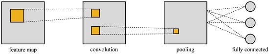
Figure 3.
Structure of a CNN with a feature map followed by a convolution, a pooling layer, and a fully connected layer. The filter is moved across the features.
The applied CNN consists of two convolution layers with a pooling layer followed by another two convolutions and a pooling layer. During the convolution, 32 randomly initialized filters are used in the first part and 16 filters are used in the second part. When applying the filters, the window size is five timesteps along the temporal axis and the dimension is not affected during the convolution. The final layer is a fully connected layer, where the value for the SoC is estimated. As a metric during the training of the model, the coefficient of determination is used, which is shown in (8). The score is calculated by means of the real values , the predicted values , and the mean value .
3. Results
Three different ML models are trained, respectively, with and without data augmentation to evaluate the accuracy of the SoC prediction. The raw data are temperature, voltage, and current values. The test data are exclusively real data. To have a benchmark and a comparison for the neural networks, a linear regression model is used as reference. The input data in all models are the same. To analyze the impact of the data augmentation technique, the results are calculated without artificial data, with ten times the initial data, and with 20 times the initial data. All models are retrained five times and the mean values as well as the standard deviation are presented, as the initialization of the data augmentation technique and the neural networks is random and therefore slightly different. The results for the linear regression are shown in Table 1. The MAE and the RMSE are separated for the training and the test of the models. All mean values and the corresponding standard deviation are listed for the three different input datasets.

Table 1.
Results of the linear regression with the three different sizes of training datasets. The mean of five times retraining the model and the corresponding standard deviations are shown.
The impact of the data augmentation method on the linear regression is small. In comparison to other ML algorithms, the dependence of a linear regression on a large database is slight, and an impact or a significant improvement was not expected. Accordingly, the results for all three different sizes of training data are similar and no influence of the data augmentation method can be measured. Nevertheless, it is possible to estimate the SoC with a simple linear model with error values below 5%. There is no overfitting and, consequently, the test errors are similar to the training errors. Nevertheless, the main focus of the linear model is to have reference accuracies for the neural networks.
Before analyzing the accuracies of both models, the convergence during the training of the models is examined. During the training, the weights are updated after each epoch. The training phase with the MAE over the epochs for the MLP is shown in Figure 4a and for the CNN in Figure 4b.
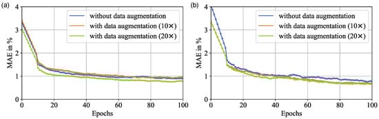
Figure 4.
Convergence of the different models. MAE is shown over the epochs for the MLP (a) and the CNN (b) with and without augmented data.
A comparison of the convergence is drawn between the performance with different input data for both models. The convergence for the model without augmented data is indicated in blue, with ten times the initial data in orange, and with 20 times the initial data in green. As expected, the error is decreasing quickly over the first epochs, and then converges against a certain value. This behavior can be determined for all input data, but there are differences in the number of epochs to reach the final value and the final error itself. For both models, the augmented data are favorable for convergence, as the error decreases faster than it does without the augmented data. The difference is greater for the MLP, but also visible for the CNN. A faster convergence has the advantages of less training effort and a higher robustness, as there is less chance to become stuck in a local minima. Although the difference in the convergence behavior is apparent, it is in a smaller range and is, therefore, not significant for the optimization of the model. Further, regardless of the training dataset, each model converges to a similar value. In comparison, the CNN drops faster below an MAE of 1%, and the differences between the model with and without augmented data are slightly greater. This can also be shown when analyzing the accuracies of each model. The first examined ANN is the MLP. The preprocessed input data are passed through the layers of the MLP and the SoC is estimated. The results are summarized in Table 2. Similar to Table 1, the MAE and RMSE with the corresponding standard deviations are shown for the training and test of both models with the same three different input datasets.
Table 2.
Results of the MLP with the three different sizes of training datasets. The mean of five times of retraining the model and the corresponding standard deviations are shown.
Firstly, it can be noted that the model shows significantly higher accuracies than the linear model. Even the test RMSE is below 1% for all three datasets. Despite this notion, the impact of the data augmentation technique is small. The errors of the dataset with ten times the initial data are lower, but they are increasing with a higher amount of data. The standard deviation is also not highly impacted. The general ability to estimate the SoC can be determined. Additionally, the PCA is working efficiently, as no indications for overfitting can be detected. Further optimization with data augmentation is not necessary. Even though it does not deteriorate the performance of the model, the influence on the error and the standard deviation is low. The dimension reduction method improves the ratio between dimension and number of features and, thus, the influence of the data augmentation method on the simpler neural network is low.
In comparison to that, a CNN is used to learn new and complex patterns in the input data. This is conducted by using a convolution filter along the time axis. The results are summarized in Table 3.
Table 3.
Results of the CNN with the three different sizes of training datasets. The mean of five times of retraining the model and the corresponding standard deviations are shown.
Several aspects are striking when analyzing the results of the CNN. Without the augmented data, the CNN is slightly worse than the MLP. Additionally, the difference between training and test errors is higher, which is an indicator that there is potential for optimization. Further, the standard deviation is higher. In comparison to the MLP, there is a higher degree of randomness, as the filters for the convolution are randomly initialized. The model learns complex patterns in the data, but is not able to reproduce them with the limited database. Still, the standard deviation is not high and acceptable, but the fluctuation of the CNN is higher. By increasing the amount of training data, the errors are decreasing. While using ten times the initial data, the training MAE could be reduced by over 50% from 0.975% to 0.371%. With 20 times the initial data, the error could again be decreased to 0.261%. Further, the standard deviation is also decreasing, which means that the patterns in the data can be learned regardless of the filters. The filters vary while retraining the model. With a sufficiently large dataset, the impact of the filters and the uncertainty of the model is decreasing. The same behavior can be shown for the test data. The difference between training and test errors is small and, therefore, there is no overfitting. On the contrary, some test errors are slightly lower than the training errors using augmented data. The reason for that is the data augmentation technique, which should reflect a wider range of discharge behavior. Consequently, there is a higher variety in the training dataset, which could lead to higher errors; yet, still, the errors are nearly the same. The direct comparison of the errors of MLP and CNN with the corresponding standard deviations is shown in Figure 5. The error bars displaying the MAE are demonstrated for the different input data and, further, the uncertainty for retraining the model is shown. While the impact on the MLP is small, the optimization potential using augmented data is clearly visible for the CNN.
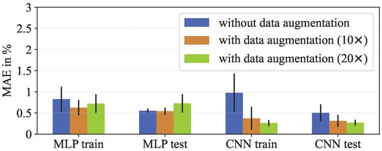
Figure 5.
Error bars and standard deviation of the five times retrained models without data augmentation, with ten times the initial data and 20 times the initial data. The MAE is shown for the MLP and the CNN.
As stated before, the test data consist of only real data of a discharge cycle. Therefore, a direct comparison between real data and the prediction of the model can be drawn. For the MLP, this is shown in Figure 6a and for the CNN in Figure 6b. For a full discharge cycle, the voltage is shown over the SoC. The real experimental data are indicated in gray. The results of the final model with augmented data are demonstrated in orange.
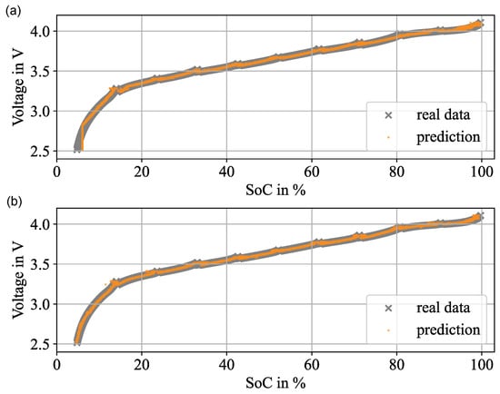
Figure 6.
Test results of the SoC estimation model in comparison with the real values for the MLP (a) and for the CNN (b). The results for the SoC are shown over the last voltage value for the estimation.
The estimations and the real data are mainly overlapping. The drawbacks of the MLP can be seen in the high and low SoC areas and in the transition area from linear to nonlinear, where there are higher fluctuations in the estimation results. In the mainly linear range between a SoC of 20% to 80%, the performance of both models is similar. The CNN shows fewer outliers and, especially, the low SoC area can be accurately approximated. This behavior can explain the differences between a test MAE of the MLP with 0.727% and the CNN with 0.270%. As the edge areas are critical for an accurate state estimation, the CNN shows better results and is more suitable.
Overall, the performance of the CNN is slightly better. The impact of the data augmentation method is huge in relative values, but small in absolute values, as both neural networks show high accuracies by estimating the SoC without further data processing.
4. Discussion
When it comes to LIBs, a major challenge for balanced and safe loading cycles is the accurate determination of the condition of a battery cell. In comparison with conventional modeling techniques, data-driven models require less development time and no electrochemical characterization. Nevertheless, they need a reliable and large enough data basis, which covers the behavior of the cell. Especially for battery cells, for which tests and experiments are time- and cost-intensive, this is a key problem. Data augmentation, which is usually used for image processing, is a method to overcome this challenge by artificially creating new training data. In this case, two time-series forecasting models for voltage and temperature are developed. The accuracy of both models is high, which is shown in Section 2.1, but, moreover, the small error is favorable because of the additional randomness of the results. Therefore, new grid points are estimated and a wider range of input values is covered. Simultaneously, the current and the SoC values are kept constant. This technique relies on creating a whole discharge cycle, but it can also be used to enrich certain SoC areas. Only grid points are estimated because of the computing time. As a compromise between computing costs and accuracy, only every twentieth point is estimated. The points in between are interpolated. This interpolation does not impair the estimation and is hence sufficient for the data augmentation method. At first, a linear model is developed to predict the SoC. The errors are mainly below 5%. Although it could be shown that it is possible to determine the SoC with a linear regression, the accuracies cannot compete with conventional methods. Nevertheless, it is a reference model and a starting point to evaluate the results of the ANNs. In an MLP, the information is processed from input to output layer and a function between the features and the target values is approximated. The data augmentation technique has low impact on the accuracy of the MLP. A reason for that is the preprocessing method. ML algorithms are prone to overfit, when the dimension is equal to or greater than the number of features. This is the case for a feature matrix , where j is equal or greater than i. By reducing the dimension using the PCA, the tendency to overfit could be reduced. This is sufficient for the MLP, and the impact of the approach to artificially create additional data is decreased. Further, the testing data cover a limited range of loading conditions. Hence, analyzing the test errors does not capture the full capabilities of the optimized model. On the contrary, the CNN can determine more complex patterns, in which a huge database is beneficial. When examining the results of the CNN, it becomes apparent that the data augmentation technique increases the accuracy of the CNN. Two other advantages can be observed. First, the model converges earlier with the artificial data. Even though the improvement is small, there is less chance to become stuck in local minima, and fewer iterations are needed to train the model. Second, the standard deviation is decreasing, which results in a more robust model and an improved ability to reproduce the results.
Overall, the CNN shows better results and more potential for optimization. As the different loading conditions and their combinations are infinite in a real application, the ability to capture complex patterns in the input data is a key advantage of the CNN. The data augmentation method leads to improved results and the impact is expected to be higher for testing against several loading conditions. Still, the potential of data augmentation for the optimization of ANNs is evident. Further, the errors below 0.5% show that the CNN is able to accurately estimate the SoC. In comparison to conventional estimation models, such as representatives of the Kalman filter family, the errors could be slightly reduced [,,]. Next to that, there is no need for an elaborately electrochemical characterization of the cell. This shows the huge potential to determine the condition of a battery cell with data-driven methods.
5. Conclusions
The electrification of the transport sector is inevitable to reach environmental goals. LIBs as electrochemical energy storage systems are a crucial factor for the success of electric vehicles. For efficient and optimized driving cycles, it is important to be able to determine the condition of the battery at all times. As ML algorithms reach high accuracies, are robust, and need less development and computing time, they are a promising alternative to conventional battery models. Nevertheless, they need a reliable and huge dataset to represent reality; however, battery tests are time- and cost-consuming. Therefore, the applicability of data augmentation was examined in this paper to optimize the ML models. The data of real-world experiments with the battery cell Molicel 21700 P42a were used. The training data were enriched by artificially created data by means of linear estimation models for voltage and temperature, and the impact on the ML models was analyzed.
The additional data improve the performance of the models in terms of convergence, robustness, and accuracy. Both neural networks succeed the linear model and are able to estimate the SoC with errors below 1%. The linear model serves as a reference model, but the final results with error values around 4% to 5% cannot compete with the ANNs. Comparing both ANNs, the CNN reaches the lower test error with an MAE of 0.27% and outperforms the MLP with an MAE of 0.539%. Therefore, the CNN is identified as the most suitable model. Further, the optimization methods have a higher impact on the CNN. By means of the data augmentation method, it is possible to nearly halve the test error from 0.505% to the lowest error of 0.27%. Thus, the data augmentation method shows itself as an effective way to optimize the estimation model.
In the future, it is planned to further develop the data augmentation technique. The current method consists of linear estimations for grid points. The values between the grid points are interpolated. It should be examined if the estimations can be improved using other approaches while keeping the computing time and efforts low. Further, the proposed algorithm should be tested against a higher variety of loading conditions to evaluate possible fields of application and to compete with traditional estimation approaches.
Author Contributions
Conceptualization, S.P.; methodology, S.P.; software, S.P.; validation, S.P. and A.N.; formal analysis, S.P. and A.N.; investigation, S.P.; resources, S.P. and A.M.; data curation, A.M.; writing—original draft preparation, S.P.; writing—review and editing, S.P., A.M., M.K., A.N. and T.W.; visualization, S.P.; supervision, M.K., A.N. and T.W.; project administration, M.K., A.N. and T.W.; funding acquisition, M.K., A.N. and T.W. All authors have read and agreed to the published version of the manuscript.
Funding
This research [project MORE] is funded by dtec.bw—Digitalization and Technology Research Center of the Bundeswehr, which we gratefully acknowledge. dtec.bw is funded by the European Union—NextGenerationEU. Further, we acknowledge financial support by the University of the Bundeswehr Munich.
Data Availability Statement
The data presented in this study are available on request from the corresponding author.
Conflicts of Interest
The authors declare no conflict of interest.
Abbreviations
The following abbreviations are used in this manuscript:
| ANN | Artificial neural network |
| BEV | Battery electric vehicle |
| BMS | Battery management system |
| CNN | Convolutional neural network |
| LIB | Lithium-ion battery |
| MAE | Mean absolute error |
| ML | Machine learning |
| MLP | Multilayer perceptron |
| PCA | Principal component analysis |
| RMSE | Root mean square error |
| RNN | Recurrent neural network |
| SoC | State-of-Charge |
| SVD | Singular value decomposition |
| SVM | Support vector machine |
References
- Buberger, J.; Kersten, A.; Kuder, M.; Eckerle, R.; Weyh, T.; Thiringer, T. Total CO2-equivalent life-cycle emissions from commercially available passenger cars. Renew. Sustain. Energy Rev. 2022, 159, 112158. [Google Scholar] [CrossRef]
- Bernhart, W. Challenges and Opportunities in Lithium-ion Battery Supply. In Future Lithium-Ion Batteries; The Royal Society of Chemistry: London, UK, 2019; pp. 316–334. [Google Scholar] [CrossRef]
- Schulte, J.; Figgener, J.; Woerner, P.; Broering, H.; Sauer, D.U. Forecast-based charging strategy to prolong the lifetime of lithium-ion batteries in standalone PV battery systems in Sub-Saharan Africa. Sol. Energy 2023, 258, 130–142. [Google Scholar] [CrossRef]
- Stock, S.; Pohlmann, S.; Günter, F.J.; Hille, L.; Hagemeister, J.; Reinhart, G. Early Quality Classification and Prediction of Battery Cycle Life in Production Using Machine Learning. J. Energy Storage 2022, 50, 104144. [Google Scholar] [CrossRef]
- Castro, F.D.; Cutaia, L.; Vaccari, M. End-of-life automotive lithium-ion batteries (LIBs) in Brazil: Prediction of flows and revenues by 2030. Resour. Conserv. Recycl. 2021, 169, 105522. [Google Scholar] [CrossRef]
- Boxall, N.J.; King, S.; Cheng, K.Y.; Gumulya, Y.; Bruckard, W.; Kaksonen, A.H. Urban mining of lithium-ion batteries in Australia: Current state and future trends. Miner. Eng. 2018, 128, 45–55. [Google Scholar] [CrossRef]
- Wang, Y.; Tian, J.; Sun, Z.; Wang, L.; Xu, R.; Li, M.; Chen, Z. A comprehensive review of battery modeling and state estimation approaches for advanced battery management systems. Renew. Sustain. Energy Rev. 2020, 131, 110015. [Google Scholar] [CrossRef]
- Lee, J.H.; Lee, I.S. Lithium Battery SOH Monitoring and an SOC Estimation Algorithm Based on the SOH Result. Energies 2021, 14, 4506. [Google Scholar] [CrossRef]
- Shchurov, N.I.; Dedov, S.I.; Malozyomov, B.V.; Shtang, A.A.; Martyushev, N.V.; Klyuev, R.V.; Andriashin, S.N. Degradation of Lithium-Ion Batteries in an Electric Transport Complex. Energies 2021, 14, 8072. [Google Scholar] [CrossRef]
- Bonfitto, A. A Method for the Combined Estimation of Battery State of Charge and State of Health Based on Artificial Neural Networks. Energies 2020, 13, 2548. [Google Scholar] [CrossRef]
- Ng, K.S.; Moo, C.S.; Chen, Y.P.; Hsieh, Y.C. Enhanced coulomb counting method for estimating state-of-charge and state-of-health of lithium-ion batteries. Appl. Energy 2009, 86, 1506–1511. [Google Scholar] [CrossRef]
- Chaoui, H.; Mandalapu, S. Comparative Study of Online Open Circuit Voltage Estimation Techniques for State of Charge Estimation of Lithium-Ion Batteries. Batteries 2017, 3, 12. [Google Scholar] [CrossRef]
- Marcicki, J.; Canova, M.; Conlisk, A.T.; Rizzoni, G. Design and parametrization analysis of a reduced-order electrochemical model of graphite/LiFePO4 cells for SOC/SOH estimation. J. Power Sources 2013, 237, 310–324. [Google Scholar] [CrossRef]
- Hossain, M.; Haque, M.E.; Arif, M.T. Kalman filtering techniques for the online model parameters and state of charge estimation of the Li-ion batteries: A comparative analysis. J. Energy Storage 2022, 51, 104174. [Google Scholar] [CrossRef]
- Shrivastava, P.; Soon, T.K.; Idris, M.Y.I.B.; Mekhilef, S. Overview of model-based online state-of-charge estimation using Kalman filter family for lithium-ion batteries. Renew. Sustain. Energy Rev. 2019, 113, 109233. [Google Scholar] [CrossRef]
- Luo, Y.; Qi, P.; Kan, Y.; Huang, J.; Huang, H.; Luo, J.; Wang, J.; Wei, Y.; Xiao, R.; Zhao, S. State of charge estimation method based on the extended Kalman filter algorithm with consideration of time–varying battery parameters. Int. J. Energy Res. 2020, 44, 10538–10550. [Google Scholar] [CrossRef]
- Sharma, P.; Bora, B.J. A Review of Modern Machine Learning Techniques in the Prediction of Remaining Useful Life of Lithium-Ion Batteries. Batteries 2023, 9, 13. [Google Scholar] [CrossRef]
- Hannan, M.A.; Lipu, M.S.H.; Hussain, A.; Ker, P.J.; Mahlia, T.M.I.; Mansor, M.; Ayob, A.; Saad, M.H.; Dong, Z.Y. Toward Enhanced State of Charge Estimation of Lithium-ion Batteries Using Optimized Machine Learning Techniques. Sci. Rep. 2020, 10, 4687. [Google Scholar] [CrossRef]
- Basia, A.; Simeu-Abazi, Z.; Gascard, E.; Zwolinski, P. Review on State of Health estimation methodologies for lithium-ion batteries in the context of circular economy. CIRP J. Manuf. Sci. Technol. 2021, 32, 517–528. [Google Scholar] [CrossRef]
- Álvarez Antón, J.C.; García Nieto, P.J.; Blanco Viejo, C.; Vilán Vilán, J.A. Support Vector Machines Used to Estimate the Battery State of Charge. IEEE Trans. Power Electron. 2013, 28, 5919–5926. [Google Scholar] [CrossRef]
- Deng, Z.; Hu, X.; Lin, X.; Che, Y.; Xu, L.; Guo, W. Data-driven state of charge estimation for lithium-ion battery packs based on Gaussian process regression. Energy 2020, 205, 118000. [Google Scholar] [CrossRef]
- Cui, Z.; Wang, L.; Li, Q.; Wang, K. A comprehensive review on the state of charge estimation for lithium-ion battery based on neural network. Int. J. Energy Res. 2022, 46, 5423–5440. [Google Scholar] [CrossRef]
- Li, X.; Jiang, H.; Guo, S.; Xu, J.; Li, M.; Liu, X.; Zhang, X.; Bhardwaj, A. SOC Estimation of Lithium-Ion Battery for Electric Vehicle Based on Deep Multilayer Perceptron. Comput. Intell. Neurosci. 2022, 2022, 3920317. [Google Scholar] [CrossRef] [PubMed]
- Li, S.; Ju, C.; Li, J.; Fang, R.; Tao, Z.; Li, B.; Zhang, T. State-of-Charge Estimation of Lithium-Ion Batteries in the Battery Degradation Process Based on Recurrent Neural Network. Energies 2021, 14, 306. [Google Scholar] [CrossRef]
- Jiao, M.; Wang, D.; Qiu, J. A GRU-RNN based momentum optimized algorithm for SOC estimation. J. Power Sources 2020, 459, 228051. [Google Scholar] [CrossRef]
- Qian, C.; Xu, B.; Chang, L.; Sun, B.; Feng, Q.; Yang, D.; Wang, Z. Convolutional neural network based capacity estimation using random segments of the charging curves for lithium-ion batteries. Energy 2021, 227, 120333. [Google Scholar] [CrossRef]
- Bian, C.; Yang, S.; Liu, J.; Zio, E. Robust state-of-charge estimation of Li-ion batteries based on multichannel convolutional and bidirectional recurrent neural networks. Appl. Soft Comput. 2022, 116, 108401. [Google Scholar] [CrossRef]
- Hu, W.; Peng, Y.; Wei, Y.; Yang, Y. Application of Electrochemical Impedance Spectroscopy to Degradation and Aging Research of Lithium-Ion Batteries. J. Phys. Chem. C 2023, 127, 4465–4495. [Google Scholar] [CrossRef]
- Naaz, F.; Herle, A.; Channegowda, J.; Raj, A.; Lakshminarayanan, M. A generative adversarial network-based synthetic data augmentation technique for battery condition evaluation. Int. J. Energy Res. 2021, 45, 19120–19135. [Google Scholar] [CrossRef]
- Qiu, X.; Wang, S.; Chen, K. A conditional generative adversarial network-based synthetic data augmentation technique for battery state-of-charge estimation. Appl. Soft Comput. 2023, 142, 110281. [Google Scholar] [CrossRef]
- Channegowda, J.; Maiya, V.; Joshi, N.; Raj Urs, V.; Lingaraj, C. An attention-based synthetic battery data augmentation technique to overcome limited dataset challenges. Energy Storage 2022, 4, e354. [Google Scholar] [CrossRef]
- Fayyad, U.; Piatetsky-Shapiro, G.; Smyth, P. From Data Mining to Knowledge Discovery in Databases. AI Mag. 1996, 17, 37. [Google Scholar] [CrossRef]
- Zhang, F.; Lai, T.L.; Rajaratnam, B.; Zhang, N.R. Cross-Validation and Regression Analysis in High-Dimensional Sparse Linear Models; Stanford University: Stanford, CA, USA, 2011. [Google Scholar]
- Kondo, M.; Bezemer, C.P.; Kamei, Y.; Hassan, A.E.; Mizuno, O. The impact of feature reduction techniques on defect prediction models. Empir. Softw. Eng. 2019, 24, 1925–1963. [Google Scholar] [CrossRef]
- Debie, E.; Shafi, K. Implications of the curse of dimensionality for supervised learning classifier systems: Theoretical and empirical analyses. Pattern Anal. Appl. 2019, 22, 519–536. [Google Scholar] [CrossRef]
- Gruosso, G.; Storti Gajani, G.; Ruiz, F.; Valladolid, J.D.; Patino, D. A Virtual Sensor for Electric Vehicles’ State of Charge Estimation. Electronics 2020, 9, 278. [Google Scholar] [CrossRef]
- Yanai, H.; Takeuchi, K.; Takane, Y. Projection Matrices, Generalized Inverse Matrices, and Singular Value Decomposition, 1st ed.; Statistics for Social and Behavioral Sciences; Springer: New York, NY, USA, 2011. [Google Scholar]
- Tipping, M.E.; Bishop, C.M. Mixtures of Probabilistic Principal Component Analyzers. Neural Comput. 1999, 11, 443–482. [Google Scholar] [CrossRef] [PubMed]
- Zhou, N.; Zhao, X.; Han, B.; Li, P.; Wang, Z.; Fan, J. A novel quick and robust capacity estimation method for Li-ion battery cell combining information energy and singular value decomposition. J. Energy Storage 2022, 50, 104263. [Google Scholar] [CrossRef]
- Joshi, A.V. Machine Learning and Artificial Intelligence; Springer International Publishing: Berlin/Heidelberg, Germany, 2019. [Google Scholar]
- Yu, Y.; Feng, Y. Modified Cross-Validation for Penalized High-Dimensional Linear Regression Models. J. Comput. Graph. Stat. 2013, 23, 1009–1027. [Google Scholar] [CrossRef]
- Chemali, E.; Kollmeyer, P.J.; Preindl, M.; Emadi, A. State-of-charge estimation of Li-ion batteries using deep neural networks: A machine learning approach. J. Power Sources 2018, 400, 242–255. [Google Scholar] [CrossRef]
- Feng, F.; Teng, S.; Liu, K.; Xie, J.; Xie, Y.; Liu, B.; Li, K. Co-estimation of lithium-ion battery state of charge and state of temperature based on a hybrid electrochemical-thermal-neural-network model. J. Power Sources 2020, 455, 227935. [Google Scholar] [CrossRef]
- He, W.; Williard, N.; Chen, C.; Pecht, M. State of charge estimation for Li-ion batteries using neural network modeling and unscented Kalman filter-based error cancellation. Int. J. Electr. Power Energy Syst. 2014, 62, 783–791. [Google Scholar] [CrossRef]
- Hannan, M.A.; Lipu, M.S.H.; Hussain, A.; Saad, M.H.; Ayob, A. Neural Network Approach for Estimating State of Charge of Lithium-Ion Battery Using Backtracking Search Algorithm. IEEE Access 2018, 6, 10069–10079. [Google Scholar] [CrossRef]
- Kingma, D.P.; Ba, J. Adam: A Method for Stochastic Optimization. arXiv 2017, arXiv:1412.6980. [Google Scholar]
- Pedrycz, W.; Chen, S.M. Interpretable Artificial Intelligence: A Perspective of Granular Computing, 1st ed.; Studies in Computational Intelligence; Springer International Publishing: Cham, Switzerland, 2021. [Google Scholar] [CrossRef]
- Kiranyaz, S.; Avci, O.; Abdeljaber, O.; Ince, T.; Gabbouj, M.; Inman, D.J. 1D convolutional neural networks and applications: A survey. Mech. Syst. Signal Process. 2021, 151, 107398. [Google Scholar] [CrossRef]
- Hu, C.; Ma, L.; Guo, S.; Guo, G.; Han, Z. Deep learning enabled state-of-charge estimation of LiFePO4 batteries: A systematic validation on state-of-the-art charging protocols. Energy 2022, 246, 123404. [Google Scholar] [CrossRef]
- Cui, Z.; Kang, L.; Li, L.; Wang, L.; Wang, K. A hybrid neural network model with improved input for state of charge estimation of lithium-ion battery at low temperatures. Renew. Energy 2022, 198, 1328–1340. [Google Scholar] [CrossRef]
- Hannan, M.A.; How, D.N.T.; Lipu, M.S.H.; Ker, P.J.; Dong, Z.Y.; Mansur, M.; Blaabjerg, F. SOC Estimation of Li-ion Batteries With Learning Rate-Optimized Deep Fully Convolutional Network. IEEE Trans. Power Electron. 2021, 36, 7349–7353. [Google Scholar] [CrossRef]
- Rebala, G.; Ravi, A.; Churiwala, S. An Introduction to Machine Learning; Springer International Publishing: San Ramon, CA, USA; San Jose, CA, USA; Hyderabad, India, 2019. [Google Scholar] [CrossRef]
- Zhang, D.; Zhong, C.; Xu, P.; Tian, Y. Deep Learning in the State of Charge Estimation for Li-Ion Batteries of Electric Vehicles: A Review. Machines 2022, 10, 912. [Google Scholar] [CrossRef]
- Tian, Y.; Xia, B.; Sun, W.; Xu, Z.; Zheng, W. A modified model based state of charge estimation of power lithium-ion batteries using unscented Kalman filter. J. Power Sources 2014, 270, 619–626. [Google Scholar] [CrossRef]
- Li, X.; Huang, Z.; Tian, J.; Tian, Y. State-of-charge estimation tolerant of battery aging based on a physics-based model and an adaptive cubature Kalman filter. Energy 2021, 220, 119767. [Google Scholar] [CrossRef]
- Wang, L.; Lu, D.; Liu, Q.; Liu, L.; Zhao, X. State of charge estimation for LiFePO4 battery via dual extended kalman filter and charging voltage curve. Electrochim. Acta 2019, 296, 1009–1017. [Google Scholar] [CrossRef]
Disclaimer/Publisher’s Note: The statements, opinions and data contained in all publications are solely those of the individual author(s) and contributor(s) and not of MDPI and/or the editor(s). MDPI and/or the editor(s) disclaim responsibility for any injury to people or property resulting from any ideas, methods, instructions or products referred to in the content. |
© 2023 by the authors. Licensee MDPI, Basel, Switzerland. This article is an open access article distributed under the terms and conditions of the Creative Commons Attribution (CC BY) license (https://creativecommons.org/licenses/by/4.0/).