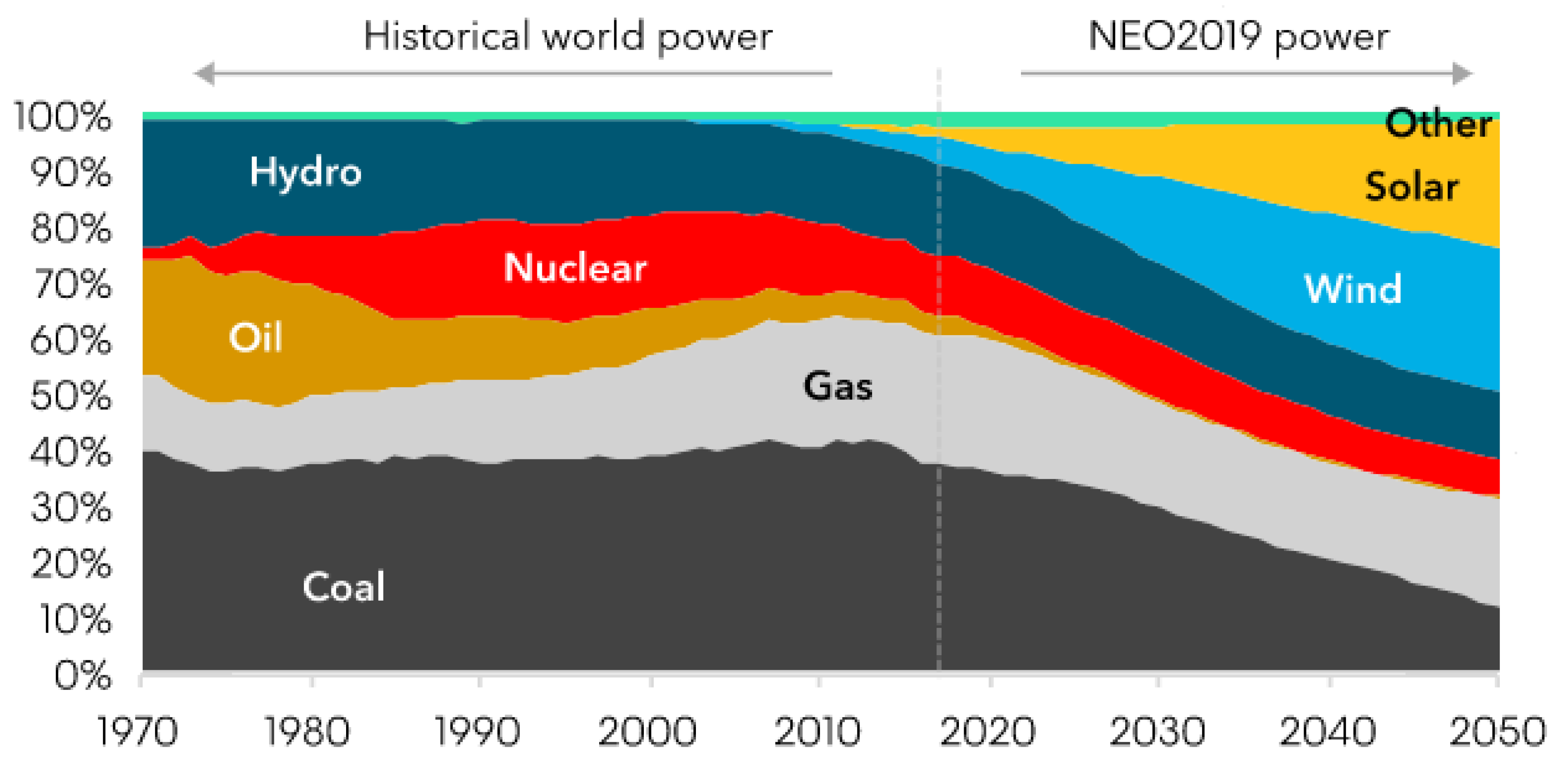
Figure 1.
Forecast of the percentage share of various energy carriers in the global energy mix by 2050. Source: own study based on [
1].
Figure 1.
Forecast of the percentage share of various energy carriers in the global energy mix by 2050. Source: own study based on [
1].
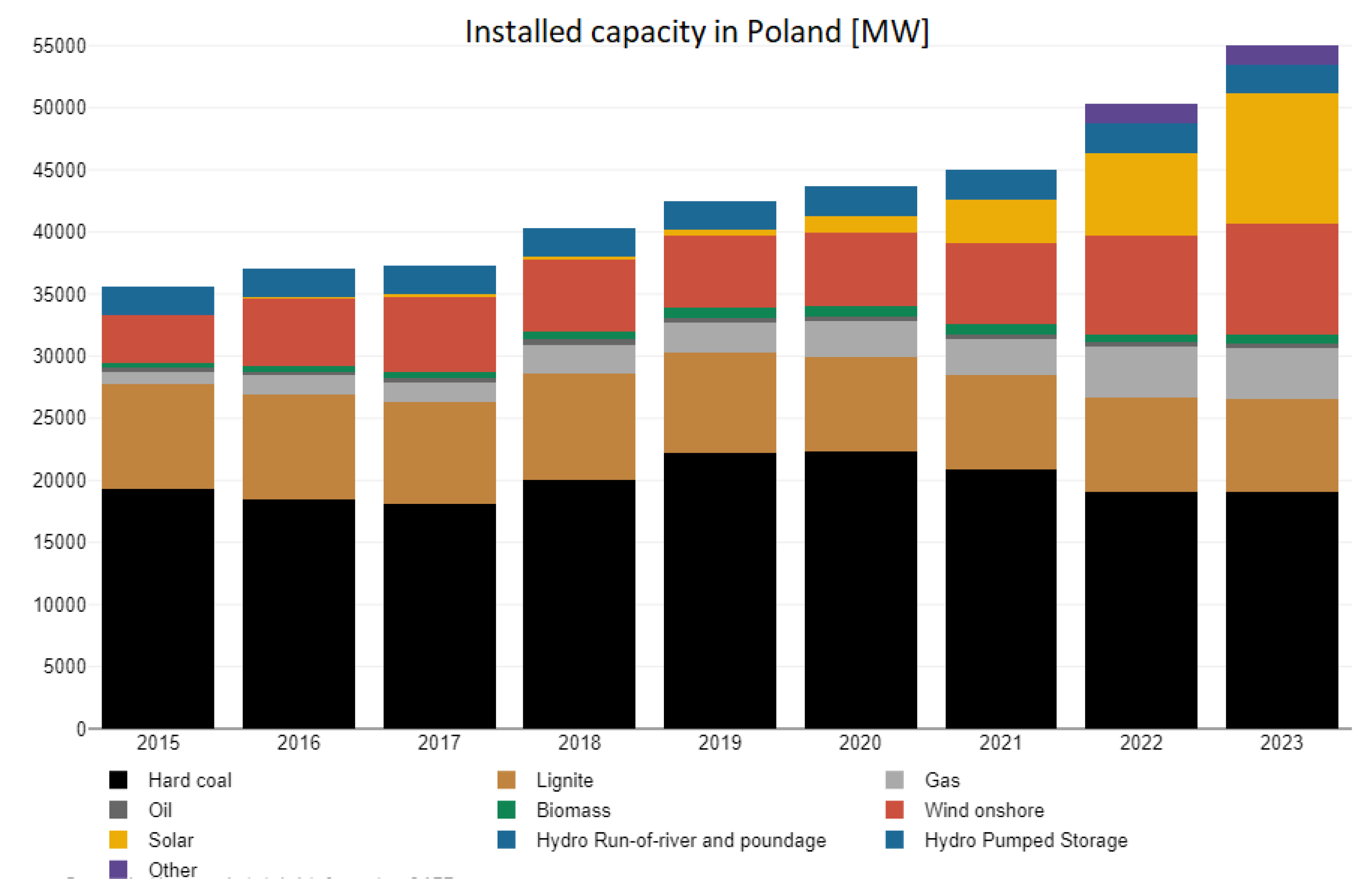
Figure 2.
Installed capacity in Poland broken down by individual energy sources. Source: own study based on [
2].
Figure 2.
Installed capacity in Poland broken down by individual energy sources. Source: own study based on [
2].
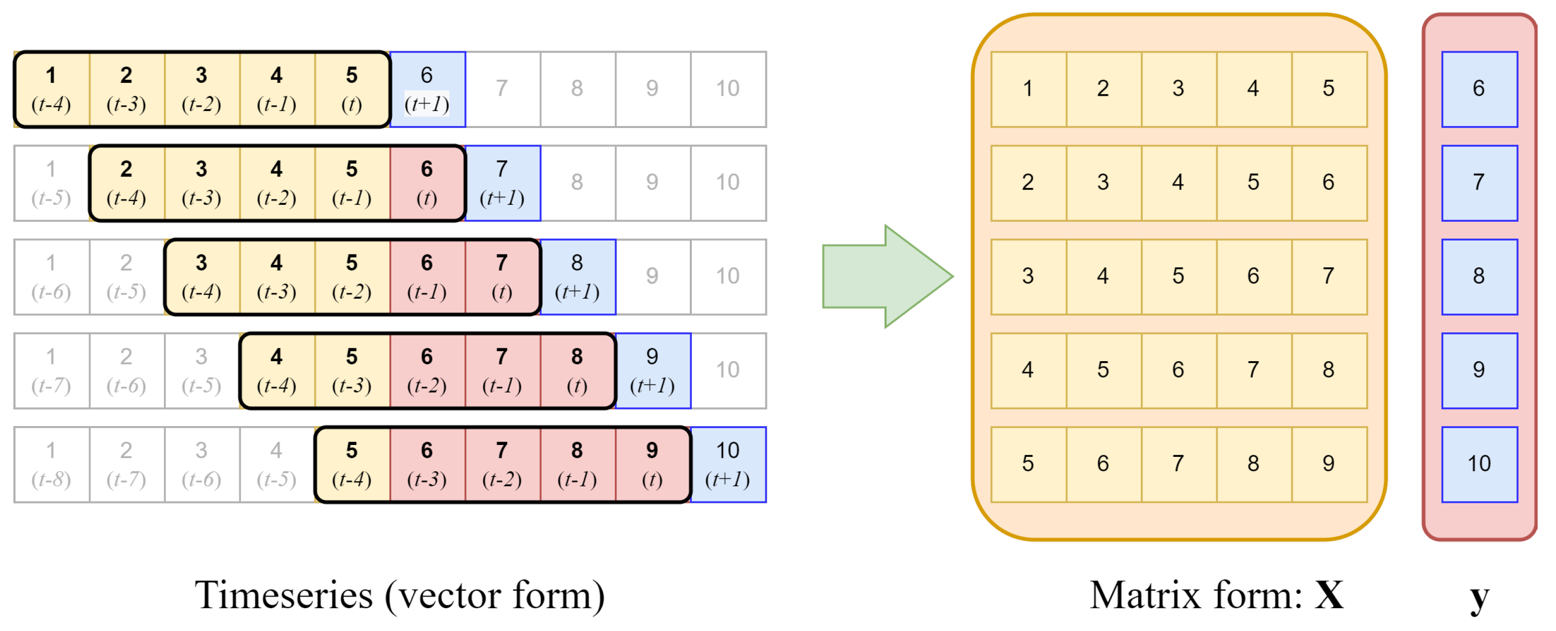
Figure 3.
Scheme of transforming a time series vector into a matrix form suitable for regression models.
Figure 3.
Scheme of transforming a time series vector into a matrix form suitable for regression models.
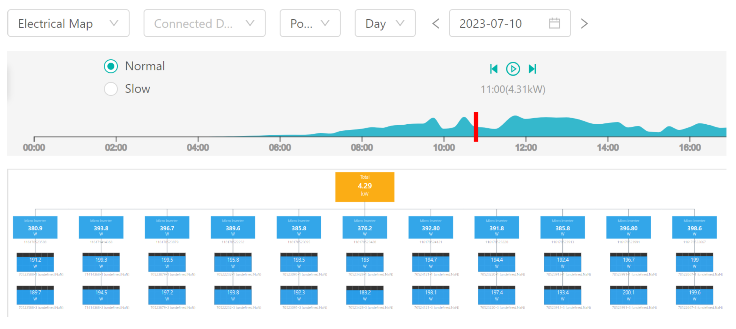
Figure 4.
Diagram of the connections of a photovoltaic power plant.
Figure 4.
Diagram of the connections of a photovoltaic power plant.
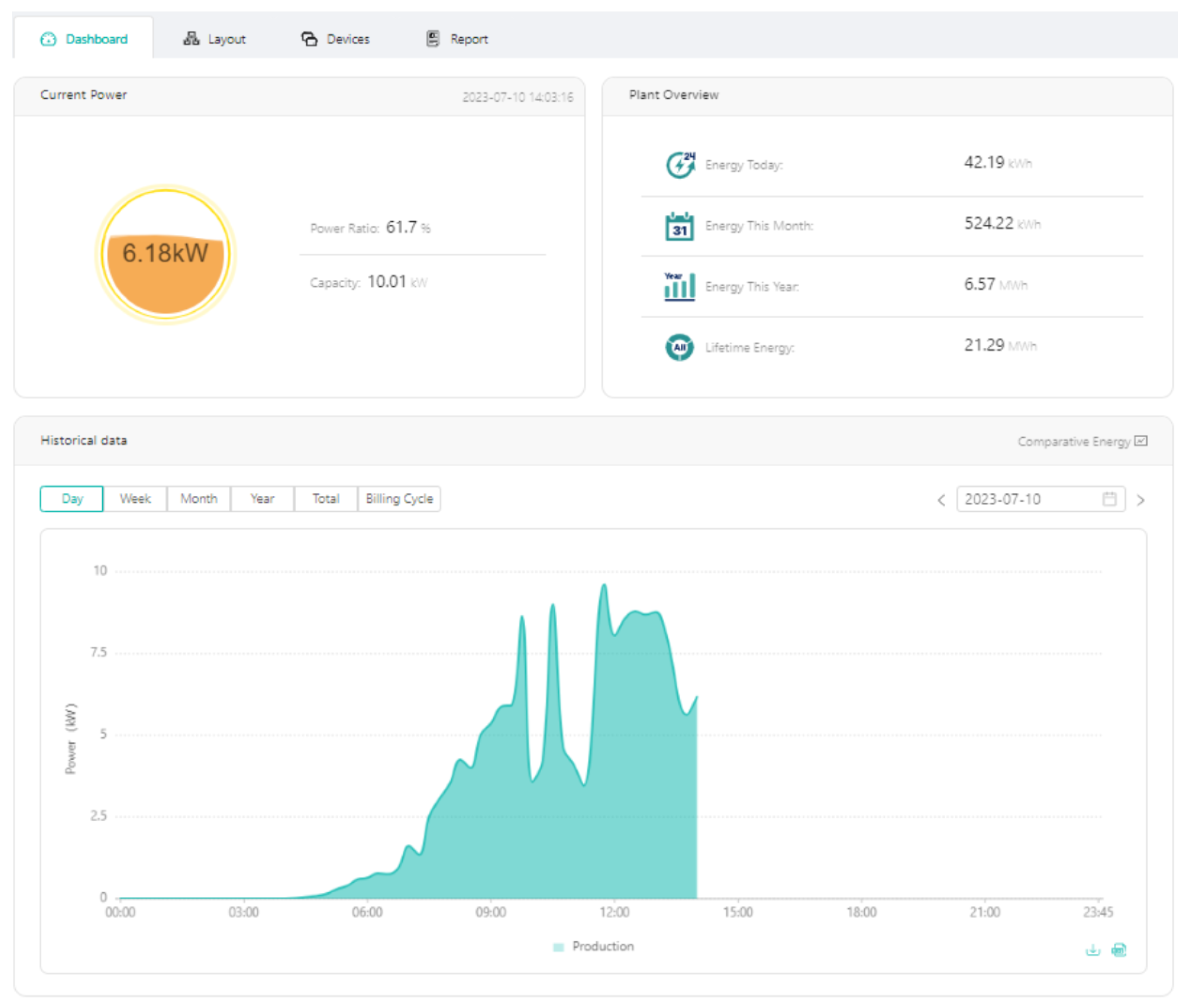
Figure 5.
The application for monitoring the photovoltaic power plant.
Figure 5.
The application for monitoring the photovoltaic power plant.
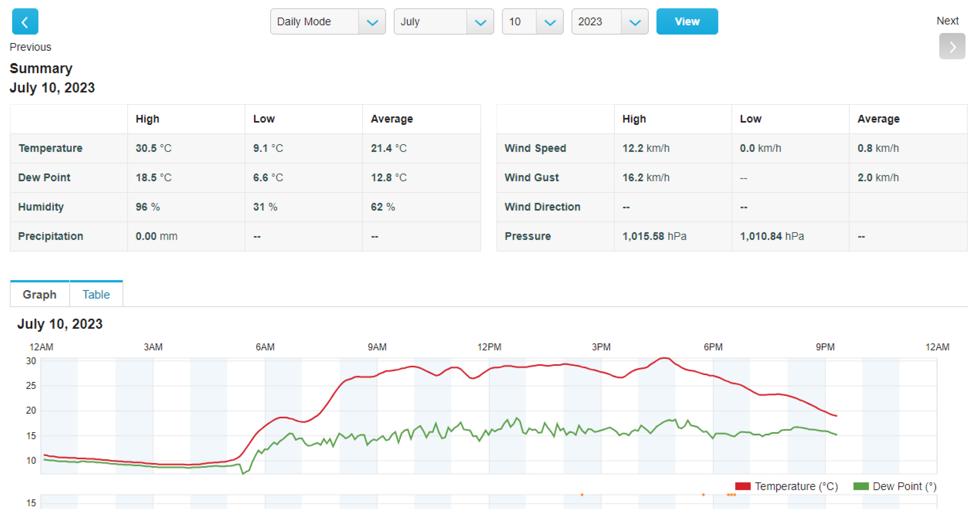
Figure 6.
Weather station start screen.
Figure 6.
Weather station start screen.
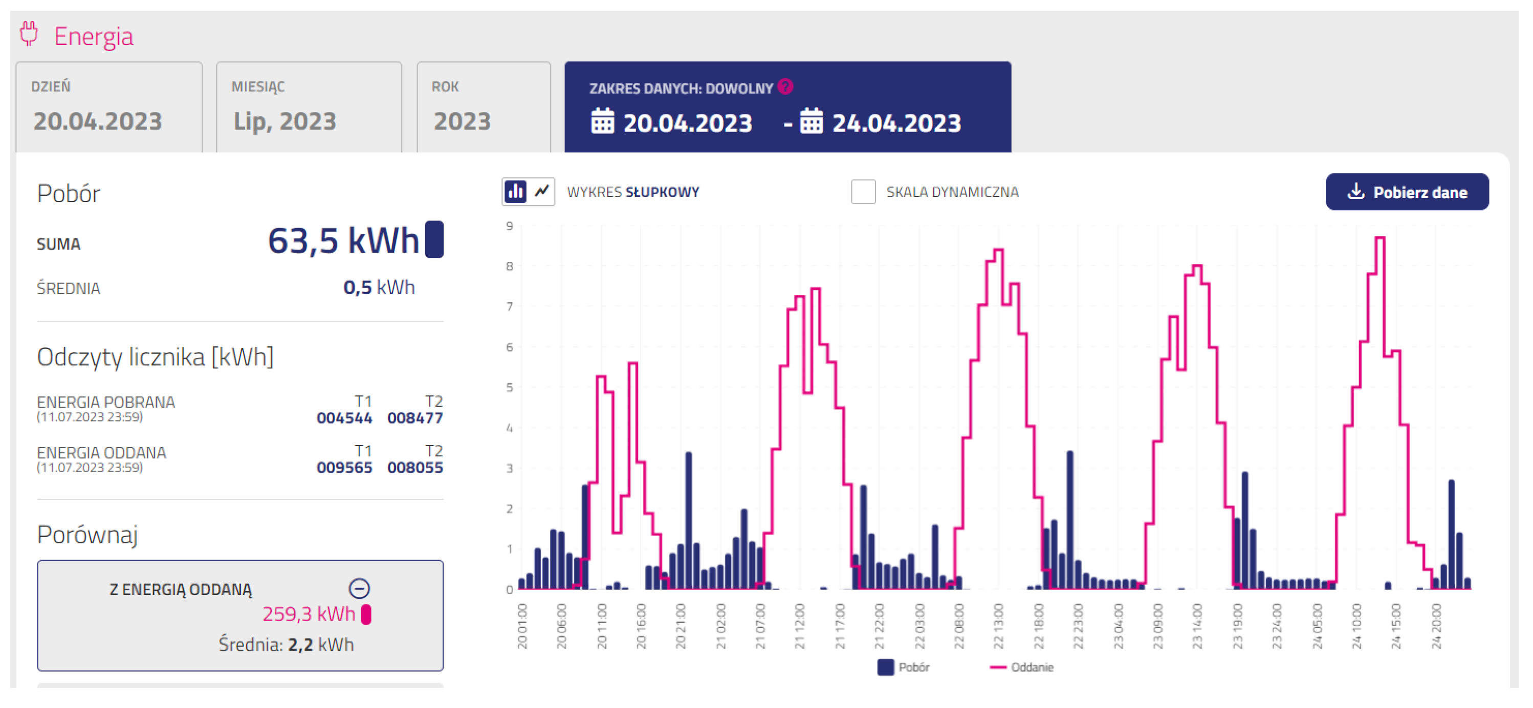
Figure 7.
Values of energy produced and consumed in hourly time intervals.
Figure 7.
Values of energy produced and consumed in hourly time intervals.
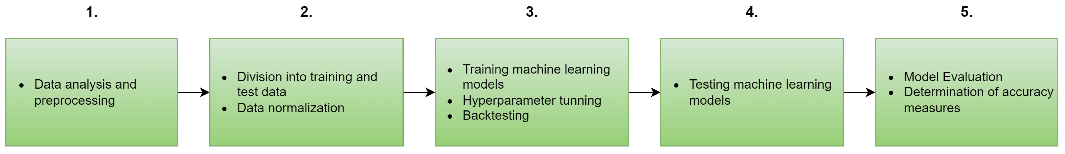
Figure 8.
Research methodology workflow diagram.
Figure 8.
Research methodology workflow diagram.
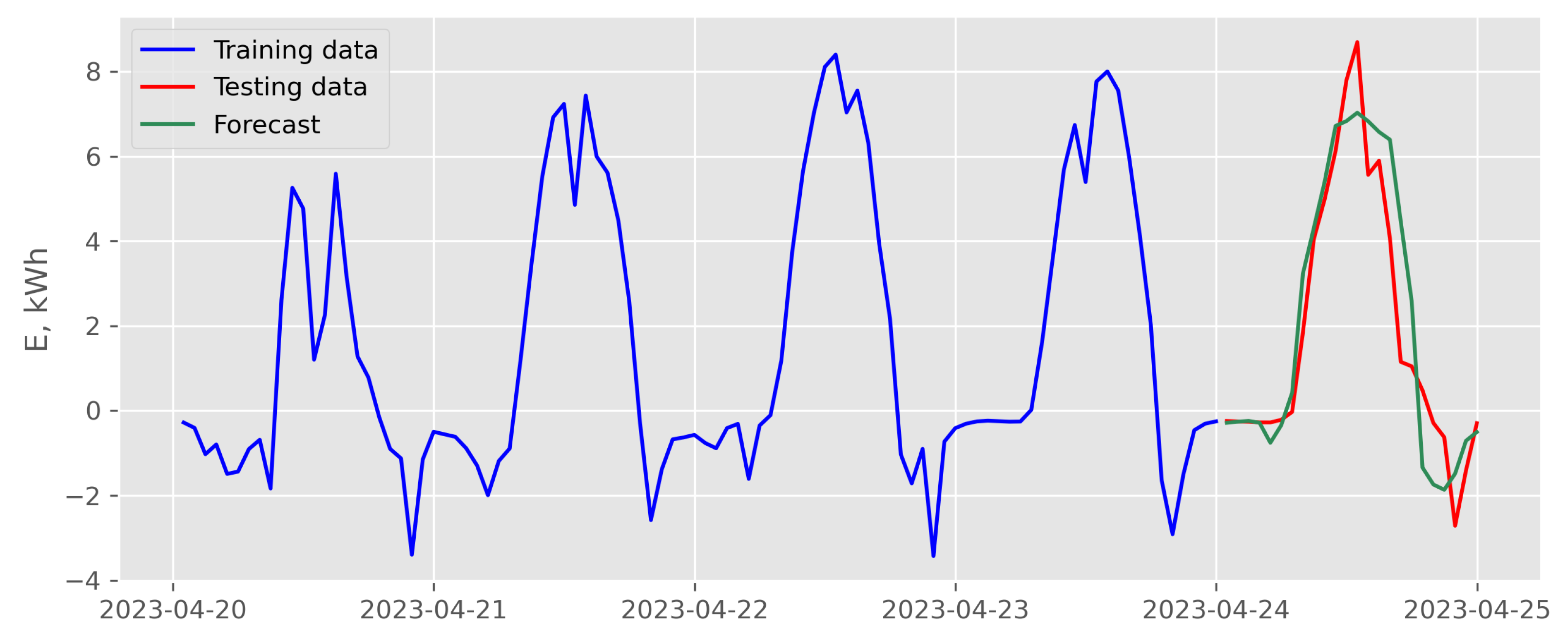
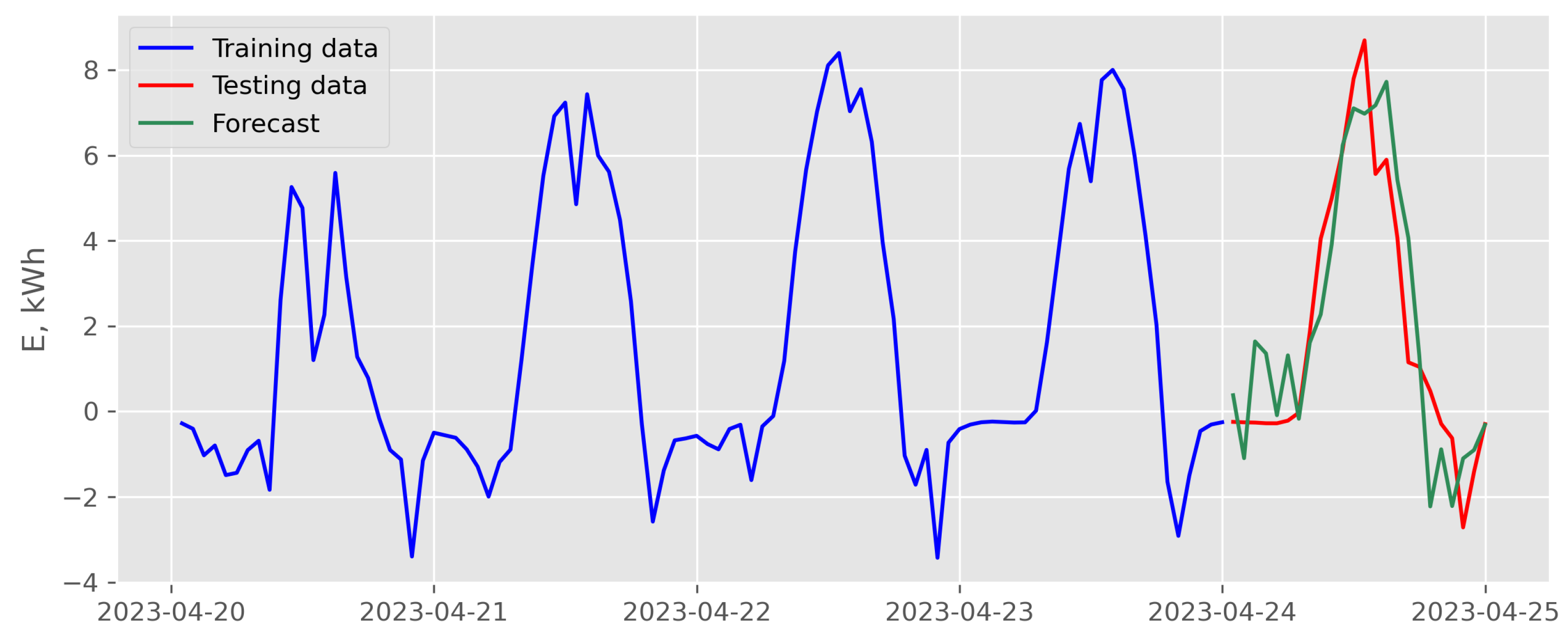
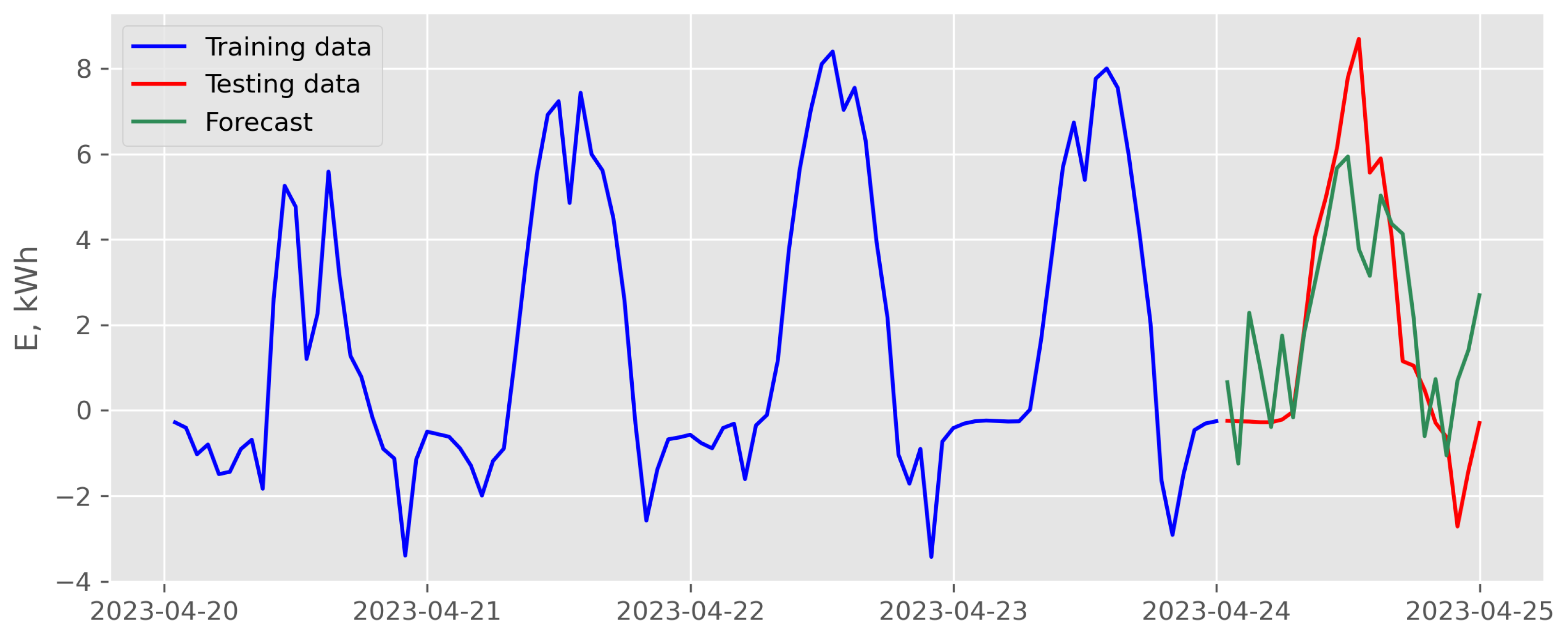
Figure 9.
Results of recursive multi-step forecasting with LASSO model and endogenous scenario for data recorded in April 2023 (case of the best backtesting MSE).
Figure 9.
Results of recursive multi-step forecasting with LASSO model and endogenous scenario for data recorded in April 2023 (case of the best backtesting MSE).
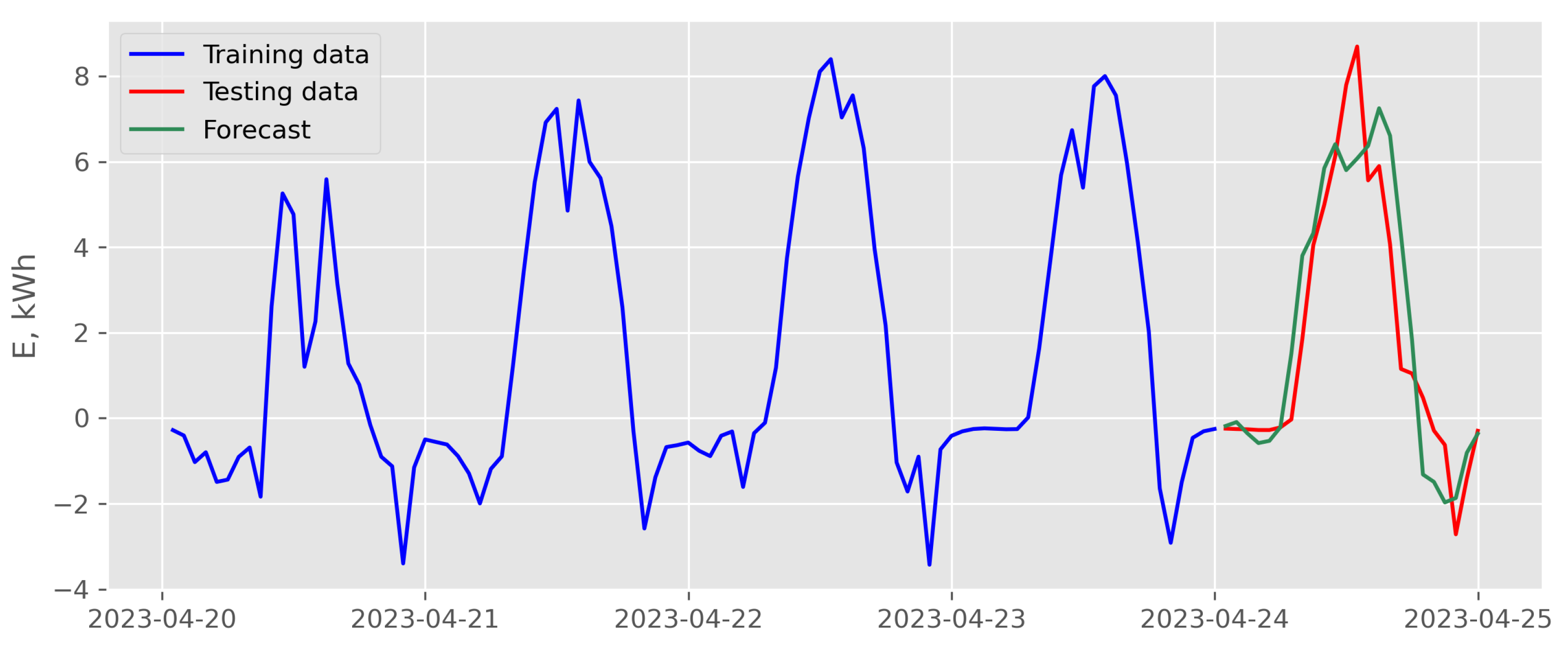
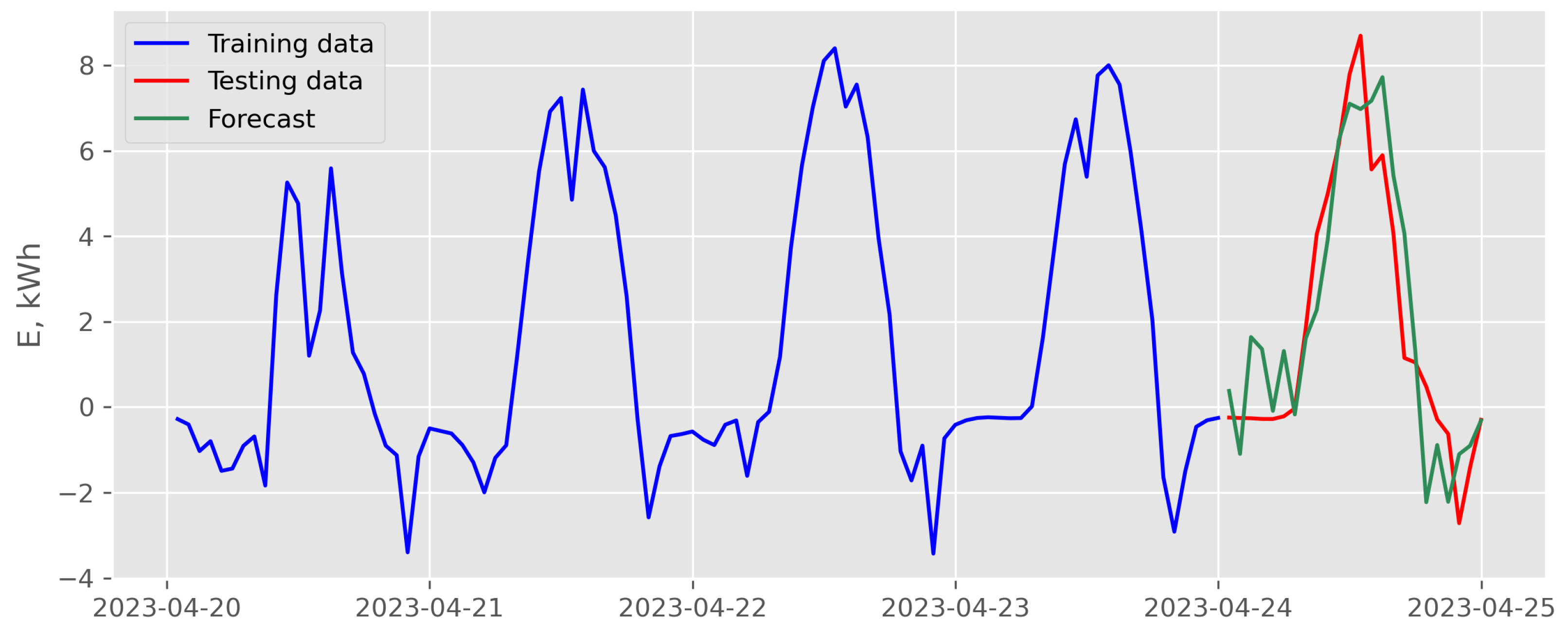
Figure 10.
Results of recursive multi-step forecasting with LASSO model and exogenous variables scenario for data recorded in April 2023 (case of the best backtesting MSE).
Figure 10.
Results of recursive multi-step forecasting with LASSO model and exogenous variables scenario for data recorded in April 2023 (case of the best backtesting MSE).
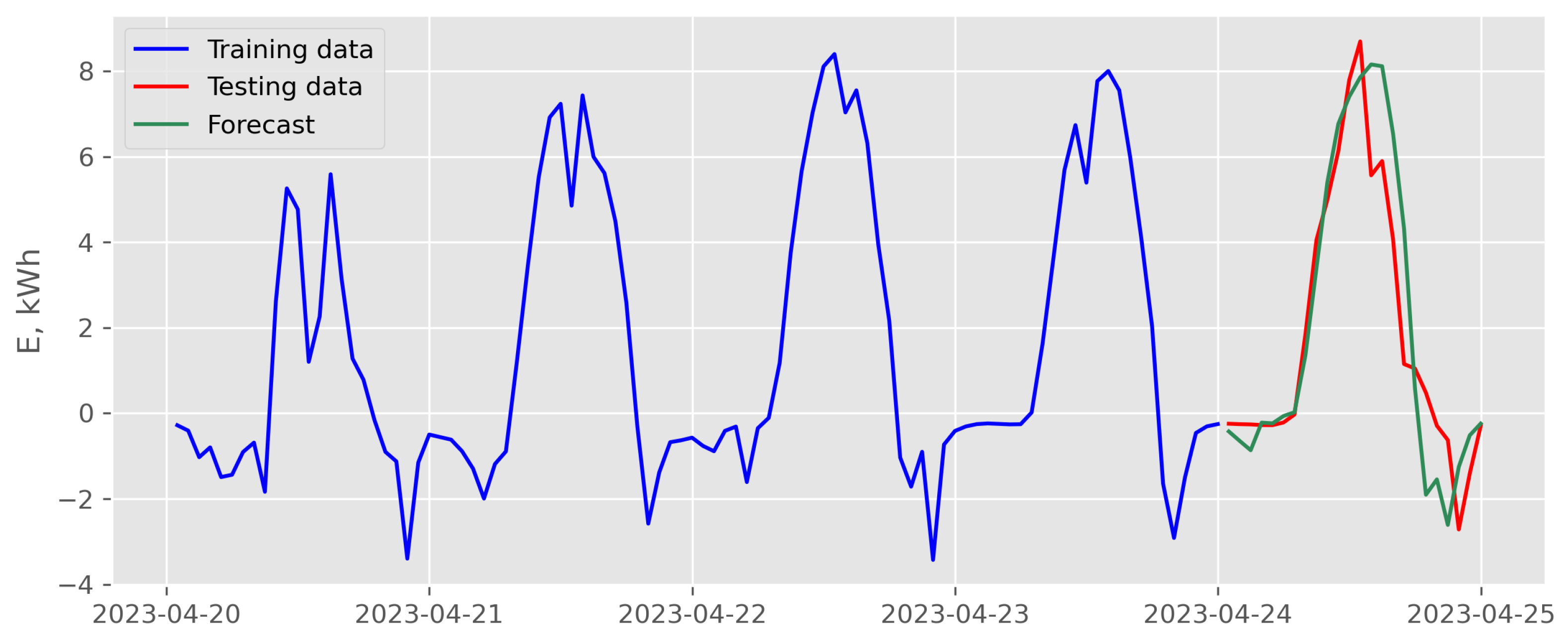
Figure 11.
Results of direct multi-step forecasting with LASSO model and endogenous scenario for data recorded in April 2023 (case of the best backtesting MSE).
Figure 11.
Results of direct multi-step forecasting with LASSO model and endogenous scenario for data recorded in April 2023 (case of the best backtesting MSE).
Figure 12.
Results of direct multi-step forecasting with LASSO model and exogenous variables scenario for data recorded in April 2023 (case of the best backtesting MSE).
Figure 12.
Results of direct multi-step forecasting with LASSO model and exogenous variables scenario for data recorded in April 2023 (case of the best backtesting MSE).
Figure 13.
Results of recursive multi-step forecasting with random forest model and endogenous scenario for data recorded in April 2023 (case of the best backtesting MSE).
Figure 13.
Results of recursive multi-step forecasting with random forest model and endogenous scenario for data recorded in April 2023 (case of the best backtesting MSE).
Figure 14.
Results of recursive multi-step forecasting with random forest model and exogenous variables scenario for data recorded in April 2023 (case of the best backtesting MSE).
Figure 14.
Results of recursive multi-step forecasting with random forest model and exogenous variables scenario for data recorded in April 2023 (case of the best backtesting MSE).
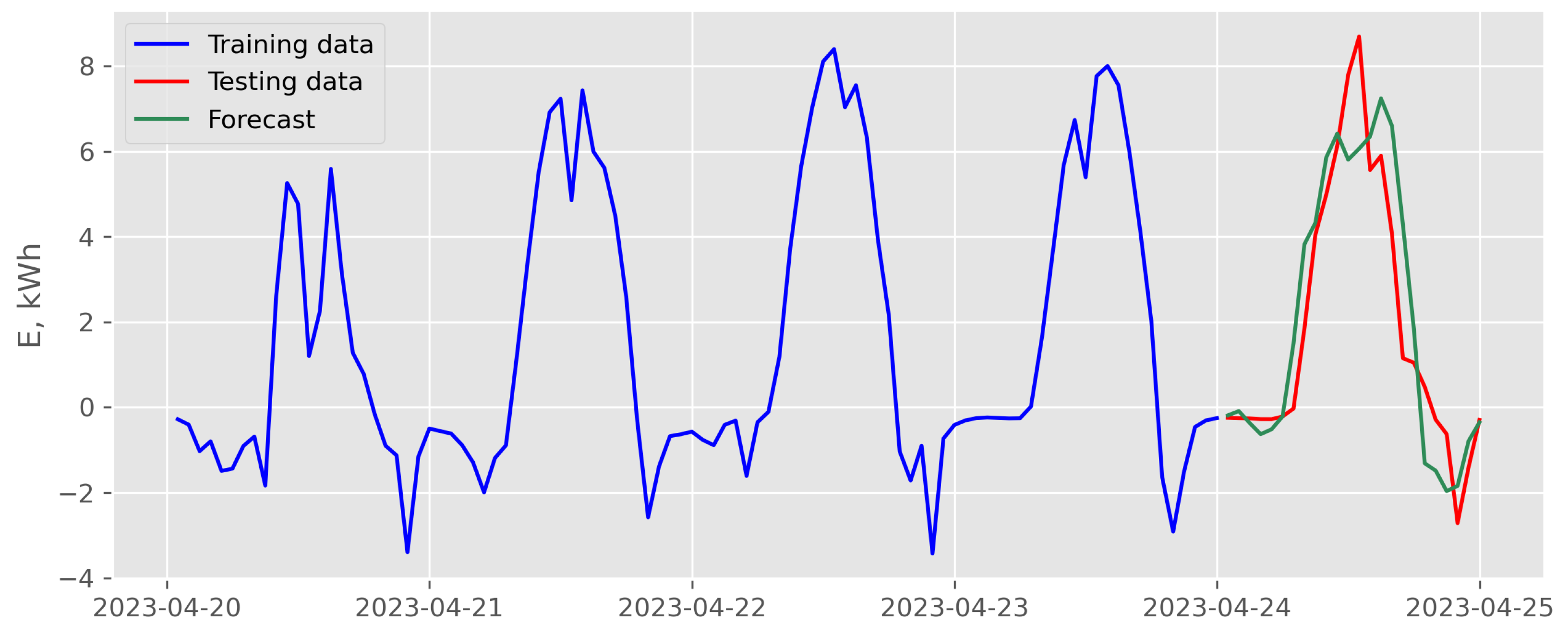
Figure 15.
Results of direct multi-step forecasting with random forest model and endogenous scenario for data recorded in April 2023 (case of the best backtesting MSE).
Figure 15.
Results of direct multi-step forecasting with random forest model and endogenous scenario for data recorded in April 2023 (case of the best backtesting MSE).
Figure 16.
Results of direct multi-step forecasting with random forest model and exogenous variables scenario for data recorded in April 2023 (case of the best backtesting MSE).
Figure 16.
Results of direct multi-step forecasting with random forest model and exogenous variables scenario for data recorded in April 2023 (case of the best backtesting MSE).
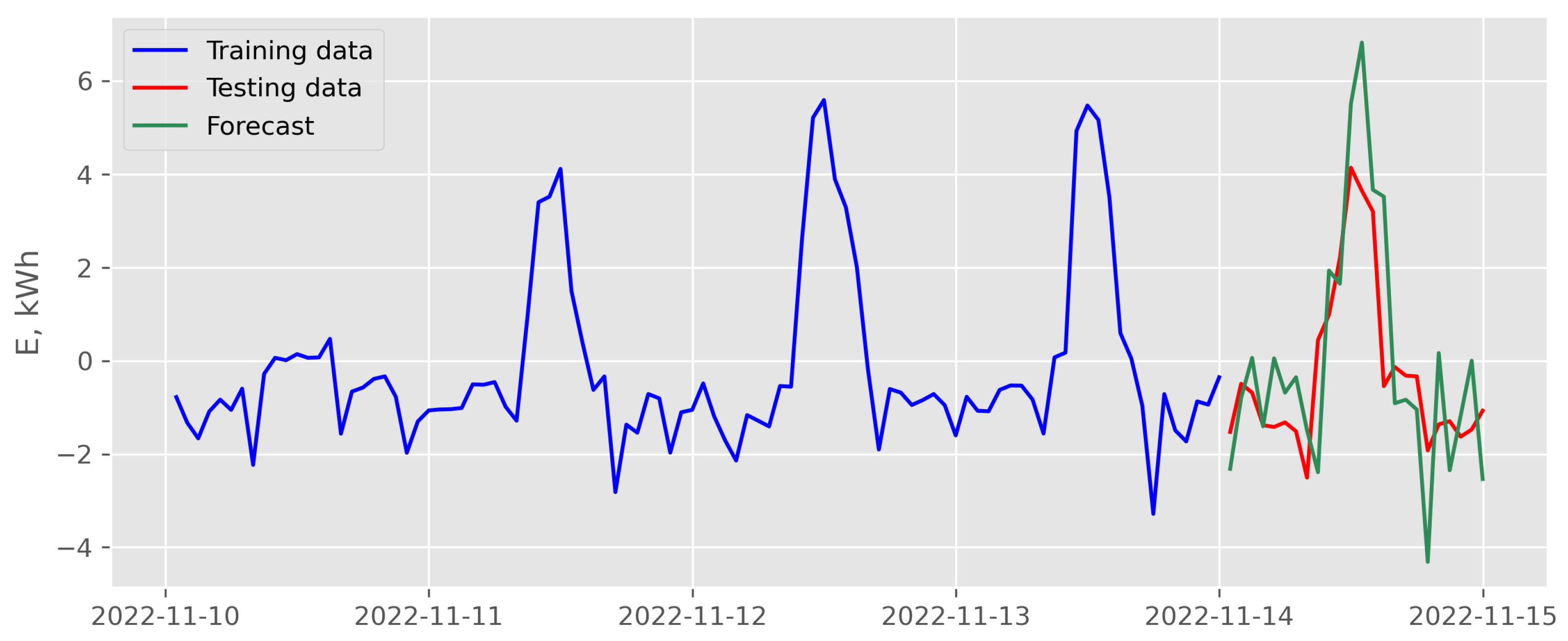
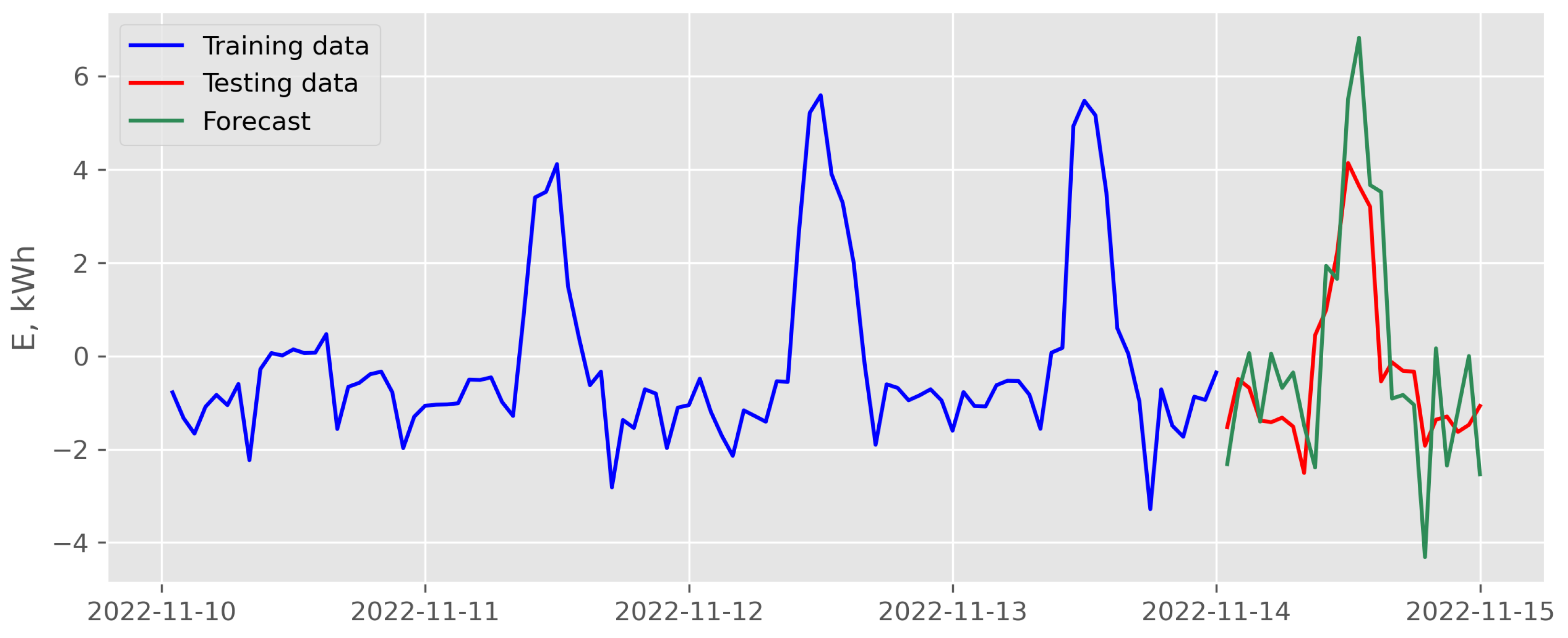
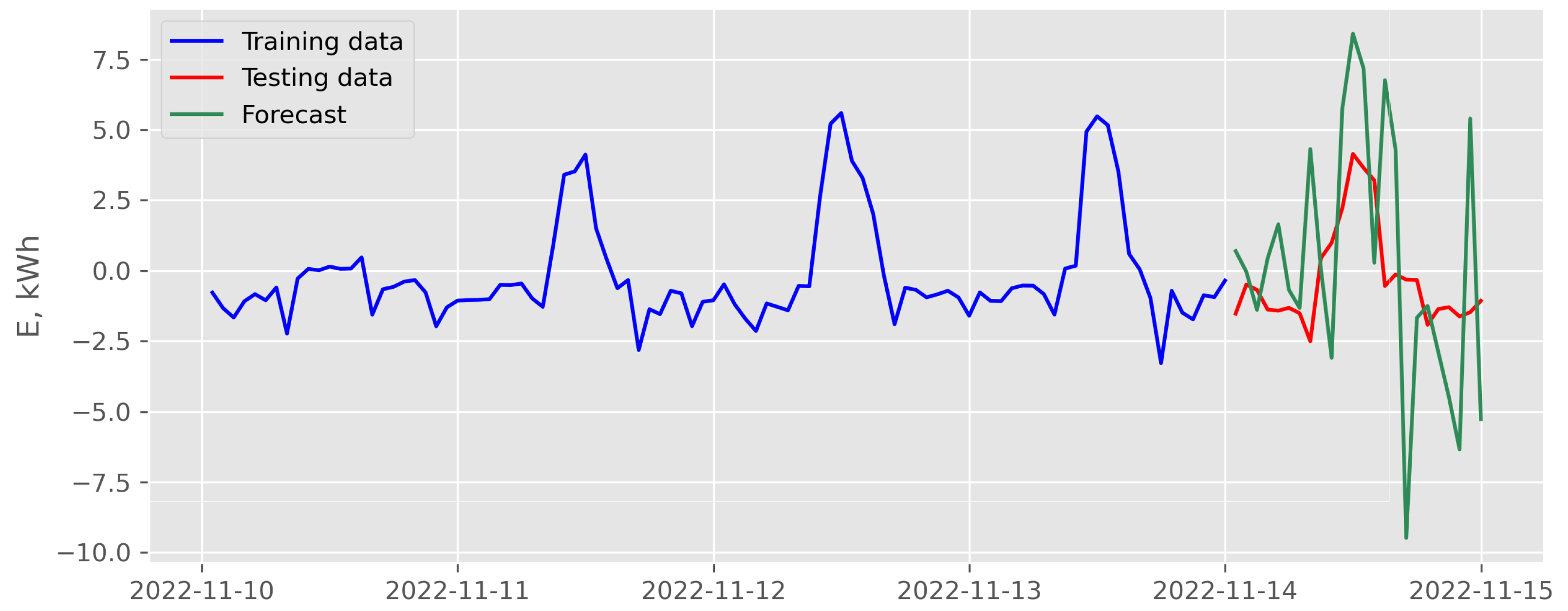
Figure 17.
Results of recursive multi-step forecasting with LASSO and endogenous scenario for data recorded in November 2022 (case of the best backtesting MSE).
Figure 17.
Results of recursive multi-step forecasting with LASSO and endogenous scenario for data recorded in November 2022 (case of the best backtesting MSE).
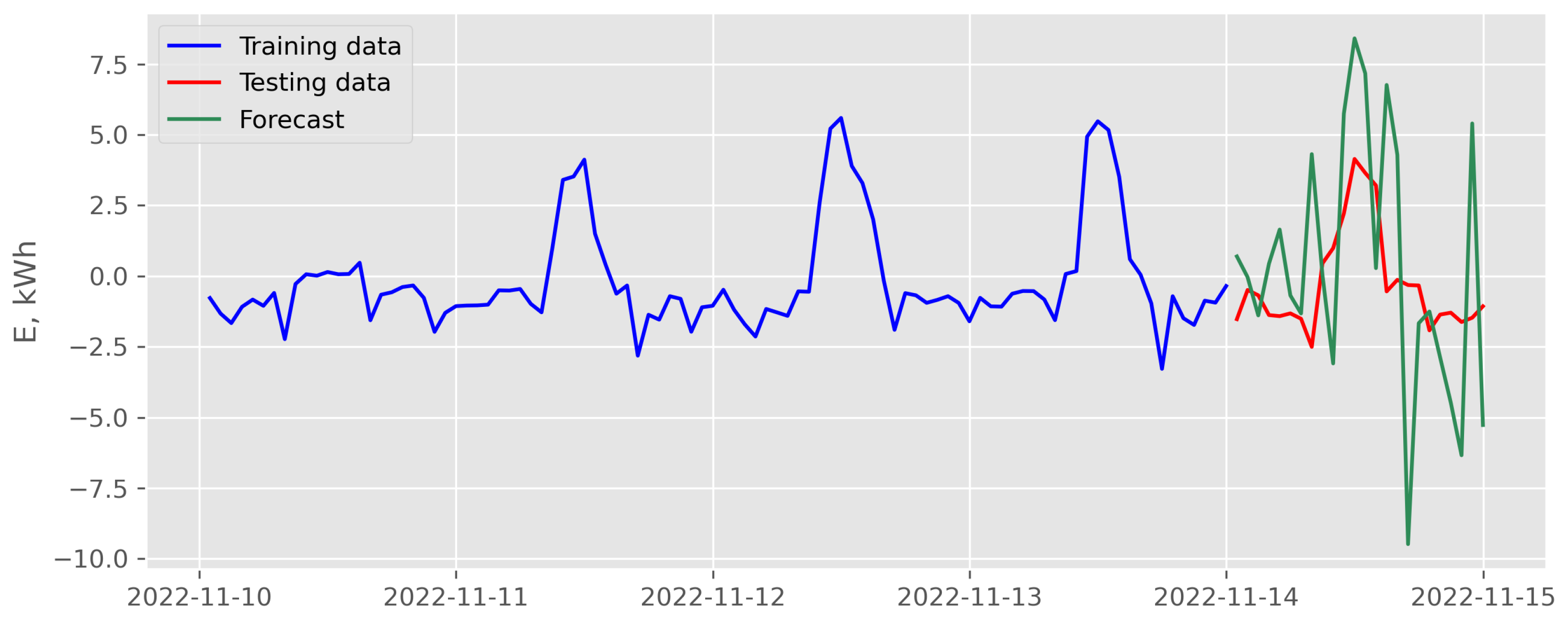
Figure 18.
Results of recursive multi-step forecasting with LASSO and exogenous variables scenario for data recorded in November 2022 (case of the best backtesting MSE).
Figure 18.
Results of recursive multi-step forecasting with LASSO and exogenous variables scenario for data recorded in November 2022 (case of the best backtesting MSE).
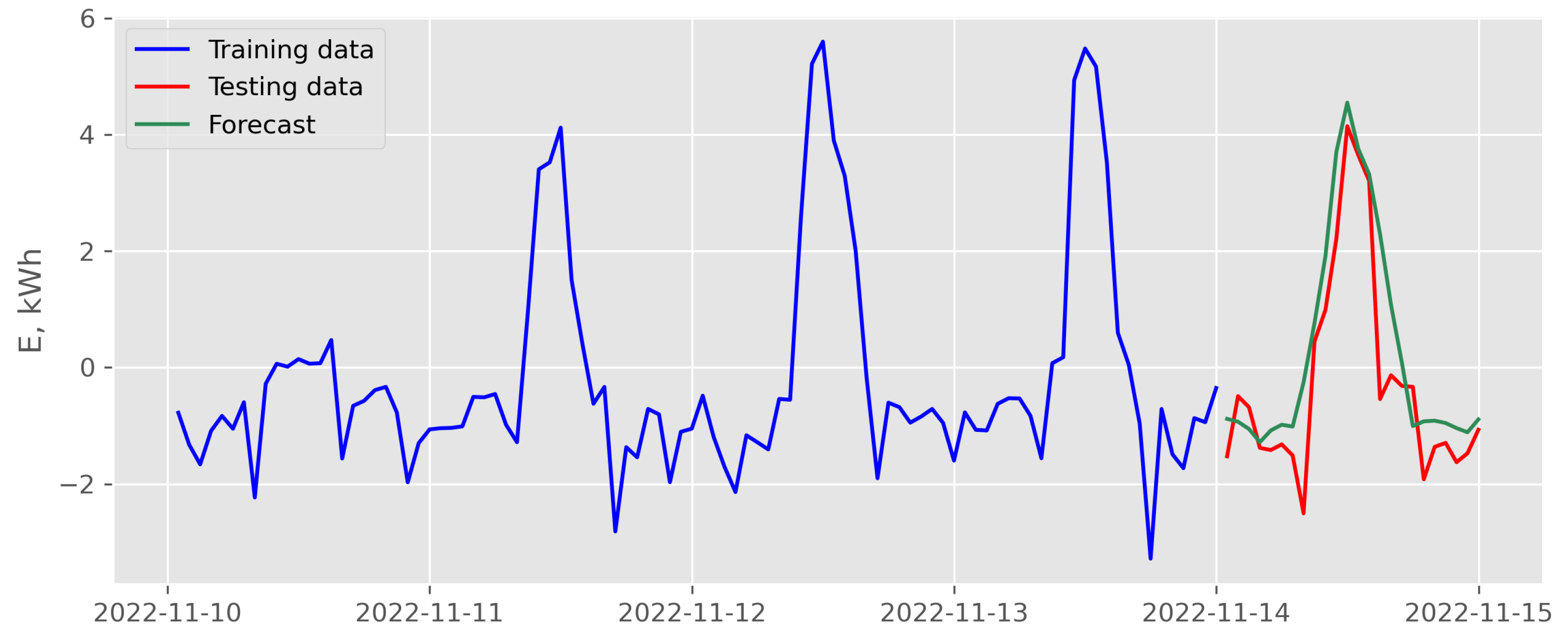
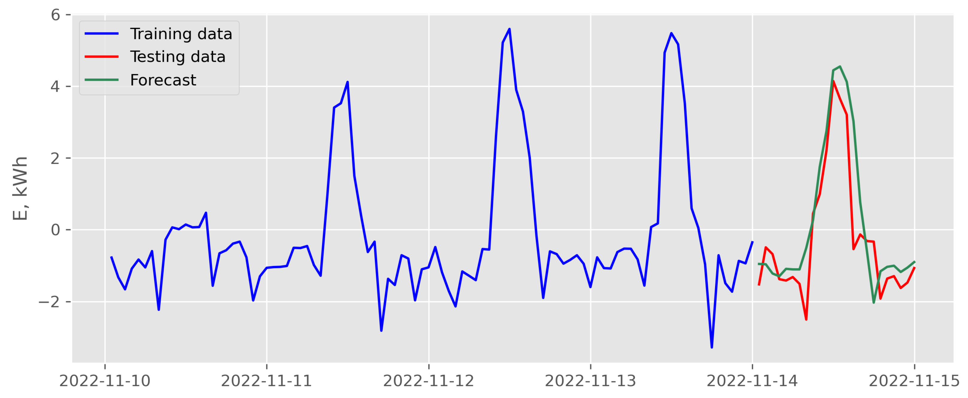
Figure 19.
Results of direct multi-step forecasting with LASSO and endogenous scenario for data recorded in November 2022 (case of the best backtesting MSE).
Figure 19.
Results of direct multi-step forecasting with LASSO and endogenous scenario for data recorded in November 2022 (case of the best backtesting MSE).
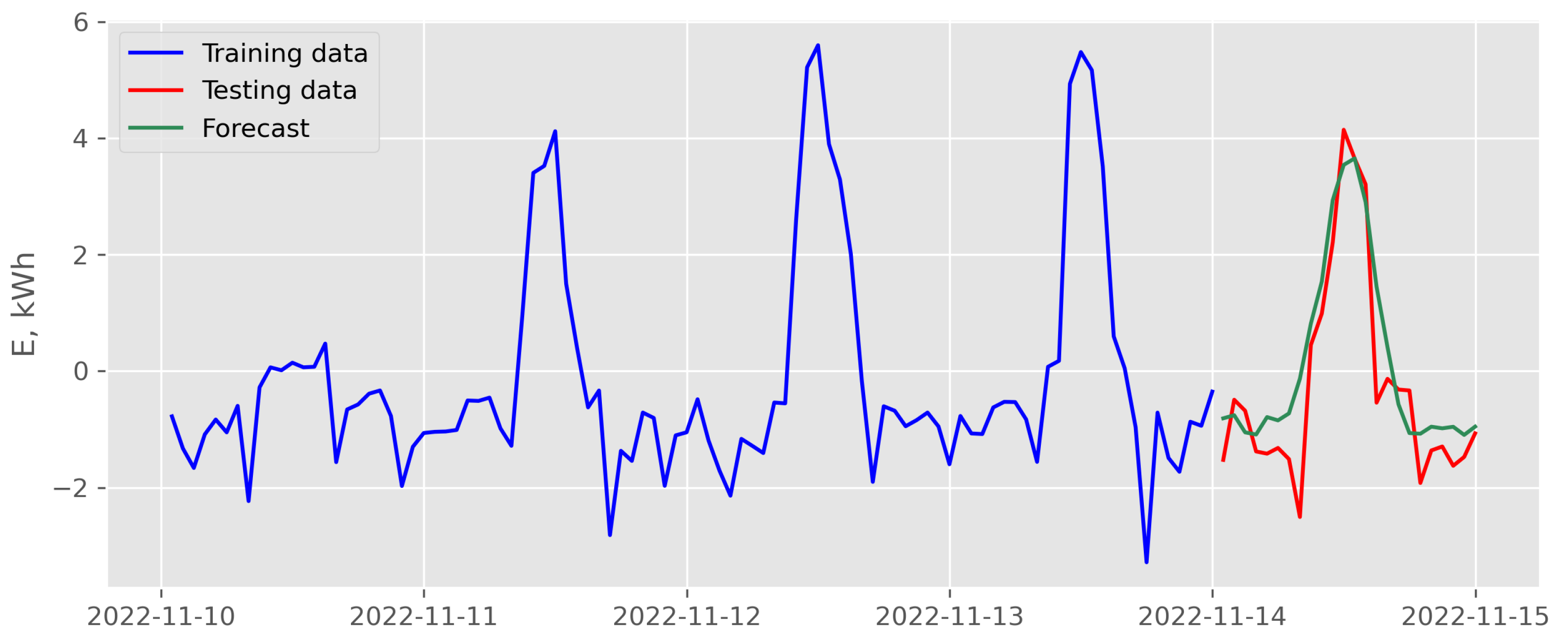
Figure 20.
Results of direct multi-step forecasting with LASSO and exogenous variables scenario for data recorded in November 2022 (case of the best backtesting MSE).
Figure 20.
Results of direct multi-step forecasting with LASSO and exogenous variables scenario for data recorded in November 2022 (case of the best backtesting MSE).
Figure 21.
Results of recursive multi-step forecasting with random forest and endogenous scenario for data recorded in November 2022 (case of the best backtesting MSE).
Figure 21.
Results of recursive multi-step forecasting with random forest and endogenous scenario for data recorded in November 2022 (case of the best backtesting MSE).
Figure 22.
Results of recursive multi-step forecasting with random forest and exogenous variables scenario for data recorded in November 2022 (case of the best backtesting MSE).
Figure 22.
Results of recursive multi-step forecasting with random forest and exogenous variables scenario for data recorded in November 2022 (case of the best backtesting MSE).
Figure 23.
Results of direct multi-step forecasting with random forest and endogenous scenario for data recorded in November 2022 (case of the best backtesting MSE).
Figure 23.
Results of direct multi-step forecasting with random forest and endogenous scenario for data recorded in November 2022 (case of the best backtesting MSE).
Figure 24.
Results of direct multi-step forecasting with random forest and exogenous variables scenario for data recorded in November 2022 (case of the best backtesting MSE).
Figure 24.
Results of direct multi-step forecasting with random forest and exogenous variables scenario for data recorded in November 2022 (case of the best backtesting MSE).
Table 1.
Evaluation results of LASSO model for data recorded in April 2023 (case of recursive multi-step forecasting with endogenous scenario).
Table 1.
Evaluation results of LASSO model for data recorded in April 2023 (case of recursive multi-step forecasting with endogenous scenario).
| | | | l |
|---|
| 1.05 | 1.96 | 1.14 | 36 |
| 2.61 | 1.45 | 0.85 | 24 |
| 16.50 | 9.57 | 2.71 | 24 |
Table 2.
Evaluation results of LASSO model for data recorded in April 2023 (case of recursive multi-step forecasting with exogenous variables scenario).
Table 2.
Evaluation results of LASSO model for data recorded in April 2023 (case of recursive multi-step forecasting with exogenous variables scenario).
| | | | Exogenous | l |
|---|
| 1.23 | 1.96 | 1.14 | | 36 |
| 2.01 | 1.96 | 1.14 | | 36 |
| 12.9 | 9.58 | 2.74 | | 36 |
Table 3.
Evaluation results of LASSO model for data recorded in April 2023 (case of direct multi-step forecasting with endogenous scenario).
Table 3.
Evaluation results of LASSO model for data recorded in April 2023 (case of direct multi-step forecasting with endogenous scenario).
| | | | l |
|---|
| 1.18 | 3.80 | 1.52 | 36 |
| 3.58 | 1.87 | 0.99 | 24 |
| 18.0 | 8.27 | 2.52 | 36 |
Table 4.
Evaluation results of LASSO model for data recorded in April 2023 (case of direct multi-step forecasting with exogenous variables scenario).
Table 4.
Evaluation results of LASSO model for data recorded in April 2023 (case of direct multi-step forecasting with exogenous variables scenario).
| | | | Exogenous | l |
|---|
| 1.49 | 1.87 | 0.99 | , | 24 |
| 2.73 | 3.80 | 1.52 | | 36 |
| 15.6 | 8.27 | 2.52 | | 36 |
Table 5.
Evaluation results of random forest model for data recorded in April 2023 (case of recursive multi-step forecasting with endogenous scenario).
Table 5.
Evaluation results of random forest model for data recorded in April 2023 (case of recursive multi-step forecasting with endogenous scenario).
| | | | | | l |
|---|
| 297 | 49.0 | 0.90 | 1.52 | 0.92 | all | 36 |
| 29 | 46.0 | 1.68 | 1.05 | 0.82 | sqrt | 24 |
| 315 | 23.0 | 2.03 | 1.02 | 0.77 | log2 | 24 |
Table 6.
Evaluation results of random forest model for data recorded in April 2023 (case of recursive multi-step forecasting with exogenous variables scenario).
Table 6.
Evaluation results of random forest model for data recorded in April 2023 (case of recursive multi-step forecasting with exogenous variables scenario).
| | | | | | Exogenous | l |
|---|
| 100 | 17 | 0.88 | 1.52 | 0.92 | all | | 36 |
| 49 | 42 | 1.53 | 1.11 | 0.76 | log2 | ,
| 36 |
| 55 | 15 | 3.26 | 1.14 | 0.79 | log2 | | 36 |
Table 7.
Evaluation results of random forest model for data recorded in April 2023 (case of direct multi-step forecasting with endogenous scenario).
Table 7.
Evaluation results of random forest model for data recorded in April 2023 (case of direct multi-step forecasting with endogenous scenario).
| | | | | | l |
|---|
| 377 | 13 | 0.98 | 1.88 | 1.04 | all | 24 |
| 361 | 5 | 2.06 | 1.61 | 0.85 | log2 | 24 |
| 361 | 5 | 3.49 | 1.51 | 0.80 | log2 | 36 |
Table 8.
Evaluation results of random forest model for data recorded in April 2023 (case of direct multi-step forecasting with exogenous variables scenario).
Table 8.
Evaluation results of random forest model for data recorded in April 2023 (case of direct multi-step forecasting with exogenous variables scenario).
| | | | | | Exogenous | l |
|---|
| 392 | 29 | 0.96 | 1.87 | 1.03 | all | | 24 |
| 472 | 49 | 1.89 | 1.65 | 0.86 | sqrt | | 24 |
| 496 | 47 | 3.21 | 1.49 | 0.79 | log2 | ,
| 36 |
Table 9.
Evaluation results of LASSO model for data recorded in November 2022 (case of recursive multi-step forecasting with endogenous scenario).
Table 9.
Evaluation results of LASSO model for data recorded in November 2022 (case of recursive multi-step forecasting with endogenous scenario).
| | | | l |
|---|
| 1.60 | 2.47 | 1.25 | 36 |
| 5.87 | 2.47 | 1.25 | 36 |
| 25.5 | 2.47 | 1.25 | 36 |
Table 10.
Evaluation results of LASSO model for data recorded in November 2022 (case of recursive multi-step forecasting with exogenous variables scenario).
Table 10.
Evaluation results of LASSO model for data recorded in November 2022 (case of recursive multi-step forecasting with exogenous variables scenario).
| | | | Exogenous | l |
|---|
| 1.58 | 2.47 | 1.24 | | 36 |
| 3.10 | 1.39 | 0.92 | | 24 |
| 40.8 | 2.47 | 1.24 | , | 36 |
Table 11.
Evaluation results of LASSO model for data recorded in November 2022 (case of direct multi-step forecasting with endogenous scenario).
Table 11.
Evaluation results of LASSO model for data recorded in November 2022 (case of direct multi-step forecasting with endogenous scenario).
| | | | l |
|---|
| 0.61 | 16.4 | 3.25 | 36 |
| 2.95 | 16.4 | 3.25 | 36 |
| 8.92 | 3.29 | 1.57 | 36 |
Table 12.
Evaluation results of LASSO model for data recorded in November 2022 (case of direct multi-step forecasting with exogenous variables scenario).
Table 12.
Evaluation results of LASSO model for data recorded in November 2022 (case of direct multi-step forecasting with exogenous variables scenario).
| | | | Exogenous | l |
|---|
| 0.62 | 16.3 | 3.25 | | 36 |
| 3.36 | 16.3 | 3.25 | , | 36 |
| 13.4 | 2.67 | 1.14 | , | 24 |
Table 13.
Evaluation results of random forest model for data recorded in November 2022 (case of recursive multi-step forecasting with endogenous scenario).
Table 13.
Evaluation results of random forest model for data recorded in November 2022 (case of recursive multi-step forecasting with endogenous scenario).
| | | | | | l |
|---|
| 75 | 14 | 1.79 | 0.90 | 0.68 | all | 24 |
| 343 | 10 | 3.00 | 1.12 | 0.78 | all | 36 |
| 21 | 7 | 4.69 | 0.84 | 0.69 | sqrt | 36 |
Table 14.
Evaluation results of random forest model for data recorded in November 2022 (case of recursive multi-step forecasting with exogenous variables scenario).
Table 14.
Evaluation results of random forest model for data recorded in November 2022 (case of recursive multi-step forecasting with exogenous variables scenario).
| | | | | | Exogenous | l |
|---|
| 197 | 15 | 1.74 | 0.64 | 0.61 | sqrt | | 24 |
| 117 | 17 | 2.65 | 1.08 | 0.75 | all | | 36 |
| 100 | 17 | 3.78 | 0.99 | 0.72 | all | | 24 |
Table 15.
Evaluation results of random forest model for data recorded in November 2022 (case of direct multi-step forecasting with endogenous scenario).
Table 15.
Evaluation results of random forest model for data recorded in November 2022 (case of direct multi-step forecasting with endogenous scenario).
| | | | | | l |
|---|
| 343 | 10 | 1.52 | 1.02 | 0.68 | all | 24 |
| 75 | 14 | 3.06 | 1.09 | 0.72 | all | 36 |
| 457 | 9 | 5.48 | 0.90 | 0.69 | log2 | 36 |
Table 16.
Evaluation results of random forest model for data recorded in November 2022 (case of direct multi-step forecasting with exogenous variables scenario).
Table 16.
Evaluation results of random forest model for data recorded in November 2022 (case of direct multi-step forecasting with exogenous variables scenario).
| | | | | | Exogenous | l |
|---|
| 201 | 20 | 1.55 | 1.0 | 0.71 | all | | 24 |
| 117 | 17 | 2.89 | 1.04 | 0.70 | all | , | 36 |
| 496 | 47 | 5.13 | 0.88 | 0.68 | log2 | | 36 |
Table 17.
Best results for April.
Table 17.
Best results for April.
| | | Model Type |
|---|
| 0.88 | 1.52 | 0.92 | RF, recursive, exogenous |
| 0.90 | 1.52 | 0.92 | RF, recursive, endogenous |
| 0.96 | 1.87 | 1.03 | RF, direct, exogenous |
| 0.98 | 1.88 | 1.04 | RF, direct, endogenous |
| 1.05 | 1.96 | 1.14 | LASSO, recursive, endogenous |
| 1.18 | 3.8 | 1.52 | LASSO, direct, endogenous |
| 1.23 | 1.96 | 1.14 | LASSO, recursive, exogenous |
| 1.49 | 1.87 | 0.99 | LASSO, direct, exogenous |
Table 18.
Best results for November.
Table 18.
Best results for November.
| | | Model Type |
|---|
| 0.61 | 16.4 | 3.25 | LASSO, direct, endogenous |
| 0.62 | 16.3 | 3.25 | LASSO, direct, exogenous |
| 1.52 | 1.02 | 0.68 | RF, direct, endogenous |
| 1.55 | 1.00 | 0.71 | RF, direct, exogenous |
| 1.58 | 2.47 | 1.24 | LASSO, recursive, exogenous |
| 1.60 | 2.47 | 1.25 | LASSO, recursive, endogenous |
| 1.74 | 0.64 | 0.61 | RF, recursive, exogenous |
| 1.79 | 0.90 | 0.68 | RF, recursive, endogenous |


