1. Introduction
Before deregulation, the power sector was dominated by state-owned enterprises. In this monopolistic structure, changes in electricity prices are minimal, and chief attention is paid to load forecasting, long-term planning, and investment in the sector. The late 1980s saw major changes in the electricity sector as the national management system was restructured into a deregulated and competitive electricity market. The main objective of the electricity market restructuring was to encourage private investment in the production, supply, and retail sectors, thereby increasing competition among producers, retailers, and buyers [
1]. The first electrical reforms were implemented in Chile in early 1981, followed by the global deregulation framework, primarily in Europe. The United Kingdom’s electricity sector was deregulated in 1990; then, in 1992, Norway established its own deregulated electricity sector, leading to a trend of gradual reform in Denmark, Finland, Sweden, etc. Australia, America, China, Canada, the Netherlands, New Zealand, Korea, Japan, and several other developed countries have introduced deregulated electricity markets. The World Bank introduced a range of hybrid markets in other Latin American nations, including Brazil, Colombia, and Peru, during the 1990s, with partial success. The trend towards deregulation of electricity markets is gradually growing worldwide. However, the trend is most visible in Europe [
2].
The deregulation of the electricity market also provided a new form of research for efficient and accurate modeling and forecasting of various variables related to electricity markets, e.g., demand, price, production, etc. In many countries, the electricity market consists of different needs, which include a daily market where demand and prices are determined on the day-before delivery by simultaneous (half-hourly or hourly) auctions for the following day. In this market, (on average) every hour of the day, a producer or buyer submits bids or offers for a certain amount of electricity at a specific price. An independent system operator collects these bids and demands to create the aggregated bid and demand curve that determines the price and level of market settlement [
3].
Electricity is a secondary energy source obtained by converting primary energy sources such as natural gas, solar. Due to its natural and physical properties, electricity is a commodity that is significantly different from other commodities. For example, electricity cannot be stored in large quantities for long periods and therefore has a short life [
4]. To avoid shutdown or complete system failure, the electricity supply and demand must constantly meet. Therefore, a consistent power supply mechanism is needed to shift demand levels between high demand in the short term and moderate demand in the long run. Thus, accurate forecasting is essential for the effective management of the electricity market.
In the past, several methods and models have been considered for electricity demand forecasting based on different time horizons, i.e., very short-term demand forecasting (VSTDF), short-term demand forecasting (STDF), medium-term demand forecasting (MTDF), and long-term demand forecasting (LTDF). VSTDF, with lead times measured in minutes, is often considered another class of forecasting [
5]. STDF typically covers the range from minutes to days ahead and is most important for day-to-day market operations. MTDF ranges from days to months and is typically preferred for balance sheet calculations, risk management, and derivatives pricing [
6]. This form of modeling has a long history in finance, and an influx of “finance solutions” has been noted. LTDF, which has deadlines defined in months, quarters, or even years, is focused on analyzing and planning returns on investments, such as future power plant sites or fuel supplies [
7].
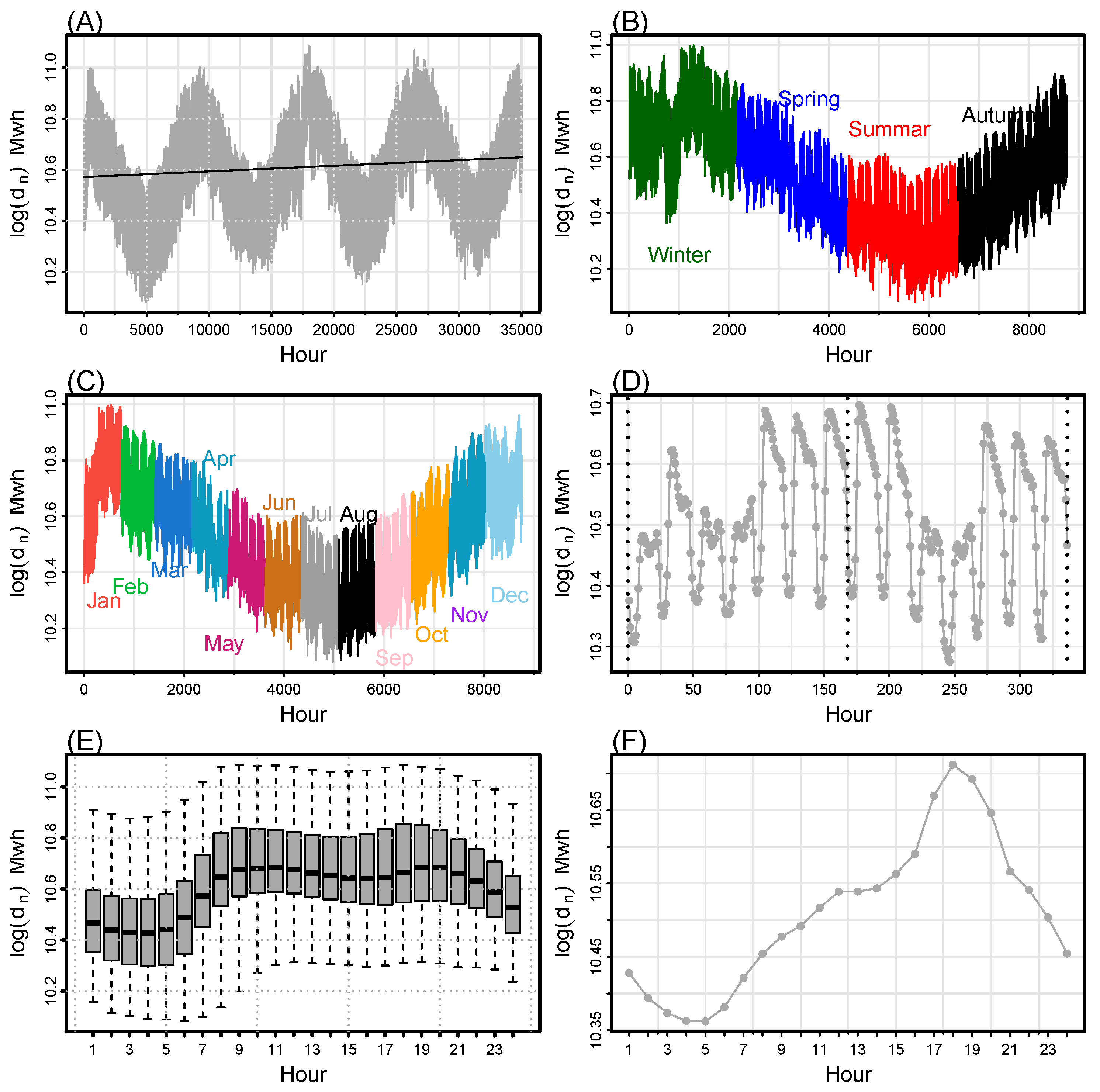
In competitive energy markets, electricity demand time series are characterized by long-term linear (or non-linear) trends, various periodicities (yearly, seasonal, weekly, or daily), non-constant mean and variance, jumps or peaks (extreme values), high volatility, calendar effects, and a tendency to return to average levels. For example, a linear trend and the annual periodicity can be observed in
Figure 1 (A), as well as seasonal variation of the electricity demand throughout a year (B), the monthly consumption of electricity demand (C), the weekly and daily electricity demand patterns (D), the box plot for 24 h (E), and the daily hourly pattern (F). The weekly period includes relatively less volatility in the electricity demand time series. Load profiles vary considerably depending on the day of the week, and demand fluctuates throughout the day. Weekdays have more demand than weekends. In addition, electricity demand is affected by time (extended weekends and holidays) and seasonal effects. However, electricity demand for holidays and long weekends (one day between two non-working days) is significantly lower. Likewise, a variety of environmental, topographical, and climatic factors have a direct influence on the time series of electricity demand [
8].
In order to capture the specific features of the electricity demand time series mentioned above, researchers have proposed various methods and models for the forecast of electricity demand over the past three decades [
9,
10,
11,
12,
13,
14,
15,
16,
17,
18,
19]. Typically, these forecasting methods and models can be roughly divided into three categories: statistical methods, machine learning methods, and hybrid models.
In the first category, generally, the statistical forecasting methods are classified into the following types: parametric and nonparametric regression, linear and non-linear time series, Kalman filters, and exponential smoothing models [
20]. Parametric and nonparametric regression models include polynomial, sinusoidal, smoothing spline, kernel, and quantile regression. Linear and non-linear time series models consider autoregressive moving average, autoregressive integrated moving average, vector autoregressive moving average, and non-linear time series models containing nonparametric autoregressive conditional heteroscedasticity, generalized autoregressive conditional heteroscedasticity, and threshold autoregressive conditional heteroscedasticity [
21,
22,
23,
24]. For example, to forecast one-day-ahead electricity demand, the authors of [
5] used various regression and time series techniques with parametric and nonparametric estimation techniques. They used Nord Pool data on hourly electricity demand to evaluate the proposed forecasting methodology. Based on the empirical results, the proposed component-based estimation method was very effective in power demand forecasting. The proposed forecasting methodology, vector autoregressive modeling combined with spline-function-based regression, performs better than other models. Similarly, exponential smoothing (single, double, and triple Holt–Winter models) is also commonly used to forecast electricity demand [
25,
26,
27,
28]. For example, the authors of [
29] analyzed the parameter space of several seasonal Holt–Winter models applied to power demand in Spain. The authors considered different time frames corresponding to different seasons and distinct training set sizes.
With the rapid development of computational intelligence, machine learning techniques have been extensively applied to different research areas, including short-term electricity load forecasting in the second category. The most commonly used machine learning procedures include artificial neural networks, random forests, deep learning algorithms, decision trees, support vector regression, fuzzy systems, etc. [
30,
31,
32]. For example, the authors of [
33] proposed a deep-learning-based framework for electricity demand forecasting. Cluster analysis was used to transform electricity consumption data into segmented data based on seasons. Based on seasonal, date, and duration data, a multi-input, multioutput short-term memory network model was trained to predict power demand and power consumption data for the Union Chandigarh region of India. Other competitive models were also used in the analysis, such as support vector regression models, artificial neural networks, and neural regression networks. For example, the work reported in [
34] introduced a profile neural network based on convolutional neural networks, which is fast and promising. The developed architecture of deep neural networks was tested on actual electrical data from buildings on a university campus, notably those with high and low levels of seasonal changes. The novel architecture beat current sophisticated deep learning baseline models in prediction accuracy for 1-day and 1-week prediction horizons, improved the average absolute scale error by up to 25%, and improved the training time–accuracy tradeoff.
In the third category, to predict daily electricity demand, many researchers have developed new models by combining the features of two or more models. For instance, the authors of [
35] proposed an adaptive probabilistic and interval forecasting system for multilevel electricity price forecasting. The authors presented two case studies and comparative studies to evaluate the performance of the proposal. The results showed that their proposal would be constructive for electricity market planners. Furthermore, for short-term load prediction, the authors of [
36] introduced a new association model that combines the seasonal autoregressive integrated moving averages and backpropagation neural network models. The outcomes of the empirical analysis showed that the proposed hybrid model obtained highly accurate and efficient forecasts for short-term load forecasting. Similarly, the authors of [
37] showed how to forecast electricity consumption in Turkey using a hybrid model based on the autoregressive integrated moving average model and the least-squares support vector machine model. The results of the proposed approach were evaluated using official forecast data, a single autoregressive integrated moving average model, literature reports, and multiple linear regression approaches. The results show that the model responded better to unexpected responses in the time series.
Another option to enhance performance is to preprocess the original time series data to produce a modified form of the time series that is more reliable [
38,
39,
40,
41]. When predicting energy-related time series, it is common to divide the original dataset into various subseries that may be independently anticipated and averaged to create a real-time time series prediction. The objective is to create a new time series with more or less periodic behavior that is easier to anticipate. This assumption depends on the fact that energy-associated variables are intimately associated with and impacted by climatic and societal factors that exhibit periodic behavior. Thus, to be more correctly anticipated, these subseries must be assigned to specific frequencies embedded in the general behavior of the time series. Empirical mode decomposition and variational mode decomposition are two such approaches, which separate time series into numerous subseries, each with correct oscillation behaviors. Both techniques have been used in a variety of forecasting tools, including autoregressive integrated moving averages, convolutional neural networks, multilayer perceptron, support vector regression, and long short-term memory models [
42,
43,
44,
45]. For instance, the authors of ref. [
46] proposed a “decompose-predict-reconstruct” forecasting model based on empirical modal decomposition and a long short-term memory model. The proposed model effectively improved the load forecast’s efficiency and accuracy. Thus, as reported in these studies, preprocessed models outperform unprocessed models, demonstrating the beneficial effects of including pretreatment in predictive models, representing a fundamental step in the forecasting process because, as proven by previous studies, the performance of forecasting tools improves when correctly chosen and applied to the time series to be forecast.
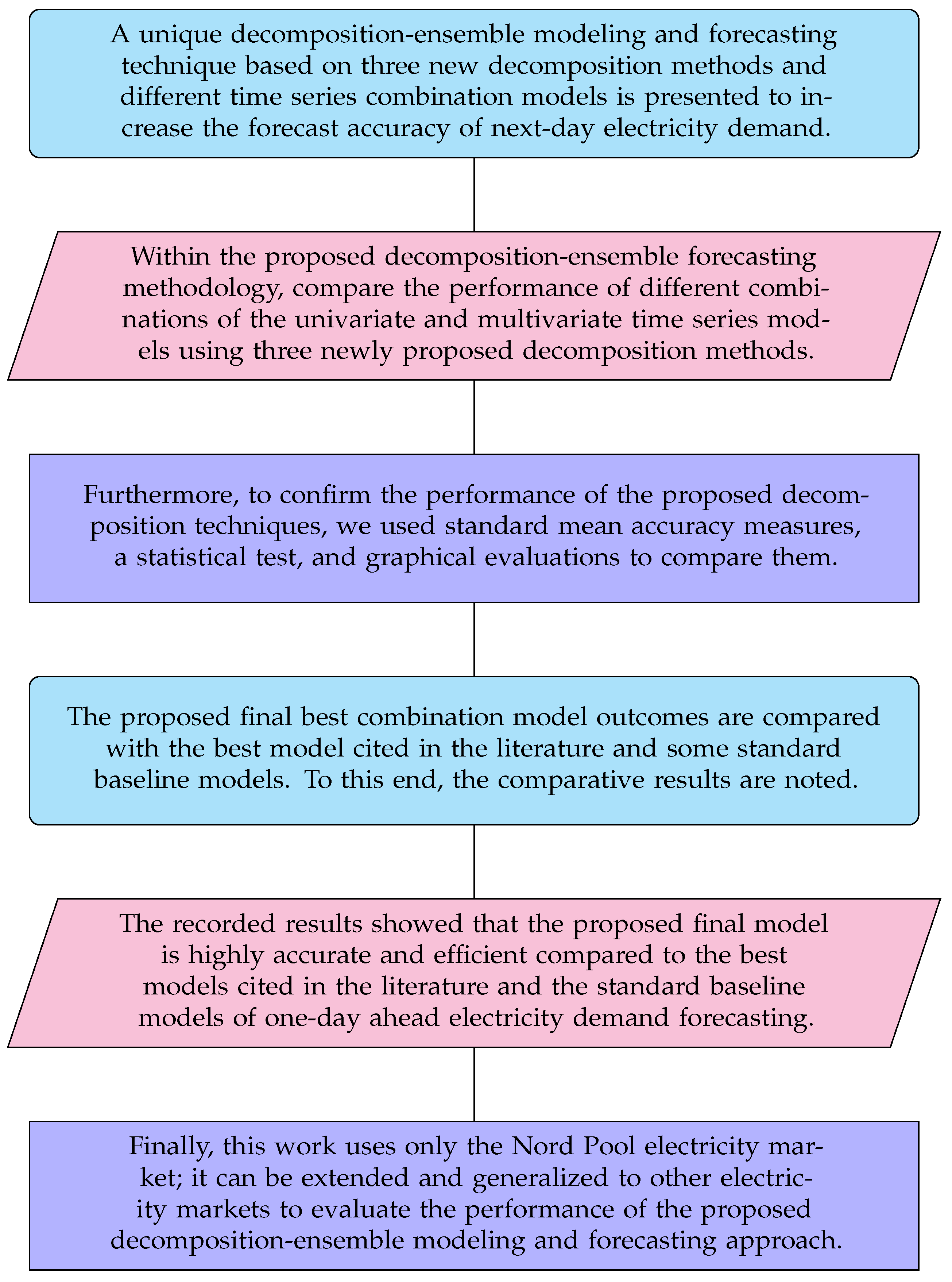
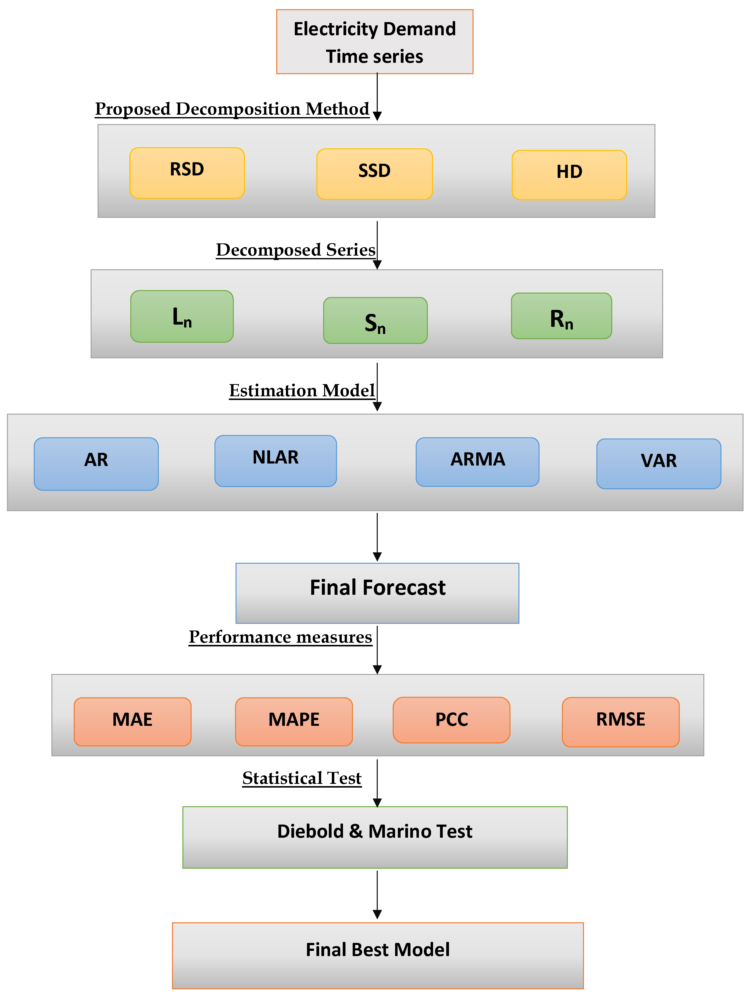
Motivated by the abovementioned works, in this paper, we propose a novel decomposition combination modeling and forecasting framework that is relatively simple and easy to implement and that boosts the forecasting accuracy of short-term electricity demand. The proposed forecasting technique is built on the basis of a combination of unique proposed decomposition methods and traditional time series models. The proposed forecasting technique consists of the following steps. First, using the three novel decomposition methods, i.e., regression spline decomposition, smoothing spline decomposition, and hybrid decomposition methods, the hourly time series of electricity demand is divided into new subseries, namely the long-run trend series, a seasonal series, and a stochastic series. The decomposed subseries are then predicted using four well-known time series models (three univariate and one multivariate), namely linear autoregressive, non-linear autoregressive, and autoregressive integrated moving averages, as well as vector linear autoregressive and all conceivable combination models. As a result, separate predictive models are immediately merged to provide final forecasts a day ahead for electrical demand. The contributions of this work are summarized in
Figure 2.
The rest of this document is formatted as follows.
Section 2 describes the general steps of the proposed decomposition combination modeling and forecasting approach.
Section 3 presents an experimental application of the proposed decomposition combination framework using Nord Pool hourly electricity demand data.
Section 4 provides a detailed discussion of the proposed combination model versus the considered baseline models, including standard univariate and multivariate time series models with and without deterministic components. Finally,
Section 5 discusses conclusions, limitations, and directions for future research.
3. Case Study Outcomes
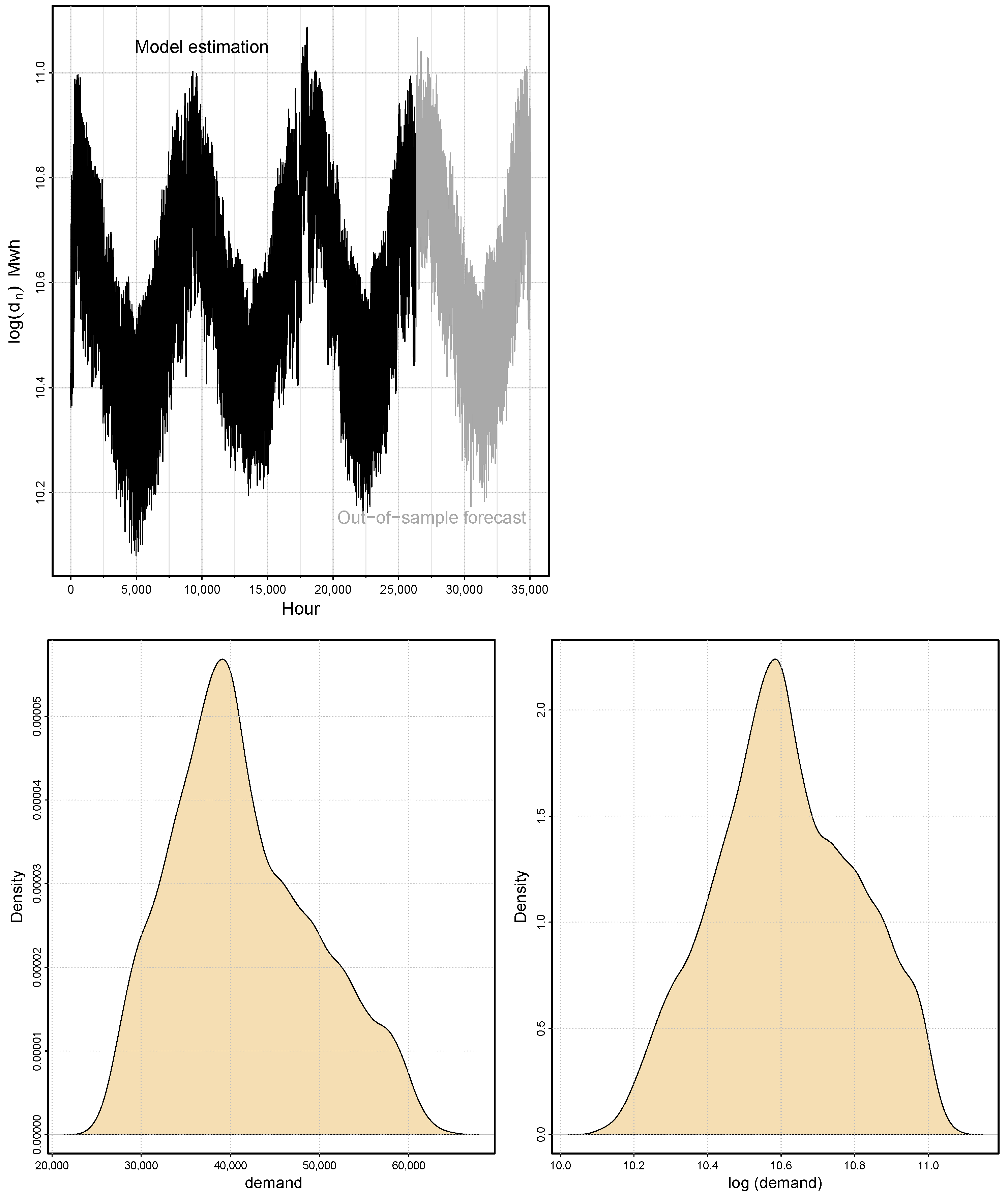
This research work primarily focuses on fluctuations in electricity demand before COVID-19. For this purpose, this work uses the hourly electricity demand (MWh) according to six years of data from the Nordic electricity market collected from 01.01.2014 to 12.31.2019. Each day consists of twenty-four data points, with each data point corresponding to a load period. Therefore, the dataset contains 52,584 data points (2191 days). For modeling and forecasting purposes, we split the data into two parts: a training part (model estimation) and a testing part (out-of-sample forecast). The training part comprised the first five years of data from 01.01.2014 to 12.31.2018 (1826 days or 43,824 observations), spanning five years and accounting for approximately 80% of the total data, with a period of a complete year from 01.01.2019 to 12.31.2019 (365 days or 8760 observations) used for the out-of-sample forecast. Graphical representations of model training and model testing are shown in
Figure 5 (top). Moreover, the density plots for the hourly demand time series and log hourly demand series are shown in
Figure 5 (bottom right) and
Figure 5 (bottom left), respectively. The descriptive statistics of the hourly time series of electricity demand are listed in
Table 1, where the maximum value is 65,311, and the minimum value is 24,739. However, the log demand series and the series without log demand present significant differences, as confirmed by
Table 1.
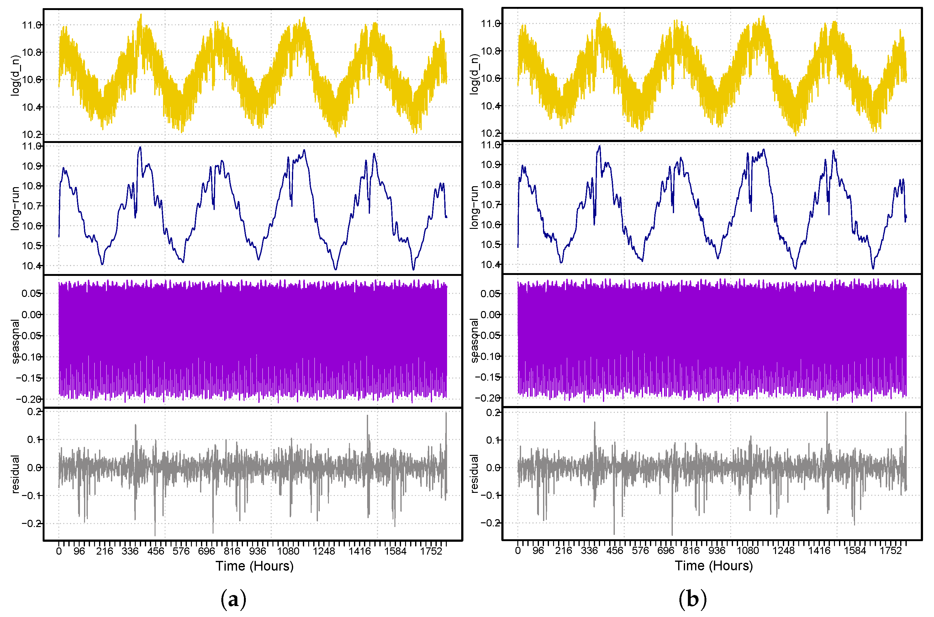
The following procedures must be taken into account in order to produce a day-ahead forecast of electricity demand using the proposed decomposition combination modeling and forecasting technique. To stabilize the variance of the electricity demand time series, the first natural logarithmic transformation was applied. Second, we used the three proposed decomposition techniques to develop temporal subseries for the linear long-term (
), seasonal (
), and stochastic (
) series. Third, each subseries was subjected to the previously discussed univariate and multivariate models. As a result, the models were estimated using a rolling window technique to achieve a forecast for 365 days (8760 data points). For this purpose, Equation (
8) was used to calculate the final one-day-ahead demand forecast. The models’ performances were then evaluated and compared using the MAPE, MSPE, PCC, and RMSE performance metrics, as well as a statistical test (DM test).
Three proposed decomposition techniques were used in this work when decomposing the hourly electricity demand time series (
) into three new subseries: a linear long-term (
), seasonal (
), and stochastic (
) subseries. Four distinct univariate and multivariate time series models were used to forecast these subseries. For univariate and multivariate models, three main combinations are possible: univariate–univariate, univariate–multivariate, and multivariate–multivariate. Combining the models for the subseries estimates led us to compare sixty-four
= 64) combinations for each presented decomposition technique, corresponding to a total of 192 (192 =
) models for the three presented decomposition techniques (SSD, RSD, and HD). The out-of-sample predictions for one-day-ahead accuracy metrics (MAPE, MSPE, PCC, and RMSE) for these 192 models are presented in
Table 2,
Table 3 and
Table 4. The combined univariate–multivariate models outperform the univariate–univariate and multivariate–multivariate models according to the performance metrics. Although multivariate–multivariate combination models produced smaller forecast errors than univariate–univariate models, the mean errors are still larger than those of univariate–multivariate models. In addition, the
SSD
model is confirmed to provide better predictions than all other combination models using the SSD decomposition technique. The best forecasting model (
SSD
) achieved values of 2.028, 0.072, and 0.985 1037.4010 for MAPE, MSPE, PCC, and RMSE, respectively. The
SSD
,
SSD
, and
SSD
models gave the second, third, and fourth best results within all combination using the SSD method. Using the RSD decomposition method, the combined prediction model (
RSD
) achieved the lowest prediction errors, with values of 1.974, 0.068 0.986, and 1081.6590 for MAPE, MSPE, PCC, and RMSE, respectively, with the second, third, and fourth best results achieved by the
RSD
,
RSD
, and
RSD
models, respectively. On the other hand, the combined forecasting model (
HD
) achieved the lowest prediction errors using the HD decomposition method, with values of 1.908, 0.063, 0.989, and 994.1642 for MAPE, MSPE, PCC, and RMSE, respectively. The second, third, and fourth best results were achieved by the
HD
,
HD
, and
HD
models, respectively, within all combination models using the HD method. Among all 192 models, the
HD
model achieved the best forecast using the three decomposition approaches (SSD, RSD, and HD). Based on these conclusions, it is confirmed that univariate–multivariate combinations achieve more accurate predictions competitive model combinations. In addition, the HD decomposition method achieved the lowest mean error among the proposed decomposition methods.
Among the three proposed decomposition techniques, the best four combination models from each decomposition technique were chosen and compared. The mean performance metrics are listed in
Table 5. The
HD
model produced the optimal accuracy metric values (MSPE = 0.063, MAPE = 1.908, PCC = 0.989, and RMSE = 1037.4010) when comparing the results of this model with those of the best remaining model using the proposed decomposition method. Based on the results presented above, we found that the RSD method has the highest prediction accuracy among the proposed decomposition methods.
Once the performance of the proposed best model was determined according to mean accuracy errors, in the next stage, the Diebold and Mariano (DM) test [
48] was used to examine the importance of the differences in prediction abilities between these models. The DM test is a statistical approach widely used in the literature to evaluate predictions from two models [
49,
50,
51]. As a consequence,
Table 5 shows a DM test on each pair of models to confirm the superiority of the model outcomes (mean performance measure). The DM test results (
p values) for day-ahead out-of-sample metrics for the best twelve models are shown in
Table 6. All twelve models listed in
Table 5 are statistically significant at the 5% significance level, while using the HD method, the best four models have high
p values compared to the two other proposed decomposition methods. Therefore, according to the accuracy mean errors and a statistical test, we confirm the superiority of the HD model.
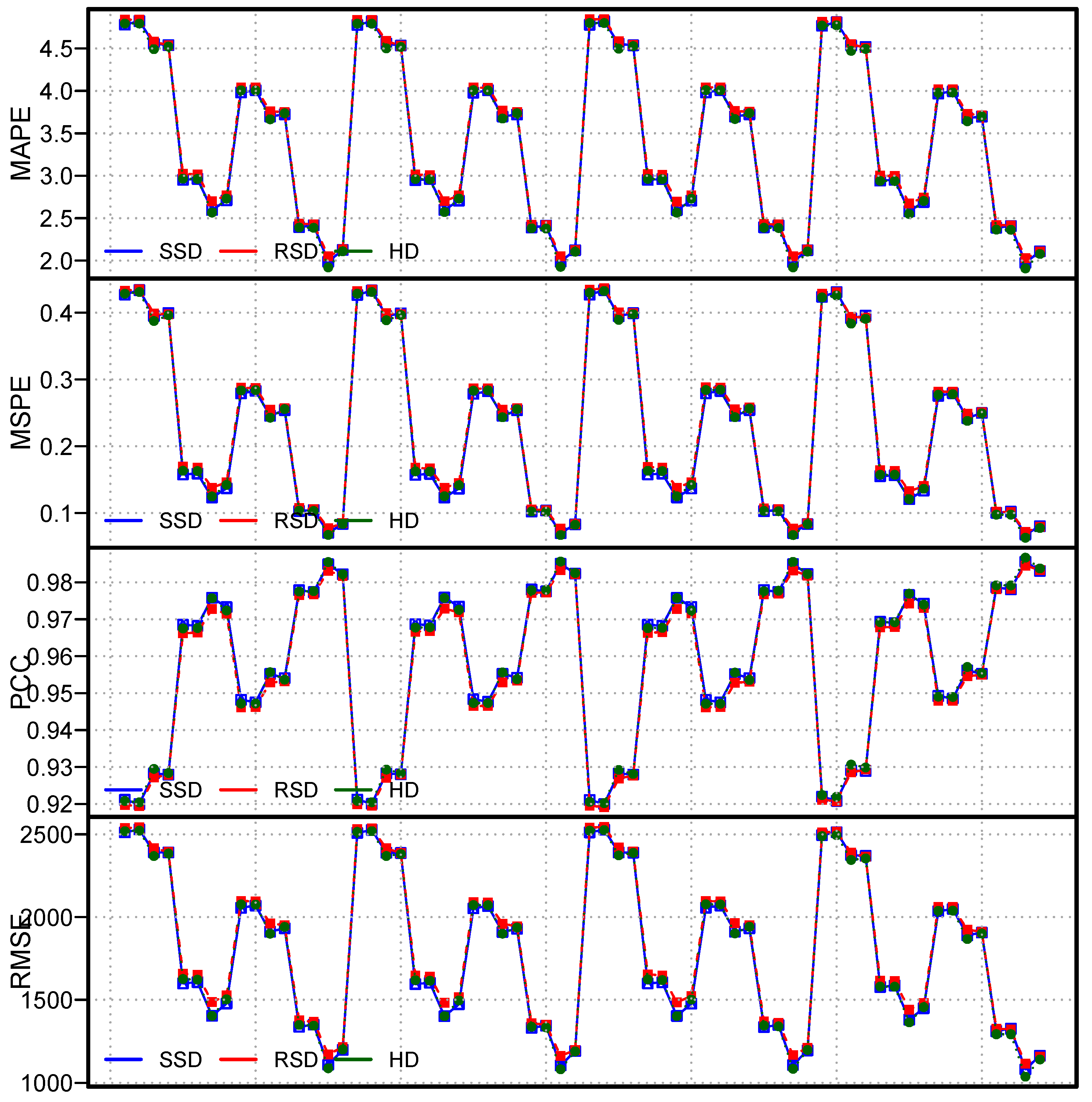
Once the models were tested using the accuracy metrics (MSPE, MAPE, PCC, and RMSE) and a statistical test (the DM test), a graphic analysis was conducted. For instance, a graphical representation of the MSPE, MAPE, PCC, and RMSE for all one hundred and ninety-two models is presented in
Figure 6.
Figure 6 shows that the lowest mean error and the highest PCC values were produced by the
SSD
models, and the
SSD
,
SSD
, and
SSD
models produced the second, third, and fourth best results using SSD method, respectively, while the lowest mean errors and highest Pearson correlation coefficient (MAPE, MSPE, PCC, and RMSE) values were obtained by the
RSD
,
RSD
,
RSD
, and
RSD
models (
Figure 6). In the same way, the lowest mean errors and highest correlation coefficient (MAPE, MSPE, PCC, and RMSE) values were obtained by the
HD
,
HD
,
HD
, and
HD
models (
Figure 6).
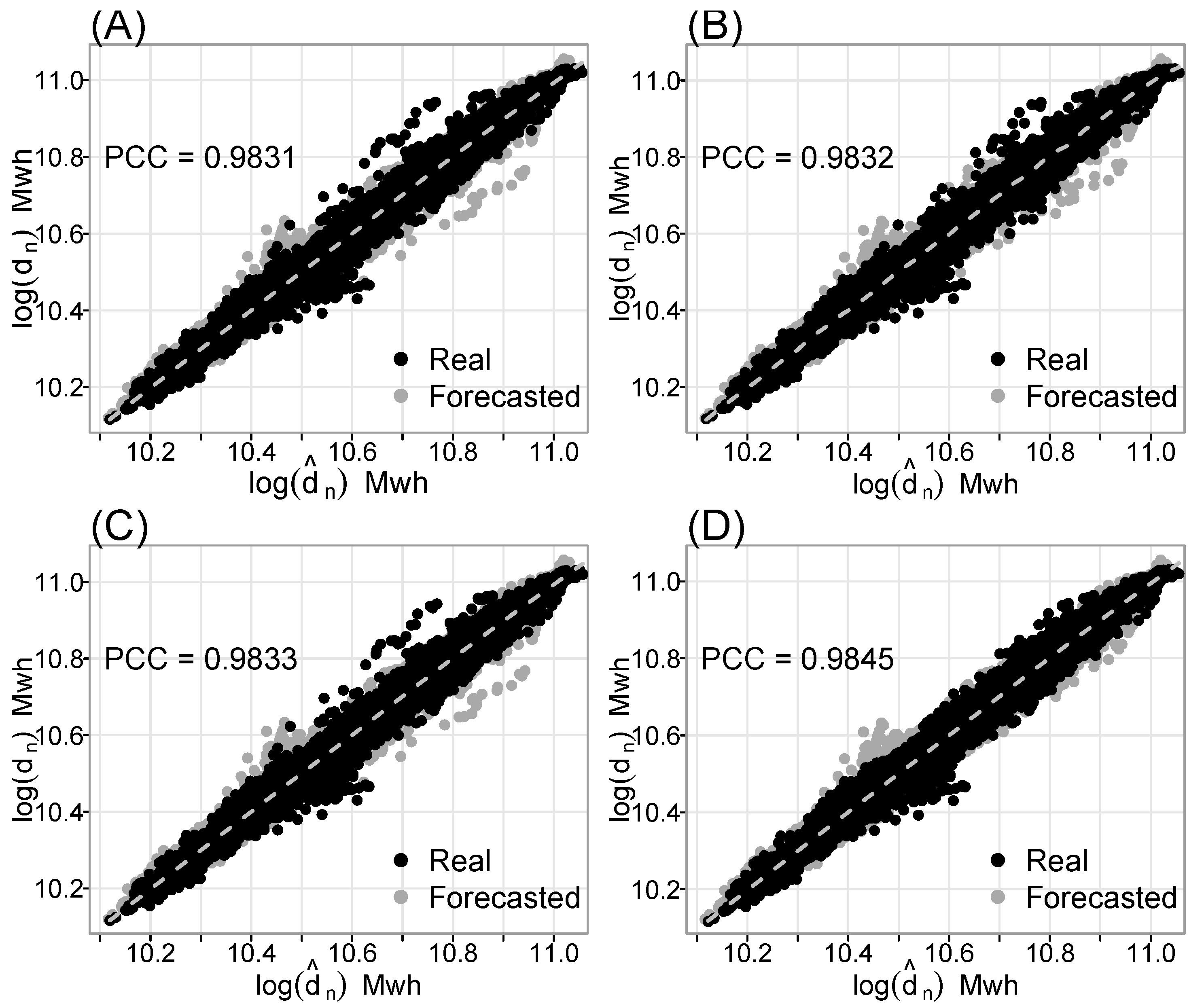
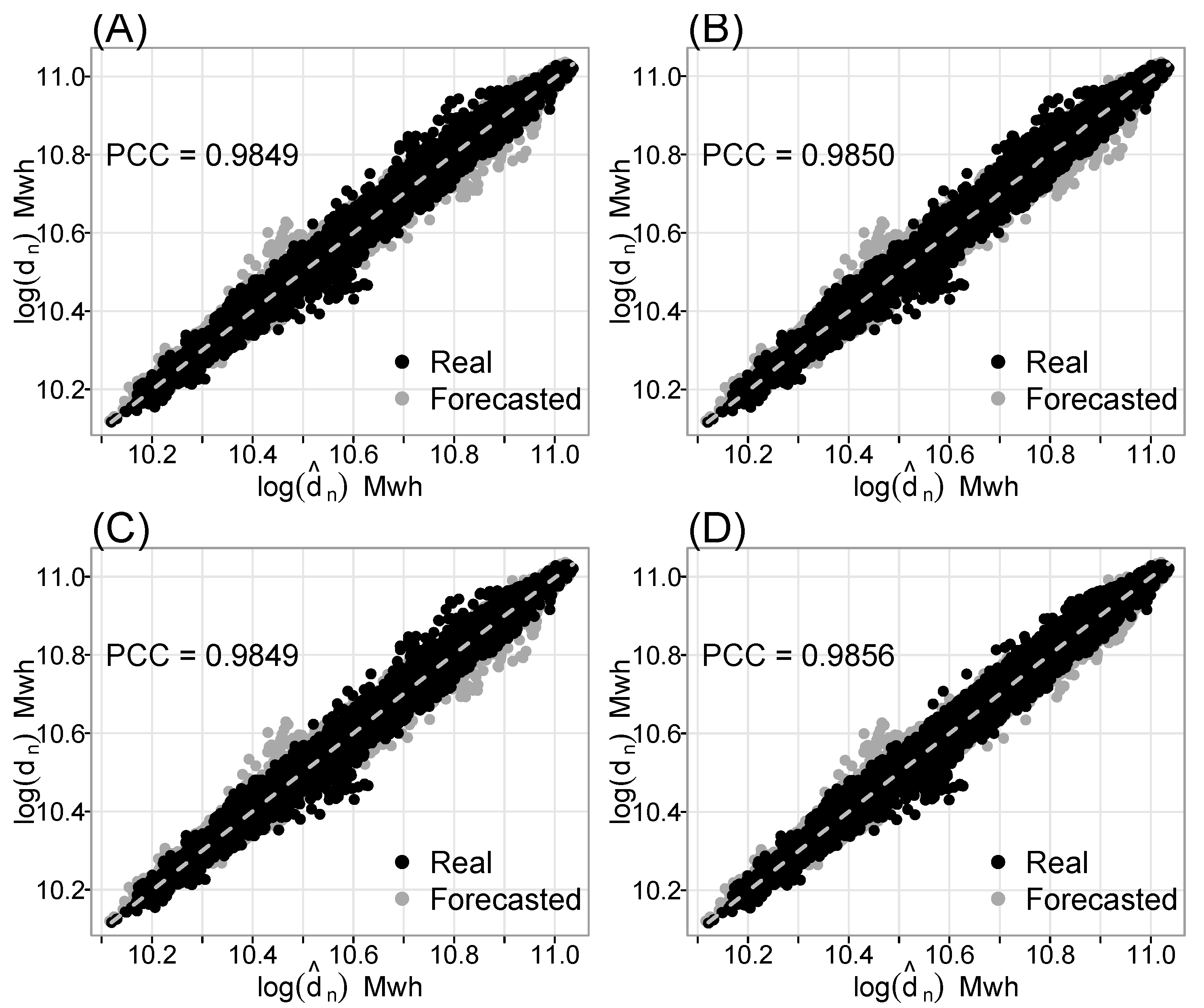
On the other hand,
Figure 7,
Figure 8 and
Figure 9 show the scatter plots of the twelve best models (four for each decomposition approach), as well as their PCC values.
Figure 7,
Figure 8 and
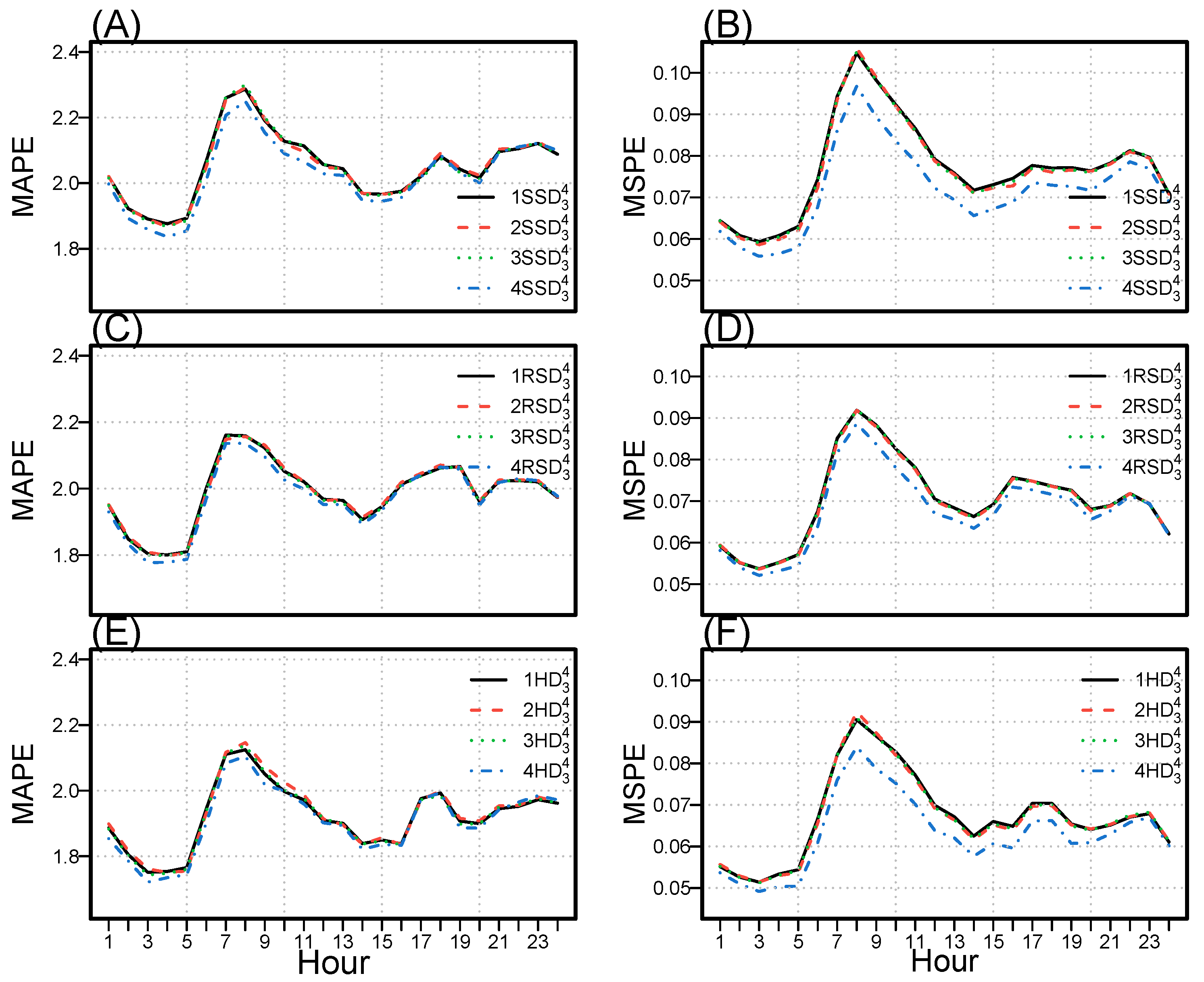
Figure 9 illustrate that the best models have the largest PCC values, with a substantial correlation between actual and predicted values. Furthermore, the hourly MAPE and MSPE for the twelve best models determined using the proposed decomposition techniques (SSD, RSD, and HD) are plotted in
Figure 10 for MPAE (A, C, and E) and MSPE (B, D, and F). The mean hourly errors are lower during the starting hours of the day and slowly increase, with the first peak around 8:00 a.m. After the first peak, the mean error values monotonically decrease, then gradually increase, with the second peak around 4:00 p.m. Finally,
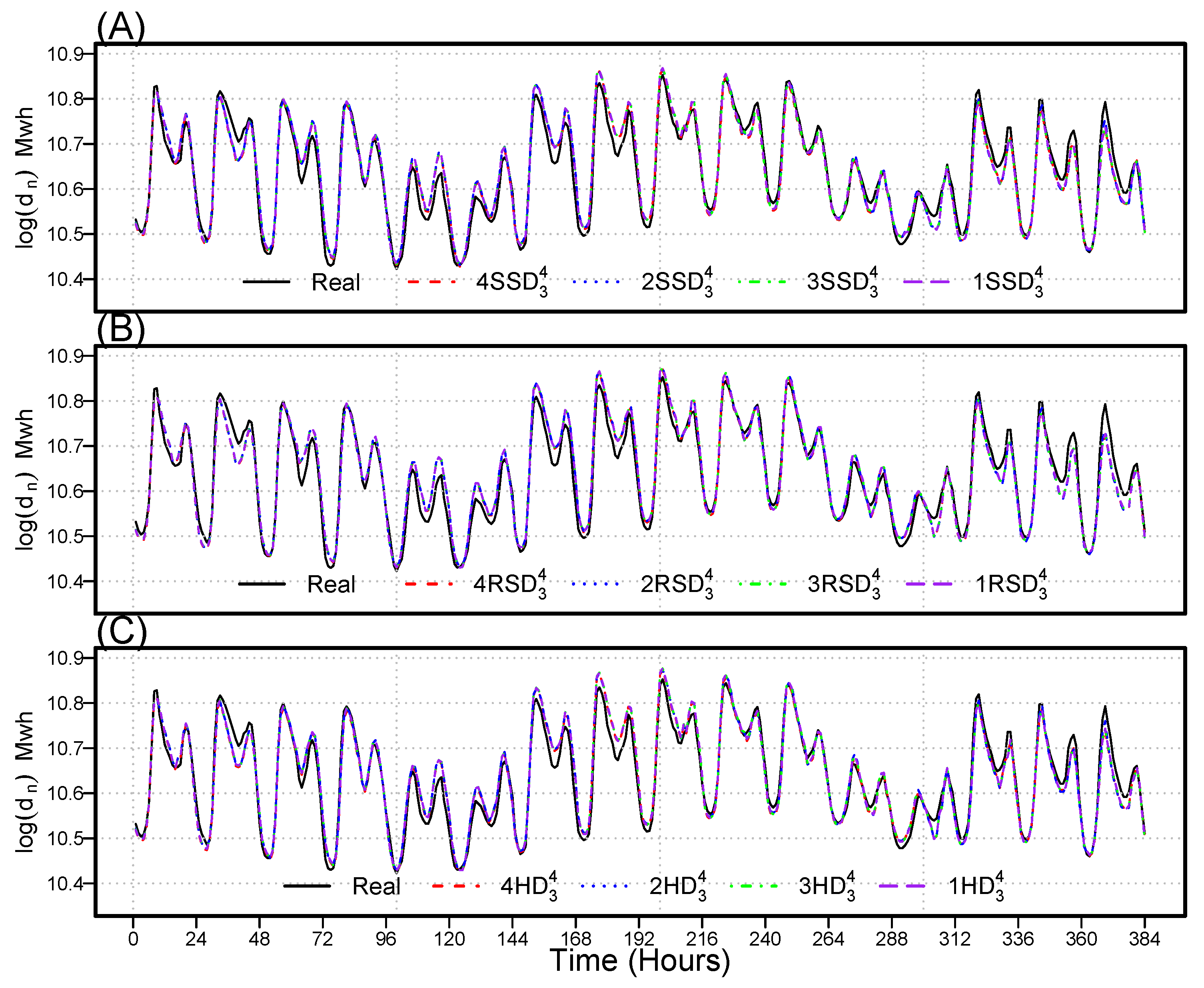
Figure 11 depicts the original and forecasted values for the twelve best models. According to this visualization, the best models’ forecasts closely match observed demand. In addition, this figure confirms that the weekly period includes relatively less volatility in the electricity demand time series, load profiles vary considerably depending on the day of the week, and demand fluctuates throughout the day. Weekdays have more demand than weekends. Therefore, we can determine that the twelve best models outperformed all others of the one hundred and ninety-two models. Finally, based on these descriptive and graphical results, we conclude the univariate–multivariate combined forecasting models achieve the least forecasting errors relative to their counterparts.
4. Discussion
In this section, we compare the results of the best combination model identified in this study with those reported in the literature, as well as those of considered benchmark models. We found our model to be highly comparable with the considered methods.
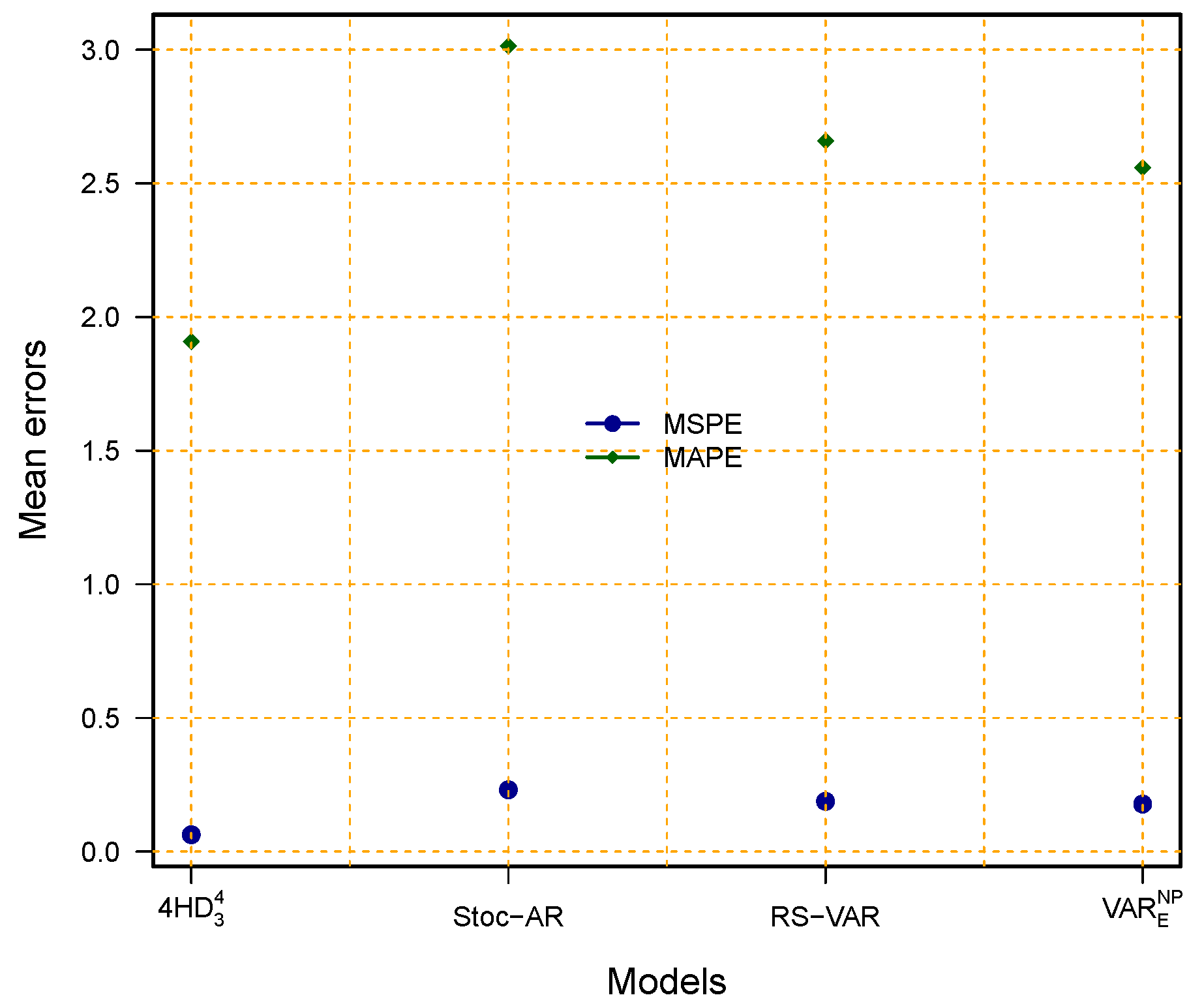
Table 7 and
Figure 12 show numerical and graphical comparisons of the best (
HD
) model identified in this study with the models proposed by other researchers in the literature. Our best (
HD
) model produces the smallest mean errors and the highest correlation coefficient (MSPE = 0.0630, MAPE = 1.9082, RMSE = 1037.401, and PCC = 0.9867) in comparison with the best models reported in the literature. For instance, the best stochastic autoregressive (Stoc-AR) proposed in [
52] was applied to the dataset used in this study, and its accuracy measure (MSPE = 0.2310, MAPE = 3.0134, PCC = 0.9491, and RMSE = 2845.412) was determined and found to be significantly greater than that of our best (
HD
) model. The best model proposed in another study (see [
5]), the regression spline vector autoregressive (RS-VAR) model, was applied to dataset used in the present study and obtained mean errors and Pearson correlation coefficients (MSPE, MAPE, PCC, and RMSE of 0.1878, 2.5587, 0.9622, and 1245.32, respectively) that were also relatively higher than those of our best (
HD
) model. Similarly, in reference [
3], the best proposed nonparametric vector autoregressive model with an elastic net component (VAR
) applied to working dataset used in the present study obtained performance metrics (MSPE = 0.1778, MAPE = 2.5587, PCC = 0.9702, and RMSE = 1207.53) worse than those obtained with our best combination model (
HD
). In this sense, we conclude that the best final model (
HD
) in this study showed high efficacy and high accuracy compared to the best models reported in the literature.
Furthermore, to assess the performance of our best combination model (
HD
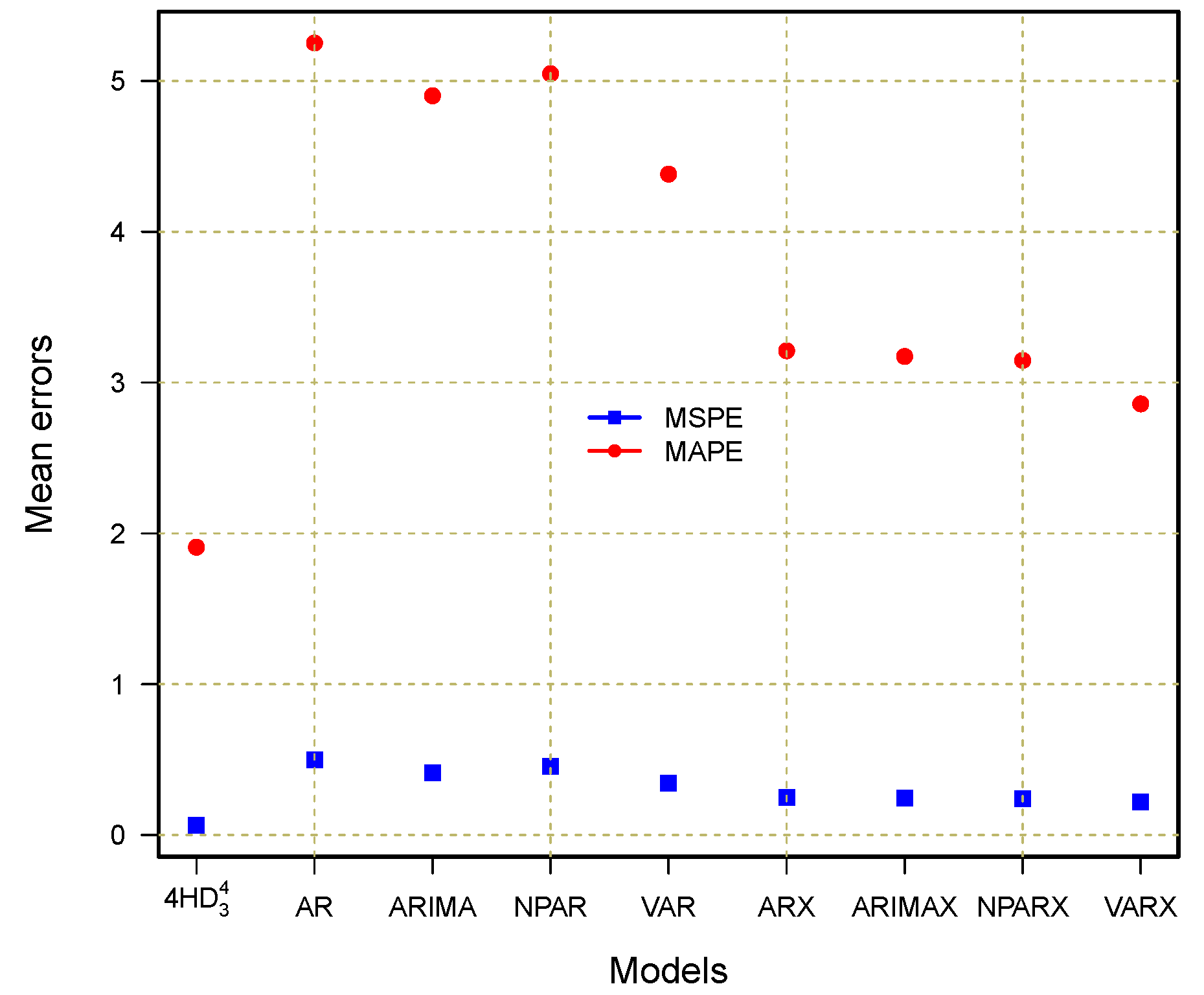
), we also compared it with different standard benchmark models, including the autoregressive (AR), nonparametric autoregressive (NPAR), autoregressive integrated moving average (ARIMA), and vector autoregressive (VAR) models, all of which either included or exclude a deterministic component. In the deterministic component, we included a linear or non-linear long-run trend and yearly, quarterly, and weekly periodicities. Thus, we considered models without deterministic components, such as AR, ARIMA, NPAR, and VAR, as well as models with deterministic components, such as AR-X, ARIMA-X, NPAR-X, and VAR-X. The numerical and graphical comparison results are presented in
Table 8 and
Figure 13, respectively. Within the non-deterministic component models, the VAR model produces the best results (MSPE = 0.3425, MAPE = 4.3823, PCC = 0.9492, and RMSE = 1567.987). When comparing this best model reported in the literature to our best model ((
HD
)), the
HD
model shows significant accurate and efficient outcomes (MSPE = 0.0630, MAPE = 1.9082, PCC = 0.9867, and RMSE = 1037.401). In the same way, the best outcomes are obtained within the deterministic models by the VAR-X model, such as 0.2178, 2.8587, 0.9522, and 1196.068 for MSPE, MAPE, PCC, and RMSE, respectively. However, when compared to the best combination model (
HD
) identified in the current work, it shows significantly worse results. These comparisons are displayed
Figure 13, confirming the superiority of the best combination model (
HD
) identified in the current work. In summary, the best combination model identified in this work obtained high accuracy compared to all benchmark models.
Overall, based on the comparison results of the best proposed models with those presented in the literature using standard univariate and multivariate time series models with and without deterministic components, the best proposed combination model exhibits high efficiency and high accuracy in forecasting day-ahead electricity demand for the Nord Pool electricity market. Precise and efficient day-ahead load forecasting offers various benefits, including effective short-term strategic planning for decreased operating and maintenance costs, optimized supply and demand management, improved system dependability, and future investments. In addition, day-ahead electric power demand forecasting assists in reducing risks and making effective economic decisions that affect profit margins, revenue, distribution of resources, enlargement potential, inventory accounting, operational expenses, personnel, and total expenditure.
To conclude this section, it is worth noting that all implementations were completed using ’R’, a statistical computing language and environment. The GAM library was used to create decomposition techniques and for modeling and forecasting. The forecast, tsDyn, and vars libraries were used to estimate and forecast univariate and multivariate time series models. Furthermore, all computations were run on an Intel (R) Core (TM) i5-6200U CPU running at 2.40 GHz.
5. Conclusions
In today’s liberalized energy markets, electricity demand forecasting plays an important role in planning of generation capacity and required resources. However, electricity demand time series exhibit unique characteristics that corresponding to linear or non-linear long-term trends, with multiple seasonalities (daily, weekly, monthly, quarterly, and annually), jumps or spikes (extreme values), high volatility, non-constant mean and variance, and effects of public holidays. Thus, including these unique characteristics in the model greatly improves predictive accuracy. In order to achieve this, we first split the hourly electricity demand time series into three new subseries—a linear long-term series, a seasonal series, and a stochastic (irregular) series—using the three proposed decomposition methods: regression spline decomposition, smooth spline decomposition, and hybrid decomposition techniques. Next, to forecast each subseries, we used different univariate and multivariate time series models, including autoregressive, non-linear autoregressive, autoregressive integrated moving average, vector autoregressive, and all feasible combinations thereof. In summary, in this work, we compared three decomposition methods and all their possible combination models with univariate and multivariate models. The individual forecasting models were combined directly to obtain the final result of a one-day-ahead electricity demand forecast. From 1 January 2014 through 31 December 2019, the proposed modeling and forecasting technique was applied to hourly electricity demand based on Nord Pool power market data. Three accuracy measures (MSPE, MAPE, and PCC), a statistical test (the DM test), and graphical representations (line plot, bar plot, correlation plot, and dot plot) were used to validate the performance of the proposed modeling and forecasting framework. The empirical findings indicate that the proposed decomposition combination modeling framework is highly effective in short-term electricity demand forecasting. It is also confirmed that among the proposed decomposition methods, the hybrid decomposition method outperforms the other two proposed methods and increases the performance of final model forecasts. Additionally, our forecasting outcomes are comparatively better than those achieved using methods mentioned in the literature. Lastly, we recommend that the modeling and forecasting approach described in this study be applied to tackle other electrical market forecasting difficulties.
The main drawback of this research is that it only includes hourly electrical demand data, without incorporating additional exogenous factors, such as electricity pricing, temperature, wind speed, natural gas prices, etc., which might enhance day-ahead electricity demand forecasting. On the other hand, in the current work, we used only data from the Nord Pool electricity market. Therefore, the results reported herein can be extended to other electricity markets to evaluate the performance of the proposed decomposition-combination modeling and forecasting approach. Furthermore, since only linear and non-linear univariate and multivariate time series models were used in this work, machine learning models such as deep learning and artificial neural networks can also be considered within the current decomposition combination forecasting framework. It can also be extended and applied to other approaches and datasets (for example, energy [
53,
54,
55], air pollution [
56,
57,
58,
59], solid waste [
60] and academic performance [
61]).
