Charging Scheduling of Hybrid Energy Storage Systems for EV Charging Stations

Abstract

The growing demand for electric vehicles (EV) in the last decade and the most recent European Commission regulation to only allow EV on the road from 2035 involved the necessity to design a cost-effective and sustainable EV charging station (CS). A crucial challenge for charging stations arises from matching fluctuating power supplies and meeting peak load demand. The overall objective of this paper is to optimize the charging scheduling of a hybrid energy storage system (HESS) for EV charging stations while maximizing PV power usage and reducing grid energy costs. This goal is achieved by forecasting the PV power and the load demand using different deep learning (DL) algorithms such as the recurrent neural network (RNN) and long short-term memory (LSTM). Then, the predicted data are adopted to design a scheduling algorithm that determines the optimal charging time slots for the HESS. The findings demonstrate the efficiency of the proposed approach, showcasing a root-mean-square error (RMSE) of 5.78% for real-time PV power forecasting and 9.70% for real-time load demand forecasting. Moreover, the proposed scheduling algorithm reduces the total grid energy cost by 12.13%.

1. Introduction

Transport contributes over 20% of greenhouse gases [1]. Road transport constitutes 77% of overall transport emissions in the European Union (EU) [2]. It makes land-based travel a significant threat to the environment. One of the most planned policies in the transport sector focuses on promoting EV to decrease carbon emissions [2]. With the combined efforts of various policies and initiatives, the global EV fleet of 4 million in 2016 is expected to reach an estimated 70 million by 2025 [3,4]. However, in this new era, the infrastructure needed to support the operation of EV, especially charging stations, has yet to be ready to meet the increasing demand. Moreover, it must be accounted for that most people may not switch to EV just because of the environmental aspect [3]. The main drawbacks of EV are that they need to be charged frequently and have longer charging times [3]. It is necessary to have a fast and cost-effective charging infrastructure to address these drawbacks and enhance the acceptance of EV [3]. However, demand scheduling to achieve a cost-effective solution is challenged due to uncertainty in demand. Hence, demand forecasting is an essential approach to overcoming this problem.

Furthermore, traditional vehicle energy sources are conventional fossil fuels, which combine two crucial negative aspects. They are present on the earth in a limited quantity, and they release greenhouse gases when they are burned [5]. EV provide alternative energy sources with renewable energy sources (RES), which have unlimited availability and emit no greenhouse gases. Thus, it requires the use of RES to have truly sustainable road transport. The extensively adopted form of RES by many countries worldwide is solar power (or PV power) [6]. PV power production is projected to represent approximately 20% to 25% of global generating capacity by 2050 and become one of the fundamental energy sources [7]. Despite the numerous benefits of solar power generation, its integration into the power system faces challenges due to its variable and fluctuating nature, leading to uncertainties within the power sector [8]. To address this challenge and integrate solar energy into CSs, the use of an energy storage system (ESS) is necessary [9]. In terms of efficiency, lifetime, reliability, and economic viability, the synergistic combination of different ESSs, called hybrid energy storage systems (HESS), outperforms a single ESS, demonstrating enhanced overall performance [10], thus being more suitable for large-scale RES systems. In order to have a flexible and smart management of HESS, forecasting upcoming solar energy generation and load demand is required [11].

Recent studies provide valuable insights into potential solutions in this domain. For the sake of comprehensiveness, related research in ESSs and HESS is briefly mentioned, and we examine their characteristics, advantages, and disadvantages. HESS offer a novel way to boost the resilience and reliability of renewable energy (RE) systems, as they merge the advantages of various energy storage technologies [12]. Nevertheless, designing an ideal HESS is challenging due to the complexities of system design, simulations, and optimization techniques. Selecting the best hybridization and control strategies also poses challenges, primarily due to a lack of industry standards and practical issues such as high costs, short lifespan, and emissions [13]. One of the most recently used ESSs in HESS is the redox flow battery (RFB) known for its high capacity and long life [13].

HESS technology faces multiple optimization problems, i.e., sizing, capacity, and power distribution, since it is still an emerging technology. Thus, several optimization techniques such as genetic algorithms (GA) and ant colony optimization (ACO) were adopted in the literature to fix these issues (see

Table 1. Recent studies on optimization techniques.

Ref.	Optimization Technique	Objectives	Constraints	Pros	Cons
[14]	AI-based optimization	Optimize EV charging in PV-powered stations	Accurate prediction of PV power, charging station capacity	Cost reduction, grid load management	Implementation complexity, limited consideration for grid constraints, and user behavior assumptions.
[15]	Mixed-integer linear programming (MILP)	Efficiently manage energy resources, and cost minimization	Charging and discharging power limits, battery SOC constraints	Cost optimization, realistic representation	High computational resources
[16]	Ant colony optimization (ACO)	Optimizing RES usage and electricity purchasing	Battery SoC limits	Low purchasing cost	N/A
[17]	Genetic algorithms (GA) and dynamic programming (DP)	Optimize the charge/discharge schedules of ESSs to minimize electricity expenses	ESS capacity, charge/discharge limit	Flexibility	Computational complexity, dependency on accurate prediction.
[18]	Particle swarm optimization (PSO)	Optimize battery energy control in a grid-connected microgrid to reduce electricity costs	battery SoC limits, charging and discharging rate	Real-time energy management, a dynamic penalty function	The algorithm’s effectiveness depends on the choice of parameters such as population size, inertia weight, and learning factors.

N/A: not available

) [14,15,16,17,18]. In [14], the authors propose an optimal charge-scheduling algorithm for EV based on day-ahead PV power forecasts in order to minimize the total charging costs. In [15], an optimization model and energy management schemes for microgrids to increase the efficiency of EV are suggested. In [16], the authors propose a 24-h-ahead operational timeline at an hourly resolution model, integrating RE to minimize costs. In [17], the authors propose a combination of genetic algorithms (GA) and dynamic programming (DP) to create charge/discharge schedules for ESSs within the context of time-of-use pricing and RE integration. In [18], the authors present real-time energy management for optimally managing battery charging/discharging operations in a grid-connected microgrid and minimizing power costs.

Several studies have been conducted on PV power forecasting, and different machine learning (ML) algorithms have been implemented. For example, the authors in [19] found that the use of an LSTM network with a larger number of time steps and a more extensive network was more proficient in capturing long-term trends, outperforming traditional ML models. Meanwhile, in [6], the authors concluded that a univariate model using historical PV power data was sufficient for one-step forecasting, while multistep forecasting required a multivariate model incorporating historical meteorological variables and PV output data. Moreover, the model struggled with fluctuations, indicating optimal performance under stable weather conditions.

Load demand has not been frequently studied in recent years, mainly due to the lack of datasets and more especially real datasets. In [20], the authors constructed models with varying input features, discovering that a model incorporating load demand data, calendar features, and weather features yielded the highest accuracy. However, postprocessing was needed to handle constraints in the data. Meanwhile, the study [21] found that LSTM networks outperformed autoregressive integrated moving average (ARIMA) models for predicting charging loads. The drawback of that study was the lack of data during holidays and semester breaks. Lastly, the paper [22] compared the following algorithms: artificial neural networks (ANN), RNN, gated recurrent unit (GRU), and LSTM, and proved a single-hidden-layer GRU outperformed others in predicting EV load demand and providing insight into weekly consumption patterns.

In this paper, we propose a three-stage-based approach to find an optimal charging schedule for an HESS to achieve a clean, cost-effective, sustainable, and efficient EV charging station. To the best of our knowledge, no comprehensive study in the existing literature has yet considered a multistage approach that addresses the challenges associated with solar energy, demand uncertainty, HESS charging scheduling, and cost reduction simultaneously.

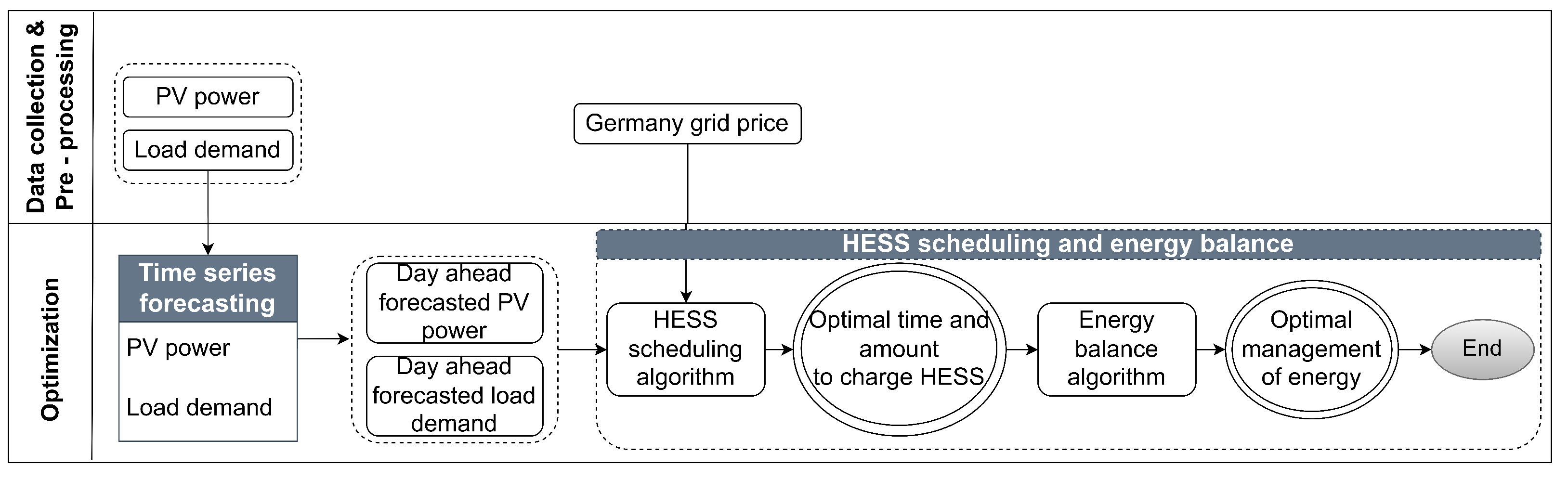
• In the first and second stages, the PV power and load demand are forecasted to provide vital insights into the upcoming energy status for optimal energy management.
• In the third stage, a scheduling algorithm is implemented based on the outputs of the previous stages to predict the best times for charging the HESS, while maximizing the PV power utilization and minimizing the grid energy costs.

The remainder of this paper is structured as follows: Section 2 defines the overall proposed approach. Section 3 is devoted to the PV power forecasting. It starts with the analysis and the preprocessing of the real used PV power dataset. Then, the different adopted DL algorithms are detailed, and their results are discussed. Section 4 is dedicated to the load demand prediction. Multiple DL algorithms were implemented to forecast the load demand in real-time and for the day-ahead, and then the findings were evaluated. Section 5 presents our proposed charging scheduling algorithm. First, the principal is outlined. Then, comprehensive experimental simulations are conducted to analyze several scenarios, for example high demand and high solar power. For each case, three configurations are implemented to assess the performance of our proposal: a baseline configuration (i.e., without predicted data), our proposal, and our proposed algorithm using real data instead of forecasted data. Finally, Section 6 concludes the paper and suggests areas for further research.

2. Proposed Approach

This research is part of the OMEI project (a national German project). The overall goal of this project is to build two distinct EV charging stations. Each charging station contains the following main components, as illustrated in Figure 1:

• A HESS made up of a lithium battery with a capacity equal to 220 kW and a metal-free redox flow battery with a capacity equal to 400 kW. The topology used in our HESS is a DC-DC converter. The battery with a high capacity is mainly used to meet the load demand, and the second battery is used as a support. In our system, the utilization of renewable energy (i.e., especially PV energy) to charge the HESS is a high priority.
• The sources of energy used in our system are PV energy and grid energy. In each charging station, a PV field is built. The grid is used to provide energy to our system when the PV is not sufficient to meet the demand.
• Three charging connectors: these are the terminal connections that are linked to the EV and the charging cable. In our system, we have two fast charging cables and one normal charging cable.

The proposed approach for the optimal charging scheduling of the HESS is illustrated in Figure 2. It is composed of two main steps. First, the prediction of the PV power and the load demand, and second, the determination of the optimal time to charge the HESS based on the forecasted data and the “Germany grid price”, which is the actualized electricity prices for the day-ahead electricity market in Germany.

3. PV Power Forecasting

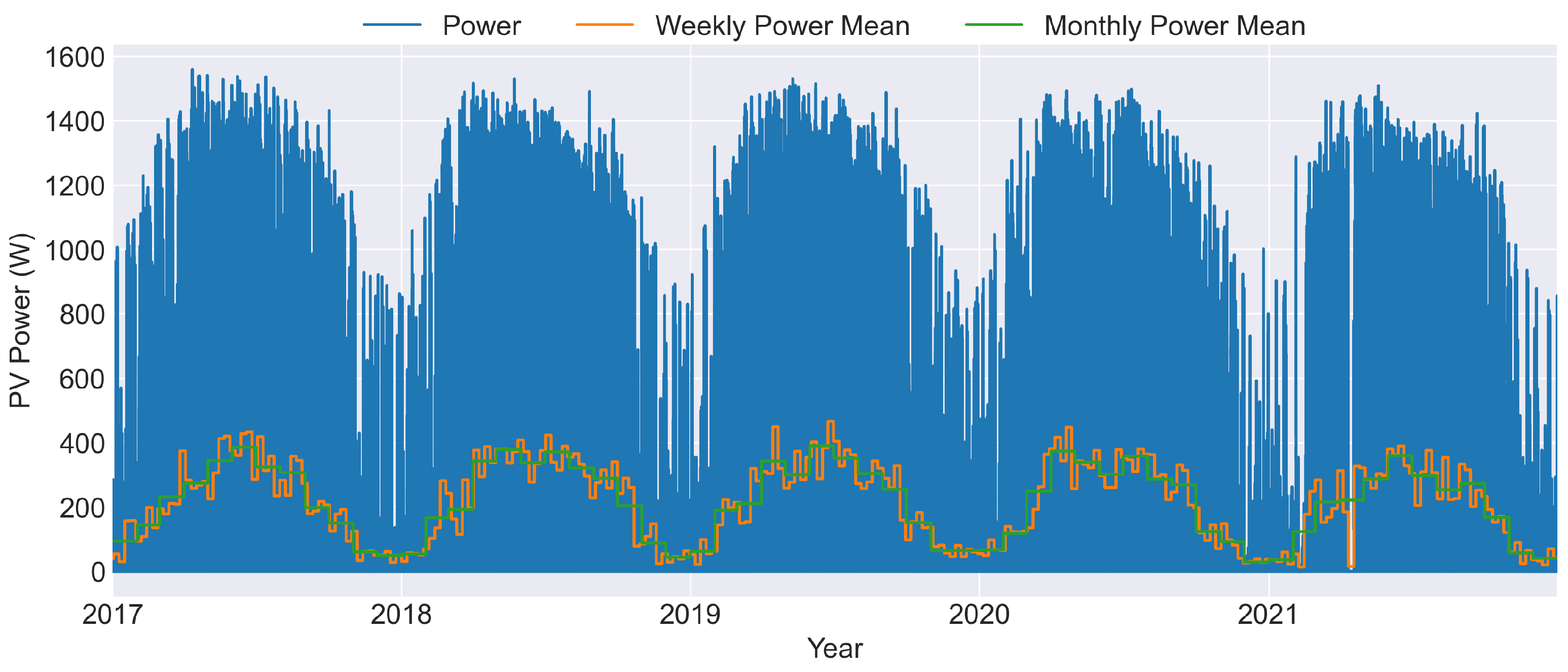
A real dataset was used to forecast the PV power. The forecasting process involved the following steps: data preprocessing, model structure definition, and hyperparameters for training and validation precision. A grid search-based cross-validation was adopted to assess the model performance. Two types of univariate forecasting were used to evaluate our proposal: the first was one-step (15 min, real-time) forecasting, and the second was multistep (one-day) forecasting.

3.1. Data

The real PV dataset was collected from a PV field located in Bavaria, Germany. The dataset included power measurements in watts, recorded every 15 min from 1 January 2017 to 31 December 2021, as highlighted in Figure 3. The plot also includes the mean of the produced PV power, calculated weekly (week of the year) and monthly over time. The yearly periodicity of power generation creates a clear pattern in the plot. This cycle is mainly due to annual changes in the amount of received solar radiation. Typically, PV power generation is the highest in summer and the lowest in winter.

3.2. Data Pre-Processing

The voltage and readings are sensitive owing to the PV characteristic of the solar cell [23]. These solar equipment problems, electrical noise [24], collection system errors, and software system problems may cause certain data outliers. Outliers in a forecasting model might lead to significant forecasting errors. Therefore, data preprocessing is crucial for optimizing training, computing cost, and model correctness [25]. The different preprocessing steps involved were as follows:

• First, duplicate data entries in the dataset, which had the same datetime index and identical power values, were removed from the dataset. Furthermore, the dataset was further analyzed by month and week of the year. During that analysis, outliers were identified and removed. The missing values were estimated using mean imputation [26,27], which employs a time-based average. This approach filled in the missing values by averaging data from the preceding year with a similar date. It was a feasible strategy because of the similar value of PV power generation at the same time intervals over the years.
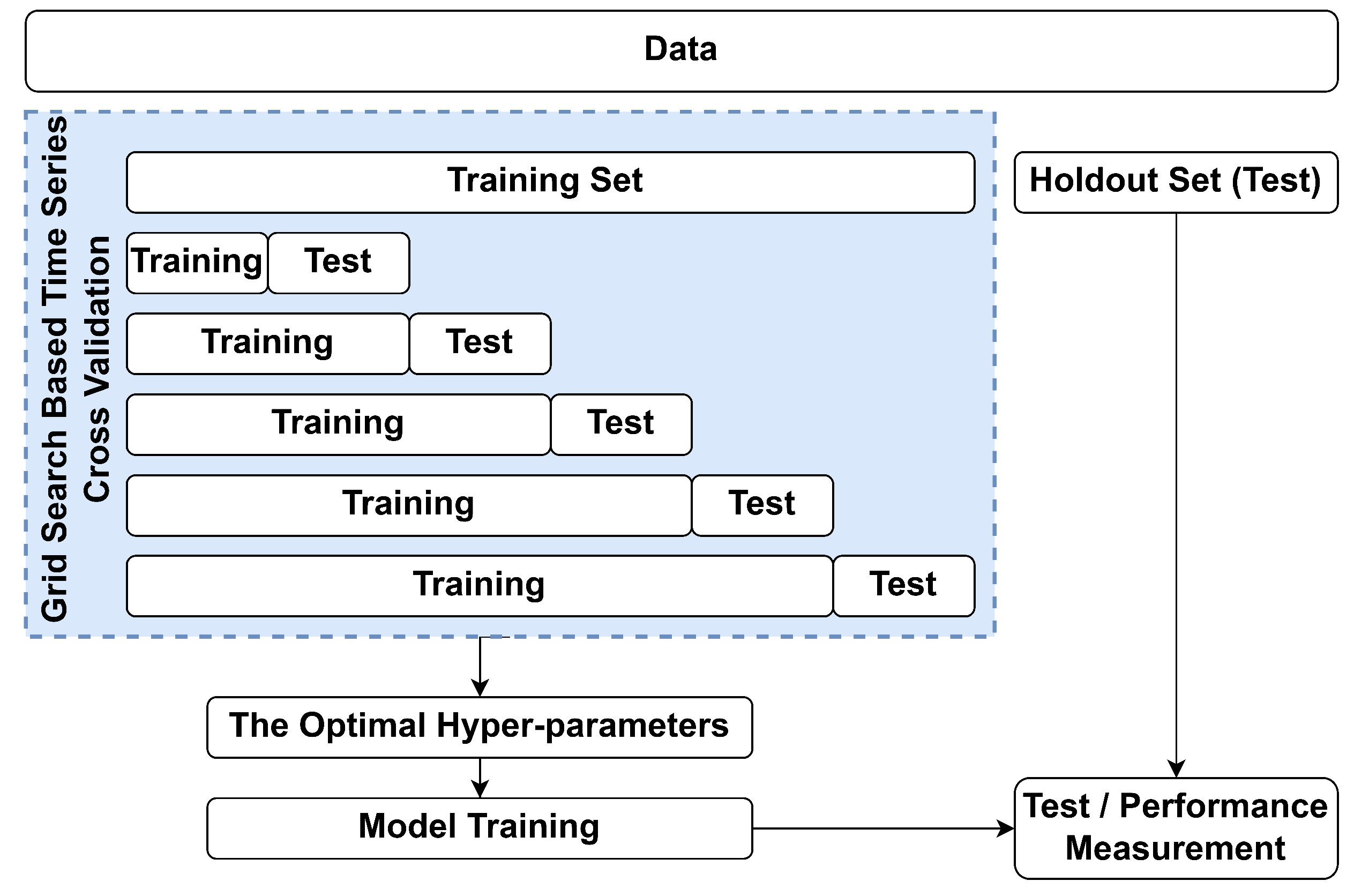
• Second, the dataset was split into a training dataset (80%) and a test dataset (20%). The training set included PV power data at 15 min intervals from January 2017 to December 2020, while the testing set covered January 2021 to December 2021. Additionally, time series cross-validation was implemented during the model training phase to ensure a robust model evaluation and mitigate the risk of bias associated with specific years, such as 2017 or 2021, when external conditions might have influenced patterns.
• Third, two prominent scaling methods, z-score normalization and min-max scaling, were compared using the test dataset [8,19]. The outperforming min-max scaling was utilized. The min-max scaler was fitted using only the training data to prevent data leakage. Using both training and test datasets could introduce reference points from the test set, potentially influencing the values of the training data and causing data leakage [28].
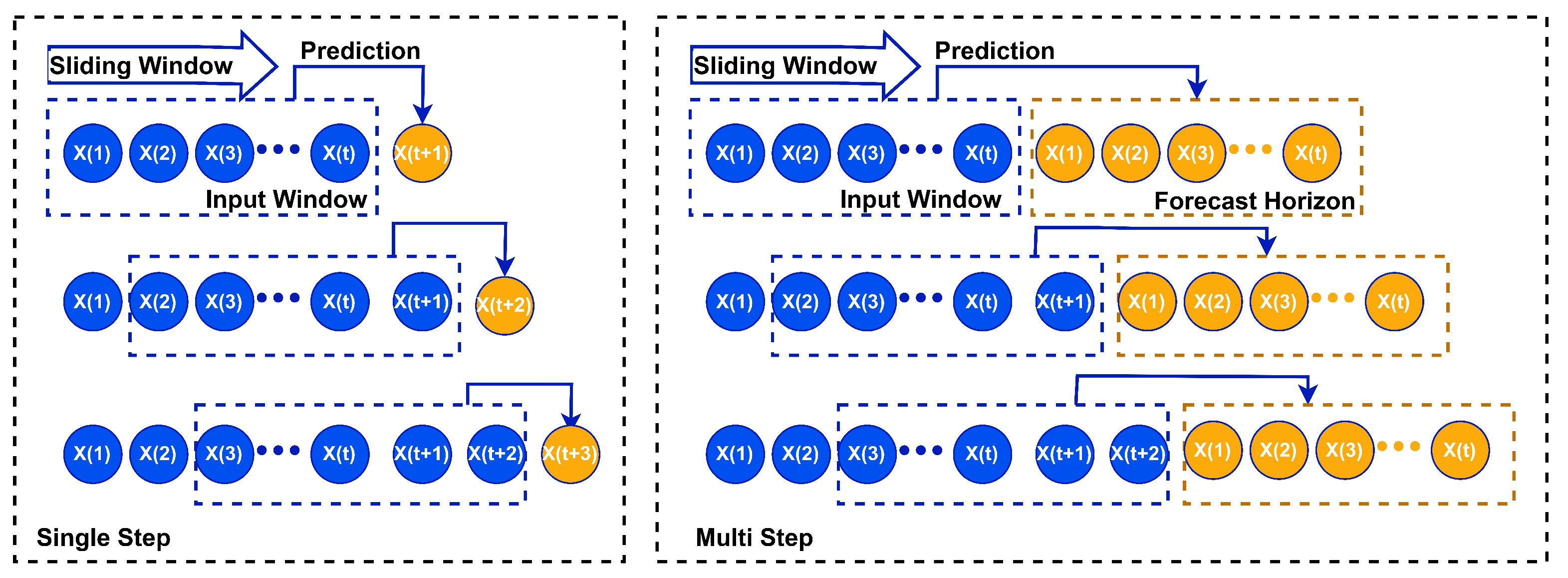
• Fourth, the sliding-data-window approach was adopted to generate input–target pairs [29], thereby framing the forecasting procedure as a supervised learning task [30]. A fixed-size window slid throughout the PV power time series data; the window size was a sliding window specifying the value for the input. The PV power at the forecast horizon was used as the target, as illustrated in Figure 4. In this work, different window sizes for PV power forecasting were examined, and the one with the lowest mean squared error (MSE) was selected. For one-step forecasting, a window size of 96 was selected to predict the horizon number 1. On the other hand, for multistep forecasting, a multi-input multioutput (MIMO) strategy [31] was utilized. A window size of 288 was used with a 96-h forecasting horizon. PV power generation is strongly influenced by daily patterns, such as sunrise and sunset times; by using a daily window size period, the model can capture these daily cycles and learn the underlying patterns in PV power generation.
• Lastly, numerous zero (nighttime) values in the dataset cause data sparsity and make forecasting challenging. Some research handles this data sparsity by working only on daytime values [6,32]. We handled this issue by trying different scaling methods and activation functions. Min-max scaling with a sigmoid activation function on the dense layer of the model further improved the performance in handling night values.

3.3. Model Training and Validation

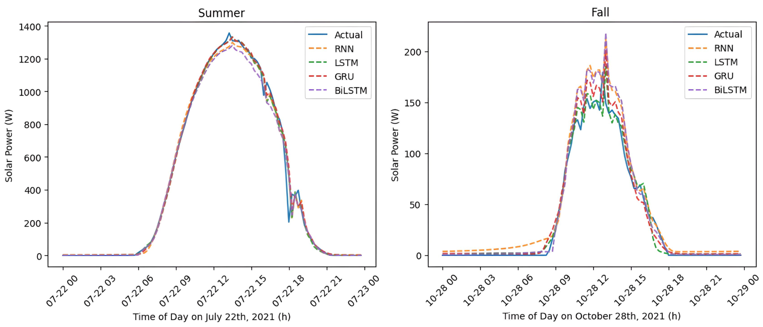
The RNN, LSTM, GRU, and BiLSTM deep learning algorithms were utilized for both one-step and multistep forecasting, while EDLSTM was adopted exclusively for multistep forecasting. RNNs are NNs designed to work with sequential data [33]. They can model temporal behavior and dependencies among data points linked in time or space [34]. However, training an RNN to capture long-term dependencies is difficult due to the exploding and vanishing gradient problems [35]. The LSTM units are designed to address this problem [36]. A GRU has recently followed LSTM as a simpler alternative with fewer parameters [37,38]. These two RNN enhancements were proven to overcome the gradient problem by capturing long-term dependency. The BiLSTM is an extended version of standard LSTM [39]. An LSTM model processes data in only one direction, namely, from the earlier parts of a data sequence to the later ones. BiLSTM simultaneously takes into account data before and after the current point [40]. EDLSTM or sequence-to-sequence (seq2seq) architectures [41] were introduced as an efficient solution for sequence-to-sequence problems [41]. Moreover, many recent research studies have demonstrated the effectiveness of the RNN, LSTM, GRU, BiLSTM, and EDLSTM DL algorithms [13,33,35] compared to traditional ML models [19,42] or statistical models [32] in tasks related to PV power forecasting. In our work, we opted for these algorithms to predict the PV power using the past PV power data. Each deep learning model contains several hyperparameters. The optimal architecture of NNs, including the appropriate number of layers and neurons in each hidden layer, is not dictated by fixed theoretical guidelines but relies on a combination of problem-specific requirements, trial and error, and adaptive learning processes [43]. Hyperparameter tuning was performed to fairly compare architectures and identify the optimal one for enhancing model performance and generalization capabilities [44]. The grid search technique [45] was employed to find the optimal hyperparameters for each deep learning model based on the training data. Grid search is a method that involves testing various combinations of hyperparameters and selecting the best parameters for a given model [45]. In addition to identifying the best hyperparameters, the model’s validity was confirmed by conducting a time series cross-validation, ensuring its robustness and reliability [44].

Cross-validation is a resampling procedure based on splitting the data into more than one training and testing subsets [46]. Then, the forecasters’ overall performance is obtained by looking at the forecasting accuracy measures over all the testing subsets. In this paper, the increasing-rolling-window cross-validation method [47] was implemented. The reasoning behind this choice was to keep the temporal relationship between folds while preventing data leakage. In this cross-validation technique, a fivefold process is implemented, where the training starts with the first fold and finishes by predicting the next fold. The length of the training data grows with each split, and the size of the test data remains the same. In the following step, the test fold and training fold from the previous step are used in the training process, and the next fold is for the testing. This procedure is repeated until the test data have reached the final fifth split. Early stopping was systematically incorporated to prevent overfitting in training, which set a maximum of 100 epochs. The Adam algorithm was utilized as the optimizer for all models. This choice was made because Adam is designed to be robust and ideal for various nonconvex optimization problems in ML [48]. All the employed ML models utilized MSE as the loss function to minimize. The hyperparameters that resulted in the best average performance metric across all folds were chosen.

Figure 5 illustrates the comprehensive procedure for assessing a chosen deep learning model with ideal hyperparameters [49]. Initially, we divided the flow-based dataset into training and testing (holdout) datasets. We employed a holdout validation strategy to evaluate the performance of our forecasting model. With this approach, a portion of the dataset, known as the holdout or test set, was reserved for later use in assessing the model’s performance. The holdout set remained untouched and was completely independent of the model’s training and tuning processes. This prevented the model from introducing bias. Next, the model’s validation was carried out based on the predetermined set of hyperparameters, utilizing a time series cross-validation on the training set. We significantly reduced the risk of overfitting during hyperparameter selection by using early stopping.

Table 2. Hyperparameters of the grid search.

Hyperparameters	Values
Hidden unit	20, 32, 40, 64, 128
Batch size	64, 128, 256
Learning rate	0.1, 0.001, 0.0001
Layer	1, 2
Activation function	relu, tanh

shows the hyperparameter sets of the built-in deep learning models, which were based on the training datasets. The final model was trained using the selected hyperparameters on the entire training set. Moreover, dropouts were applied for regularization. Dropout [50] is a method for network regularization that randomly deactivates certain neurons, along with their connections, during the training process. The optimal tuning parameters, which are specific to real-time forecasting and the provided dataset, are detailed in

Table 3. Model parameters for PV power forecasting.

Forecasting	Model	Epoch	Configuration
Real-time	RNN	31	● Units 20, 20; dense Unit 8, 1;
	LSTM	65	● Dropout 0.1;
	GRU	49	● Learning rate 0.001;
	BiLSTM	74	● Batch size = 128
Day-ahead	RNN	41	● Units 32, 32;
	LSTM	21	● Dense 8, 1; 20, 1 (EDLSTM);
	GRU	32	● Dropout 0.2;
	BiLSTM	23	● Learning rate 0.001;
	EDLSTM	33	● Batch size = 192

. The same initial configuration as for real-time forecasting was applied for day-ahead forecasting. However, each model type was separately optimized through a trial-and-error method to obtain the most accurate results. Table 3 provides the final parameters for the day-ahead forecasting.

3.4. Results

In the evaluation of time series forecasting models, common performance metrics such as mean absolute error (MAE) and root-mean-square error (RMSE) are widely employed [24,51,52]. These metrics provide insights into the accuracy of forecasts. Real-time and day-ahead forecasting evaluation results for the holdout test set are presented in

Table 4. Performance of real-time forecasting.

Models	MSE (%)	MAE (%)	RMSE (%)
RNN	0.34	2.47	5.88
LSTM	0.33	2.28	5.78
GRU	0.33	2.30	5.79
BiLSTM	0.34	2.36	5.85

and

Table 5. Performance of day-ahead forecasting.

Models	MSE (%)	MAE (%)	RMSE (%)
RNN	1.46	6.58	12.12
LSTM	1.38	5.94	11.78
GRU	1.39	6.22	11.81
BiLSTM	1.71	6.58	13.08
EDLSTM	1.37	6.06	11.71

, respectively. The findings indicate that all four algorithms are capable of providing reliable real-time forecasting, so assessing their performance based on MSE, MAE, and RMSE values presents a challenge in determining a clear superiority among them [53]. However, it is important to highlight that the RMSE results were derived from the scaled 0–1 version of the power data, which originally ranges from 0 to 1558.4 watts. Therefore, even minor differences in RMSE can translate into meaningful accuracy differences when applied to the original power values. LSTM and GRU showed more accurate results in MAE and RMSE, among other models. Although LSTM performed marginally better than GRU in terms of accuracy, it also came at the cost of complexity due to more parameters and a gating mechanism [38]. For day-ahead forecasting, EDLSTM performed better than the other models with a lower RMSE.

The current PV power forecasting literature has explored various methods, from simple models to advanced deep techniques. RMSE is commonly used, ranging from 5.34% to 21% [54,55,56]. However, accuracy varies based on the dataset, forecast horizon, data resolution, and inputs. Univariate forecasting techniques have demonstrated a high accuracy in one-step or very short-term predictions but struggle in multistep forecasts. To enhance accuracy, integrating exogenous data is crucial. This includes meteorological data [52], numerical weather prediction [54], and seasonal parameters (month of the year and day of the month) [32,57]. Furthermore, some models have demonstrated a remarkable performance across diverse weather conditions, encompassing both ideal, sunny scenarios and nonideal conditions marked by rain, wind, or fog, as demonstrated by [32,58]. Furthermore, transforming 15 min interval data to an hourly average can create a smoother signal that is easier for algorithms to learn [32]. However, a 15 min interval is a widely adopted standard in modern intelligent meter technologies [27].

A noteworthy gap in the existing literature is the limited exploration of day-ahead forecasting for solar power output, extending as far as 96 steps into the future, using deep learning techniques without the inclusion of any exogenous data. This poses a unique challenge, as such models exclusively rely on historical power output data to predict future values. Moreover, the ability to forecast solar power output without depending on meteorological data holds paramount significance, particularly in regions where such data are not readily available.

Comparison of Seasonal Point Forecast

Figure 6 illustrates the real-time forecasted PV power for a day from the major seasons observed in the region: summer and fall. These days were randomly chosen from a test dataset that was not exposed to the models during the training phase. It is clear that the observations and the forecasting are in good agreement.

The summer day is represented by 22 July 2021. The graph has a semicircular power distribution. The peak power during the day is higher compared to the day from other seasons. In this instance, the forecasting models demonstrate good performance, as their forecasting closely matches the actual values. However, BiLSTM and RNN underpredict during peak times. The fall day is represented by 28 October 2021. It can be noticed that for most parts, the forecasts from LSTM, GRU, RNN, and BiLSTM closely match the actual values, though at the peak, some inaccuracy can be noticed with the RNN, GRU, and BiLSTM forecasts. The RNN model overpredicts, especially during peak output and times before PV power is available. The GRU model slightly overpredicts.

To maintain consistency with real-time seasonal point forecasting, the same seasonal representation days are exhibited in day-ahead forecasting. The results across different seasons indicate that all models track the overall daily trend, as shown in Figure 7. However, when a substantial power fluctuation occurs, as seen in the fall plot where the power exceeds 1000 on certain days and drops below 200 on other days within the same week, accurate forecasting becomes challenging for all models. The findings of EDLSTM are the closest to the actual pattern.

4. Load Demand Forecasting

The overall objective of this section was to forecast the load demand inside multiple charging stations. Starting with the preprocessing of the dataset, different DL algorithms, i.e., RNN, LSTM, GRU, BiLSTM, and EDLSTM were implemented. Our model was assessed based on two multivariate forecast strategies, i.e., one-step and multi-input–multioutput.

4.1. Dataset Description

The real-load-demand dataset was collected from several charging stations located in Germany. This dataset consists of 26,948 charging sessions that were recorded from 27 October 2020 to 11 November 2022. The raw data of each single charging session include the start and finish times of the charging process, charging location, charging connector type, and energy consumed in kWh. Figure 8 summarizes the charging data based on locations. Five main locations were identified in the load demand dataset: countryside, highway, inner city, near the highway, and outside the city. According to the line plot, we notice a high demand either in the inner city or on the highways. In those locations, the box plot shows that the charging session duration is similar; however, the amount of energy consumed is relatively higher on highways than in the inner city.

The demand profile for each location follows an increasing trend pattern for all locations (see Figure 9); this can be explained by the growing number of EV. These graphs show a great demand during the weekend, especially for the inner-city location.

Figure 10 illustrates the impact of location and time of the day on charging duration. Most drivers prefer charging their EV in CSs located on highways and in the inner city in the afternoon, from 15 min to 30 min.

4.2. Data Preprocessing

Load demand data may contain outliers due to various factors, such as sudden changes in weather conditions, temporary equipment malfunctions, or fluctuations in the grid power.

The first step in the dataset preprocessing consisted of using the interquartile range (IQR) method to eliminate the outliers in the load demand dataset. This process involved cleaning the datasets by determining the 3rd quartile (Q3, 75th percentile) [24] and the subsequent calculation of the threshold using Equation (1):

$$\mathrm{Threshold}=\mathrm{Quartile}3+1.5xIQR$$

(1)

Any load demand value exceeding the threshold set by Equation (1) was considered an outlier and was removed. A total of 0.7054% of the data was eliminated using the IQR method. Furthermore, all zero values were removed, accounting for 12.14% of the data.

Second, the dataset was resampled, i.e., the charge consumed in one minute of a charging session was calculated based on the charging start and end times. Then, if there were several charging sessions from different locations at the same minute, they were aggregated. After that, the charging load was sorted by sampling times, creating a 15 min time series dataset, matching the PV power intervals, and aligning with modern meter technologies [27].

The third step of the preprocessing process consisted of the selection of features, carried out using a correlation matrix [59,60]. The following parameters were used as inputs: charging location, charging connector type, load demand, charging start time, and elapsed time. To account for the influence of daily and yearly patterns on charging behavior, calendar features for the “quarter-hour” and “time of year” were derived from the charging start datetime. The charging start datetime was transformed into seconds using the timestamp method, denoted as $timestamp{s}_s$ [61]. The converted value was then utilized to represent the time of year. The “quarter-hour” feature, denoted as $DT$, captured the 15 min interval within a day when a charging session started. $DT$ served to illuminate cyclic charging activity variations within a day. For instance, it helped to capture the pattern during specific times of the day, such as 7–8 PM (postwork hours). This feature helped us understand when charging demand was generally higher or lower during the day. Similarly, the “time of year” feature aided in capturing seasonal trends in our charging station data. By recognizing particular periods, such as the Christmas season, where charging activities tend to increase or decrease, these features can help capture these trends and compare them across different years. Neural networks do not directly understand time-based features due to the cyclic nature of time data [62]. Therefore, quarter-hour and time of year were encoded using a sine and cosine transformation, as described by Equations (2) and (3) [20,61,63]:

$$D{T}_{sin/cos}=\left\{\begin{array}{c}sin(DT\ast 2\pi \ast \frac{1}{96})\hfill \\ cos(DT\ast 2\pi \ast \frac{1}{96})\hfill \end{array}\right.$$

(2)

$$Yea{r}_{sin/cos}=\left\{\begin{array}{c}sin(timestam{p}_s\ast (2\ast np.pi/year))\hfill \\ cos(timestam{p}_s\ast (2\ast np.pi/year))\hfill \end{array}\right.$$

(3)

The categorical features, such as location and charging connector type, were transformed into one-hot-encoded vectors, which are K-dimensional vectors where one element is set to 1, and the rest are set to 0 [64].

Table 6. Input layer features. C: categorical, N: numerical.

Feature	Type	Description
$D{T}_{sin/cos}$	N	Cyclic time of day in 15 min intervals of charging start time.
$Yea{r}_{sin/cos}$	N	Cyclic time of year of charging start time.
Location	C	The location of the charging session.
Charging connector	C	Connector type used in the charging session.
Elapsed time	N	The passage of time
Load demand	N	Energy consumption (kWh) during charging.

describes the different input features.

The fourth step in the preprocessing process was the split of the dataset into a training dataset (80%) and a testing dataset (20%).

Lastly, all features were normalized using the min-max scaling method, and a sliding window approach with multiple inputs was used to generate input–target pairs, building upon the outlined procedure and extending it beyond the univariate PV power generation forecasting.

4.3. Model Training and Validation

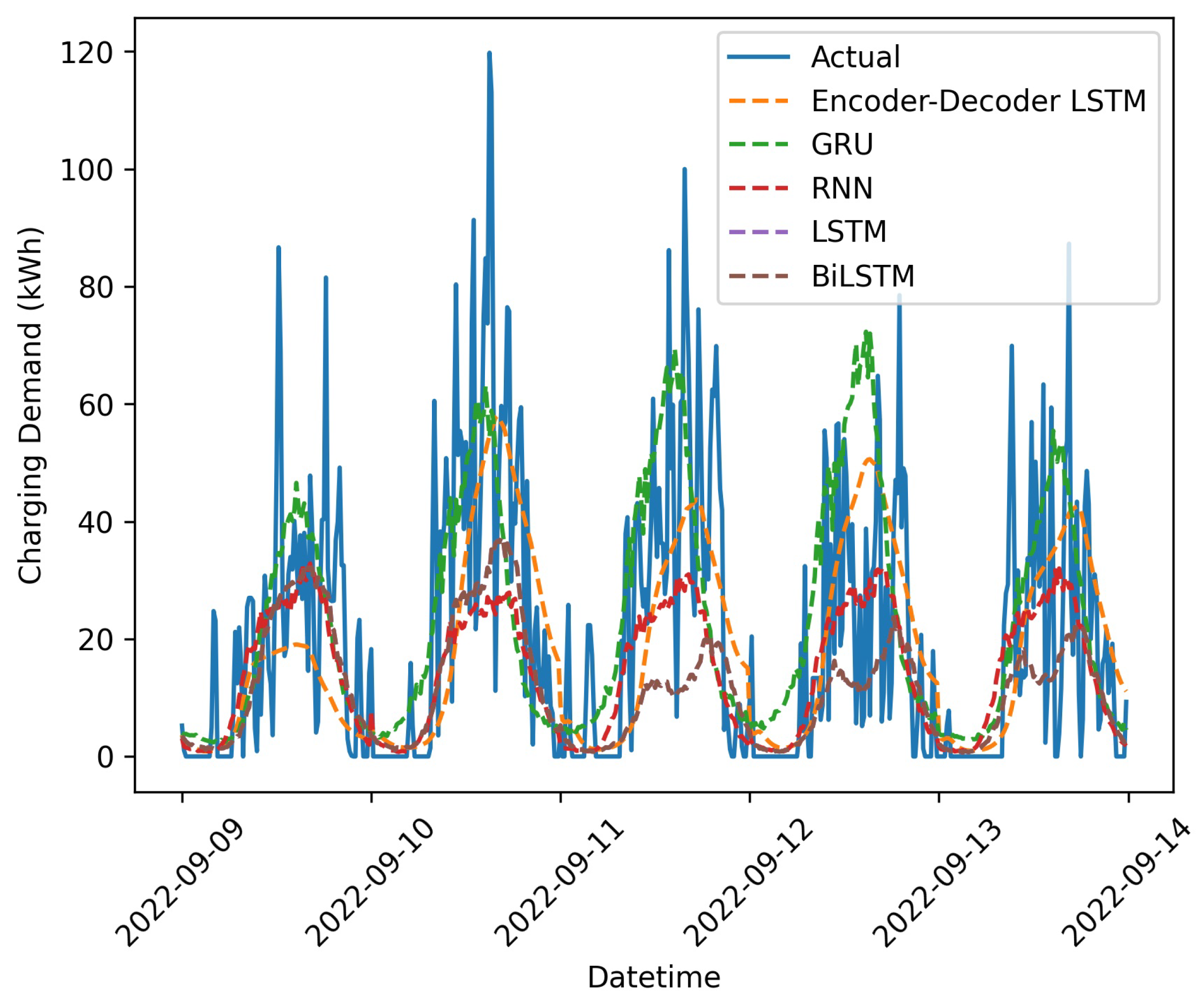
The RNN, LSTM, GRU, and BiLSTM models DL algorithms were implemented for one-step forecasting, while RNN, LSTM, EDLSTM, BiLSTM, and GRU models were used for multistep forecasting. Aggregated data (encompassing all locations) and each location apart were separately analyzed for one-step forecasting. In order to assess the performance of the model, the part of the data that denoted the test set was held out. The rest of the data served as the training set, with 20% of it being used as a validation set to test various hyperparameter configurations with a trial-and-error method [20]. The configuration with the highest performance was selected as the final set of parameters. The configuration of the adopted models is indicated in

Table 7. Model parameters for load demand forecasting.

Forecasting	Level	Model	Epoch	Configuration
Real-time	All locations	RNN	35	Unit 30, dropout 0.0
		LSTM	47	Unit 20, 20; dropout 0.2
		GRU	35
		BiLSTM	30
	Highway	RNN	43	Unit 20, dropout 0.0
		LSTM	53	Unit 20, 20; dropout 0.2
		GRU	32
		BiLSTM	41
	Countryside	RNN	57	Unit 20, dropout 0.0
		LSTM	48	Unit 20, 20; dropout 0.2
		GRU	41
		BiLSTM	46
	Inner city	RNN	66	Unit 20, dropout 0.0
		LSTM	55	Unit 20, 20; dropout 0.2
		GRU	38
		BiLSTM	51
	Near the highway	RNN	63	Unit 20, dropout 0.0
		LSTM	50	Unit 20, 20; dropout 0.2
		GRU	35
		BiLSTM	36
	Outside the city	RNN	60	Unit 20, dropout 0.0
		LSTM	37	Unit 20, 20; dropout 0.2
		GRU	50
		BiLSTM	45
Day-ahead	All locations	RNN	40	Unit 40, dropout 0.0
		LSTM	30	Unit 40, 40; dropout 0.2
		GRU	30
		BiLSTM	35
		EDLSTM	30	Unit 40, 40; dense 10; dropout 0.2

. These models were trained on the entire training set before being evaluated on the holdout test set. The batch size was set to 192, and the learning rate was defined as 0.001 for all models. Dropout is a neural network regularization technique where units are randomly deactivated during training to prevent overfitting and improve generalization [50]. Dropout regularization and early stopping strategies were employed to prevent overfitting during training, with a fixed number of epochs set to 100. Initially, the model was trained for 100 epochs, but signs of overfitting were noticed. To address this, dropout regularization and early stopping techniques were incorporated. Dropouts helped prevent the model from relying too much on specific parts during training. Simultaneously, the early stopping technique, combined with dropouts, intervened when the model’s performance on a separate validation dataset started to decline while training continued to improve, indicating potential overfitting.

4.4. Results

The results of the real-time forecasting are presented in

Table 8. Performance of real-time forecasting based on holdout test data.

Level	Models	MSE (%)	MAE (%)	RMSE (%)
All locations	RNN	0.99	7.03	9.95
	LSTM	0.95	6.72	9.79
	GRU	0.95	6.70	9.70
	BiLSTM	1.03	6.77	10.17
Highway	RNN	0.77	5.29	8.81
	LSTM	0.77	5.17	8.78
	GRU	0.76	5.15	8.75
	BiLSTM	0.78	5.17	9.81
Near the highway	RNN	0.66	3.59	8.15
	LSTM	0.65	3.40	8.07
	GRU	0.61	3.47	7.83
	BiLSTM	0.64	3.71	8.04
Inner city	RNN	0.51	4.44	7.20
	LSTM	0.55	4.28	7.42
	GRU	0.51	4.40	7.18
	BiLSTM	0.55	4.41	7.48
Countryside	RNN	0.54	4.06	7.35
	LSTM	0.51	3.75	7.18
	GRU	0.51	3.89	7.19
	BiLSTM	0.51	4.00	7.20
Outside the city	RNN	0.67	3.15	8.19
	LSTM	0.66	3.19	8.15
	GRU	0.63	3.03	7.97
	BiLSTM	0.64	3.33	8.02

and entail a couple of interesting findings.

• LSTM and GRU had the lowest RMSE for all locations. It is worth noticing that the GRU-based model did better with fewer epochs than the LSTM model most of the time, indicating that it was more efficient because it required less memory and fewer training parameters.
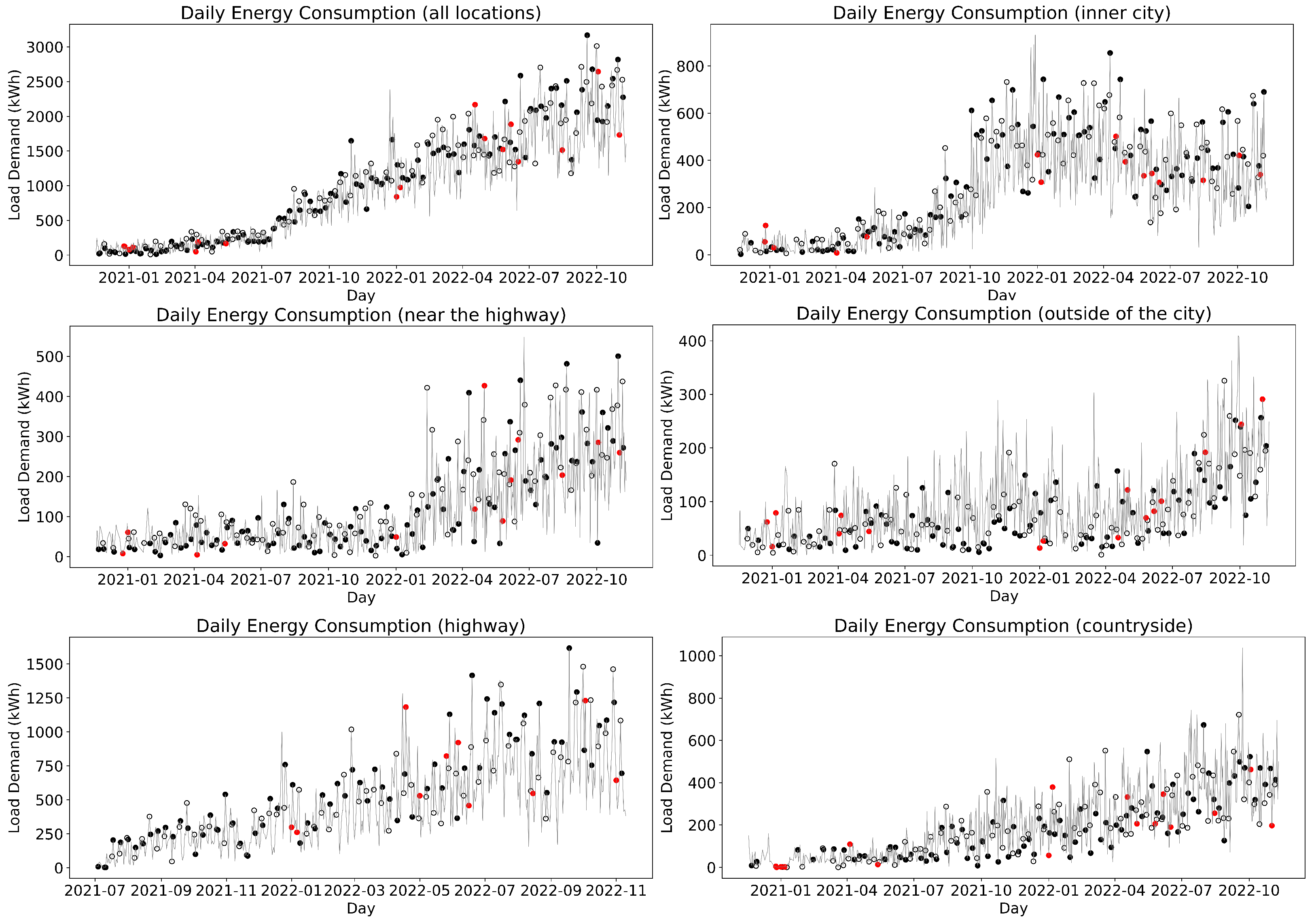
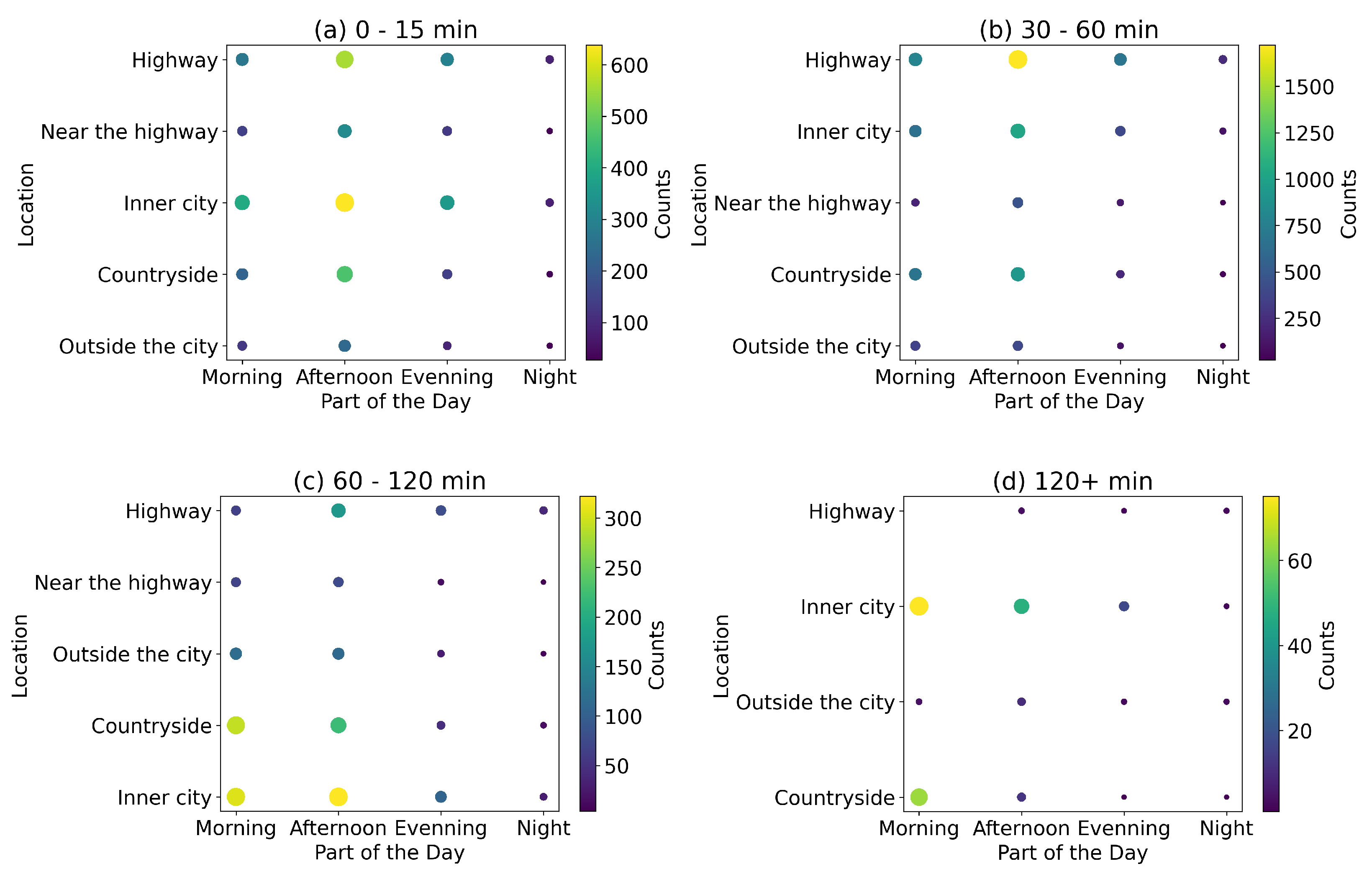
• Forecasts using individual data were more accurate than those based on aggregated data. The accuracy of individual data varied by location. Locations such as the inner city and the countryside achieved better results than other places. This may be due to the charging duration. As illustrated in Figure 10, drivers in the inner city and in the countryside tend to charge their EVs for a longer time, creating a steady two-hour (eight steps) charging pattern. This stability simplifies the prediction for the next steps.

The highway had the worst accuracy among the other locations. This can be explained by the following three effects:

• The highway demonstrated the highest number of EV charging sessions, as depicted in Figure 8, even though the data for the highway were collected over a shorter period of time compared to the other locations, as shown in Figure 9.
• The fluctuations of the highway daily demand ranged from 0 to 1400 kWh (see Figure 9), which made it more challenging to accurately predict the demand compared to other locations, where the variability was much less.
• Charging sessions might show more variability due to the low frequency of long-term charging on the highway, as indicated in Figure 10. This high number of charging sessions could be due to higher traffic volumes or more transient populations. The proposed model provided more accurate forecasting results for each location apart and a longer charging duration.

To visually assess the forecasting result, Figure 11 displays the actual (original) and forecasted demand for a day across six locations: all locations, highway, countryside, inner city, near the highway, and outside the city. The day was randomly chosen from a test dataset that had not been exposed to the models during the training phase. It is clear that the observations and the predicted demands match.

For the day-ahead forecasting, 96 steps of 15 min intervals were predicted.

Table 9. Performance of day-ahead forecasting based on holdout test data.

Level	Models	MSE (%)	MAE (%)	RMSE (%)
All locations	RNN	2.06	9.65	14.38
	LSTM	2.17	9.99	14.73
	GRU	1.90	9.68	13.91
	BiLSTM	2.00	9.81	14.14
	Encoder–decoder LSTM	2.04	9.95	14.29

presents the findings for the day-ahead forecasting using the holdout test set. EDLSTM, GRU, and BiLSTM outperformed the other models with a lower RMSE. However, the BiLSTM required a longer training time than other high-performing models such as the GRU and encoder-decoder LSTM. It can be attributed to BiLSTM’s more complex structure, which consists of two LSTM networks.

Furthermore, Figure 12 illustrates the forecasted results from 9 September 2022 to 14 September 2022. This time frame was selected to cover the period of real-time demand forecasting. The plot reveals that all models exhibited a more accurate forecasting pattern for lower-energy demand. However, when it came to high-demand power, the encoder–decoder LSTM and GRU models outperformed the other models in terms of performance.

5. HESS Scheduling Optimization

5.1. Principle of the HESS Scheduling Algorithm

The overall goal of the scheduling approach was to determine the best time to charge the HESS while prioritizing the use of PV power and minimizing the amount of energy consumed by the grid. It was developed for a 24 h scheduling period with a resolution of 15 min. Figure 13 illustrates the flowchart of the proposed approach. It is composed of two main phases: the “HESS Scheduling”, or the offline phase, and the “Energy Balancing”, or the online phase.

The inputs of the first phase are the day-ahead prediction of PV power data, load demand data, and grid price data. The principle of the HESS scheduling is depicted in Algorithm 1. It runs through the forecasted day to identify the time slots of high-PV production and low-cost grid energy. As a result, it calculates the optimal charging amount of grid energy for these predetermined time slots.

In the second phase, the predicted time slots and charging amounts are combined with real data, i.e., PV power, load demand, and grid prices to balance the energy flow of the day in order to ensure optimal energy management. The principle of “Energy Balancing” is given in Algorithm 2.

Algorithm 1 Scheduling algorithm

1: Input: Grid price, forecasted PV power and forecasted load demand data Constraints information for grid and HESS 2: Output: Optimal charging time Amount of grid energy to charge the HESS 3: begin 4: Define S as set of times when PV exceeds demand 5: Define G as set of cheapest time 6: Define P as set of purchase amount on cheapest time 7: while i to end of the day do Find first time when PV energy exceeds demand 8:     if PV exceeds demand then 9:           Add time to S 10:         Calculate the required energy from i to the time in S. 11:         To calculate the required energy, for each time step, subtract PV power from demand, then sum up all the calculated energy 12:         Sum all of them to find total required energy till the time. 13:         if SoC in time i is greater equal than required energy then 14:            Call energy balance function 15:            Update the system status 16:         else 17:            while SoC in time i is less than required energy do 18:                Find the cheapest time between i and the time in S 19:                Add the cheapest time to set of G 20:                Calculate the required energy (load demand − PV power) from i to cheapest time 21:                Call energy balance function considering the purchases 22:                Update the system status 23:            end while 24:         end if 25:     else 26:         Calculate required energy till for the remaining day 27:         if SoC in time i is greater equal than required energy then 28:            Call energy balance function 29:            Update the system status 30:         else 31:            while SoC in time i is less than required energy do 32:                Find next cheapest time 33:                Add time to set of G 34:                Call energy balance function considering the purchases 35:                Update the system status 36:            end while 37:         end if 38:     end if 39: end while 40: end

Algorithm 2 Energy balancing algorithm

1: Input: Initial SoC, grid price, demand, PV energy, purchases’ times and amounts Constraints information for grid and HESS 2: Output: System status per 15 min interval 3: begin 4: for Every time step do 5:     Define temp_soc = soc 6:     Grid energy = 0 7:     if time step matches with purchase time then 8:         Update grid energy with purchase considering battery limit 9:         Update temp_soc 10:         if PV energy >= demand then 11:            Update temp_soc considering battery limit 12:         else if temp_soc >= demand - PV then 13:            Update temp_soc considering battery limit 14:         else 15:            Update grid considering battery limit 16:            temp_soc = 0 17:         end if 18:     end if 19:     Update soc = temp_soc 20:     Store remaining and initial SoC, demand, PV energy, grid energy, and price with time in system status 21: end for 22: return System status, initial SoC 23: end

The proposed algorithm thoroughly achieved the following key features:

• Energy efficiency: PV power was the main used energy source to meet the demand, and excess PV energy was stored in the HESS.
• Optimization of battery charge/discharge profile: Unlike fully charging or deeply discharging the battery [65], our approach charged the battery with only the required amount of energy needed to maximize solar energy utilization and reduce costs, based on the generated PV power, low energy cost, and battery constraints [65]. This approach inherently contributes to the battery’s overall lifespan by avoiding extreme stress [66]. Furthermore, maintaining a certain discharge limit in the battery can provide a buffer for potential urgent situations where higher energy is unexpectedly needed.
• Cost minimization: Cost minimization was applied first by prioritizing PV power consumption and second by using the grid during the cheapest electricity price time through the following steps of the “Scheduling Algorithm”:
  • Prioritizing PV power consumption: When PV energy generation exceeds demand (Lines 4–23), denoted as set S, it calculates the total required energy to meet the demand from the current time until the time in set S (Lines 10–12). If the HESS’s state of charge (SoC) at the current time is sufficient to meet the required energy, the algorithm balances the energy utilization and updates the system status (Lines 13–15). If the SoC is insufficient, the algorithm finds the cheapest time (set G) between the current time and the time in S. It calculates another required energy between the current time and the cheapest time in G. Then, the second required energy amount is subtracted from the first required energy amount to find the amount to be purchased from the grid at the cheapest time in G (Lines 17–23).
  • Optimizing grid usage when PV generation is below demand: In scenarios where PV generation does not exceed demand until the end of the day (Lines 25–37), the algorithm calculates the total required energy for the remaining day (Line 26). If the SoC at the current time can fulfill this required energy, the energy balance is achieved (Lines 27–29). If not, the algorithm identifies the next cheapest times for energy purchases (Lines 31–36).
• Real-time data: The system was developed and tested using real-time datasets to represent a realistic scenario.
• Single algorithm: The system employed a single algorithm for scheduling throughout the day instead of separate algorithms for daytime and nighttime [67]. This provided a more practical approach, considering seasonal changes in daylight hours.

5.2. Simulation Setup

The grid data used in this paper originated from the real-world context of Germany’s electricity market, obtained from the ENTSO-E Transparency Platform [68]. This dataset includes actual grid prices, denoted in units of EUR/MWh, and provides prices for every 15 min throughout every day. While calculating the cost, the grid price unit was converted from EUR/MWh to EUR/kWh.

The system configuration was as follows:

• The total battery capacity was 620 kWh.
• The battery charge and discharge limit was 20 percent of the total capacity.
• The maximum grid energy for each time slot was 200 kWh.
• The initial battery state of charge (SoC) was 124 kWh, which was a discharge limit.

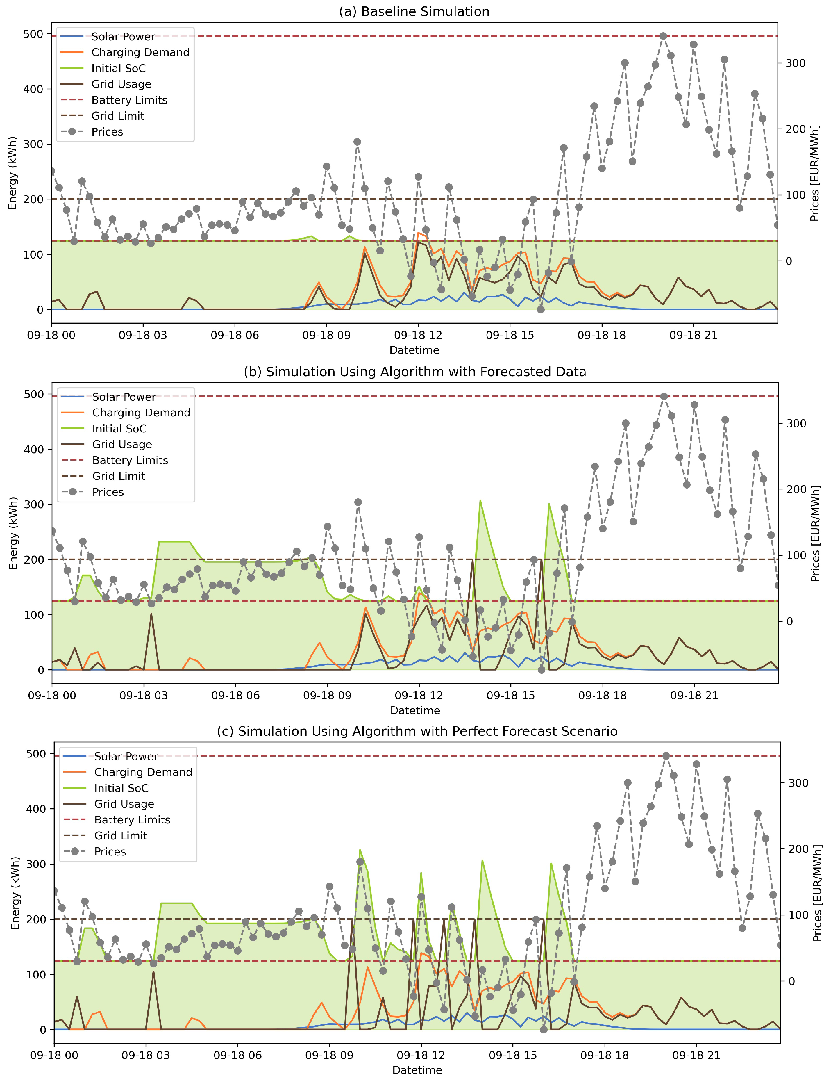
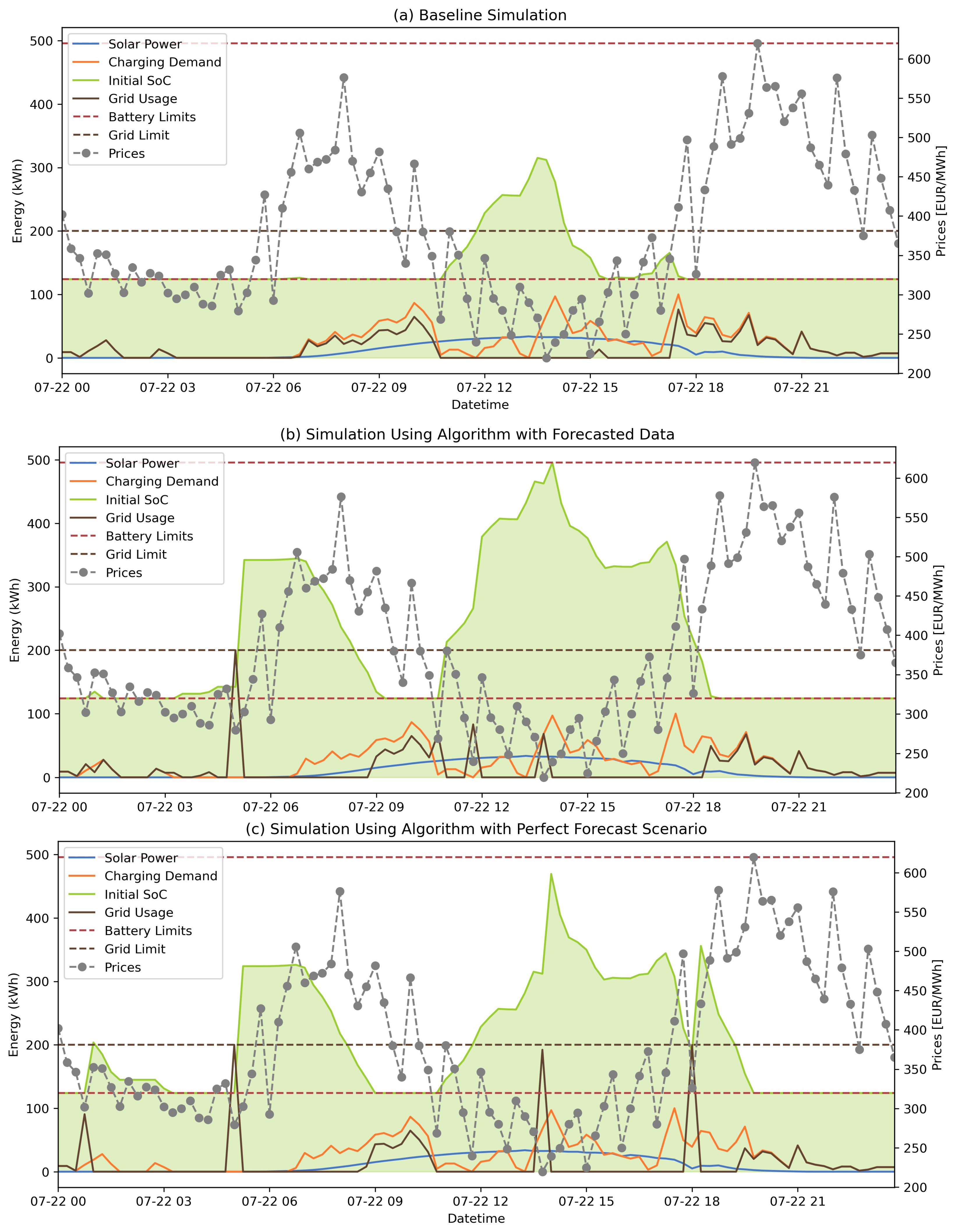
5.3. Simulation Results

To assess the performance of our proposal, three different simulations were launched:

• Baseline simulation or energy balancing simulation: in this case, the simulation ran without predicted data.
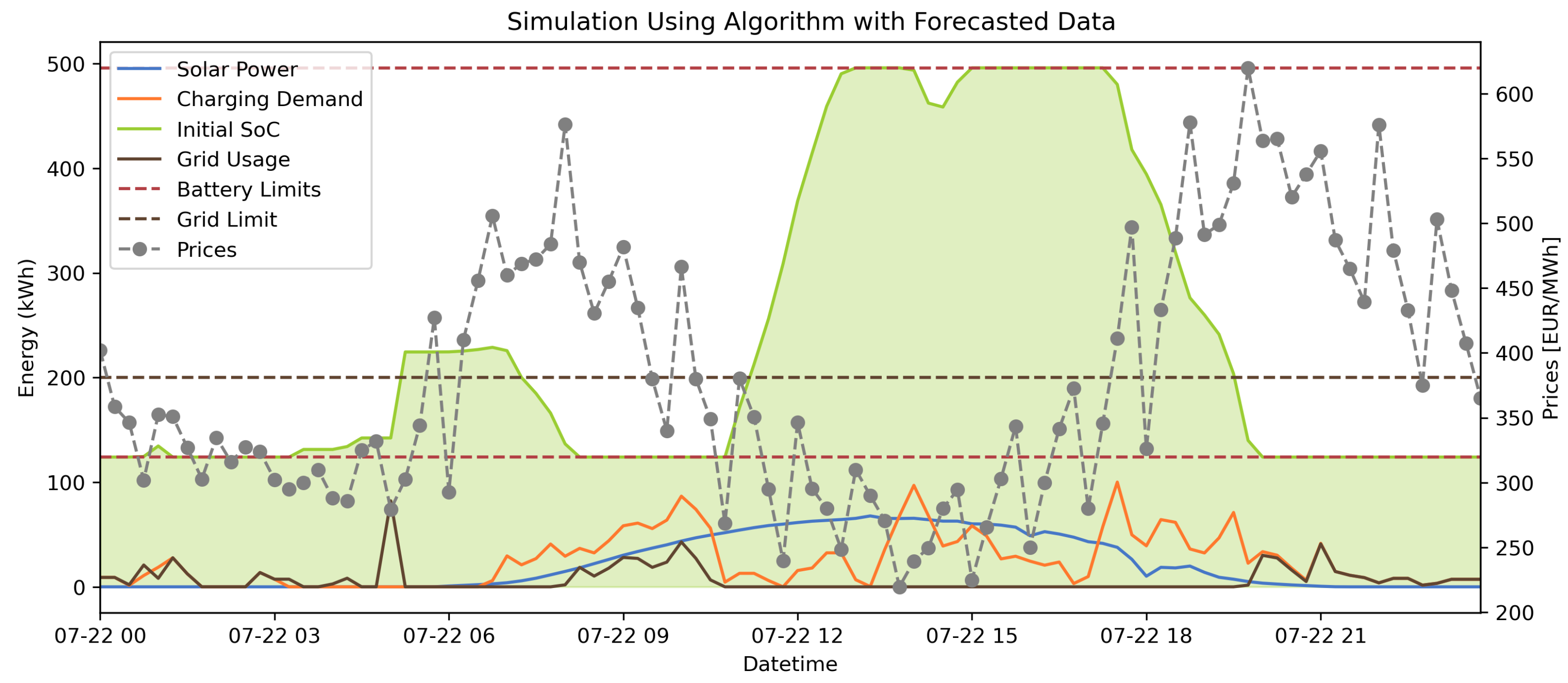
• Simulation with forecasted data: this case corresponded to our proposal.
• Simulation with perfect forecasted data: instead of using predicted data as inputs for the scheduling algorithm, real data were adopted.

Our goal was to have results as close as possible to the “Simulation with perfect forecasted data” as it represented the ideal solution.

Several scenarios were implemented.

5.3.1. Scenario 1: High-Load Demand

For the high-demand scenario, we selected the date of 18 September 2022. We ran the three simulations. The findings, highlighted in Figure 14, demonstrated two things. First, our proposal (Figure 14b) reduced the consumption of grid energy. Second, the graphs of the “Simulation with forecasted data” followed the same pattern as the “Simulation with perfect forecasted data”. We also observed that the grid usage spiked when the grid energy prices were too low.

We calculated in

Table 10. Scenario 1: total grid energy cost.

Simulation	Total Cost	Number of Grid Uses
Baseline	228.42	63
Algorithm with forecasted data	177.21	56
Algorithm with perfect forecast	134.10	47

the total grid energy cost and the number of grid uses. Our proposal reduced the costs by 22.4% and the grid dependability by 11% compared to the “Baseline simulation”.

Table 11. Scenario 1: the optimal time and the amount of grid energy (in kWh) to charge the HESS.

Simulation:	Algorithm with Forecasted Data
Time	00:00	00:15	00:30	00:45	02:45	3:15	10:45	11:45	12:45	13:45	16:00
Amount	8.35	6.96	7.64	39.16	6.17	101.88	35.04	67.14	82.07	200	200
Simulation:	Algorithm with Perfect Forecast
Time	00:00	00:15	00:45	3:15	09:45	10:45	11:45	12:45	13:45	16:00
Amount	13.86	17.82	59.80	105.05	200	58.26	200	200	200	200

presents the optimal charging time for the HESS from the grid and the amount of grid energy to be consumed. From these results, it is clear that our approach is directly in line with the ideal simulation.

5.3.2. Scenario 2: High-PV-Power Production

For this scenario, we selected the day of 22 July 2022. The simulation was conducted separately for three configurations, and the results are displayed in Figure 15.

Table 12. Scenario 2: the optimal time and the amount of energy (kWh) to charge the HESS.

Simulation:	Algorithm with Forecasted Data
Time	00:00	00:15	00:30	00:45	03:15	04:00	04:15	05:00	10:45	11:45	13:45
Amount	1.85	1.75	1.99	20.84	7.30	2.75	8.21	200	67.66	83.04	200
Simulation:	Algorithm with Perfect Forecast
Time	00:00	00:15	00:30	00:45	05:00	13:45	18:00
Amount	9	9	1.44	90	200	192	200

presents the defined optimal charging times for the HESS using the grid for both cases: the forecasted data and the perfect forecast data. The findings in

Table 13. Scenario 2: high PV power—configuration comparison.

Simulation	Total Cost	Number of Grid Uses
Baseline	582.58	52
Algorithm with forecasted data	502.40	45
Algorithm with perfect forecast	468.82	33

demonstrate that the proposed algorithm achieved a significant 12.76% reduction in grid energy cost compared to the baseline simulation. Furthermore, the proposed system successfully reduced grid dependence by 13.46%.

5.3.3. Scenario 3: Intensified High PV Power

In addition to the original high PV power (scenario 2), a further analysis was conducted to examine the algorithm’s performance under even more extreme solar conditions. For this purpose, the PV power data were multiplied by two, representing an intensified PV power. The “simulation using an algorithm with forecasted data” was repeated using these multiplied PV power data. This further analysis allowed for a more comprehensive understanding of the algorithm’s adaptability to varying PV power conditions and provided insights into its PV power usage efficiency.

As depicted in Figure 16, the algorithm exhibited a notable behavior during that simulation. Specifically, it refrained from purchasing energy from the grid during periods of excess solar energy. In contrast, in the high-PV-power scenario (Scenario 2), the algorithm did not prefer grid energy purchases at 14:15. Additionally, as seen in

Table 14. Scenario 3: the optimal time and the amount of energy (kWh) to charge the HESS.

Simulation:	Algorithm with Forecasted Data
Time	00:00	00:15	00:30	00:45	03:15	04:00	04:15	05:00	10:45	11:45
Amount	1.75	1.72	1.98	20.84	7.30	2.75	8.21	82.20	0	0

, in this extreme solar condition (Scenario 3), the algorithm purchased 82.20 kWh of energy from the grid when the grid electricity was cheap at 5:00. This is in contrast to Scenario 2, where it purchased 200 kWh of grid energy at 5:00. The reason for this behavior is that the algorithm anticipated excess PV energy during the day and consequently, it seemed unnecessary to buy 200 kWh from the grid. Instead, it only charged the battery with the energy required to meet the demand until the excess PV energy became available.

This comparison demonstrates the algorithm’s ability to prioritize and maximize the utilization of PV energy over grid energy when excess PV energy is available. The algorithm’s intelligent prioritization strategy significantly improves the use of PV power and minimizes the reliance on grid energy.

Furthermore, we quantified the algorithm’s energy efficiency using the widely recognized self-consumption rate (SCR) metric. The SCR measures how efficiently PV energy is used, considering the fraction used for meeting load demand needs and charging an HESS in relation to the total PV energy generated [69]. The SCR is calculated using the Equation (4).

$$\mathrm{SCR}=\frac{E_{p,d}+E_{p,b}}{E_{p,v}}$$

(4)

where $E_{p,d}$ represents the direct use of PV generation to meet the load demand in kilowatt-hours (kWh). $E_{p,b}$ denotes the PV production utilized for charging the HESS in kWh, and  $E_{p,v}$ represents the total PV generation in kWh [69].

We compared the efficiency of the charging schedule from Scenario 2 with Scenario 3, keeping the input conditions constant at double the solar power, typical demand, and electricity costs. The SCR for Scenario 2 was 74.33%, while for Scenario 3, it was 80.36%. This analysis allowed us to assess the effectiveness of the enhanced charging schedule in Scenario 3 for maximizing solar energy utilization compared to the original scheduling in Scenario 2.

5.3.4. Scenario 4: Monthly Analysis

For the monthly analysis, each day was simulated separately, and the total cost as well as the grid consumption were calculated monthly. As shown in

Table 15. Scenario 3: month analysis.

	Total Cost	Number of Grid Uses
June (21.06.2022–30.06.2022)
Baseline	2484.26	400
Algorithm with forecasted data	2165.53	303
Algorithm with perfect forecast	1992.09	190
July
Baseline	12,263.50	1669
Algorithm with forecasted data	10,877.06	1395
Algorithm with perfect forecast	10,124.34	946
August
Baseline	16,083.30	1641
Algorithm with forecasted data	14,452.38	1243
Algorithm with perfect forecast	14,093.80	977
September
Baseline	14,930.79	1581
Algorithm with forecasted data	13,037.64	1308
Algorithm with perfect forecast	12,556.51	1009
October
Baseline	8381.63	1845
Algorithm with forecasted data	7029.69	1435
Algorithm with perfect forecast	6866.35	1236
November (01.11.2022–10.11.2022)
Baseline	1867.26	542
Algorithm with forecasted data	1650.11	466
Algorithm with perfect forecast	1637.46	413

, our proposed model consistently reduced the grid energy cost compared to the baseline model, with an average equal to 12.13% every month. The highest cost reduction was observed in October, with a reduction of 16%. This could be attributed to the relatively higher grid prices in October compared to other months. Conversely, the lowest cost reduction occurred in August, at a rate of 10.12%.

Our proposed charging scheduling algorithm was evaluated under three distinct scenarios. The time slots 00:00, 00:15, and 00:30 were identified as crucial for charging the HESS from the grid across the three scenarios. The most important improvement was observed in the first scenario (i.e., the high-load demand), demonstrating a cost reduction of 22.4% and a decrease in grid dependency by 11%. This reduction in cost during high-demand periods could be attributed to the system’s reliance on the grid. Therefore, minimizing the use of expensive grid power had a more positive impact on overall costs.

There are several reasons that impact the cost reduction; one of the important factors that influences the cost reductions achieved through our energy management system is the limit on the power that can be purchased from the grid. Our system was constrained to a maximum of 200 kWh from the grid. This limit has a direct influence on the cost savings we can realize. When the demand for power is high or renewable generation is low, our system has to rely more heavily on grid power. Once the 200 kWh limit is reached, the system might need to resort to more expensive or less efficient options, leading to smaller cost reductions. Conversely, on days with low power demand or high renewable generation, the system can operate well within the grid power limit, leading to larger cost reductions. Another important factor is the energy storage capacity of our system, represented by the battery limit that influences the cost minimization process. The battery’s capacity determines the amount of power that can be stored during periods of excess generation or low demand, which can then be used during high-demand periods or when generation is low. Hence, the larger the battery capacity, the greater the potential for cost savings, as more power can be stored and used later, reducing reliance on more expensive grid power. In the next section, we discuss the main findings of our paper and explore possible directions for future research.

6. Conclusions

This paper presented a comprehensive, multistage approach to determining the optimal time for charging an HESS at EV charging stations. This approach addressed major challenges in energy management systems, including forecasting PV power and charging load demand and ensuring a cost- and resource-efficient use of HESS. To achieve optimal scheduling for the HESS, a three-stage strategy was proposed. In the first stage, we executed univariate PV power forecasting using various DL models for real-time and day-ahead forecasting. The motivation for forecasting PV power was to obtain day-ahead PV power data for the subsequent day in order to identify times of PV power excess. This enabled us to prepare an HESS that considered these times and more efficiently used PV power. For 15 min ahead forecasts, LSTM and GRU models demonstrated superior performance in terms of RMSE with 5.78% and 5.79%, respectively. For day-ahead forecasting, the encoder–decoder LSTM network performed better, with an RMSE of 11.71%. The forecasting results aligned with industry standards for real-time and day-ahead scenarios. Accordingly, the error was generally around 5–7% for one-to-two-hour forecasting [56,57,58] and should not exceed a 20% RMSE for forecasting one to many hours [70,71].

In the second stage, multivariate load demand forecasting was applied using the same models as in stage one for real-time and day-ahead forecasting for aggregated locations and each location apart. The reason to implement this stage was to predict the upcoming load demand and define the optimal HESS charging time to meet the demand. Moreover, we analyzed the effect of location characteristics on forecasting. The result demonstrated that the proposed algorithm performed better in every location with longer charging times and fewer charging sessions, such as the inner city and countryside. The worst result was on highways. Moreover, in aggregated locations, the GRU model reached a 9.70% RMSE score for real-time forecasting, and a 13.91% RMSE for day-ahead forecasting.

In the final stage, a scheduling algorithm was developed to account for energy changes in load demand and PV power throughout the day. In order to anticipate these changes in advance, the most accurate forecasting results from the first two stages were utilized in the optimal energy management algorithm. This allowed the system to determine the best times for charging while maximizing PV power utilization and minimizing grid energy costs. Experimental results of the proposed system demonstrated an average cost reduction of 12.13%, providing an efficient and cost-effective solution for energy management systems in charging stations. Moreover, the system reduced grid dependency by 19.9% compared to systems that did not employ predictive scheduling.

Although this study has significantly contributed to the field, there are several promising directions for future research. These future considerations are particularly relevant for each segment of this paper, encompassing solar forecasting, demand forecasting, and optimal HESS scheduling. In demand forecasting, it would be beneficial to consider additional features such as weather and temperature that could indirectly influence driver behavior and affect the charging pattern. Further analysis can be performed using different versions of the models implemented in this work, such as those incorporating attention mechanisms or ensemble models that combine the strengths of multiple individual models. Furthermore, experimenting with different lengths of the forecast horizon, extending from two days to one week, might yield valuable findings.

References

1. Omondi, B. The Most Polluting Industries in 2022. 2022. Available online: https://ecojungle.net/post/the-most-polluting-industries-in-2021/ (accessed on 4 June 2023).
2. Omondi, B. Greenhouse Gas Emissions from Transport in Europe. 2022. Available online: https://www.eea.europa.eu/ims/greenhouse-gas-emissions-from-transport (accessed on 4 June 2023).
3. Kabir, M.E.; Assi, C.; Tushar, M.H.K.; Yan, J. Optimal scheduling of EV charging at a solar power-based charging station. IEEE Syst. J. 2020, 14, 4221–4231. [Google Scholar] [CrossRef]
4. Cazzola, P.; Gorner, M.; Schuitmaker, R.; Maroney, E. Global EV Outlook 2016; International Energy Agency: Paris, France, 2016. [Google Scholar]
5. Commission, European Causes of Climate Change. Available online: https://climate.ec.europa.eu/climate-change/causes-climate-change_en (accessed on 8 June 2023).
6. Limouniac, T.; Yaagoubib, R.; Bouzianec, K.; Guissia, K.; Baalia, E.H. Univariate and multivariate LSTM models for one step and multistep PV power forecasting. Int. J. Renew. Energy Dev. 2022, 11, 815. [Google Scholar] [CrossRef]
7. Yang, T.; Li, X.; Qi, L.; Hui, D.; Jia, X. A schedule method of battery energy storage system (BESS) to track day-ahead photovoltaic output power schedule based on short-term photovoltaic power prediction. In Proceedings of the International Conference on Renewable Power Generation (RPG 2015), Beijing, China, 17–18 October 2015. [Google Scholar]
8. Suresh, V.; Janik, P.; Rezmer, J.; Leonowicz, Z. Forecasting solar PV output using convolutional neural networks with a sliding window algorithm. Energies 2020, 13, 723. [Google Scholar] [CrossRef]
9. Chaudhary, G.; Lamb, J.J.; Burheim, O.S.; Austbø, B. Review of energy storage and energy management system control strategies in microgrids. Energies 2021, 14, 4929. [Google Scholar] [CrossRef]
10. Atawi, I.E.; Al-Shetwi, A.Q.; Magableh, A.M.; Albalawi, O.H. Recent Advances in Hybrid Energy Storage System Integrated Renewable Power Generation: Configuration, Control, Applications, and Future Directions. Batteries 2022, 9, 29. [Google Scholar] [CrossRef]
11. Sharma, E. Energy forecasting based on predictive data mining techniques in smart energy grids. Energy Inform. 2018, 1, 367–373. [Google Scholar] [CrossRef]
12. Shirinda, K.; Kanzumba, K. A review of hybrid energy storage systems in renewable energy applications. Int. J. Smart Grid Clean Energy 2022, 11, 99–108. [Google Scholar] [CrossRef]
13. Schubert, C.; Hassen, W.F.; Poisl, B.; Seitz, S.; Schubert, J.; Usabiaga, E.O.; Gaudo, P.M.; Pettinger, K.H. Hybrid Energy Storage Systems Based on Redox-Flow Batteries: Recent Developments, Challenges, and Future Perspectives. Batteries 2023, 9, 211. [Google Scholar] [CrossRef]
14. Titus, F.; Thanikanti, S.B.; Deb, S.; Kumar, N.M. Charge scheduling optimization of plug-in electric vehicle in a PV powered grid-connected charging station based on day-ahead solar energy forecasting in Australia. Sustainability 2022, 14, 3498. [Google Scholar]
15. Corchero, C.; Cruz-Zambrano, M.; Heredia, F.J. Optimal energy management for a residential microgrid including a vehicle-to-grid system. IEEE Trans. Smart Grid 2014, 5, 2163–2172. [Google Scholar]
16. Wu, H.; Li, H.; Gu, X. Optimal energy management for microgrids considering uncertainties in renewable energy generation and load demand. Processes 2020, 8, 1086. [Google Scholar] [CrossRef]
17. Lee, S.J.; Yoon, Y. Electricity cost optimization in energy storage systems by combining a genetic algorithm with dynamic programming. Mathematics 2020, 8, 1526. [Google Scholar] [CrossRef]
18. Hossain, M.A.; Pota, H.R.; Squartini, S.; Abdou, A.F. Modified PSO algorithm for real-time energy management in grid-connected microgrids. Renew. Energy 2019, 136, 746–757. [Google Scholar] [CrossRef]
19. Konstantinou, M.; Peratikou, S.; Charalambides, A.G. Solar photovoltaic forecasting of power output using lstm networks. Atmosphere 2021, 12, 124. [Google Scholar] [CrossRef]
20. Van Kriekinge, G.; De Cauwer, C.; Sapountzoglou, N.; Coosemans, T.; Messagie, M. Day-ahead forecast of electric vehicle charging demand with deep neural networks. World Electr. Veh. J. 2021, 12, 178. [Google Scholar] [CrossRef]
21. Cadete, E.; Ding, C.; Xie, M.; Ahmed, S.; Jin, Y.F. Prediction of electric vehicles charging load using long short-term memory model. In Tran-SET 2021; American Society of Civil Engineers: Reston, VA, USA, 2021; pp. 52–58. [Google Scholar]
22. Boulakhbar, M.; Farag, M.; Benabdelaziz, K.; Kousksou, T.; Zazi, M. A deep learning approach for prediction of electrical vehicle charging stations power demand in regulated electricity markets: The case of Morocco. Clean. Energy Syst. 2022, 3, 100039. [Google Scholar] [CrossRef]
23. Cespedes, A.J.J.; Pangestu, B.H.B.; Hanazawa, A.; Cho, M. Performance Evaluation of Machine Learning Methods for Anomaly Detection in CubeSat Solar Panels. Appl. Sci. 2022, 12, 8634. [Google Scholar] [CrossRef]
24. Lim, S.C.; Huh, J.H.; Hong, S.H.; Park, C.Y.; Kim, J.C. Solar Power Forecasting Using CNN-LSTM Hybrid Model. Energies 2022, 15, 8233. [Google Scholar] [CrossRef]
25. Das, U.K.; Tey, K.S.; Seyedmahmoudian, M.; Mekhilef, S.; Idris, M.Y.I.; Van Deventer, W.; Horan, B.; Stojcevski, A. Forecasting of photovoltaic power generation and model optimization: A review. Renew. Sustain. Energy Rev. 2018, 81, 912–928. [Google Scholar] [CrossRef]
26. Akhter, M.N.; Mekhilef, S.; Mokhlis, H.; Almohaimeed, Z.M.; Muhammad, M.A.; Khairuddin, A.S.M.; Akram, R.; Hussain, M.M. An hour-ahead PV power forecasting method based on an RNN-LSTM model for three different PV plants. Energies 2022, 15, 2243. [Google Scholar] [CrossRef]
27. Gasparin, A.; Lukovic, S.; Alippi, C. Deep learning for time series forecasting: The electric load case. CAAI Trans. Intell. Technol. 2022, 7, 1–25. [Google Scholar] [CrossRef]
28. Time Series Forecasting. 2022. Available online: https://www.tensorflow.org/tutorials/structured_data/time_series#normalize_the_data (accessed on 15 December 2022).
29. Alfian, G.; Syafrudin, M.; Anshari, M.; Benes, F.; Atmaji, F.T.D.; Fahrurrozi, I.; Hidayatullah, A.F.; Rhee, J. Blood glucose prediction model for type 1 diabetes based on artificial neural network with time-domain features. Biocybern. Biomed. Eng. 2020, 40, 1586–1599. [Google Scholar] [CrossRef]
30. Jacoby, D.; Ostrometzky, J.; Messer, H. Short-term prediction of the attenuation in a commercial microwave link using LSTM-based RNN. In Proceedings of the 2020 28th European Signal Processing Conference (EUSIPCO), Amsterdam, The Netherlands, 18–21 January 2021; pp. 1628–1632. [Google Scholar]
31. Bontempi, G.; Ben Taieb, S.; Le Borgne, Y.A. Machine learning strategies for time series forecasting. In Business Intelligence: Second European Summer School, Proceedings of eBISS 2012, Brussels, Belgium, 15–21 July 2012, Tutorial Lectures 2; Springer: Berlin/Heidelberg, Germany, 2013; pp. 62–77. [Google Scholar]
32. Sharadga, H.; Hajimirza, S.; Balog, R.S. Time series forecasting of solar power generation for large-scale photovoltaic plants. Renew. Energy 2020, 150, 797–807. [Google Scholar] [CrossRef]
33. Rumelhart, D.E.; Hinton, G.E.; Williams, R.J. Learning representations by back-propagating errors. Nature 1986, 323, 533–536. [Google Scholar] [CrossRef]
34. Lipton, Z.C.; Berkowitz, J.; Elkan, C. A critical review of recurrent neural networks for sequence learning. arXiv 2015, arXiv:1506.00019. [Google Scholar]
35. Bengio, Y.; Simard, P.; Frasconi, P. Learning long-term dependencies with gradient descent is difficult. IEEE Trans. Neural Networks 1994, 5, 157–166. [Google Scholar] [CrossRef]
36. Hochreiter, S.; Schmidhuber, J. Long short-term memory. Neural Comput. 1997, 9, 1735–1780. [Google Scholar] [CrossRef]
37. Cho, K.; Van Merriënboer, B.; Bahdanau, D.; Bengio, Y. On the properties of neural machine translation: Encoder-decoder approaches. arXiv 2014, arXiv:1409.1259. [Google Scholar]
38. Chollet, F. Chapter 14 Conclusions. In Deep Learning with Python; Manning: New York, NY, USA, 2021. [Google Scholar]
39. Pi, M.; Jin, N.; Chen, D.; Lou, B. Short-term solar irradiance prediction based on multichannel LSTM neural networks using edge-based IoT system. Wirel. Commun. Mob. Comput. 2022, 2022, 2372748. [Google Scholar] [CrossRef]
40. Cheng, X.; Tang, H.; Wu, Z.; Liang, D.; Xie, Y. BILSTM-Based Deep Neural Network for Rock-Mass Classification Prediction Using Depth-Sequence MWD Data: A Case Study of a Tunnel in Yunnan, China. Appl. Sci. 2023, 13, 6050. [Google Scholar] [CrossRef]
41. Sutskever, I.; Vinyals, O.; Le, Q.V. Sequence to sequence learning with neural networks. arXiv 2014, arXiv:1409.3215. [Google Scholar]
42. Yongsheng, D.; Fengshun, J.; Jie, Z.; Zhikeng, L. A short-term power output forecasting model based on correlation analysis and ELM-LSTM for distributed PV system. J. Electr. Comput. Eng. 2020, 2020, 2051232. [Google Scholar] [CrossRef]
43. Zhang, X.; Liu, Y.; Yang, M.; Zhang, T.; Young, A.A.; Li, X. Comparative study of four time series methods in forecasting typhoid fever incidence in China. PLoS ONE 2013, 8, e63116. [Google Scholar] [CrossRef] [PubMed]
44. Westerveld, J.J.; van den Homberg, M.J.; Nobre, G.G.; van den Berg, D.L.; Teklesadik, A.D.; Stuit, S.M. Forecasting transitions in the state of food security with machine learning using transferable features. Sci. Total Environ. 2021, 786, 147366. [Google Scholar] [CrossRef]
45. Fuadah, Y.N.; Pramudito, M.A.; Lim, K.M. An Optimal Approach for Heart Sound Classification Using Grid Search in Hyperparameter Optimization of Machine Learning. Bioengineering 2022, 10, 45. [Google Scholar] [CrossRef]
46. Panigrahi, A.; Patra, M.R. Network intrusion detection model based on fuzzy-rough classifiers. In Handbook of Neural Computation; Elsevier: Amsterdam, The Netherlands, 2017; pp. 109–125. [Google Scholar]
47. Shojaei, A.; Flood, I. Univariate modeling of the timings and costs of unknown future project streams: A case study. Int. J. Adv. Sys. Meas. 2018, 11, 36–46. [Google Scholar]
48. Kingma, D.P.; Ba, J. Adam: A method for stochastic optimization. arXiv 2014, arXiv:1412.6980. [Google Scholar]
49. Cerqueira, V.; Torgo, L.; Smailović, J.; Mozetič, I. A comparative study of performance estimation methods for time series forecasting. In Proceedings of the 2017 IEEE International Conference on Data Science and Advanced Analytics (DSAA), Tokyo, Japan, 19–21 October 2017; pp. 529–538. [Google Scholar]
50. Srivastava, N.; Hinton, G.; Krizhevsky, A.; Sutskever, I.; Salakhutdinov, R. Dropout: A simple way to prevent neural networks from overfitting. J. Mach. Learn. Res. 2014, 15, 1929–1958. [Google Scholar]
51. Kuo, W.C.; Chen, C.H.; Hua, S.H.; Wang, C.C. Assessment of Different Deep Learning Methods of Power Generation Forecasting for Solar PV System. Appl. Sci. 2022, 12, 7529. [Google Scholar] [CrossRef]
52. Lee, W.; Kim, K.; Park, J.; Kim, J.; Kim, Y. Forecasting solar power using long-short term memory and convolutional neural networks. IEEE Access 2018, 6, 73068–73080. [Google Scholar] [CrossRef]
53. Dairi, A.; Harrou, F.; Sun, Y.; Khadraoui, S. Short-term forecasting of photovoltaic solar power production using variational auto-encoder driven deep learning approach. Appl. Sci. 2020, 10, 8400. [Google Scholar] [CrossRef]
54. Zhang, J.; Verschae, R.; Nobuhara, S.; Lalonde, J.F. Deep photovoltaic nowcasting. Sol. Energy 2018, 176, 267–276. [Google Scholar] [CrossRef]
55. Gensler, A.; Henze, J.; Sick, B.; Raabe, N. Deep Learning for solar power forecasting—An approach using AutoEncoder and LSTM Neural Networks. In Proceedings of the 2016 IEEE International Conference on Systems, Man, and Cybernetics (SMC), Budapest, Hungary, 9–12 October 2016; pp. 2858–2865. [Google Scholar]
56. Gao, M.; Li, J.; Hong, F.; Long, D. Short-term forecasting of power production in a large-scale photovoltaic plant based on LSTM. Appl. Sci. 2019, 9, 3192. [Google Scholar] [CrossRef]
57. Lee, D.; Kim, K. Recurrent neural network-based hourly prediction of photovoltaic power output using meteorological information. Energies 2019, 12, 215. [Google Scholar] [CrossRef]
58. Gao, M.; Li, J.; Hong, F.; Long, D. Day-ahead power forecasting in a large-scale photovoltaic plant based on weather classification using LSTM. Energy 2019, 187, 115838. [Google Scholar] [CrossRef]
59. Harrou, F.; Kadri, F.; Sun, Y. Forecasting of photovoltaic solar power production using LSTM approach. In Advanced Statistical Modeling, Forecasting, and Fault Detection in Renewable Energy Systems; IntechOpen: London, UK, 2020; Volume 3. [Google Scholar] [CrossRef]
60. Bouktif, S.; Fiaz, A.; Ouni, A.; Serhani, M.A. Optimal deep learning lstm model for electric load forecasting using feature selection and genetic algorithm: Comparison with machine learning approaches. Energies 2018, 11, 1636. [Google Scholar] [CrossRef]
61. Peixeiro, M. Time Series Forecasting in Python; Manning Publications: New York, NY, USA, 2022. [Google Scholar]
62. Ziyin, L.; Hartwig, T.; Ueda, M. Neural networks fail to learn periodic functions and how to fix it. Adv. Neural Inf. Process. Syst. 2020, 33, 1583–1594. [Google Scholar]
63. Skomski, E.; Lee, J.Y.; Kim, W.; Chandan, V.; Katipamula, S.; Hutchinson, B. Sequence-to-sequence neural networks for short-term electrical load forecasting in commercial office buildings. Energy Build. 2020, 226, 110350. [Google Scholar] [CrossRef]
64. Bishop, C.M.; Nasrabadi, N.M. Pattern Recognition and Machine Learning; Springer: Berlin/Heidelberg, Germany, 2006; Volume 4. [Google Scholar]
65. Abji, N.; Tizghadam, A.; Leon-Garcia, A. Energy storage management in core networks with renewable energy in time-of-use pricing environments. In Proceedings of the 2015 IEEE International Conference on Communications (ICC), London, UK, 8–12 June 2015; pp. 135–141. [Google Scholar]
66. Abdin, Z.; Khalilpour, K.R. Single and polystorage technologies for renewable-based hybrid energy systems. In Polygeneration with Polystorage for Chemical and Energy Hubs; Elsevier: Amsterdam, The Netherlands, 2019; pp. 77–131. [Google Scholar]
67. Kong, J.; Jufri, F.H.; Kang, B.O.; Jung, J. Development of ESS scheduling algorithm to maximize the potential profitability of PV generation supplier in South Korea. J. Electr. Eng. Technol. 2018, 13, 2227–2235. [Google Scholar]
68. Entsoe. ENTSO-E Transparency BZN|DE-LU. Available online: https://transparency.entsoe.eu/transmission-domain/r2/dayAheadPrices/show?name=&defaultValue=false&viewType=GRAPH&areaType=BZN&atch=false&dateTime.dateTime=06.06.2023+00:00|CET|DAY&biddingZone.values=CTY|10Y1001A1001A83F!BZN|10Y1001A1001A82H&resolution.values=PT15M&resolution.values=PT30M&resolution.values=PT60M&dateTime.timezone=CET_CEST&dateTime.timezone_input=CET+(UTC+1)+/+CEST+(UTC+2) (accessed on 6 May 2023).
69. Zhao, Y.; Qin, X.; Shi, X. A Comprehensive Evaluation Model on Optimal Operational Schedules for Battery Energy Storage System by Maximizing Self-Consumption Strategy and Genetic Algorithm. Sustainability 2022, 14, 8821. [Google Scholar] [CrossRef]
70. Iheanetu, K.J. Solar Photovoltaic Power Forecasting: A Review. Sustainability 2022, 14, 17005. [Google Scholar] [CrossRef]
71. Ratshilengo, M.; Sigauke, C.; Bere, A. Short-Term Solar Power Forecasting Using Genetic Algorithms: An Application Using South African Data. Appl. Sci. 2021, 11, 4214. [Google Scholar] [CrossRef]
Figure 1. Charging station overall architecture.
Energies 16 06656 g001
Figure 2. The proposed approach for optimal HESS charging scheduling comprises two primary blocks: “Time Series Forecasting” and “HESS Scheduling and Energy Balance”. The first block forecasts PV power and load demand; the second block leverages these forecasts to determine the optimal time and amount for charging the HESS using the “HESS scheduling algorithm”. Subsequently, the “Energy balance algorithm” employs this defined time and amount to facilitate real-time, optimal energy management.
Energies 16 06656 g002
Figure 3. PV power generation from 2017 to 2021.
Energies 16 06656 g003
Figure 4. Illustration of the sliding-window approach for single-step and multistep forecasting.
Energies 16 06656 g004
Figure 5. Time series cross-validated grid search [44].
Energies 16 06656 g005
Figure 6. Real-time PV power forecast.
Energies 16 06656 g006
Figure 7. Day-ahead PV power forecast.
Energies 16 06656 g007
Figure 8. Load demand by location. The line plot represents the number of charging sessions.
Energies 16 06656 g008
Figure 9. Load demand profile for the different locations. White and black dots correspond to Saturdays and Sundays, respectively. The red dots illustrate the public holidays in Germany, and the line plot denotes the remaining weekdays.
Energies 16 06656 g009
Figure 10. Charging duration: 0–15 min, 30–60 min, 60–120 min, 120+ min.
Energies 16 06656 g010
Figure 11. Real-time demand forecast.
Energies 16 06656 g011
Figure 12. Day-ahead demand forecast.
Energies 16 06656 g012
Figure 13. Proposed HESS scheduling approach.
Energies 16 06656 g013
Figure 14. Scenario 1: high-load demand simulation results.
Energies 16 06656 g014
Figure 15. Scenario 2: high PV power simulation results.
Energies 16 06656 g015
Figure 16. Scenario 3: intensified high PV power.
Energies 16 06656 g016