Energy-Aware Evolutionary Algorithm for Scheduling Jobs of Charging Electric Vehicles in an Autonomous Charging Station

Abstract

The paper considers an innovative model of autonomous charging stations where a program implementing a scheduling algorithm and a set of jobs being scheduled are driven by the same common power source. It is assumed that one of the well-known local search metaheuristics—an evolutionary algorithm—is used for the scheduling process. The algorithm is designed to search for a sequence of charging jobs resulting in a schedule of the minimum length. Since processors with variable processing speeds can be used for computations, this has interesting consequences both from a theoretical and practical point of view. It is shown in the paper that the problem of choosing the right processor speed under given constraints and an assumed scheduling criterion is a non-trivial one. We formulate a general problem of determining the computation speed of the evolutionary algorithm based on the proposed model of a computational task and the adopted problem of scheduling charging jobs. The novelty of the paper consists of two aspects: (i) proposing the new model of the autonomous charging station operating according to the basics of edge computing; and (ii) developing the methodology for dynamically changing the computational speed, taking into account power and energy constraints as well as the results of computations obtained in the current iteration of the algorithm. Some approaches for selecting the appropriate speed of computations are proposed and discussed. Conclusions and possible directions for future research are also given.

1. Introduction

Edge computing [1,2] is a distributed computing paradigm that brings computation and data storage closer to the machines, devices, and sensors that produce and consume data. The term “edge” refers to the boundary between the network and the physical world where data are generated. It aims to reduce the latency and bandwidth requirements of traditional cloud computing by processing data and running applications on the edge of the network rather than in a centralized data center.

In edge computing, computing resources are deployed at the edge of the network, which can be a mobile device, a router, a gateway, or a server located close to the data source. This allows data to be processed in real-time without the need to transmit it back and forth between the device and a remote data center. Edge computing is especially useful for applications that require low latency, high bandwidth, and high availability, such as video streaming, autonomous vehicles, industrial automation, and Internet of Things (IoT) [3,4] devices.

Edge computing can also provide enhanced security and privacy, as sensitive data can be processed and analyzed locally without the need to transmit it to a remote server or data center. It can also enable offline operation, as devices can continue to function and process data even when disconnected from the network. Overall, edge computing represents a shift away from centralized computing architectures towards distributed, decentralized systems that are more efficient, scalable, and resilient. It also has the potential to reduce the cost and complexity of cloud computing, as it can offload some of the processing and storage tasks from the cloud to the edge devices. However, it also raises new challenges, such as, e.g., the management of distributed resources.

Edge computing is particularly justified when certain devices have difficult, restricted, or even impossible access to worldwide network resources. Under such circumstances, edge computing may become a necessity. If we additionally assume that access to the power source is also restricted, conducting effective computations in such a situation is very much a nontrivial task.

In this paper, we consider a case when an advanced device is isolated from a cloud and, additionally, the available power supply is also limited. Such a situation can occur quite often in the real world. Both limitations—access to network resources and access to a constant power source—are characteristic of various practical, battery-powered hardware solutions used in sparsely urbanized areas.

The novelty of the research presented in the paper concerns a few aspects. Firstly, we present an innovative model of an autonomous energy charging station as an example of the situation discussed above. Such a station allows for the charging of a fleet of some energy-powered equipment like, e.g., wheeled vehicles (Electric Motor Vehicles—EMVs), drones (Unmanned Aerial Vehicles—UAVs), or others. We describe the concept of such an autonomous station, which consists of a computing module and an executive module, both supplied by common energy storage. The executive module is responsible for performing the task of charging the fleet of electric vehicles. A well-known metaheuristic, an evolutionary algorithm (EA), has been adopted as the computation method used by the computing module of the station. Secondly, we formulate the original problem of minimizing the charging task schedule length while meeting the imposed deadline as well as the power and energy constraints imposed on the entire station. Thirdly, the main innovation of the overall approach proposed in the paper is that the speed of the computations (and, consequently, the energy consumed by the computations) is dynamically adjusted to their results, i.e., the solutions obtained in successive iterations. It should be stressed that distributing energy between the process of computation and the charging procedure that is ultimately implemented is a very complex task. Too fast computations can result in energy consumption beyond the limit necessary for the completion of all charging tasks. On the other hand, saving energy by slowing down computations can lead to schedules of charging tasks that are very far from the optimum. It is therefore necessary to find a balance between the need to save energy consumed by computations and conducting an energy-intensive search for better schedules. Lastly, we also propose a few approaches to find solutions to the formulated problem; in particular, we discuss a safe approach, an aggressive approach, and an aggressive approach with stopping. We discuss each of them extensively as well as give some indications concerning their possible applications in practice.

The paper then addresses scheduling issues in the context of edge computing and IoT, which, obviously, have been considered in several papers before. An extensive survey on resource scheduling in edge computing is given in [5]. A deep learning-based framework providing a solution and unification of deep learning techniques,, allowing hybrid parallelization and operating within an IoT architecture is proposed in [6]. A framework for automated scheduling in a storage yard, enhanced by digital twin technology, is presented in [7] to offer enhanced optimization capabilities, particularly when addressing disruptions. By harnessing digital twin technology, real-time information can be immediately acquired from the actual storage yard, allowing for iterative simulation-based optimization within the virtual yard. A problem of automatic guide vehicle scheduling is considered in [8]. To attack this problem, a digital twin-based dynamic scheduling approach is proposed with a knowledge support system and a simulation module. Paper [9] studies decisive task scheduling for energy conservation in IoT (DTS-EC). The proposed energy conservation method relies on conditional decision-making through classification disseminations and energy slots for data handling. In [10], a modular framework along with an algorithm for scheduling the household load are proposed, which maximize the aggregate utility of both the resident and the power company. The proposed approach is beneficial for residents as it reduces the electricity bill with an affordable waiting time for smart home appliances. In a related work [11], an energy management system to reduce the electricity bill for the residential area is proposed and described. The authors develop a heuristic-based programmable energy management controller (HPEMC) to manage the energy consumption in residential buildings in order to minimize electricity bills, reduce carbon emissions, maximize user comfort, and reduce the peak-to-average ratio. In [12], a day-ahead scheduling problem with a tri-objective function is solved by the multi-objective wind-driven optimization (MOWDO) technique using the decision-making mechanism to obtain the best solution in search space. Some simulation results are presented to show the efficiency of the proposed approach.

The paper is organized as follows: In Section 2, we present the necessary theoretical basics. In particular, Section 2.1 is devoted to processors with variable speed; in Section 2.2, we describe our model of a computational task performed on one of such processors; and in Section 2.3, our exemplary scheduling problem is described. The main contribution of the paper is contained in Section 3. Section 3.1 presents a description of the concept of an autonomous charging station. In Section 3.2, we formulate the problem more precisely, whereas some approaches to solving it are proposed in Section 3.3. Section 4 contains a discussion of some practical aspects of the described methods. A numerical example illustrating the dynamic power allocation according to the presented methodology is presented in Section 5. Finally, conclusions and directions for potential future research are given in Section 6.

2. Theoretical Background

2.1. Variable-Speed Processors

One of the approaches to energy efficiency in IoT systems is to lower the power used by processors by reducing the clock frequency during periods when a processor is not being used for intensive computing. This technique is called dynamic frequency scaling (DFS). Apart from lowering power usage, it also helps reduce the risk of processor overheating. However, DFS does not reduce energy consumption; this becomes possible due to a technique called dynamic voltage scaling (DVS). While DVS improves a processor’s energy consumption, it does so at the expense of the processor’s peak computing capabilities. However, if DVS is used in combination with DFS, both the energy consumption and processing efficiency of a processor can be improved. This is precisely the approach implemented in variable-speed processors (VSPs) [13]. They are designed to reduce energy consumption when the processor is executing non-critical tasks and to protect the computer system from overheating. Real-life examples include AMD’s PowerNow and Intel’s SpeedStep and Foxton solutions, which have already been successfully applied to commercial computer systems. In processors using those technologies, the voltage and/or processing speed are dynamically adjusted to their current load.

A commonly used model of a computational task that takes into account the energy aspect is a model using the power usage function of the form (see, e.g., [14,15]):

$$p\left(s\right)=s^{\alpha }, \alpha >1$$

(1)

where s is the speed of the processor performing the task and $p\left(s\right)$ is the resulting power usage. It is commonly assumed that $\alpha =3$ for synchronous processors made with CMOS technology.

As it is east to see, the power usage function in (1) is strictly convex. As a consequence, the total energy consumed by the processor performing a given computational task is minimized when the task is be executed at the lowest possible processor speed.

In model (1), a computational task is characterized by a parameter W (W > 0), denoting its size. Consequently, the execution time of a computational task depends on both its size (W) and the speed of the processor performing the task.

Let us notice that the argument of the function in model (1) is not usually imposed with an upper bound, i.e. it is assumed that $s\in [0,\infty )$. Consequently, the power associated with processing speed is also unlimited. Of course, the amount of power consumed by the processor directly affects the amount of heat emitted by it during the processing of computational tasks. An excessive increase in the temperature of a microprocessor system can lead to its malfunction and even permanent damage.

A more general model of task execution, proposed and analyzed in a few papers (see, e.g., [16,17]), uses processing rate functions, so the relationship is inverse to that in (1). Under that model, the limit on shared power used when executing multiple computing tasks in parallel can be easier taken into account.

Summarizing, the consequences of using VSP processors are:

• It is possible to change the speed during the execution of a computational task;
• Change of speed means different power usage of the processor and shortening/lengthening the computations;
• By controlling the power usage of the processor, we have an impact on the time of computations and the energy consumed by them.

Figure 1 shows the time and energy dependencies on the power used during the execution of one operation on a processor made with CMOS technology.

Figure 2 shows a parametric curve that, under different power usage values, demonstrates the dependence of the energy consumed on the computation time of one operation on a processor made with CMOS technology.

2.2. Computational Task

By computational task, we mean any computer program whose execution requires certain computer resources (in particular, the processor) and a certain amount of energy. An interesting case of a computational task is a program that implements a metaheuristic algorithm—for example, an evolutionary algorithm. EA (see, e.g., [18]) is a versatile and well-studied approach to solving, among other things, a wide range of optimization problems.

2.2.1. Size of a Computational Task

Let us classically define the size of a computational task as a quantity that determines the number of elementary processor operations required to complete it.

The vast majority of metaheuristic algorithms implement the process of finding better and better solutions iteratively in some main loop of the program. One iteration consists of many elementary operations of the processor. With the help of these operations, the basic mechanisms of the algorithm are realized, which enables the implementation of the process of searching the space for potential solutions to the problem. In the case of evolutionary algorithms, these are the operations responsible for recombination (mutation, crossover) and the selection procedure. A single iteration of the main loop of the program is also often called a generation.

If we denote by w_j the number of operations performed in the j-th iteration (generation) of the algorithm and the total number of operations by no, then the size of the program implementing the evolutionary algorithm as a computational task is

$$W=\sum _{j=1}^{no}{w}_j$$

(2)

Of course, the main influence on this size is the number no of iterations performed, which depends on the adopted stopping criterion of the algorithm. In the simplest case, the stopping criterion is a certain fixed number of executed iterations of the loop. More advanced stop criteria also take into account the continuously recorded convergence of the algorithm.

In the simplest realizations of EA, it can be somewhat simplified to assume that the number of basic operations is the same in each iteration of the main (generation) loop, i.e., $w_j=w, j=1,\dots ,no$ and, consequently, $W=no · w$.

2.2.2. Convergence of a Metaheuristic Algorithm

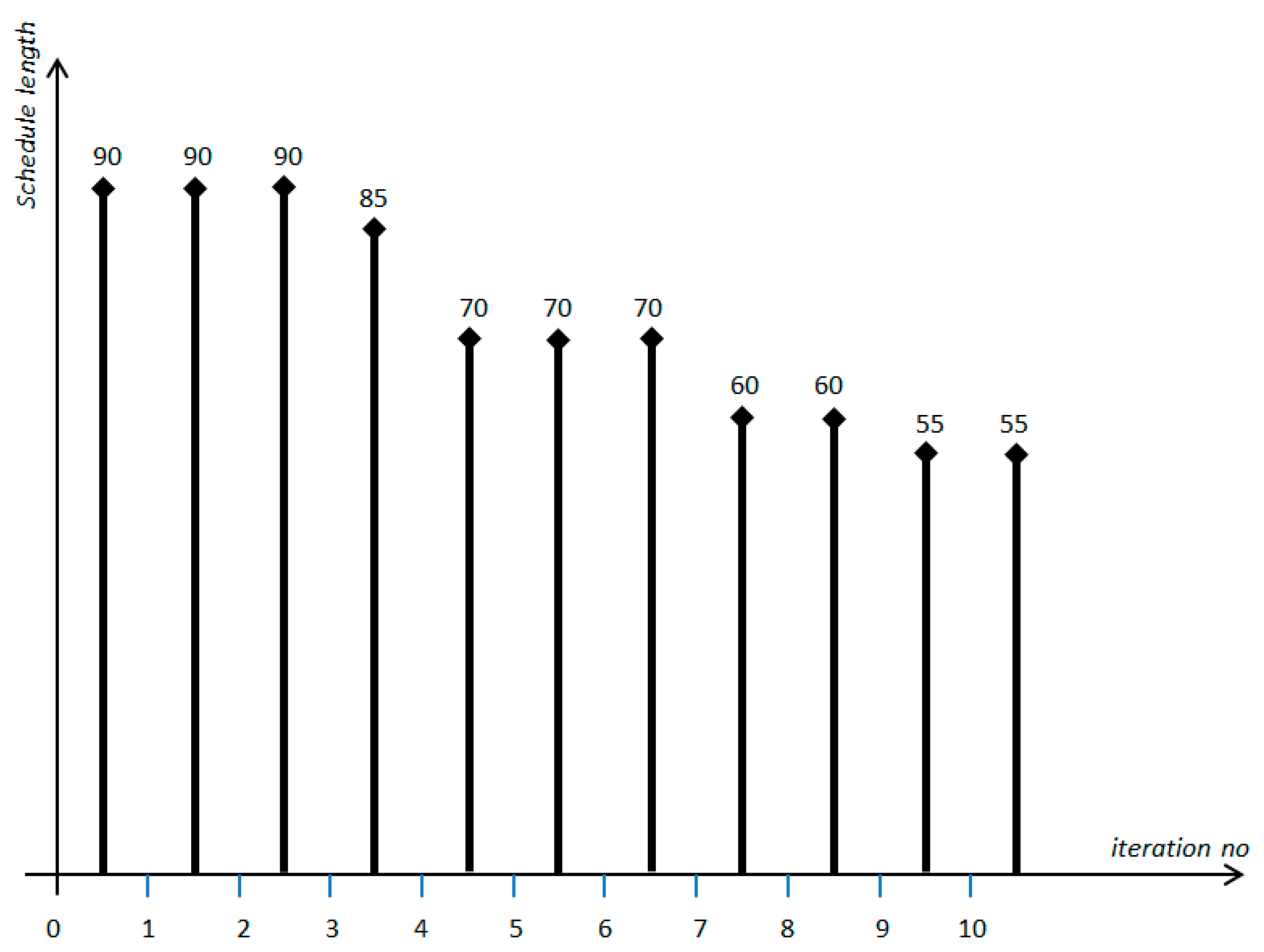
The performance of a search algorithm (including local search metaheuristics) is best analyzed by observing its convergence. The convergence of an algorithm is the ratio of the quality of the best solution found to the computation time. In the case of metaheuristic algorithms, it is convenient to study them in relation not to time but to the number of iterations of the main loop of the program. It can be assumed for simplicity that the best solution found so far is not lost during further computations. In the case of evolutionary algorithms, this requires the mechanism of elitism, according to which the best solution in a population is always transferred to the new population. Under this assumption, convergence is a discrete, non-decreasing function.

It is worth noting at this point that when solving problems of minimization of a given objective function, the quality of a solution is inversely proportional to the value of the objective function. In the next iteration of an algorithm, the best solution yields a smaller value of the objective function than the best solution in the previous iteration. Figure 3 shows an example of the convergence function for a scheduling problem.

In the classical way of using metaheuristic algorithms, the main emphasis is on the selection of the stopping criterion to

• Avoid interrupting computations during the exploration of a very promising area of potential solutions to the problem;
• Not to carry out computations when there is no chance to improve the best previously found solution (perhaps the optimal one).

Unlike the traditional approach, the stopping criterion proposed in this work mainly takes into account the energy aspect of the computations carried out.

2.2.3. Model of the Computational Task

For the purpose of this work, we assume that the convergence of the implemented computational task, i.e., an EA, is not known in advance. Thanks to the mechanisms built into the algorithm, we can only be sure that the current best solution is not worse than the previous one.

The computational task is iterative in nature. The size w of each iteration is fixed. The number of iterations no is unknown and will be determined after the computations are completed. The processing speed s_j of the processor in iteration $j, j=1,\dots , no$ is fixed and depends on the power used in iteration p_j, according to relation (2). This speed is determined before the iteration starts. The power $p_j, j=\mathrm{1,2},\dots ,no$ is limited in advance by a known value of the maximum power $P$. This means that the maximum speed of the operation in each iteration is also limited, up to some known value:

$$s_{max}=s_j\left(P\right)=\sqrt[3]{P}$$

(3)

Moreover, it is assumed that the processing speed of the processor, fixed for a given iteration, cannot be changed until the completion of the last operation in the iteration.

Let us now notice that assuming certain resource limits, i.e., energy $E (E>0)$ and time $T (T>0)$, are necessary for computations, it is very interesting to consider the problem of selecting a speed of computation at which the largest number of iterations will be performed within the computational task. This is because it is an obvious fact that, under a non-decreasing convergence function, a larger number of iterations in the algorithm leads to potentially better solutions. Assuming the same speed of computation in successive iterations of the computational task (and, consequently, constant power usage $p_j=p, j=\mathrm{1,2},\dots ,no$), as well as the same size of the computational task in each iteration, the corresponding optimization problem can be formulated as follows:

Maximize

$$no$$

(4)

Subject to

$$no·w·p^{2/3}\le E$$

(5)

$$no·w·p^{-1/3}\le T$$

(6)

$$0\le p\le P$$

(7)

It is easy to see that the largest number of iterations of the computational task will be obtained for:

$$p^{*}=\mathrm{m}\mathrm{i}\mathrm{n}\left(P,\frac{E}{T}\right)$$

(8)

whereas the maximum total number of iterations no* is given by the formulas:

$${no}^{*}=⌊\frac{T}{w}·{\left(\frac{E}{T}\right)}^{\frac{1}{3}}⌋ for \frac{E}{T}\le P$$

(9)

$${no}^{*}=⌊\frac{T}{w}·{\left(P\right)}^{\frac{1}{3}}⌋ otherwise$$

(10)

It should be stressed that the above analysis has been performed under several simplifying assumptions. In a general case, the execution of a computational task may involve a sequence of iterations of lengths unknown in advance, with each iteration at a potentially different processing speed. The possibility of controlling the processing speed of a particular iteration of the computational task will be used in the approaches discussed in Section 3.3.

2.3. Exemplary Scheduling Problem

As it is known, over the years, metaheuristic algorithms, in particular evolutionary algorithms, have been successfully applied to solving computationally hard scheduling problems. The main directions of research are aimed at improving their efficiency by using mechanisms that take advantage of the specificity of the problem being solved.

In EA implementations, to represent solutions to scheduling problems, some types of permutation coding are often used, through which the order of execution of jobs is most easily expressed. However, the intuitive simplicity of such a representation does not carry over to the ease of constructing corresponding genetic operators. This is because it is most often required that, as a result of using such operators, feasible solutions be obtained.

The innovation of the approach presented in this paper consists in the fact that a certain resource is simultaneously distributed between the procedure of solving a scheduling problem itself and the jobs being scheduled by this procedure. Thus, there is a natural coupling between the method and the solution generated by it.

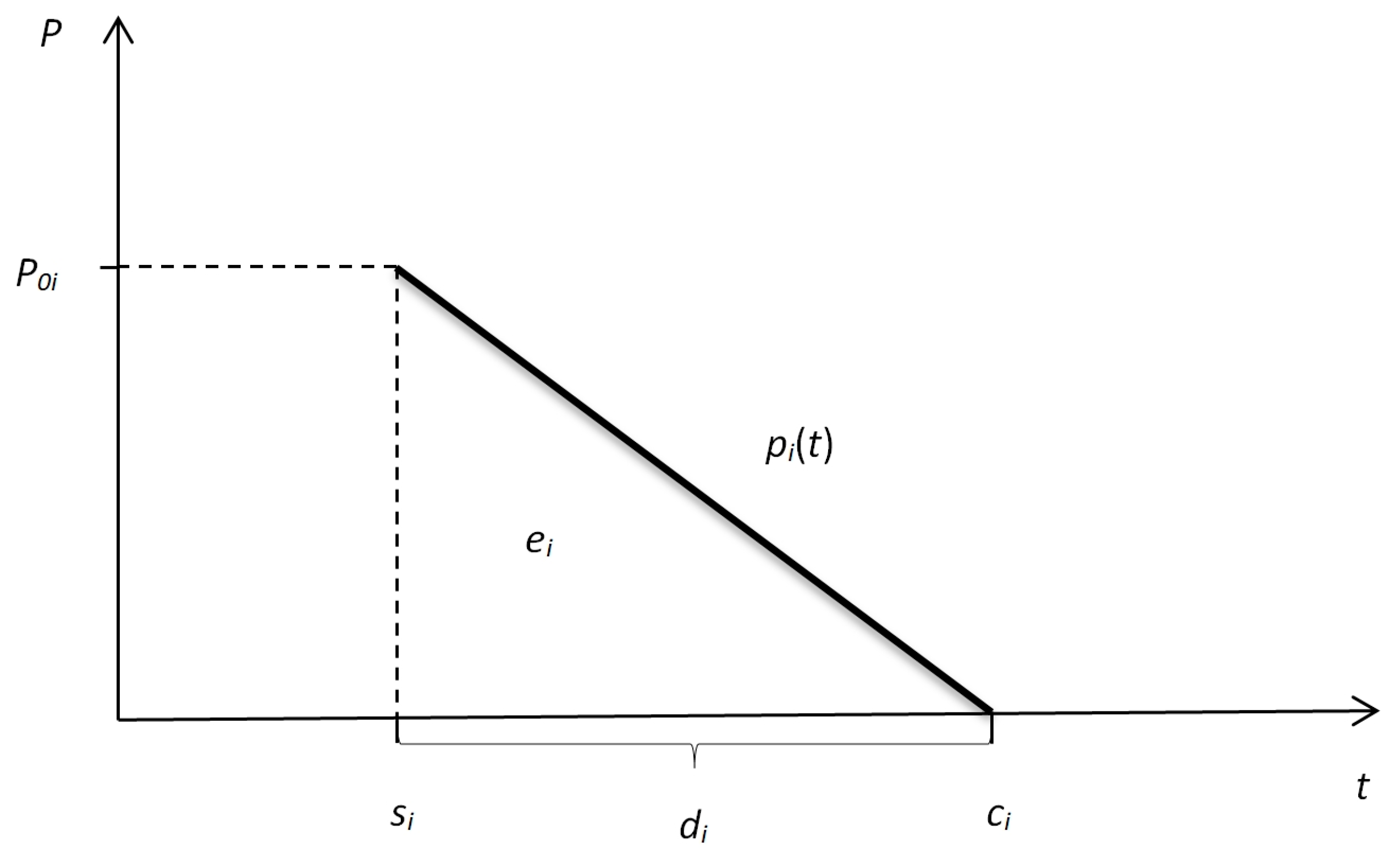
As an example of a scheduling problem, consider the problem of charging a fleet of drones powered by batteries of a certain capacity. We assume that these batteries are made using lithium-ion technology, which is typical for, e.g., EMVs. The time characteristic of the last stage of charging such batteries (see, e.g., [19]) shows that the power being used is a non-increasing function of the charging time and drops from a known initial value. As a result, the power demand decreases along with the charging rate of a battery. We assume that each battery is characterized by its capacity and its initial power demand, which, in general, can be different for different batteries. Battery charging time depends on the degree of its discharge, but let us assume that it is known in advance. To describe this situation, it is useful to apply a job model in which the job’s profile is characterized by a descending linear function with both the initial and the final values known. The final value corresponds to the power used at the end of the charging process. We additionally assume that the final value is equal to 0, i.e., after a battery has been fully charged, it requires no power anymore.

A general problem of this type was presented and discussed in [20]. Below, we formulate the problem in the form considered in this paper.

We assume that $n$ independent, nonpreemptable jobs are to be scheduled; each of them requires some amount of power for execution and consumes some amount of energy during processing. Charging job $i,i=\mathrm{1,2},\dots ,n$ is characterized by the amount $e_i$ of consumed energy (representing the size of the job), the initial power usage $P_{0i}$, and the power usage function $p_i\left(t\right)$. As mentioned before, the function $p_i\left(t\right)$ is assumed to be decreasing and linear, and $p_i\left(c_i\right)=0$, where $c_i$ is the finish time of job $i$, i.e., at the completion of the job, its power usage drops to 0. A graphic interpretation of the job model under the above assumptions is presented in Figure 4, where $s_i$ is the start time of job $i$.

Taking two points $(s_i,P_{0i})$ and $(c_i,0)$ of a linear function, we can easily derive the function formula. Consequently, the charging job model can be formally defined as:

$$p_i\left(t\right)=\left\{\begin{array}{c}0 for t<s_i\\ P_{0i}-\frac{P_{0i}}{d_i}\left(t-s_i\right) for s_i\le t\le c_i\\ 0 for t>c_i\end{array}\right.$$

(11)

From Figure 4, we can also observe that in the system of coordinates $p$ and $t,$ each charging job is graphically represented by a rectangular triangle of height $P_{0i}$ and length $d_i.$ The surface area of such a triangle defines the energy consumed by the charging job (i.e., the size of the job), according to Formula (12):

$$e_i=\frac{1}{2}{P}_{0i}{d}_i$$

(12)

And, consequently, knowing the size $e_i$ of job $i$ and its initial power usage $P_{0i}$, the processing time $d_i$ of the job can be calculated as:

$$d_i=2e_i/P_{0i}$$

(13)

Obviously, it has to be assumed that $\underset{i=1,\dots ,n}{\max }\left\{P_{0i}\right\}\le P$, where $P$ is the total amount of power, since otherwise no feasible schedule exists (at least one charging job cannot be executed). The specificity of the presented problem is that the charging jobs have fixed energy consumptions, and their execution order only affects time-based scheduling criteria.

The objective is to minimize the length of the schedule of the charging jobs under a limited amount of power. Let us stress that even if we assume an unlimited number of charging points (i.e., no limited discrete resource occurs), the problem requires a scheduling procedure since the available amount of power is not sufficient for performing all the jobs in parallel. Additionally, a deadline $D$ is imposed, i.e., the moment demanded for completing the execution of the entire set of jobs.

Taking schedule length as an optimization criterion has a very strong practical justification. While charging batteries, there is some emission of electromagnetic radiation [21], which can be disadvantageous, e.g., when there is a need for special protection in the immediate vicinity of the charging station.

It is also worth noting that the proposed model is adequate for the situation of military use of a drone swarm, where the deadline $D$ for the swarm’s readiness to undertake another mission is set, and in addition—in order to reduce the risk of remote detection of the charging station—the entire charging process should last as short as possible. In such a situation, it is justified to look for a schedule in which the last charging job ends at time $D$, while the first one starts as late as possible (in other words, the drone swarm charging process is initiated as late as possible).

3. Materials and Methods

3.1. Model of an Autonomous Charging Station

In this section, we present the concept of an autonomous charging station. It is supposed to charge a collection of electric vehicles (e.g., drones) with various battery capacities. The station is not connected to any power supply, and therefore it is forced to use local energy storage with limited power and energy. The problem of determining the order of charging jobs is not trivial due to their different characteristics and the limits of energy storage.

In the proposed model of the autonomous charging station, we make the following assumptions:

• The station consists of two modules: a computing one and an executive one;
• The computing module is equipped with a VSP processor made with CMOS technology;
• The result of the execution of the computational task performed by the computing module is a schedule of charging jobs, and the corresponding algorithm takes into account the adopted scheduling criterion;
• The computational task has to be finshed before the first charging job starts;
• The executive module performing energy charging jobs does not have a fixed limit of charging slots (theoretically, it is possible to charge any number of drones simultaneously);
• Both modules are powered by the same electric power source (energy storage) with a known capacity;
• There is an upper limit $P$ of power usage common to the computing and executive modules;
• The energy storage is not replenished either during computations or during the execution of the charging jobs.

Figure 5 shows the concept of an autonomous charging station.

3.2. Problem Formulation

In this section, we formulate the problem considered in this work more precisely. To this end, let us assume that the autonomous charging station meets the assumptions described in Section 3.1.

As already discussed, the computing module performs a single computational task. The executive module is to distribute energy among charging jobs. The computational task and the charging jobs apply to the same continuous, doubly-constrained, non-renewable resource, which is power, whose consumption over time is represented by energy. Both modules are driven by a common energy storage system. In the storage, the temporary available amount of power is limited by $P$, whereas $E$ is the constraint for its overall consumption (energy) (both $P$ and $E$ are positive).

The order of the charging jobs is not known in advance and has to be determined before the first job starts. The last charging job must end by the known deadline $D$. The processing speed of a computational task can be changed during its execution, and the time of its completion is unknown a priori. Moreover, let us notice that in the case of charging jobs described in Section 2.3, each schedule results in the same energy consumption, and the computing module only has an impact on the length of the schedule. Of course, it does not have to be the case in a more general practical situation.

The problem considered is to find:

• The allocation of power (and, consequently, the processing speed of the computational task) in each iteration, as well as the stopping criterion of the computational task.

So that

• The resulting schedule of charging jobs ends before the given deadline $D$ and has the minimum length.

Let us notice that the search for a feasible solution is pointless when, for a given instance of the problem, the total energy demand of all charging jobs exceeds its available amount $E$. Thus, we further consider only such instances in which the amount of energy in the storage is sufficient for executing all charging jobs.

3.3. Approaches

Let us now consider some situations for which various approaches to finding a solution to the problem can be proposed. In all of them, it is assumed that, for a given problem instance, an initial schedule of charging jobs is obtained by applying a simple heuristic algorithm. This can be, e.g., a list algorithm in which the order of charging jobs is defined according to, for instance, their non-increasing processing times.

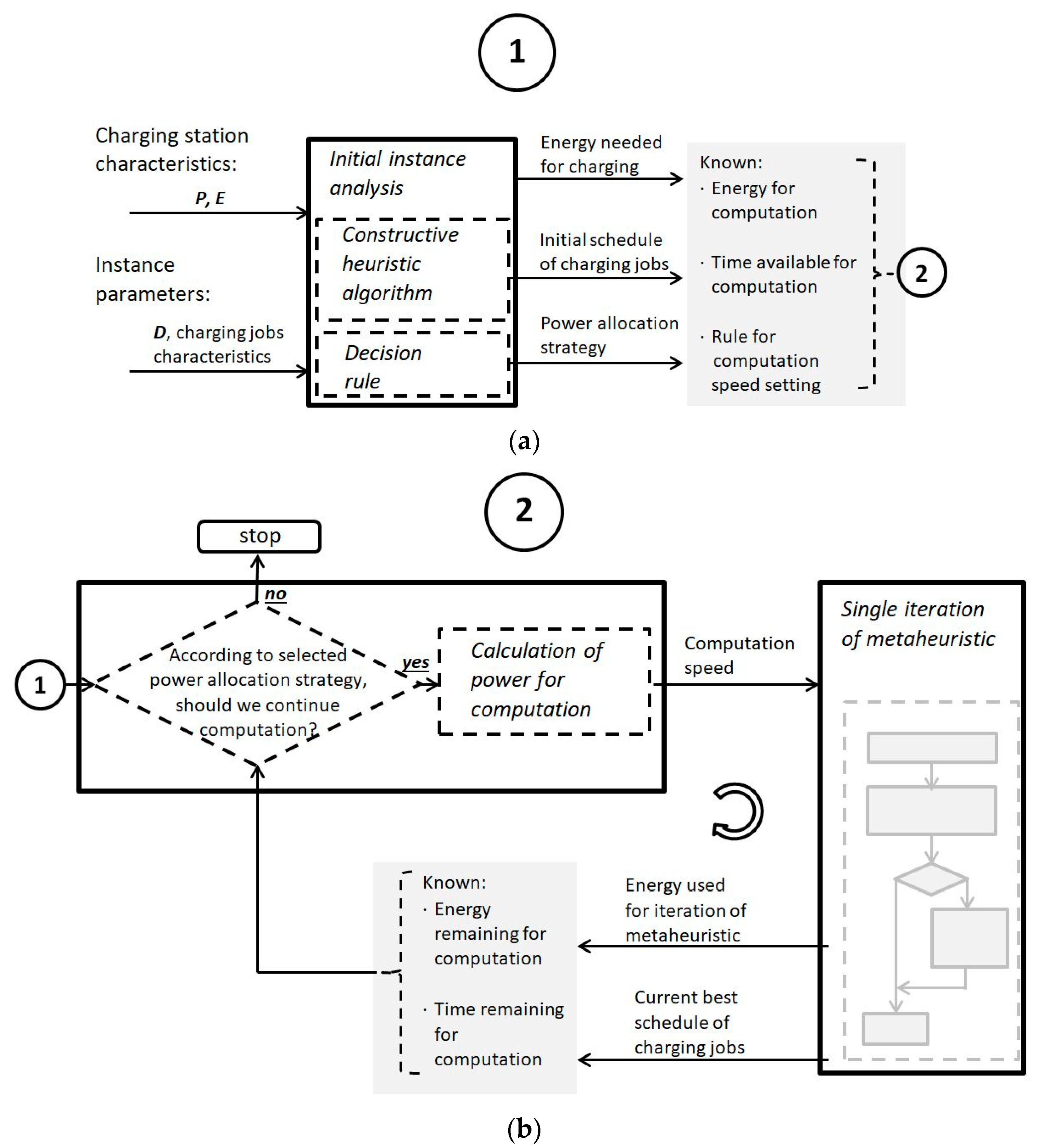
A graphical presentation of the general methodology and solution approach proposed in the paper is shown in two parts in Figure 6. Figure 6a illustrates the initialization phase, whereas Figure 6b presents the main loop of iterative computations.

3.3.1. Safe Approach

Let us first consider the case in which the initial schedule of charging jobs is feasible with respect to the assumed deadline $D$ and, additionally, there remains a certain non-zero reserve of time that can be allocated to the search for a shorter schedule. In such a situation, it is justified to use a so-called “safe approach”, in which the computational task is carried out as long as there are non-zero reserves of time and energy necessary for its execution. The computational task ends when at least one of those two resources—either time or energy—is exhausted.

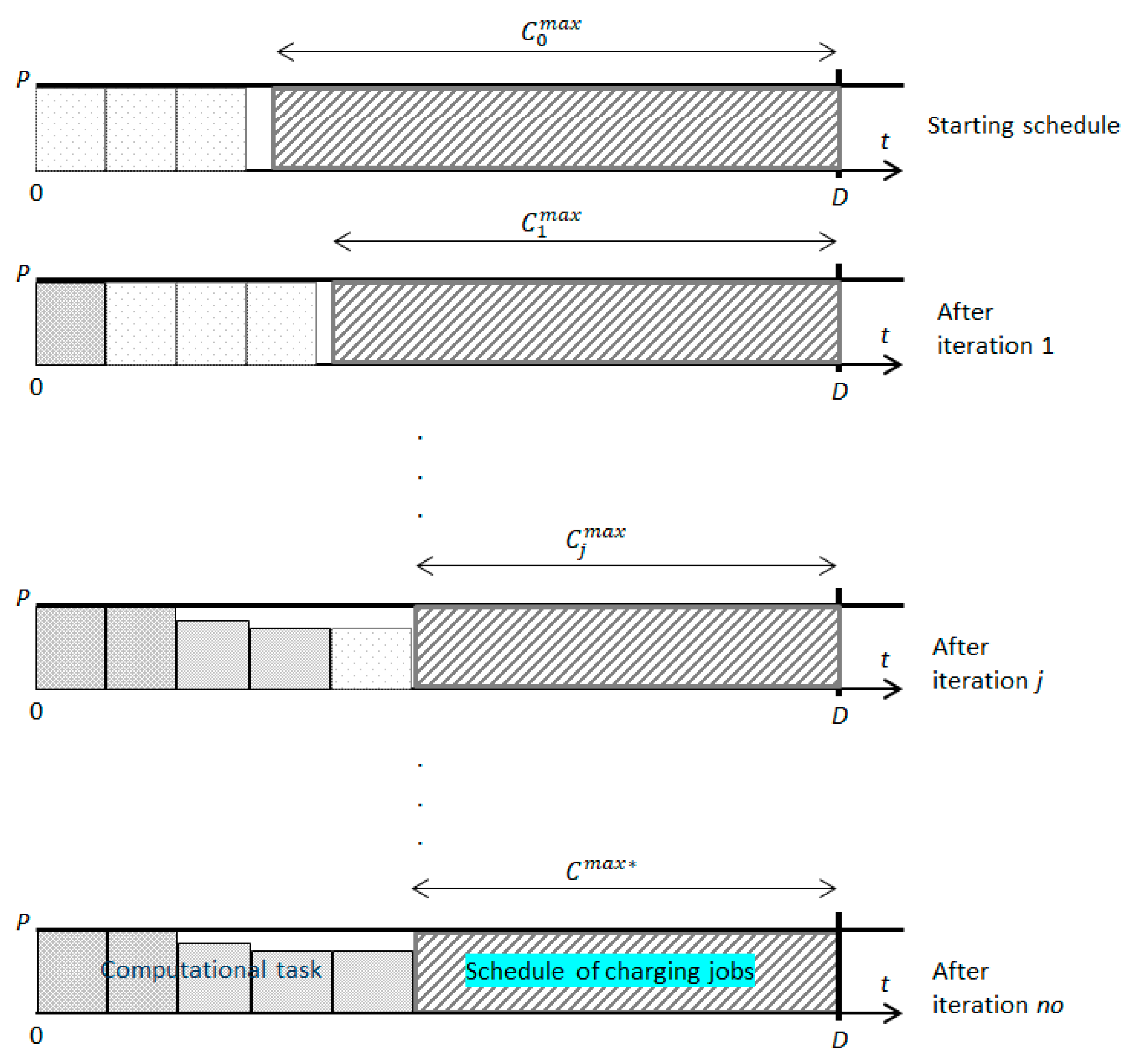
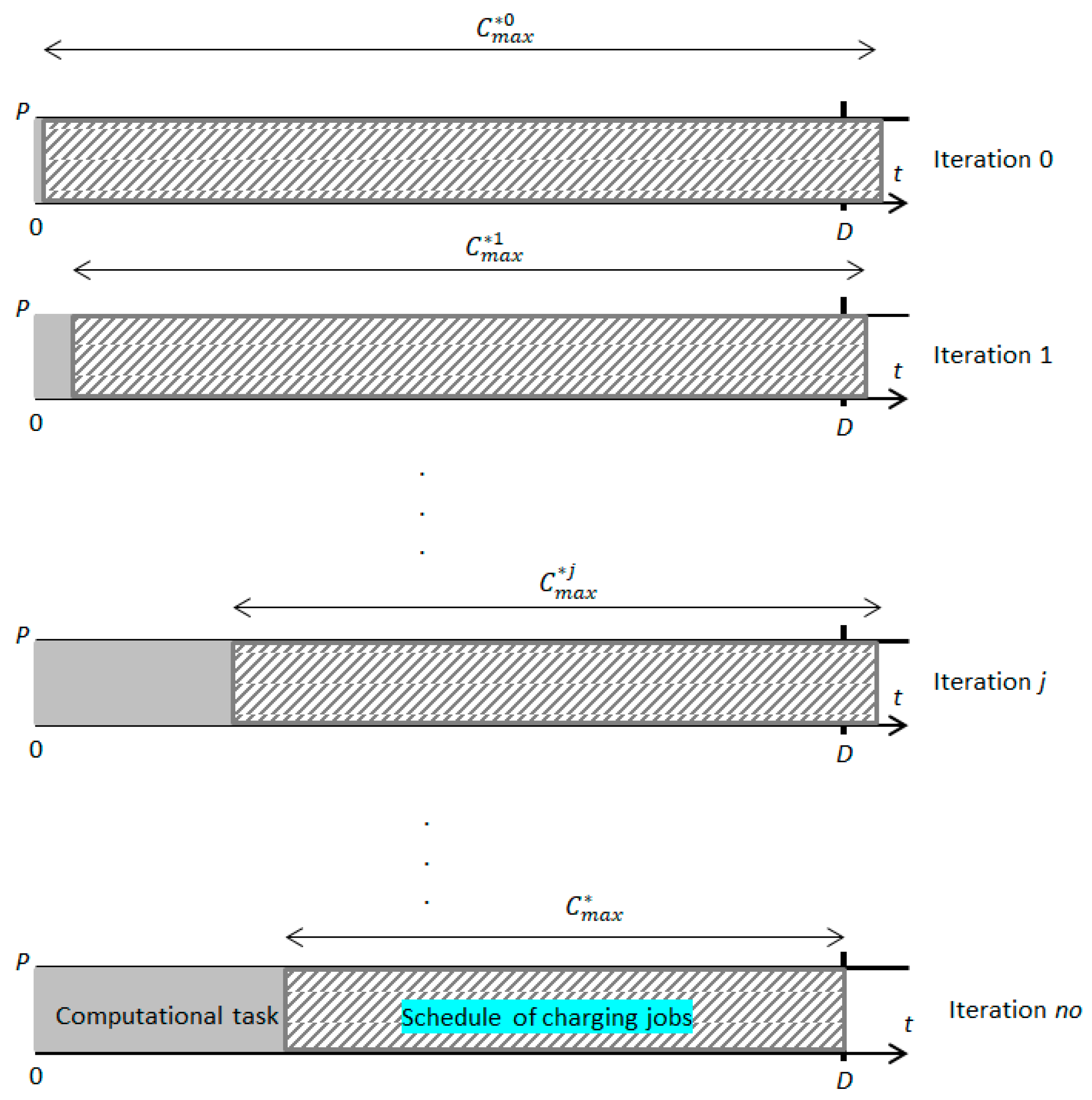
In this approach, the length of the schedule of charging jobs is improved by increasing the number of iterations of the EA algorithm (i.e., the computational task). The number ${no}^{*}$ of its iterations determined (based on Formulas (9) and (10)) before running EA takes into account the initial supply of time and energy for computations. If, during the operation of EA, such an initial schedule of length $C_0^{max}$ still remains the best, the computations will end after ${no}^{*}$ iterations without producing the expected effect—shortening the length of the initial schedule.

The situation is different if, in iteration $j\le {no}^{*},$ a schedule better than the best found so far is generated ${(C}_j^{max}<C_0^{max})$. This creates an additional reserve of time that can be used to increase the remaining number of EA iterations. To this end, Formulas (9) and (10) are applied again, taking into account the updated value of the remaining available computation time and the remaining amount of energy to be used. It is worth noting that if the calculated new number of iterations is derived from the constraint on energy (i.e., from Formula (9)), then an increase in the number of EA iterations can occur despite a reduction in their execution speed.

In Figure 7, Figure 8 and Figure 9, we present three situations that may occur under the safe approach: active time constraint, energy constraint, and both constraints. In the figures, $C_j^{max}$ is the length of the shortest schedule generated in iteration j, and $C^{max*}$ is the length of the final schedule found.

Figure 7 shows the situation where the initially determined number of EA iterations equal to three is, during computations—due to finding better schedules—increased to five. It is worth noting that because of the sufficient amount of energy available for computations, all the iterations can be performed at full speed (with full power usage).

Figure 8 illustrates the situation when, from the beginning of computations, the possible number of iterations was only affected by the limited amount of energy. The additional reserve of computation time (resulting from finding shorter schedules) enables an increase in the number of iterations under the condition that the computations simultaneously slow down.

In Figure 9, another situation is shown when, initially, the active constraint on power enabled the increase in the number of EA iterations only if an additional sufficient reserve of computation time appeared. During computations, further shortening of the generated schedules caused the constraint on energy to become active. Increasing the number of EA iterations was therefore possible only by slowing down the computations.

3.3.2. Aggressive Approach

An aggressive approach is characterized by a simple rule: the computational task is performed at full speed (i.e., with power usage $P$). The computations continue as long as the energy required for their execution is still available. The idea of this approach is an optimistic assumption that in the next iteration (or sequence of iterations), the newly found best schedule will be shortened by at least as much as the computations in this iteration (or iterations) lasted. For some instances of the considered scheduling problem, this approach can surely be successful. The final solution may satisfy the condition of completing the set of charging jobs before the deadline $D$, even when the initial solution has not met this condition. However, it is easy to see that this approach is unreasonable in the case of rapid convergence to solutions close to optimum. This is because in such a situation, carrying out further computations only consumes energy and time without shortening the best schedule found (see Figure 10). In an extreme situation, this can lead to exceeding the deadline $D$, even when the initial solution was feasible.

3.3.3. Aggressive Approach with Stopping

The aggressive approach to stopping is justified when the initial schedule goes beyond the given deadline $D$. This approach is very similar to the aggressive approach. The important difference is that in this case, computations are stopped if a schedule of the charging jobs finishing before the deadline $D$ has already been found. Although a further improvement in the quality of the schedule (i.e., a reduction in its length) is still possible, the computational task no longer continues. If a feasible solution is not found, computations end when energy is exhausted (see Figure 11).

4. Discussion

Let us now discuss some practical aspects of applying the approaches presented in Section 3.3.

As mentioned before, an initial schedule is generated first, as a result of a simple heuristic algorithm. Some preliminary computational experiments showed that a list algorithm in which the order of charging jobs was defined according to their non-increasing processing times gave very promising results.

Afterwards, one of the approaches proposed in Section 3.3 can easily be applied. The decision on which one to use can be based on knowledge of the particular instance’s specificity. Below, we discuss some useful hints for applying the approaches to practical problems.

Safe approach in practice

1.

We calculate the length and the energy consumption for the initial schedule of charging jobs.

2.

We calculate the remaining amount of energy that may be used for computations and the maximum computation time, taking into account two known values: the deadline $D$ and the total available amount of energy $E$.

3.

Based on the amount of energy and the computation time, we calculate the maximum possible power used for computations (i.e., the maximum speed of computations in order to perform as many iterations as possible) and run the evolutionary algorithm.

4.

After each generation of EA, we calculate the energy consumption and the length of the best schedule found and adjust the power needed for computations to those two calculated values.

5.

The computations are interrupted when we run out of either energy or time for further computations.

It is worth noting that in the basic version of the safe approach, the only criterion for selecting the speed of computations in the next iteration is to maximize the number of iterations that can be performed before the computations end due to a lack of resources (energy or time). However, it can be noted (see Figure 6 and Figure 7) that shortening a schedule does not always automatically result in increasing the number of iterations. This is the case when shortening a schedule does not guarantee enough time to perform an additional EA iteration. In such a situation, it seems rational to slow down the computations in such a way that it does not decrease the predetermined number of iterations but instead enables you to save a certain amount of energy.

Aggressive approach in practice

1.

We calculate the energy consumption for the initial order of charging jobs.

2.

We calculate the amount of energy remaining for computations.

3.

We perform the computational task at full speed as long as energy is still available.

Aggressive approach with stopping in practice

1.

We calculate the energy consumption for the initial order of charging jobs.

2.

We calculate the amount of energy remaining for computations.

3.

We perform the computational task at full speed until either the obtained solution is feasible with respect to deadline $D$ or we run out of energy.

The essence of the aggressive approach is to search for better schedules at the expense of the energy consumed, as long as there is enough energy to run the computations. This approach is not geared toward saving energy. An attempt to save energy is adding to the aggressive approach the stopping criterion proposed in the modified approach. A certain portion of the available energy can, in fact, be saved when this criterion becomes active.

Let us now include a discussion explaining the reasons why, despite formulating the three above approaches, we do not present any experimental results in this paper.

First of all, let us notice that we are unable to compare the approaches presented in the paper to any previous works. An autonomous charging station is an innovative model that has not been proposed in any paper before. The three approaches presented in the paper are possible options to be used in a case where such a station is in operation. Their novelty consists in the fact that they are designed for a situation never studied before in the field of edge computing and, as a result, to find solutions to an originally defined optimization problem. Consequently, they cannot be compared with any method previously published simply because no such methods exist.

On the other hand, let us also explain why we do not compare our three proposed approaches to each other. The reason is that each of them should be applied to another type of problem instance. The essence of the methodology proposed in the paper is an appropriate choice of one of the approaches to a particular practical situation. The result of a comparison among the three approaches would critically depend on the percentage of instances of a particular type in the set of test instances. Of course, in that context, it would be interesting to examine the frequency of the appearance of a particular instance type in practical situations. This, however, can be a direction for future research and, additionally, does not constitute a computational experiment in terms of comparing the efficiency of the presented approaches. The model we propose in the paper is a conceptual one, in which many parameters (the energy amount saved in the station, energy amounts in drones’ batteries, etc.) have the characteristics of random variables with unknown distributions.

Finally, we would also like to stress that the application of classical heuristic methods to a hard scheduling problem in the context of the presented model of an autonomous charging station is not a trivial task in itself. This follows from the fact that their common feature is performing computations at maximum speed, i.e., at maximum processor power usage. This fact prevents those methods from activating more saving (i.e., slower) computation modes in situations when they are needed. It could be hard to make a heuristic operate slower in order to save energy because it is more required somewhere else, e.g., for charging vehicles. Furthermore, among heuristic methods, we can distinguish between constructive heuristics and search heuristics (mostly metaheuristics). Classical constructive heuristics are characterized by computational time and the amount of energy consumed, which are dependent on the instance size. They usually operate quickly and consume little energy; however, when time and/or energy are strongly limited (or even critical) resources, they may not be able to generate a feasible solution. This would result in a lack of time or energy for charging the drones. On the other hand, permanently fixed time and energy consumption give no opportunity to lead computations towards finding a feasible solution. As concerns local search metaheuristics, their computational time and consumed energy can be controlled by setting relevant stop criteria. Still, classical stop criteria are usually time-related (e.g., total computational time, total number of iterations, total number of visited solutions, etc.) and do not take into account the amount of energy consumed during computations. As a result, a time-related stop criterion alone may be insufficient when energy is the more critical resource.

Summarizing, based on the above arguments, we maintain that designing heuristic algorithms for the problem formulated in the paper and comparing them on the basis of a computational experiment is not a trivial task. It requires further analysis and, probably, quite sophisticated approaches because of the specificity of the autonomous charging station.

5. Case Study Simulation of Dynamic Power Allocation

In this section, we present a numerical example of the methodology proposed in the paper. The example corresponds to the safe approach described in Section 3.3.1, in which it is allowed to change the power allocation during computations. Let us recall that the dynamic approach (Section 3.3.2) or its version with stopping (Section 3.3.3) always use the maximum available amount of power. In the simulation given below, we demonstrate how dynamic adjustment of the processor speed can result in the growth of the number of iterations of an EA algorithm and, ipso facto, can help find a better (i.e., shorter) schedule for the charging tasks. As computational time and the amount of energy consumed for computations are both functions of the amount of power used by the processor, we consider three variants:

(a)

a fixed allocation of the maximum available power to the processor, which corresponds to a fixed maximum possible processing speed;

(b)

a fixed allocation of power to the processor equal to 20% of the maximum available power amount, which corresponds to a fixed slight processing speed;

(c)

a dynamic power allocation, which corresponds to a variable, is adjusted to a particular situation’s processing speed.

Based on Formula (1), where it is assumed that $\alpha =3,$ the following equations are immediate:

–

The processing speed $s$:

$$s=p^{1/3}$$

(14)

–

Time $t$ of performing a single EA iteration of size $w$:

$$t=w·p^{-1/3}$$

(15)

–

Energy $e$ consumed within the iteration:

$$e=w·p^{2/3}$$

(16)

Let us now list the assumptions made for the presented example:

• The initial schedule length (e.g., found by a constructive heuristic): 90;
• The EA convergence: given in the example in Figure 3;
• The size of a single EA iteration (measured as the number of processor instructions executed within the iteration): 10;
• The maximum available amount of power: 1;
• The total available amount of energy (including the energy needed for charging drones): 150;
• The amount of energy available for computations (excluding the energy for charging drones): 50;
• Deadline (time limit for charging): 140.

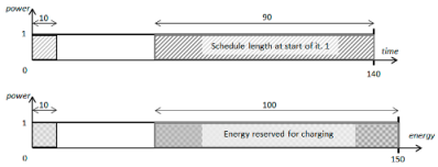
Variant a.

In the first variant, we obtain:

–

A fixed power amount used for computations during each iteration: $p=1$;

–

The processing speed in each iteration (from Formula (14)): $s=1$;

–

The time of computation in each iteration (from Formula (15)): $t=10$;

–

The amount of energy consumed for computations in each iteration (from Formula (16)): $e=10$;

The computations go as follows:

Iteration 1:

Iteration 2:

Iteration 3:

Iteration 4:

Iteration 5:

STOP—further iterations of EA are not possible due to the exhaustion of energy needed for computations.

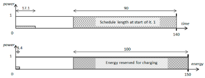
Variant b.

In the second variant, we obtain

–

A fixed power amount used for computations during each iteration: $p=0.2$;

–

The processing speed in each iteration (from Formula (14)): $s=0.585$;

–

The time of computations in each iteration (from Formula (15)): $t=17.1$;

–

The amount of energy consumed for computations in each iteration (from Formula (16)): $e=3.42$;

The computations are the following:

Iteration 1:

Iteration 2:

Iteration 3:

Iteration 4:

STOP—further iterations of EA are not possible due to the exhaustion of time needed for computations.

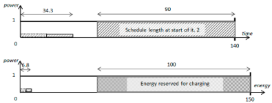
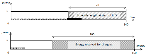
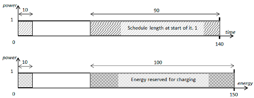
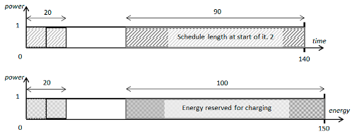
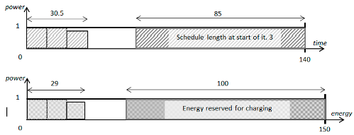
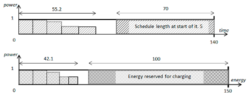
Variant c.

In the third variant, the power amount used by the processor is calculated dynamically from Formula (8), taking into account the current amounts of time and energy available for computations at the start of an iteration. The processing speed, the computational time, and the energy consumed by computations can vary, and in each iteration they are calculated from Formulas (14)–(16) correspondingly for the power usage defined for this iteration. Below, we present the computations in successive iterations.

Iteration 1: $p=min\left(1;\frac{50}{50}\right)=1$, $t=10, e=10$

Iteration 2: $p=min\left(1;\frac{40}{40}\right)=1$, $t=10, e=10$

Iteration 3: $p=min\left(1;\frac{30}{35}\right)=0.85$, $t=10.5, e=9$

Iteration 4: $p=min\left(1;\frac{21}{39.5}\right)=0.53$, $t=12.34, e=6.56$

Iteration 5: $p=min\left(1;\frac{14.4}{27.1}\right)=0.53$, $t=12.34, e=6.56$

Iteration 6: $p=min\left(1;\frac{7.8}{14.8}\right)=0.53$, $t=12.34, e=6.56$

STOP—further computations are not possible due to the lack of energy and time.

$$p=min\left(1;\frac{7.8}{14.8}\right)=0.53, t=12.34, e=6.56$$

In the above case study, we have shown that a dynamic allocation of power to the processor and, as a result, varying the processing speed during computation can improve the schedule of the charging tasks. The advantage of dynamic power allocation follows from the fact that it enables taking into account new, better solutions to the charging task scheduling problem found during computations. The strategies based on a fixed power usage, defined at the start of computations, do not have this feature. Let us also note that the strategy of maximum power allocation (variant a) is adequate in a situation with practically unlimited amounts of energy available for computations, whereas the strategy of a small processing speed (variant b) is reasonable in the case when there is a large amount of spare time until the end of the process of charging the drones. Those two strategies may, however, easily fail when the constraints on time and energy are both restrictive.

6. Conclusions

In this paper, a problem from the field of edge computing has been considered. An innovative model of a so-called autonomous charging station has been proposed. The station consists of a computing module, whose job is to solve the problem of scheduling charging jobs, and an executive module, whose job is to perform the jobs already scheduled. Both modules are driven by a common power source with limited power usage and energy consumption. An evolutionary algorithm is designed to construct a schedule of charging jobs. The problem is to define the speed of the EA execution in order to find a schedule of charging jobs having the minimum length and meeting the given deadline under power and energy constraints. Three possible approaches to attacking the problem—a safe approach, an aggressive approach, and an aggressive approach with stopping—have been proposed and discussed. The approaches can be generalized to various other cases, including, e.g., those in which the order of execution of the charging jobs affects not only the schedule length but also the overall energy consumption. A numerical example included in the paper shows that a dynamic adjustment of the processor speed can result in a better schedule for the charging tasks.

Future research on that topic can go in several different directions, including generalizations of the problem itself, modifications of the proposed autonomous charging station model, analyzing various computing algorithms (e.g., other metaheuristics), considering miscellaneous scheduling problems, or taking into account scheduling criteria other than the schedule length. As mentioned in Section 4, a very challenging topic would be developing specialized heuristic methods dedicated to the environment of the autonomous charging station. Such methods could then be compared on the basis of specially designed computational experiments. Another interesting direction is to involve quantum algorithms in research as they begin to obtain better and better results for various optimization models, including scheduling problems.