
Static and Dynamic Electrical Models of Proton Exchange Membrane Electrolysers: A Comprehensive Review


Abstract
:1. Introduction
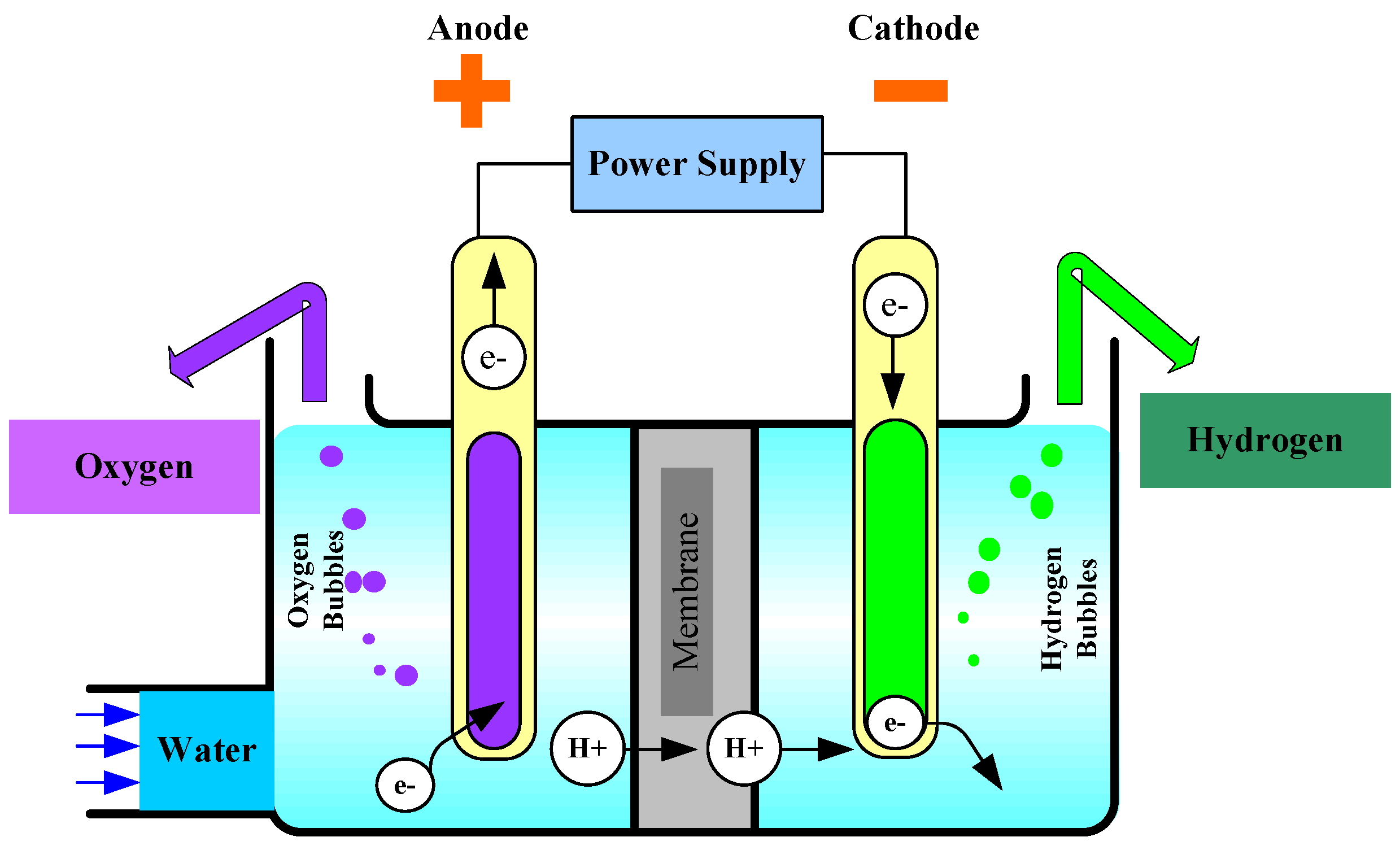
2. Fundamental Principles of Water Electrolysis
- change in the reaction enthalpy for this endothermic reaction [;
- Stoichiometric factor for product and reactant;
- : the stoichiometric factors;
- enthalpies of formation of the products [;
- enthalpies of formation of the reactants [.
- change in Gibbs free energy or free enthalpy of reaction [];
- T: system temperature [;
- molar change in entropy [];
3. Electrical Models
3.1. Steady-State Methodology
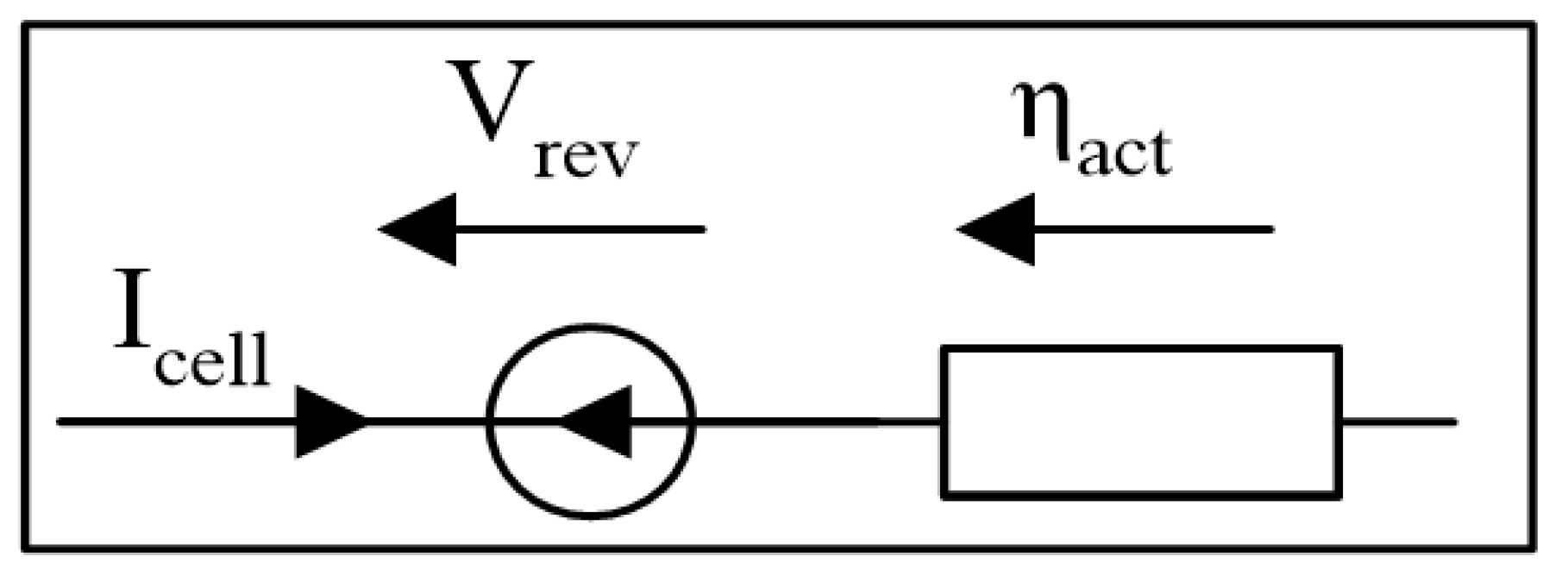
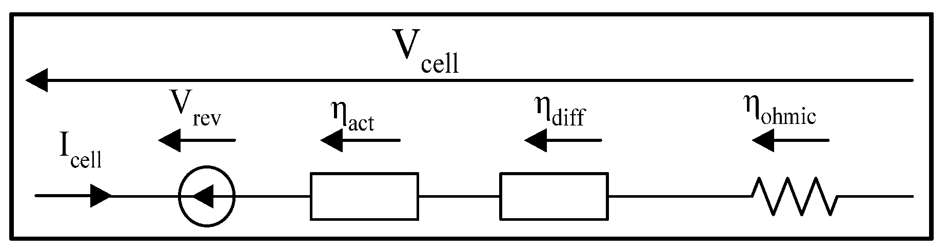
3.1.1. Semi-Empirical Models
- cell voltage [V];
- reversible voltage [V];
- : activation overvoltage [];
- ohmic overvoltage [V];
- : diffusion Overvoltage [].
Reversible Voltage
- F: Faraday’s constant [];
- reversible voltage at standard conditions [V];
- universal gas constant (8.314) [];
- hydrogen pressure [bar];
- oxygen pressure [bar];
- reference pressure [bar];
- n: number of moving electrons in the chemical reaction (n = 2);
- Gibbs Free Energy at standard condition [].

| Reversible Voltage | Equation | Ref. |
|---|---|---|
| (9) | [12,17,18,19,20,21,22,23] | |
| (10) | [23,24,25] | |
| (11) | [26] | |
| (12) | [12,27] | |
| (13) | [12,23,28,29,30,31,32] |
- T: system temperature [];
- reversible voltage (temperature-dependent equations) [V].
- Gibbs Free Energy at standard condition [];
- n: number of moving electrons in the chemical reaction (n = 2);
- anode reversible voltage [V];
- cathode reversible voltage [V];
- anode Gibbs Free Energy at standard condition () [];
- cathode Gibbs Free Energy at standard condition () [].
Activation Overvoltage
| Activation Overvoltage | Equation | Ref. |
|---|---|---|
| (20) | [33,34,35] | |
| (21) | - | |
| (22) | [3,18,19,36,37] | |
| (23) | [17,20,25,28,38,39,40] | |
| (24) | [12,21,22,31,41,42] | |
| (25) | [26,27,43] | |
| (26) | [23] |
- cell current density [];
- the leakage current density due to crossover [];
- exchange current density at electrodes [];
- charge transfer coefficient [];
- activation overvoltage at both electrodes [V];
- T: system Temperature [];
- F: Faraday’s constant [];
- k: refers to anode (an) or cathode (cath);
- concentrations of the reaction product and reactant in the vicinity of the electrode [];
- concentrations of the reaction product and reactant in the solution [].
- global transfer coefficient [];
- total activation overvoltage [];
- anode charge transfer coefficient [];
- cathode charge transfer coefficient [].
Ohmic Overvoltage
| Conductivity | Equation | Ref. |
|---|---|---|
| (30) | [17,20,21,29,31,36,40,41,42,46] |
- membrane overvoltage [V];
- electronic overvoltage [V];
- electronic resistance [];
- L: length of the path of the electrons [cm];
- : electrode material resistivity [m];
- the electrode cross-sectional area [];
- Ionic resistance [];
- : thickness of the membrane [cm];
- : conductivity of the membrane [];
- T: temperature of the cell [K];
- : hydration rate [−];
- active surface area [].
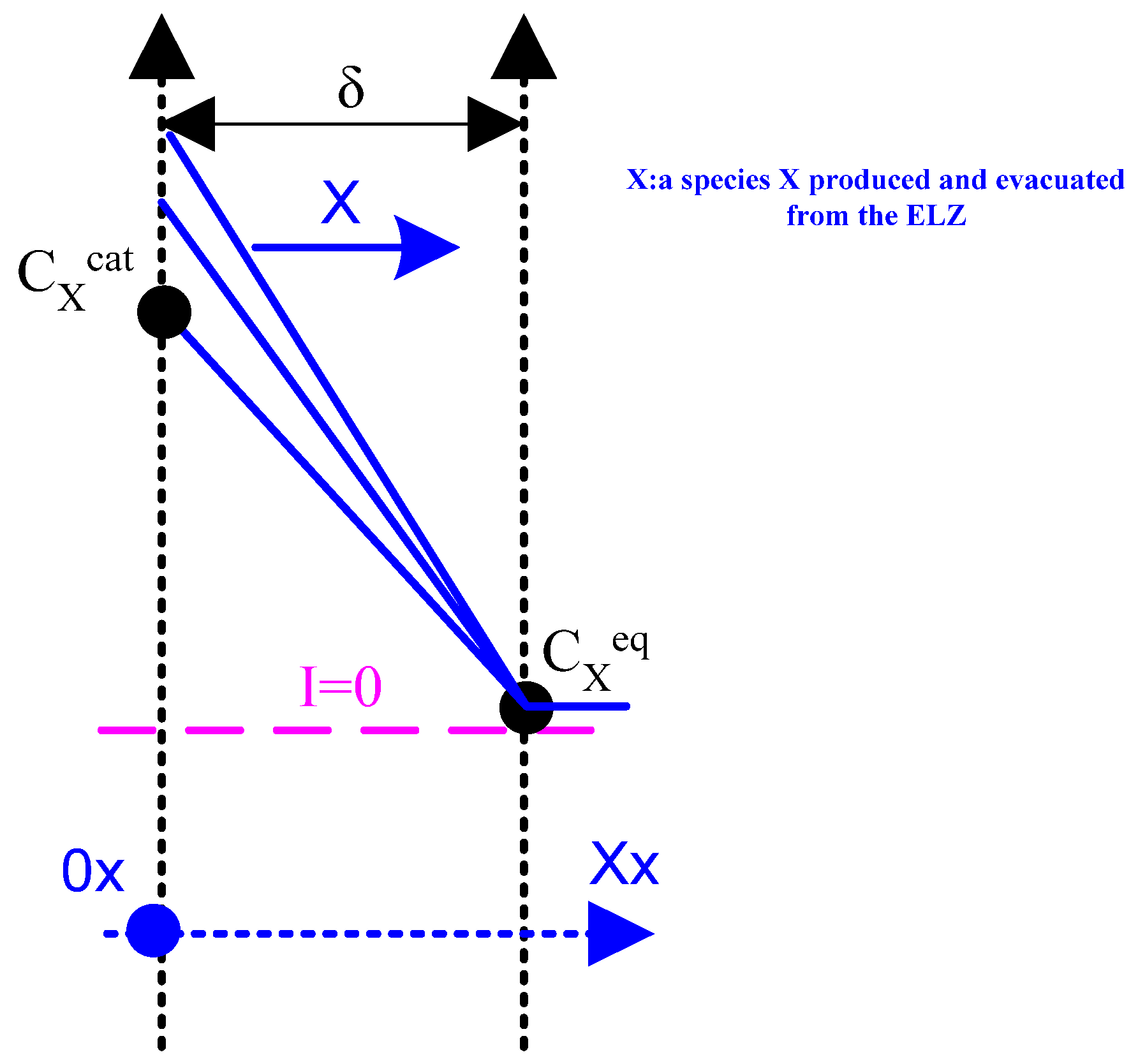
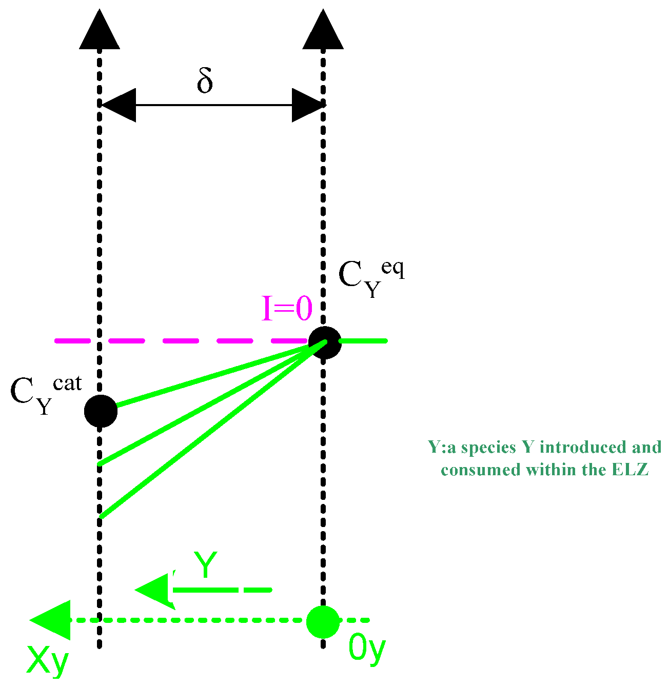
Diffusion Overvoltage
| Situation | Species | Formula | Equation |
|---|---|---|---|
| Case of a species x produced and evacuated from the electrolyser | and | (35) | |
| Case of a species y introduced and consumed within the electrolyser | (36) |
- stoichiometric coefficients of the species x and y. [];
- concentrations of species x and y, at the catalytic sites (cat is stand for catalytic);
- diffusion length [m];
- diffusion coefficients of the species x or y ;
- cell current [];
- A: active surface area [];
- diffusion limit currents [A];
- concentrations in the channel [], determined from the ideal gas law. [].
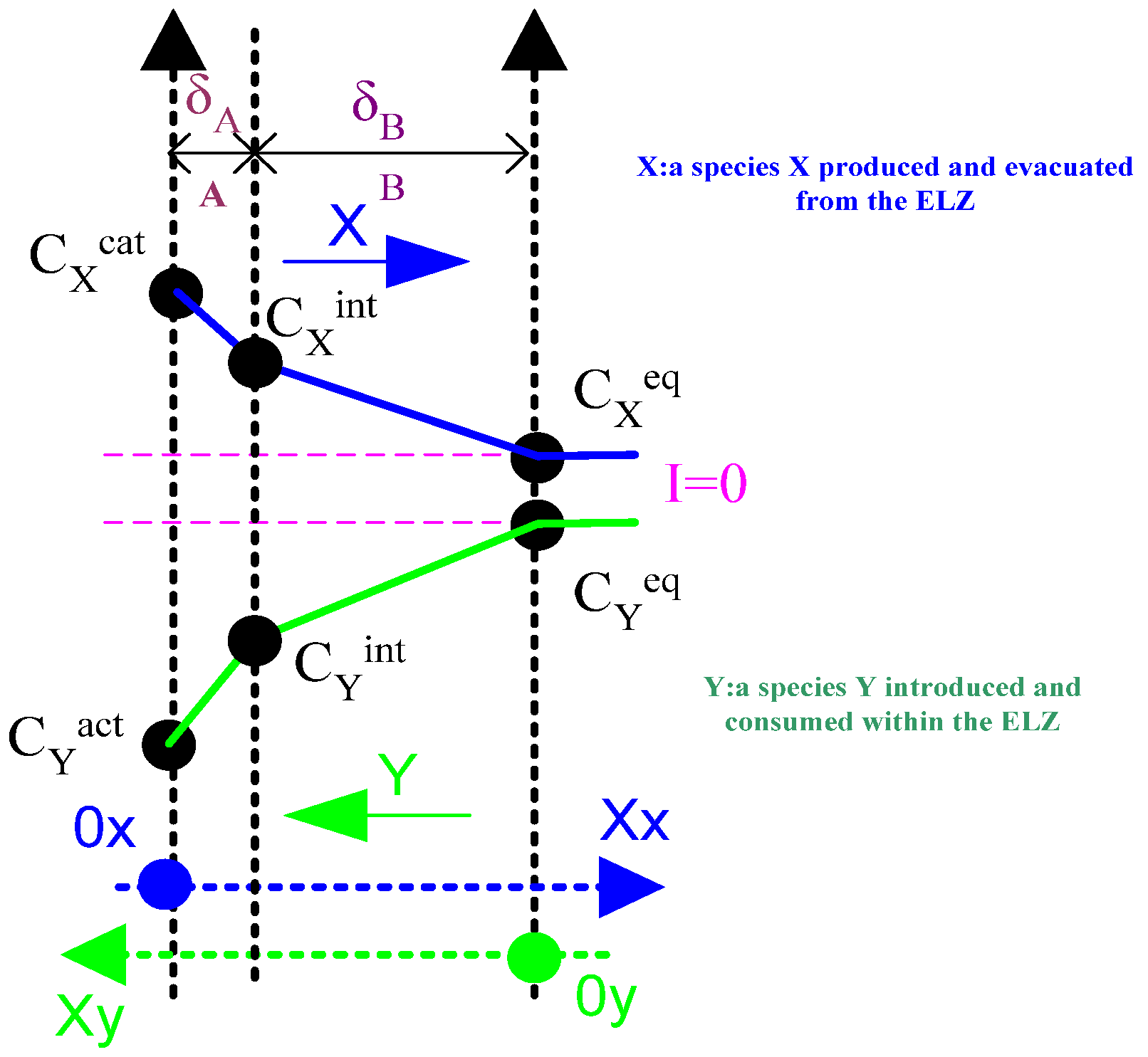
| Situation | Species | Formula | Equation |
|---|---|---|---|
| Case of a species x produced and evacuated from the electrolyser | and | | (37) |
| Case of a species y introduced and consumed within the electrolyser | | (38) |
- diffusion length of zones A and B [m];
- , diffusion limit currents effective respectively in zones A and B [A];
- diffusion limit current effective in zone A in the case of operation of the electrolyser in the opposite mode if there was only one zone [A];
- effective diffusion coefficients for zones A and B [].
Impact on the Voltage
Summary of the Static Approach
3.1.2. Empirical Models
- Fitting parameters.
| Empirical Electrochemical Models | Electrolysis Technology | Equation | Ref. |
|---|---|---|---|
| Alkaline | (49) | [43,48] | |
| Alkaline | (50) | [49] | |
| Alkaline | (51) | [50] |
- ,, ,, s, , and are constants obtained from the experimental data;
- P is the pressure of system [bar];
- is the cell current [A];
- temperature dependence of the parameters and was gained by fitting with a second-order polynomial.
3.2. Faraday Efficiency
- molar flow of hydrogen [];
- current efficiency [−].
- A: cell area [];
- empirical coefficients.
3.3. Dynamic Methodology
3.3.1. Large Signal Dynamic Models
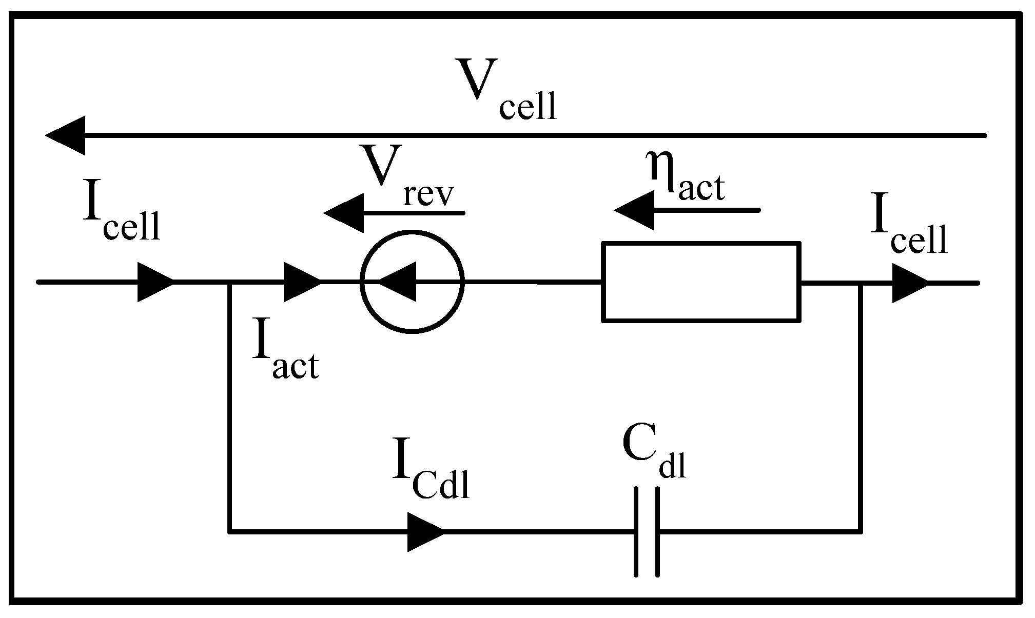
3.3.2. Dynamics of Activation Phenomena
- : capacitive current of the electrochemical double layer [A];
- : double layer capacitance [F].
- d: distance between the electrode and the electrolyte [m];
- ε: electrical permittivity [];
- : active surface of electrode [].
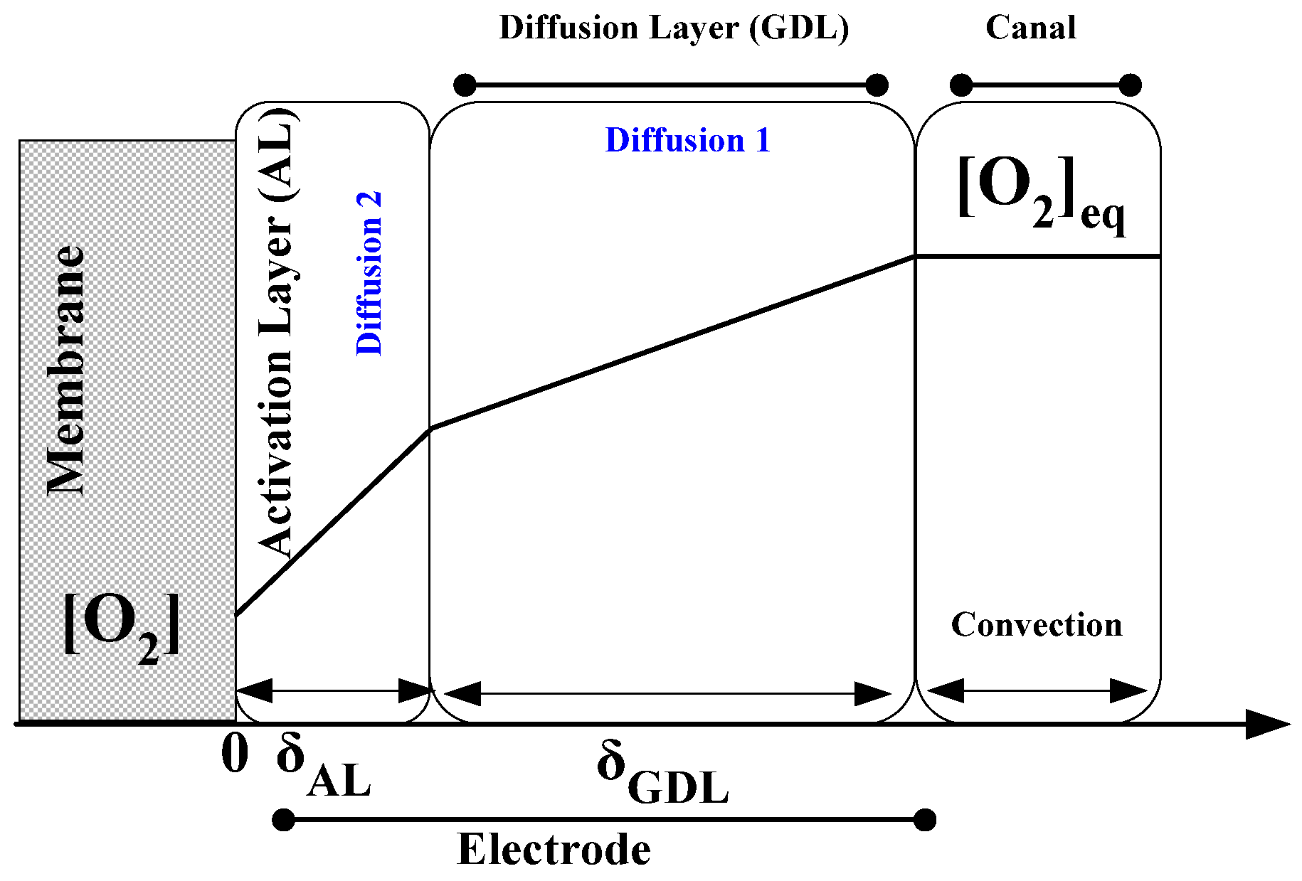
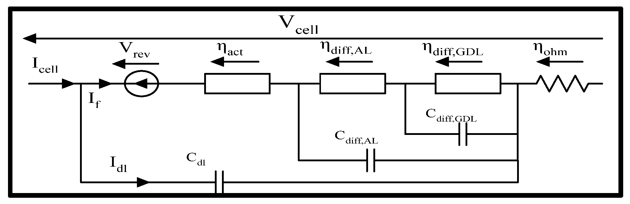
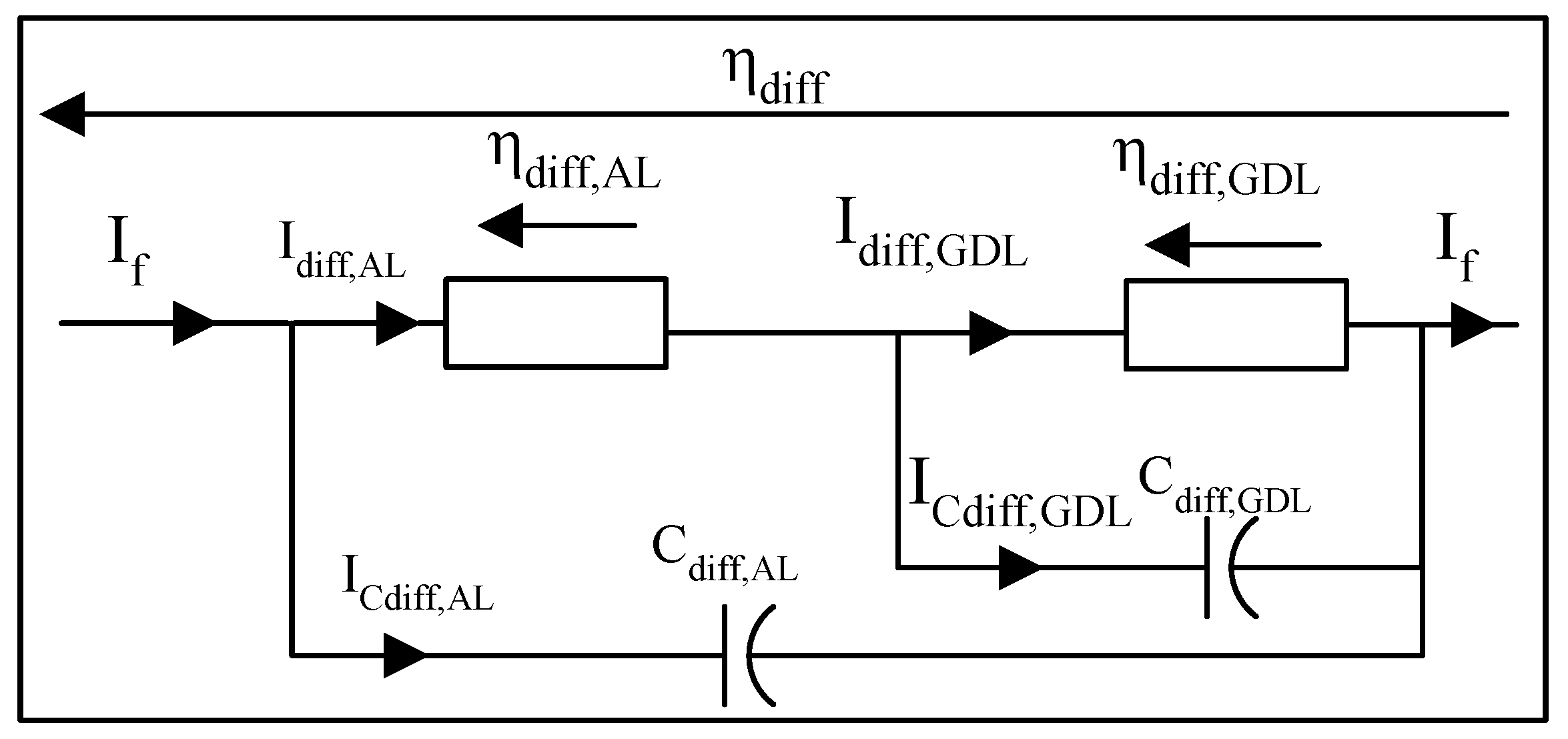
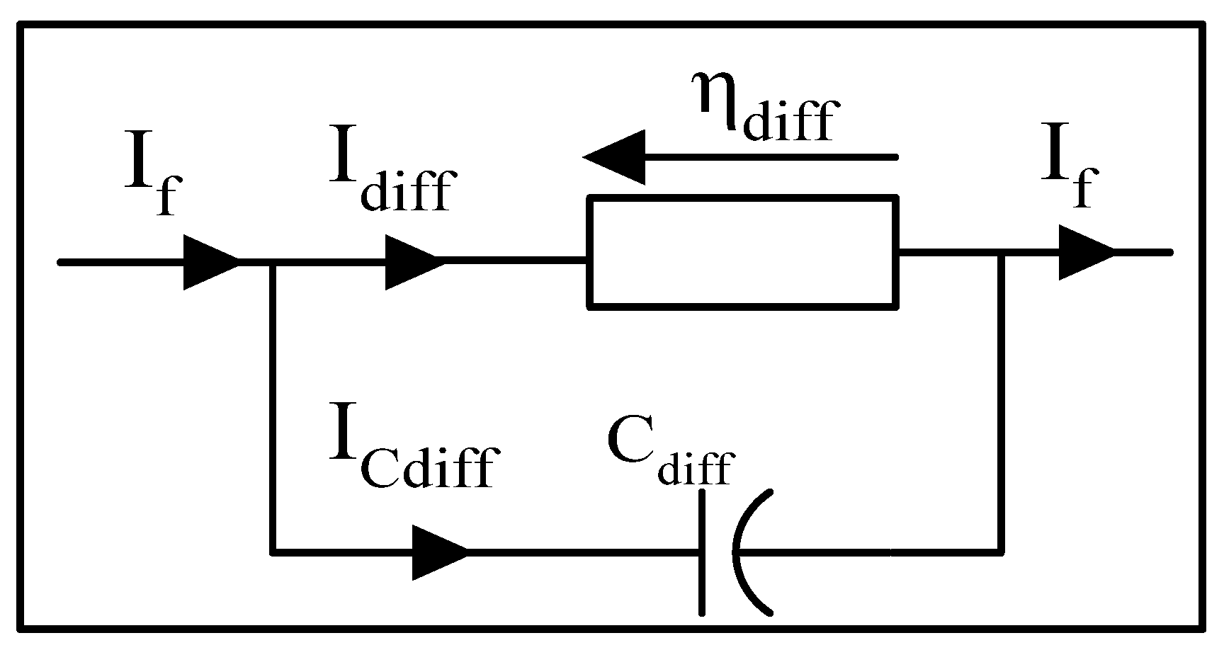
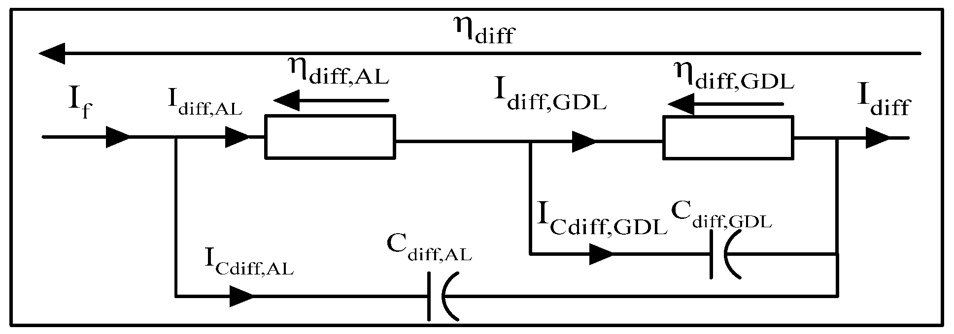
3.3.3. Dynamics of Diffusion Phenomena
- The first model adopts a single equivalent diffusion layer.
- The second model adopts two distinct diffusion layers, one for the Gas Diffusion Layer and another for the Activation Layer.
Dynamic model of diffusion phenomena with a single equivalent layer
- identified experimentally ;
- diffusion resistance ;
- capacitor of the diffusion phenomena [F];
- : diffusion curent [A];
- : effective diffusion coefficient [];
- diffusion length [m].
Dynamic model of diffusion phenomena with double equivalent layer
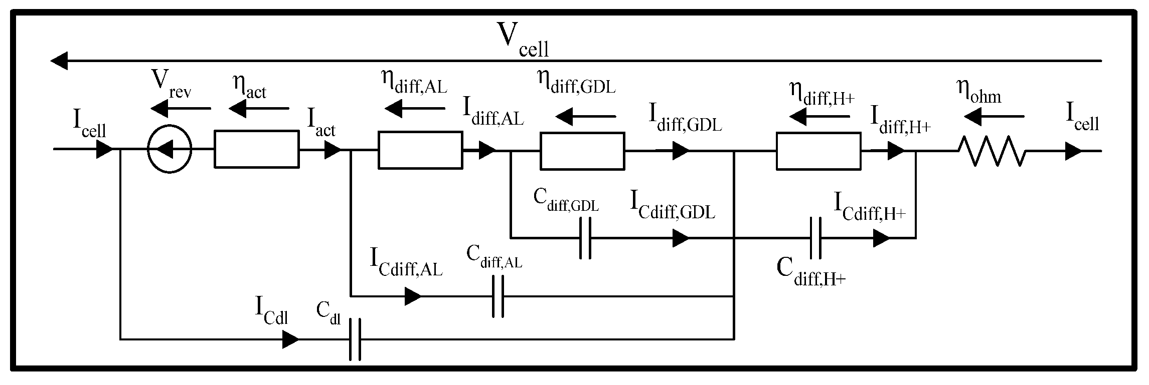
3.3.4. Summary of Large Signal Dynamic Models
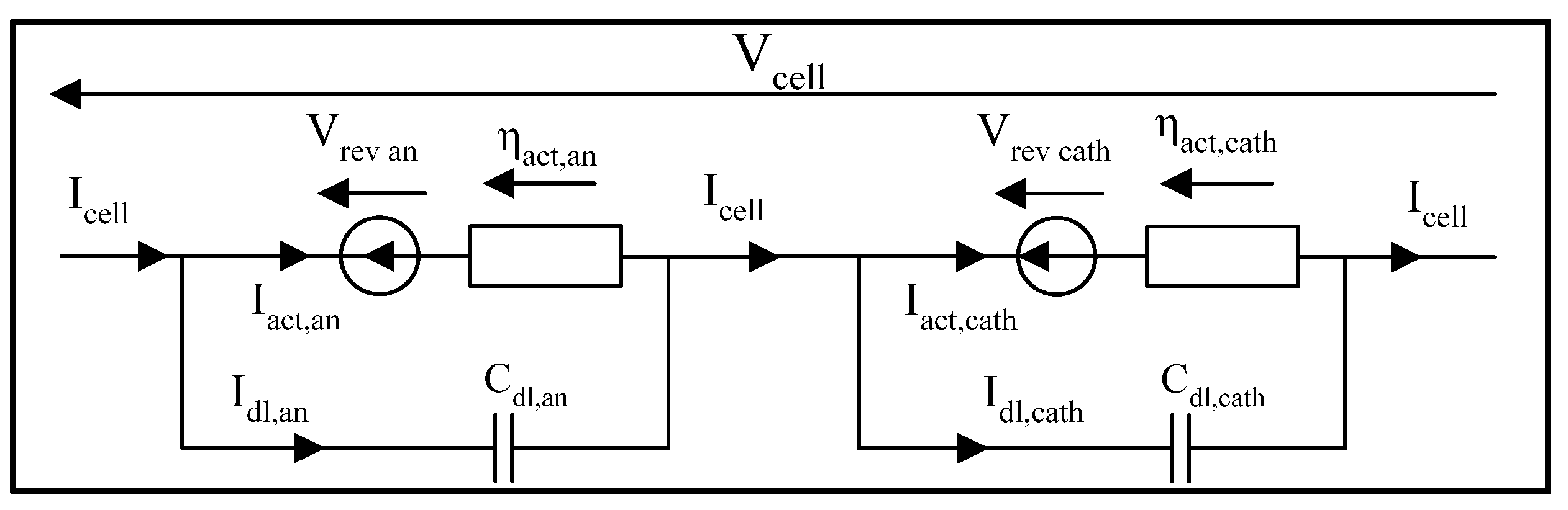
- The dissociated or non-dissociated electrodes;
- The proton transfer;
- The number of diffusion layers (AL, GDL);
- The consideration of parasitic phenomena.
3.3.5. Small Signal Dynamic Model
- is typically 0.5;
- : takes values between 0.7 and 1;
- is typically 1;
- take quite varied values between 0.3 and 1.
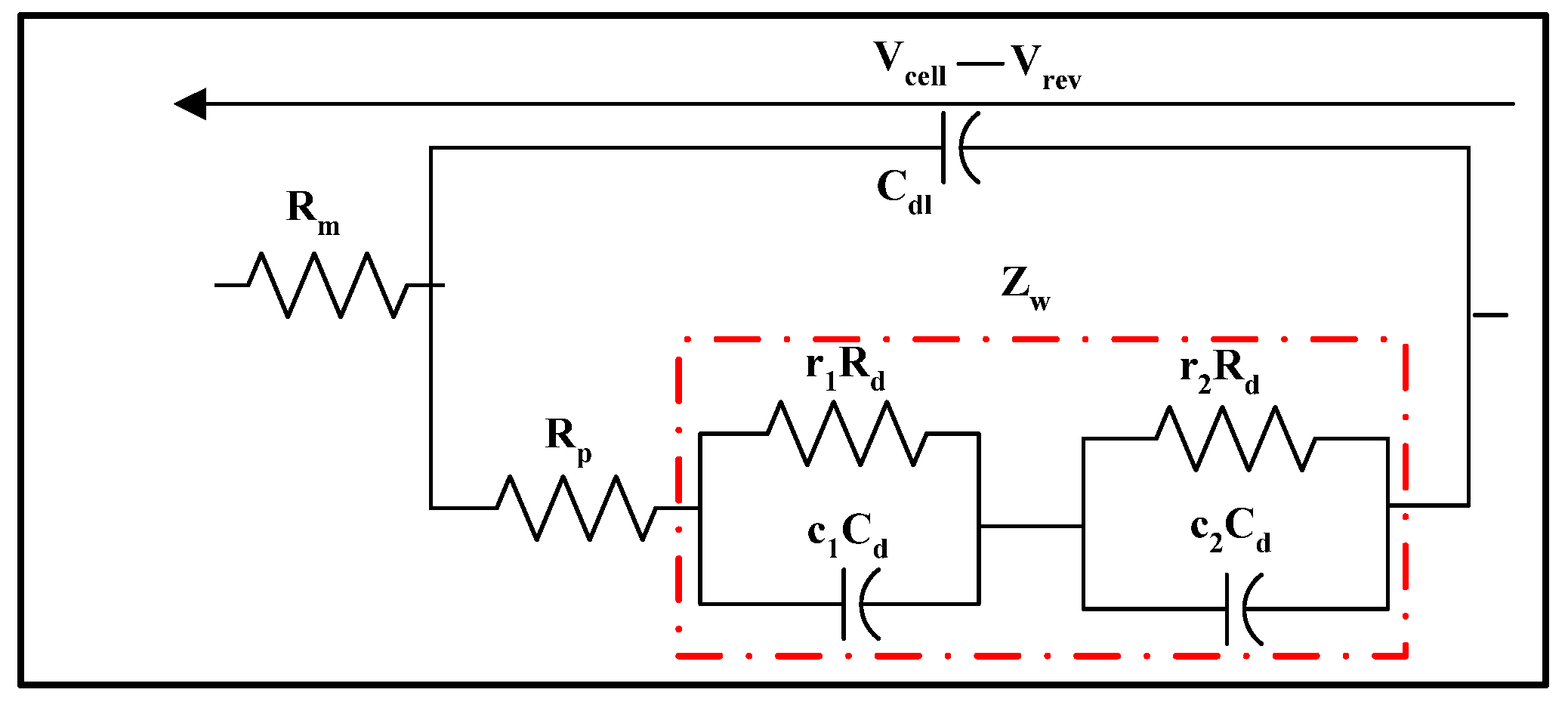
3.3.6. Warburg and Randles Circuits
- The membrane resistance, which accounts for the ohmic losses;
- The charge transfer resistance, which reflects the activation losses;
- The double layer capacitance, which represents the capacitance created by the applied electric field across the collector plates of the electrolyser;
- The Warburg impedance, which accounts for the concentration losses.
- is the diffusion resistance ];
- is the diffusion capacitor [F];
- is the diffusion time constant [s];
- is the Warburg impedance ];
- The coefficients , , , and were estimated by parameter fitting and were computed by means of a Levenberg–Marquardt algorithm.
3.3.7. Simple Equivalent Electrical Model
4. Discussion
5. Conclusions
Author Contributions
Funding
Data Availability Statement
Conflicts of Interest
Parameters
| change in the reaction enthalpy for this endothermic reaction [] | the conductor cross-sectional area [] | ||
| Stoichiometric factor for product and reactant. | Ionic resistance [] | ||
| The stoichiometric factors are: [] | : | is the thickness of the membrane [cm] | |
| enthalpies of formation of the products [] | : | is the conductivity of the membrane [] | |
| enthalpies of formation of the reactants [] | : | is the hydration rate [-] | |
| Change in Gibbs Free Energy or Free enthalpy of reaction [] | diffusion coefficient of the species X or Y | ||
| T: | Temperature of the cell [] | : | The diffusion limit current [A] |
| : | Molar change in Entropy [] | The diffusion limit current density [] | |
| Anode reversible voltage [V] | Concentration in the channel [] | ||
| : | Cathode reversible voltage [V] | Diffusion length of zone A and B. [m] | |
| : | Cell voltage [V] | , | are the diffusion limit currents [A] effective respectively in zones A and B. |
| Reversible voltage (V) | β: | coefficient considering the contribution of all diffusion overvoltage [-]. This parameter will be identified experimentally. | |
| : | Anode activation over voltage [] | [-] | |
| Cathode activation overvoltage [] | P: | Pressure [bar] | |
| : | Ohmic overvoltage [V] | : | Molar flow of hydrogen [] |
| : | Diffusion Overvoltage [] | Current efficiency [-] | |
| F: | Faraday’s constant [] | A: | Cell area [] |
| Reversible voltage at standard condition [V] | Empiric coefficients | ||
| : | Universal gas constant [8.314 ] | The capacitive current of the electrochemical double layer [A] | |
| : | Hydrogen pressure [bar] | : | the double layer capacitance [F] |
| : | Oxygen pressure [bar] | electrical permittivity [] | |
| : | References Pressure [bar] | : | Active surface of electrode |
| n: | the number of moving electrons in the chemical reaction | d: | is the distance between the electrode and the electrolyte [m]. |
| [n = 2] | : | Electrode current [A] | |
| Gibbs Free Energy at standard condition [] | The faradic current (current linked to activation phenomena) [A] | ||
| Cell current density [] | Diffusion resistance | ||
| Exchange current density at electrodes [] | Capacitor of the diffusion phenomena [F] | ||
| The concentrations of the reaction product and reactant in the vicinity of the electrode [] | : | The diffusion curent [A] | |
| The concentration of the reaction product and reactant in the solution [] | Diffusion resistance ] | ||
| Charge transfer coefficient [-] | Diffusion time constant [s] | ||
| Activation overvoltage at both electrodes [V] | Warburg impedance ] | ||
| k: | refer to anode, cathode [-] | and : | are the capacitors for anode and cathode (F) |
| the leakage current density due to crossover [] | and : | are the resistances for anode and cathode (F) | |
| : | is the global transfer coefficient [] | and | Time constant (s) |
| is the total activation overvoltage [] | Molar flow of species [] | ||
| Anode charge transfer coefficient [-] | Concentration of species X or Y in and at time t | ||
| Cathode charge transfer coefficient [-] | is the coordinate [m] on the axis [) | ||
| Cell current [] | Time [s] | ||
| A: | is the surface of the cell [] | ||
| : | The membrane overvoltage [V] | ||
| The electronic overvoltage [V] | |||
| Electronic resistance [] | |||
| L: | the length of the path of the electrons [cm] | ||
| : | electrode material resistivity [m] | ||
Appendix A
Appendix A.1. Description of Convective Diffusion Phenomenon

- One where the species is produced and evacuated from the electrolyser ( and );
- One where the species is brought in and consumed within the electrolyser ( for the latter case).

- molar flow of species X or Y [mol/s];
- concentration of species X or Y in and at time t ;
- the coordinate [m] on the axis [);
- time [s].
Appendix A.2. First Case: Species Produced and Evacuated from the Component ( and )
Appendix A.3. Second Case: Species Introduced and Consumed within the Component (O)
- One where the species is produced and evacuated from the component ( and );
- Another where the species is introduced and consumed within the component ().
Appendix B
Appendix B.1. Calculation of Diffusion Impedance
- E (0, t): electrode potential [V];
- [Ox] (0, t): concentration of oxidizing species [];
- [Red] (0, t): concentration of reducing species [].
- the charge transfer or activation resistance [];
- ZOx(p): the concentration or diffusion impedance of the oxidizing species [].
- ZRed(p): the concentration or diffusion impedance of the reducing species [].
- Potential of electrode [V];
- rate constant of oxidation and reduction;
- transfer coefficient (), which indicate in which direction the reaction is favored. If > 0.5, the reaction in the direction of oxidation (anodic direction) is favored; if > 0.5, the reaction in the reduction direction (cathode direction) is favoured.
- diffusion coefficient [].
- diffusion flow in the direction of oxidation [];
- diffusion flow in the direction of reduction [].
Appendix C
| Ref. | Membrane Thickness | Charge Transfer (-) | ) | Membrane Surface Area | ||||
|---|---|---|---|---|---|---|---|---|
| Nafion 115 | Nafion 117 | etc. | Anode | Cathode | Anode | Cathode | ||
| [19] | 178 | 0.5 | 0.5 | Pt: Pt-Ir: | Pt: | |||
| [68] | 0.05–0.2 mm | 0.5 | 0.5 | 0.01–10 | 160 | |||
| [29] | 0.7178 | 0.6395 | ||||||
| [41] | 0.18–0.42 | |||||||
| [69] | 178 | 0.18–0.42 | 0.5 | |||||
| [27] | 178 | 0.1–0.6 | 0.5 | 86.4 (20 cells) | ||||
| [31] | Nafion 110 | 0.5 | 0.5 | Pt: Pt-Ir: | 160 | |||
| [36] | 100 | 0.5 | 0.5 | 1 | ||||
| [28] | Nafion 112 | 0.5 | 0.5 | 50 of active area-2 cells | ||||
| [47] | 178 | 0.5 | 0.5 | 5 | ||||
| [21] | 0.0254 cm | 0.8 | 0.25 | 160 | ||||
| [70] | 200 | Electrode surface area 1 cm2 | ||||||
- Literature values for i0 are also greatly dispersed in a range between ;
- In practice, the thickness of the electrolyte membrane of a PEM electrolyser can range from 50 to 200 .
References
- AR5 Climate Change 2013: The Physical Science Basis—IPCC. Available online: https://www.ipcc.ch/report/ar5/wg1/ (accessed on 13 March 2023).
- Liu, Y.; Jiang, S.P.; Shao, Z. Intercalation pseudocapacitance in electrochemical energy storage: Recent advances in fundamental understanding and materials development. Mater. Today Adv. 2020, 7, 100072. [Google Scholar] [CrossRef]
- Sood, S. Multiphysics Modelling for Online Diagnosis and Efficiency Tracking: Application to Green H2 Production. Ph.D. Thesis, Université de Lille, Lille, France, 2021. Available online: https://theses.hal.science/tel-03675228 (accessed on 17 June 2023).
- Veziro, T.N.; Barbir, F. Hydrogen: The wonder fuel. Int. J. Hydrogen Energy 1992, 17, 391–404. [Google Scholar] [CrossRef]
- Yilanci, A.; Dincer, I.; Ozturk, H.K. A review on solar-hydrogen/fuel cell hybrid energy systems for stationary applications. Prog. Energy Combust. Sci. 2009, 35, 231–244. [Google Scholar] [CrossRef]
- Singh, S.; Jain, S.; Venkateswaran, P.S.; Tiwari, A.K.; Nouni, M.R.; Pandey, J.K.; Goel, S. Hydrogen: A sustainable fuel for future of the transport sector. Renew. Sustain. Energy Rev. 2015, 51, 623–633. [Google Scholar] [CrossRef]
- Gahleitner, G. Hydrogen from renewable electricity: An international review of power-to-gas pilot plants for stationary applications. Int. J. Hydrogen Energy 2013, 38, 2039–2061. [Google Scholar] [CrossRef]
- Albadi, M.H.; El-Saadany, E.F. Overview of wind power intermittency impacts on power systems. Electr. Power Syst. Res. 2010, 80, 627–632. [Google Scholar] [CrossRef]
- Zhang, G.; Wan, X. A wind-hydrogen energy storage system model for massive wind energy curtailment. Int. J. Hydrogen Energy 2014, 39, 1243–1252. [Google Scholar] [CrossRef]
- Nitsch, J.; Klaiss, H.; Meyer, J. The contribution of hydrogen in the development of renewable energy sources. Int. J. Hydrogen Energy 1992, 17, 651–663. [Google Scholar] [CrossRef]
- Hernández-Gómez, Á.; Ramirez, V.; Guilbert, D. Investigation of PEM electrolyzer modeling: Electrical domain, efficiency, and specific energy consumption. Int. J. Hydrogen Energy 2020, 45, 14625–14639. [Google Scholar] [CrossRef]
- Falcão, D.S.; Pinto, A.M.F.R. A review on PEM electrolyzer modelling: Guidelines for beginners. J. Clean. Prod. 2020, 261, 121184. [Google Scholar] [CrossRef]
- Olivier, P.; Bourasseau, C.; Bouamama, P.B. Low-temperature electrolysis system modelling: A review. Renew. Sustain. Energy Rev. 2017, 78, 280–300. [Google Scholar] [CrossRef]
- Bessarabov, D.G.; Wang, H.H.; Li, H.; Zhao, N. (Eds.) PEM Electrolysis for Hydrogen Production: Principles and Applications; CRC Press: Boca Raton, FL, USA; London, UK, 2016. [Google Scholar]
- Rozain, C. Développement de Nouveaux Matériaux d’Electrodes pour la Production d’Hydrogène par Electrolyse de l’eau. Ph.D. Thesis, Université Paris Sud-Paris XI, Bures-sur-Yvette, France, 2013. Available online: https://theses.hal.science/tel-00923169 (accessed on 13 March 2023).
- Kauranen, P.S.; Lund, P.D.; Vanhanen, J.P. Development of a self-sufficient solar-hydrogen energy system. Int. J. Hydrogen Energy 1994, 19, 99–106. [Google Scholar] [CrossRef]
- Görgün, H. Dynamic modelling of a proton exchange membrane (PEM) electrolyzer. Int. J. Hydrogen Energy 2006, 31, 29–38. [Google Scholar] [CrossRef]
- Shen, M.; Bennett, N.; Ding, Y.; Scott, K. A concise model for evaluating water electrolysis. Int. J. Hydrogen Energy 2011, 36, 14335–14341. [Google Scholar] [CrossRef]
- Choi, P.; Bessarabov, D.G.; Datta, R. A simple model for solid polymer electrolyte (SPE) water electrolysis. Solid State Ion. 2004, 175, 535–539. [Google Scholar] [CrossRef]
- Zhang, H.; Su, S.; Lin, G.; Chen, J. Efficiency Calculation and Configuration Design of a PEM Electrolyzer System for Hydrogen Production. Int. J. Electrochem. Sci. 2012, 7, 4143–4157. [Google Scholar] [CrossRef]
- Abdin, Z.; Webb, C.J.; Gray, E.M. Modelling and simulation of a proton exchange membrane (PEM) electrolyser cell. Int. J. Hydrogen Energy 2015, 40, 13243–13257. [Google Scholar] [CrossRef]
- Kang, Z.; Alia, S.M.; Young, J.L.; Bender, G. Effects of various parameters of different porous transport layers in proton exchange membrane water electrolysis. Electrochim. Acta 2020, 354, 136641. [Google Scholar] [CrossRef]
- Lefranc, O. Développement d’un outil de Conception de Micro-Réseaux Energétiques”. Ph.D. Thesis, Toulouse, INPT, Toulouse, France, 2021. Available online: https://theses.hal.science/tel-04186359 (accessed on 17 June 2023).
- Hammoudi, M.; Henao, C.; Agbossou, K.; Dubé, Y.; Doumbia, M.L. New multi-physics approach for modelling and design of alkaline electrolyzers. Int. J. Hydrogen Energy 2012, 37, 13895–13913. [Google Scholar] [CrossRef]
- Henao, C.; Agbossou, K.; Hammoudi, M.; Dubé, Y.; Cardenas, A. Simulation tool based on a physics model and an electrical analogy for an alkaline electrolyser. J. Power Sources 2014, 250, 58–67. [Google Scholar] [CrossRef]
- da Costa Lopes, F.; Watanabe, E.H. Experimental and theoretical development of a PEM electrolyzer model applied to energy storage systems. In Proceedings of the 2009 Brazilian Power Electronics Conference, Bonito-Mato Grosso do Sul, Brazil, 27 September–1 October 2009; pp. 775–782. [Google Scholar] [CrossRef]
- Dale, N.V.; Mann, M.D.; Salehfar, H. Semiempirical model based on thermodynamic principles for determining 6 kW proton exchange membrane electrolyzer stack characteristics. J. Power Sources 2008, 185, 1348–1353. [Google Scholar] [CrossRef]
- García-Valverde, R.; Espinosa, N.; Urbina, A. Simple PEM water electrolyser model and experimental validation. Int. J. Hydrogen Energy 2012, 37, 1927–1938. [Google Scholar] [CrossRef]
- Agbli, K.S.; Péra, M.C.; Hissel, D.; Rallières, O.; Turpin, C.; Doumbia, I. Multiphysics simulation of a PEM electrolyser: Energetic Macroscopic Representation approach. Int. J. Hydrogen Energy 2011, 36, 1382–1398. [Google Scholar] [CrossRef]
- Ursúa, A.; Sanchis, P. Static–dynamic modelling of the electrical behaviour of a commercial advanced alkaline water electrolyser. Int. J. Hydrogen Energy 2012, 37, 18598–18614. [Google Scholar] [CrossRef]
- Marangio, F.; Santarelli, M.; Calì, M. Theoretical model and experimental analysis of a high pressure PEM water electrolyser for hydrogen production. Int. J. Hydrogen Energy 2009, 34, 1143–1158. [Google Scholar] [CrossRef]
- Roy, A.; Watson, S.; Infield, D. Comparison of electrical energy efficiency of atmospheric and high-pressure electrolysers. Int. J. Hydrogen Energy 2006, 31, 1964–1979. [Google Scholar] [CrossRef]
- Rallières, O. Modélisation et Caractérisation de Piles a Combustible et Electrolyseurs PEM. Ph.D. Thesis, Toulouse, INPT, Toulouse, France, 2011. Available online: https://www.theses.fr/2011INPT0128 (accessed on 13 March 2023).
- Rabih, S. Contribution à la Modélisation de Systèmes Réversibles de Types Electrolyseur et Pile à Hydrogène en vue de leur Couplage aux Générateurs Photovoltaïques. Ph.D. Thesis, Toulouse, INPT, Toulouse, France, 2008. Available online: http://ethesis.inp-toulouse.fr/archive/00000677/ (accessed on 13 March 2023).
- Igourzal, A.; Auger, F.; Olivier, J.-C.; Retière, C. Electrical and thermal modelling of PEMFCs for naval applications. Math. Comput. Simul. 2023, 206, S0378475423001817. [Google Scholar] [CrossRef]
- Ni, M.; Leung, M.K.H.; Leung, D.Y.C. Energy and exergy analysis of hydrogen production by a proton exchange membrane (PEM) electrolyzer plant. Energy Convers. Manag. 2008, 49, 2748–2756. [Google Scholar] [CrossRef]
- Sawada, S.; Yamaki, T.; Maeno, T.; Asano, M.; Suzuki, A.; Terai, T.; Maekawa, Y. Solid polymer electrolyte water electrolysis systems for hydrogen production based on our newly developed membranes, Part I: Analysis of voltage–current characteristics. Prog. Nucl. Energy 2008, 50, 443–448. [Google Scholar] [CrossRef]
- Grigoriev, S.A.; Kalinnikov, A.A.; Millet, P.; Porembsky, V.I.; Fateev, V.N. Mathematical modeling of high-pressure PEM water electrolysis. J. Appl.Electrochem. 2010, 40, 921–932. [Google Scholar] [CrossRef]
- Lee, B.; Park, K.; Kim, H.-M. Dynamic Simulation of PEM Water Electrolysis and Comparison with Experiments. Int. J. Electrochem. Sci. 2013, 8, 235–248. [Google Scholar] [CrossRef]
- Lebbal, M.E.; Lecœuche, S. Identification and monitoring of a PEM electrolyser based on dynamical modelling. Int. J. Hydrogen Energy 2009, 34, 5992–5999. [Google Scholar] [CrossRef]
- Awasthi, A.; Scott, K.; Basu, S. Dynamic modeling and simulation of a proton exchange membrane electrolyzer for hydrogen production. Int. J. Hydrogen Energy 2011, 36, 14779–14786. [Google Scholar] [CrossRef]
- Kim, H.; Park, M.; Lee, K.S. One-dimensional dynamic modeling of a high-pressure water electrolysis system for hydrogen production. Int. J. Hydrogen Energy 2013, 38, 2596–2609. [Google Scholar] [CrossRef]
- Ulleberg, Ø. Modeling of advanced alkaline electrolyzers: A system simulation approach. Int. J. Hydrogen Energy 2003, 28, 21–33. [Google Scholar] [CrossRef]
- Fontes, G. Modélisation et Caractérisation de la pile PEM pour l’étude des Interactions Avec les Convertisseurs Statiques. Ph.D. Thesis, Toulouse, INPT, Toulouse, France, 2005. Available online: https://www.theses.fr/2005INPT020H (accessed on 13 March 2023).
- Springer, T.E.; Zawodzinski, T.A.; Gottesfeld, S. Polymer Electrolyte Fuel Cell Model. J. Electrochem. Soc. 1991, 138, 2334. [Google Scholar] [CrossRef]
- Brown, T.M.; Brouwer, J.; Samuelsen, G.S.; Holcomb, F.H.; King, J. Dynamic first principles model of a complete reversible fuel cell system. J. Power Sources 2008, 182, 240–253. [Google Scholar] [CrossRef]
- Han, B.; Steen, S.M.; Mo, J.; Zhang, F.-Y. Electrochemical performance modeling of a proton exchange membrane electrolyzer cell for hydrogen energy. Int. J. Hydrogen Energy 2015, 40, 7006–7016. [Google Scholar] [CrossRef]
- Maruf-ul-Karim, M.; Iqbal, M.T. Dynamic modeling and simulation of alkaline type electrolyzers. In Proceedings of the 2009 Canadian Conference on Electrical and Computer Engineering, St. John’s, NL, Canada, 3–6 May 2009; pp. 711–715. [Google Scholar] [CrossRef]
- Sánchez, M.; Amores, E.; Rodríguez, L.; Clemente-Jul, C. Semi-empirical model and experimental validation for the performance evaluation of a 15 kW alkaline water electrolyzer. Int. J. Hydrogen Energy 2018, 43, 20332–20345. [Google Scholar] [CrossRef]
- Hug, W.; Bussmann, H.; Brinner, A. Intermittent operation and operation modeling of an alkaline electrolyzer. Int. J. Hydrogen Energy 1993, 18, 973–977. [Google Scholar] [CrossRef]
- Baurens, P.; Serre-Combe, P.; Poirot-Crouvezier, J.-P. Fuel Cells. In Low Emission Power Generation Technologies and Energy Management; John Wiley & Sons, Ltd.: Hoboken, NJ, USA, 2013; pp. 179–262. [Google Scholar] [CrossRef]
- Barbir, F. PEM electrolysis for production of hydrogen from renewable energy sources. Sol. Energy 2005, 78, 661–669. [Google Scholar] [CrossRef]
- Artuso, P.; Gammon, R.; Orecchini, F.; Watson, S.J. Alkaline electrolysers: Model and real data analysis. Int. J. Hydrogen Energy 2011, 36, 7956–7962. [Google Scholar] [CrossRef]
- Atlam, O.; Kolhe, M. Equivalent electrical model for a proton exchange membrane (PEM) electrolyser. Energy Convers. Manag. 2011, 52, 2952–2957. [Google Scholar] [CrossRef]
- Martinson, C.; van Schoor, G.; Uren, K.; Bessarabov, D. Equivalent electrical circuit modelling of a Proton Exchange Membrane electrolyser based on current interruption. In Proceedings of the 2013 IEEE International Conference on Industrial Technology (ICIT), Cape Town, South Africa, 25–28 February 2013; pp. 716–721. [Google Scholar] [CrossRef]
- Rozain, C.; Millet, P. Electrochemical characterization of Polymer Electrolyte Membrane Water Electrolysis Cells. Electrochim. Acta 2014, 131, 160–167. [Google Scholar] [CrossRef]
- Martinson, C.A.; van Schoor, G.; Uren, K.R.; Bessarabov, D. Characterisation of a PEM electrolyser using the current interrupt method. Int. J. Hydrogen Energy 2014, 39, 20865–20878. [Google Scholar] [CrossRef]
- Guilbert, D.; Vitale, G. Experimental Validation of an Equivalent Dynamic Electrical Model for a Proton Exchange Membrane Electrolyzer. In Proceedings of the 2018 IEEE International Conference on Environment and Electrical Engineering and 2018 IEEE Industrial and Commercial Power Systems Europe (EEEIC/I&CPS Europe), Palermo, Italy, 12–15 June 2018; pp. 1–6. [Google Scholar] [CrossRef]
- Hernández-Gómez, Á.; Ramirez, V.; Guilbert, D.; Saldivar, B. Development of an adaptive static-dynamic electrical model based on input electrical energy for PEM water electrolysis. Int. J. Hydrogen Energy 2020, 45, 18817–18830. [Google Scholar] [CrossRef]
- Macdonald, J.R.; Johnson, W.B. Fundamentals of Impedance Spectroscopy. In Impedance Spectroscopy; John Wiley & Sons, Ltd.: Hoboken, NJ, USA, 2005; pp. 1–26. [Google Scholar] [CrossRef]
- Serna, Á.; Yahyaoui, I.; Normey-Rico, J.E.; De Prada, C.; Tadeo, F. Predictive control for hydrogen production by electrolysis in an offshore platform using renewable energies. Int. J. Hydrogen Energy 2017, 42, 12865–12876. [Google Scholar] [CrossRef]
- Abdelghany, M.B.; Shehzad, M.F.; Liuzza, D.; Mariani, V.; Glielmo, L. Optimal operations for hydrogen-based energy storage systems in wind farms via model predictive control. Int. J. Hydrogen Energy 2021, 46, 29297–29313. [Google Scholar] [CrossRef]
- Nasser, M.; Megahed, T.F.; Ookawara, S.; Hassan, H. A review of water electrolysis–based systems for hydrogen production using hybrid/solar/wind energy systems. Environ. Sci. Pollut. Res. 2022, 29, 86994–87018. [Google Scholar] [CrossRef]
- Wang, H.; Sun, M.; Ren, J.; Yuan, Z. Circumventing Challenges: Design of Anodic Electrocatalysts for Hybrid Water Electrolysis Systems. Adv. Energy Mater. 2023, 13, 2203568. [Google Scholar] [CrossRef]
- Zhou, T.; Francois, B. Modeling and control design of hydrogen production process for an active hydrogen/wind hybrid power system. Int. J. Hydrogen Energy 2009, 34, 21–30. [Google Scholar] [CrossRef]
- Nafchi, F.M.; Baniasadi, E.; Afshari, E.; Javani, N. Performance assessment of a solar hydrogen and electricity production plant using high temperature PEM electrolyzer and energy storage. Int. J. Hydrogen Energy 2018, 43, 5820–5831. [Google Scholar] [CrossRef]
- Wind-to-Hydrogen Tech Goes to Sea-IEEE Spectrum. Available online: https://spectrum.ieee.org/green-hydrogen-2663997448 (accessed on 26 August 2023).
- Toghyani, S. Optimization of operating parameters of a polymer exchange membrane electrolyzer. Int. J. Hydrogen Energy 2019, 44, 6403–6414. [Google Scholar] [CrossRef]
- Biaku, C.; Dale, N.; Mann, M.; Salehfar, H.; Peters, A.; Han, T. A semiempirical study of the temperature dependence of the anode charge transfer coefficient of a 6kW PEM electrolyzer. Int. J. Hydrogen Energy 2008, 33, 4247–4254. [Google Scholar] [CrossRef]
- Ahn, J.; Holze, R. Bifunctional electrodes for an integrated water-electrolysis and hydrogen-oxygen fuel cell with a solid polymer electrolyte. J. Appl. Electrochem. 1992, 22, 1167–1174. [Google Scholar] [CrossRef]


| Voltages | Section | Equation Numbers |
|---|---|---|
| Reversible Overvoltage () | Reversible Voltage | (7)–(13) |
| Activation Overvoltage () | Activation Overvoltage | (20)–(26) |
| Ohmic Overvoltage () | Ohmic Overvoltage | (30)–(34) |
| Diffusion Overvoltage () | Diffusion Overvoltage | (43)–(45) |
Disclaimer/Publisher’s Note: The statements, opinions and data contained in all publications are solely those of the individual author(s) and contributor(s) and not of MDPI and/or the editor(s). MDPI and/or the editor(s) disclaim responsibility for any injury to people or property resulting from any ideas, methods, instructions or products referred to in the content. |
© 2023 by the authors. Licensee MDPI, Basel, Switzerland. This article is an open access article distributed under the terms and conditions of the Creative Commons Attribution (CC BY) license (https://creativecommons.org/licenses/by/4.0/).
Share and Cite
Marefatjouikilevaee, H.; Auger, F.; Olivier, J.-C. Static and Dynamic Electrical Models of Proton Exchange Membrane Electrolysers: A Comprehensive Review. Energies 2023, 16, 6503. https://doi.org/10.3390/en16186503
Marefatjouikilevaee H, Auger F, Olivier J-C. Static and Dynamic Electrical Models of Proton Exchange Membrane Electrolysers: A Comprehensive Review. Energies. 2023; 16(18):6503. https://doi.org/10.3390/en16186503
Chicago/Turabian StyleMarefatjouikilevaee, Haniyeh, Francois Auger, and Jean-Christophe Olivier. 2023. "Static and Dynamic Electrical Models of Proton Exchange Membrane Electrolysers: A Comprehensive Review" Energies 16, no. 18: 6503. https://doi.org/10.3390/en16186503
APA StyleMarefatjouikilevaee, H., Auger, F., & Olivier, J.-C. (2023). Static and Dynamic Electrical Models of Proton Exchange Membrane Electrolysers: A Comprehensive Review. Energies, 16(18), 6503. https://doi.org/10.3390/en16186503