Abstract
As autonomous vehicle technology advances, the development of energy-efficient control methodologies emerges as a critical area in the literature. This includes the behavior control of vehicles near signalized intersections, which still needs comprehensive exploration. Through connectivity, the adoption of promising eco-driving approaches can manage a vehicle’s speed profile to improve energy consumption. This study focuses on controlling the speed of an autonomous electric vehicle (AEV) both up and downstream of a signalized intersection in the presence of preceding vehicles. In order to achieve this, a dynamic pro-active predictive cruise control eco-driving (eco-PPCC) framework is developed that, instead of merely reacting to the preceding vehicle’s speed changes, uses the preceding vehicle’s upcoming data to actively adjust and optimize the speed profile of the AEV. The proposed algorithm is compared to the conventional Gipps and eco-PCC models for benchmarking and performance analysis through numerous scenarios. Additionally, real-world measurements are performed and taken to consider practical use cases. The results demonstrate that when compared to the two baseline methods, the proposed framework can add significant value to reducing energy consumption, preventing unnecessary stops at intersections, and improving travel time.
1. Introduction
The transportation industry in the United States accounts for 28% of total energy consumption and 26% of greenhouse gas (GHG) emissions [1]. In urban areas, approximately 25% of these emissions stem from traffic stops [2]. One way to reduce energy consumption and emissions is ecological driving (eco-driving). Eco-driving utilizes strategies such as optimal velocity/acceleration planning and gear shifting to improve energy efficiency. The emergence of intelligent transportation systems (ITSs) has brought about the creation of connected vehicles (CVs) and connected automated vehicles (CAVs), which utilize vehicle-to-vehicle (V2V) and vehicle-to-infrastructure (V2I) communications to improve energy efficiency, reduce GHG emissions, and enhance driving safety and comfort. By combining eco-driving with these recent advancements in connectivity, one can consider important factors like signal phase and timing (SPaT) and traffic flow conditions to provide optimal real-time commands to the vehicle, optimizing its performance [3].
1.1. Literature Review
In general, research related to driver assistance systems, speed advisory systems, velocity planning, and eco-driving can be divided into highway and urban road strategies. In the area of eco-driving on highways, Han et al. developed an eco-driving system that minimizes energy consumption using an optimal control problem (OCP) formulation for a case study on highway roads [4]. In mixed highway-urban traffic, a real-time dynamic predictive cruise control (PCC) system was developed based on a bi-level model predictive control (MPC) algorithm using SPaT information to pass the nearest signal intersection during the green light interval without stopping, reducing energy consumption levels by 8.5–15.6% compared to the Intelligent driver model (IDM) [3].
Although eco-driving on highways is important, eco-driving in urban areas presents more difficulties due to the complex constraints imposed by SPaT on the eco-driving problem. Since this paper focuses on eco-driving in urban areas, the following section delves deeper into existing studies on urban eco-driving. There are three main types of urban eco-driving: eco-driving with a focus on road conditions, eco-driving that considers traffic signal limitations, and eco-driving that considers the behavior of the preceding vehicle.
In the first research field, dynamic programming (DP) is used to optimize fuel consumption on hilly terrains with various road grades, achieving a 7–30% fuel economy improvement [5]. In [6], a control algorithm was introduced to optimize the velocity profile and gear shifting for fuel efficiency using a DP approach, considering the road’s topography. Additionally, Weißmann et al. developed a system that combines adaptive cruise control (ACC) with MPC and DP to determine the most energy-efficient speed trajectory, taking into consideration factors like road slope and speed limitations [7].
Considerable research efforts have been dedicated to studying eco-driving near signalized intersections. It includes investigations into utilizing forthcoming traffic signal details within ACC systems to minimize the idle time spent waiting behind traffic lights, as explored in [8]. Furthermore, the utilization of SPaT information to decrease the frequency of stopping at traffic lights for a group of CVs through V2V communication has been examined, as highlighted in [9]. A bi-level eco-driving optimization for connected fuel cell hybrid electric vehicles (FCHEVs), including speed planning as the upper level and energy management as the lower level, is also developed, considering traffic light constraints during a corridor of multiple intersections [10]. Although eco-driving techniques are mainly designed for the upstream of the intersection, as indicated in [11,12], there is a scarcity of research focused on eco-driving strategies for the downstream of signalized intersections, namely the departure phase after the traffic lights [13]. The best solutions for optimizing traffic flow at a signalized intersection may differ depending on whether only the upstream of the intersection is considered or if both upstream and downstream are taken into account. In cases where a vehicle needs to slow down before reaching the traffic light, a strategy focused solely on the upstream of the intersection may recommend coming to a complete stop, as this recuperates more energy through braking. However, this results in energy loss when the vehicle accelerates back downstream of the intersection. The joint optimization of both upstream and downstream can prevent this energy loss. Therefore, from a holistic point of view, eco-approach-and-departure systems [1,14] offer the potential to enhance the effectiveness of eco-driving strategies.
The third type of eco-driving, car-following-based eco-driving, is frequently integrated with the first two categories. In line with this, a study in [15] investigates an eco-driving system designed for CAVs approaching a traffic signal. The system considers both the timing of the traffic signal and the behavior of the preceding vehicle to optimize fuel efficiency. Moreover, in [16], a PCC eco-driving system is proposed. The system utilizes an MPC framework and dynamically switches between three strategies: free driving, anticipation of signal timing, and car following. The three-level PCC system yields energy consumption reductions ranging from 12.5% to 30.3%, depending on the specific traffic conditions.
Previous research has focused on reducing energy consumption or GHG emissions through velocity planning and eco-driving strategies. Some studies have indirectly aimed to enhance energy efficiency. For example, a driving system that avoids sudden braking is developed in [17]. Moreover, a multi-objective optimization problem that strives to enhance speed profile smoothness while simultaneously minimizing travel time is suggested in [2]. Another study introduced a predictive optimal velocity planning algorithm to increase the probability of crossing intersections during green light intervals [18].
Several previous studies have directly considered energy consumption as their objective function. In [19], a time-dependent optimal speed profile was proposed to minimize the electricity consumption of an electric vehicle (EV). In another study, a speed guidance strategy combined with a car-following model is developed to optimize fuel consumption [20]. Moreover, fuel-optimized vehicle trajectory using SPaT information was introduced in [21] for CAVs. Some studies have attempted to define multiple objectives alongside energy consumption, such as minimizing the speed difference, travel time, and energy consumption for a platoon of CVs [22]. A study on a bi-level eco-driving control strategy for connected and automated hybrid electric vehicles (CAHEVs) to optimize safety, energy consumption, and GHG emissions is presented in [23]. The latest research works endeavor to optimize both energy usage and travel time at the same time. A speed plan for CAVs was developed in [24] to optimize fuel consumption and travel time.
In order to achieve energy-efficient eco-driving, employing a precise model for estimating energy consumption is vital. Since eco-driving for internal combustion engine (ICE) vehicles has been extensively studied in the literature, most of the available models for energy consumption estimation are focused on fuel consumption. In [25], the fuel consumption rate model introduced in [26] is employed that estimates fuel usage based on driving inputs. Xiang et al. employed a quasi-static engine model based on power and used the vehicle dynamics and model parameters obtained through the curve fitting of mapped engine data [27]. In [28], a statistical fuel consumption model is applied that utilizes a piecewise instantaneous fuel consumption model based on vehicle-specific power (VSP). In [29], a fuel consumption rate estimation model for flat roads was developed based on statistical data, which is also used by Wan et al. in [30]. The Virginia Tech Comprehensive Power-based Fuel Consumption Model (VT-CPFM) is a widely recognized microscopic model that has been utilized in multiple studies, including [21,31].
A limited number of studies in the existing literature report the development of energy consumption models specifically for EVs and autonomous vehicles (AVs). In [32], an energy consumption estimation for a parallel hybrid electric vehicle (PHEV) that considers the torque and speed of the engine and motor was conducted. Other research studies, such as [33,34], utilized vehicle dynamics to calculate the instantaneous power at the wheels to estimate energy consumption.
Furthermore, in [35], the aim was to minimize the forces during driving and braking, as well as the inverse of the velocity, which represents time. Assuming a constant traveled distance, the objective functions presented in [35] are equivalent to minimizing energy consumption and travel time. However, that particular study did not consider the efficiency aspect of regenerative braking, which holds significance in the powertrains of today’s EVs and hybrid electric vehicles (HEVs). Moreover, many other studies have not accounted for auxiliary energy consumption.
Most research in this field has focused on eco-driving strategies for vehicles approaching traffic lights to minimize the number of stops at red lights, reduce energy consumption, lower GHG emissions, or achieve a combination of these objectives. However, many of these studies have solely considered the influence of SPaT information. Only a few studies have considered both SPaT-related information and the behavior of vehicles following each other. For instance, in [3,16], the reference speed is determined as the maximum feasible speed that allows the vehicle to catch the green light interval and adhere to speed limits. These studies aim to follow this reference speed while considering the constraints imposed by preceding vehicles. However, these reference speeds may not necessarily be the optimal speeds in terms of energy efficiency. Other eco-driving studies that consider both SPaT information and car-following behavior have focused on minimizing different factors. For example, in [36], the aim is to minimize greenhouse gas emissions and acceleration fluctuations. However, in [37], the consumption of auxiliary equipment is considered in a hierarchical control system based on MPC. Moreover, in [38], both regenerative braking and auxiliary energy consumption are considered. However, it was limited to the upstream of the signalized intersection. Hesami et al. [39] have covered the mentioned gaps by proposing a bi-layer eco-PCC framework in which both the up and downstream of the signalized intersection are considered.
1.2. Motivations and Contributions
Despite all the advancements in the existing studies in terms of eco-driving vehicles in the vicinity of signalized intersections, the main literature gap is that the existing models only react to the circumstances imposed by the immediate preceding vehicle (IPV). For example, in the reactive models, such as the eco-PCC framework in [39], first, the reference trajectory is optimized by considering the SPaT regardless of the IPV’s upcoming trajectory data. Then, the framework locally imposes safety considerations based on the IPV’s upcoming location data on the reference speed tracking to avoid collisions. On the contrary, a pro-active framework considers the IPV’s upcoming location in the reference trajectory optimization. It leads to a reduction in energy consumption by avoiding speed fluctuations.
This paper introduces and evaluates a robust framework designed for a pro-active eco-driving system of connected automated electric vehicles (CAEVs), which takes into account the SPaT of signalized intersections and the preceding vehicles’ upcoming trajectory data through V2V and V2I communications. The main contribution of this paper is to incorporate the IPV’s upcoming location and speed data into the reference speed planning to obtain pro-active predictive cruise control eco-driving (eco-PPCC), avoiding unnecessary speed fluctuations. Additionally, the eco-PPCC framework considers both the up and downstream sections simultaneously. Furthermore, by adding one more degree of freedom, the paper advances the analytical parameterization of energy consumption presented in the authors’ previous research work [40] by adding one more degree of freedom. The parameterized model establishes a relationship between the energy consumption and kinematic variables. Therefore, the key contributions of this research are as follows:
- Proposing a pro-active algorithm that considers the IPV state data in the reference speed planning;
- Improving existing analytical energy consumption parameterization;
- Considering both the up and downstream of the signalized intersection.
Regarding the paper’s structure, Section 2 proposes the integrated model and its analytical parameterization procedure. Section 3 focuses on the calibration and validation of the energy consumption model, along with presenting, benchmarking, and discussing the outcomes of the framework. Finally, Section 4 covers the conclusion and provides future research work directions.
2. Materials and Methods
The proposed eco-PPCC system considers the limitations imposed by the traffic lights and the preceding IPV. The problem scenario is depicted in Figure 1, assuming that the AEV is equipped with onboard sensors capable of real-time data perception to obtain the location and speed of the IPV, as well as V2V and V2I communications to obtain the upcoming IPV states and SPaT, respectively. Assuming the AEV enters the dedicated short-range communications (DSRCs) of the traffic signal’s roadside unit (RSU) at a distance of units from the traffic light, with an initial speed of , the objective is to achieve a desired speed of before it reaches a distance of units from the stop line of the traffic light. In the paper, the variables and represent the traveled distance by the AEV and the IPV, respectively. All the parameters and variables used in the paper are listed in Table 1.
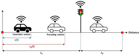
Figure 1.
The schematic of a vehicle traveling through the up and downstream of a signalized intersection in the presence of preceding vehicles.

Table 1.
List of parameters and variables.
2.1. Eco-PPCC Logic
The presented eco-PPCC framework is depicted in Figure 2. Assuming that the location information of the IPV for the next N time steps is accessible by the controlled vehicle in real-time through V2V communication, the reference planning process calculates the optimal trajectory for the remaining path, considering N future time steps. At each time step, the system evaluates the distance between the AEV and the IPV, denoted as , and compares it to the dynamic inter-vehicle safe distance, . This safe distance is determined by the relative speed between the two vehicles, as well as the time headway, and is defined as
where the variable corresponds to the minimum safe distance between the controlled vehicle and the IPV when both vehicles stand still. The speed of the controlled vehicle at time step t is indicated by , and the speed of the IPV at time step t is denoted as . Additionally, represents the duration of the safe time headway.
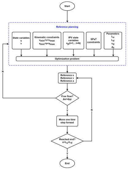
Figure 2.
Schematic of the proposed eco-PPCC framework.
If the vehicles are sufficiently distant, the controlled vehicle adheres to the calculated reference speed profile. On the other hand, if the vehicles become too close, the logic recalculates the reference trajectory using an updated N-dimensional vector of the IPV states. This iterative process continues until the controlled vehicle reaches the endpoint at .
2.2. Reference Trajectory Planning
Calculating the optimized reference trajectory involves considering several constraints, including real-time SPaT information, segment speed limits, acceleration/deceleration limits, and the minimum safe distance required between vehicles. These constraints are taken into account when formulating the problem as
Let be equal to the vehicle’s mass m, be equal to where represents air density, is the aerodynamic drag coefficient, and is the frontal area of the vehicle. is defined as , where g represents gravitational acceleration, is the friction coefficient, and is the road grade. In this study, the rolling resistance coefficient is assumed to be constant throughout the road, and the road is considered flat. equals to the auxiliary power consumption, . Additionally, denotes the drivetrain efficiency, and represents the recuperation efficiency coefficient, equal to one during acceleration and the recuperative efficiency of the vehicle during deceleration. and represent the minimum and maximum allowed speeds, while and represent the maximum deceleration and acceleration rates, respectively. In the equation, and correspond to the start and end of the green light interval. and represent the vehicle’s speed and acceleration rate at time t. and represent the initial and final times of the planned travel, respectively. denotes the time when the vehicle passes the traffic light. Variables , , and are functions of and . In Section 2.3 and Section 2.4, , , and are analytically calculated and replaced as functions of speed and acceleration. represents the location of the IPV at time t, represents the minimum safe distance between vehicles, and N represents the number of available upcoming data from the IPV. Finally,
where the regenerative braking efficiency is denoted by .
The optimization problem for eco-PPCC is formulated by considering the longitudinal dynamics of the vehicle and auxiliary energy consumption. The objective function consists of four terms considering the energy requirements at the wheels. The first three terms capture kinematic energy, aerodynamic energy losses, and energy losses due to rolling resistance and road grade. To model the energy consumption during idle mode, a time-dependent term is included in the objective function as the fourth term. This term enhances the model’s accuracy and integrates the energy model with travel time, aiming to minimize energy consumption while considering the impacts on travel time. To ensure adherence to road segment limitations and comfortable acceleration/deceleration rates, constraints are placed on the speed and acceleration of the AEV, referred to as constraints (3) and (4), respectively. Additionally, constraint (5) incorporates the SPaT information. Constraint (6) is imposed to guarantee a safe inter-vehicle distance.
Solving the optimization problem makes it possible to derive an optimal reference speed trajectory. This trajectory encompasses the optimal values for variables such as acceleration/deceleration rates and actuation timing both before and after the intersection.
2.3. Analytical Parameterization
The calculation of the definite integral in Equation (2) poses a challenge due to the involvement of unknown functions for velocity () and acceleration (), as well as the variable travel time () determined by the vehicle’s speed and acceleration. To overcome this challenge, a parameterized combination of cruising and accelerating maneuvers is devised, allowing for analytical definition and analysis. Five expected speed profile scenarios can be considered. These scenarios are
- Cruise (C): Maintaining a constant speed throughout the entire trajectory without any variations;
- Accelerate (A): Increasing or decreasing speed consistently at a fixed rate throughout the entire trajectory;
- Cruise–accelerate (C-A): Initially, cruising at a steady speed for a portion of the trajectory, followed by accelerating or decelerating at a constant rate for the remaining trajectory section;
- Accelerate–cruise (A-C): Initially, applying a constant acceleration or deceleration rate for a portion of the trajectory and maintaining a constant speed for the remaining section;
- Accelerate–cruise–accelerate (A-C-A): In the beginning, constant acceleration or deceleration occurs over a portion of the trajectory. It is followed by a phase of cruising at a constant speed. Finally, there is another phase of constant acceleration or deceleration occurs over the remaining trajectory section;
Assume that the controlled vehicle’s speed profile is a part of the speed profile shown in Figure 3. In this regard, with the assumption of and , part II shows the cruise strategy. Similarly, assuming , part III stands for the accelerate strategy, parts I-and-II show the accelerate-cruise strategy with , parts II and III show cruise-accelerate with , and the whole speed profile shows the accelerate-cruise-accelerate strategy. The fundamental reasoning behind this assumption is that speed fluctuations result in energy losses, as a portion of the kinetic energy is dissipated during braking, and a full recovery of all the kinetic energy is not feasible.
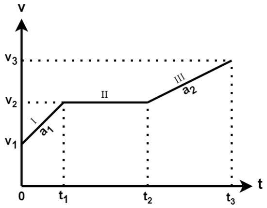
Figure 3.
Cruise and accelerate combination strategies.
During the time interval , representing the cruising stage, the speed remains constant, and the acceleration is zero. Whereas, during the time intervals and , the acceleration rate is a constant non-zero value as a, and the speed is a function of time as , where is the initial speed. The duration of each part depends on the speed and acceleration variables corresponding to that part. One can obtain , , and functions based on speed and acceleration through parameterization in each strategy. For brevity, only the algebraic operations of parameterization of the A-C-A case, as the most complex case, are presented as follows:
In part I, the time duration is
The traveled distance in parts I, II, and III are
and
respectively. By knowing that the total traveled distance is , and by substituting Equations (9)–(11) into that, after algebraic operations, we have
Based on the time duration of part III, we have
By substituting Equation (12) into Equation (13), after algebraic operations, we have
The parameterization of the other strategies can be similarly implemented. All the parameterized values are listed in Table 2.
Table 2.
Parameterized , , and for the considered five strategies.
2.4. Parameterized Objective Function
The eco-PPCC problem involves optimization while considering both a signalized intersection’s up and downstream sections. Each section is expected to have a parameterized speed profile, as illustrated in Figure 4, where represents the speed when the vehicle passes the intersection. The decision variables in the problem vary depending on the section. Specifically, in the upstream, the decision variables are , , , and , whereas, in the downstream, the decision variables are , , and . In Figure 4, variables and , which are mentioned in Equation (2), are equal to 0 and , respectively, and the variable mentioned in Equation (5) is equal to . Using Equation (16), the energy consumption of the up and downstream sections are
and
respectively. and represent the difference in elevation in the upstream and downstream sections, respectively. , , , and are the regenerative braking efficiencies of the first and second accelerated parts in the up and downstream, respectively.
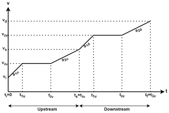
Figure 4.
Assumed speed profile in the up and downstream of the intersection.
The substitution of , , , , , and in Equations (17) and (18) yields fifth-degree polynomials. According to [41], obtaining analytical solutions for polynomial problems is considerably difficult compared to numerical solutions. Additionally, the non-convex nature of the problem, resulting from the presence of green and red timing, adds further complexity, making it challenging to find an analytical solution. Hence, this study employs a global numerical search approach instead.
2.5. Human Driver Simulation
In order to establish a benchmark, a comparison is conducted between the results of the eco-PPCC approach and those obtained from the Gipps model, which emulates human driver behavior. The Gipps model [42] provides a representation of the vehicle’s speed at time t, as
where represents the speed of the controlled vehicle at time t, denotes the maximum acceleration of the controlled vehicle, signifies the most severe deceleration rate of the controlled vehicle, indicates the most severe deceleration rate of the preceding vehicle, represents the reaction time, denotes the desired speed at time t, signifies the location of the controlled vehicle at time t, represents the location of the preceding vehicle at time t, denotes the speed of the preceding vehicle at time t, and represents the minimum safe distance between vehicles.
3. Results and Discussions
This section primarily focuses on demonstrating the calibration process. Then, the simulation results of the eco-PPCC framework performance will be presented. Finally, the eco-PPCC framework resilience in the presence of noise in the IPV data will be investigated.
3.1. Calibration
The real-world measurements obtained for this study are utilized in the calibration process. In order to conduct the calibration, a BMW i3 passenger vehicle equipped with multiple sensors was tested to accurately capture time-series data on energy consumption and vehicle location and dynamics. Detailed information about the vehicle specifications can be found on the manufacturer’s website. These specifications are included in this study. The data collection was implemented in Brussels, Belgium, at 0.64 s data resolution. Additionally, the values for the physical parameters were determined using [43]. The corresponding values for these parameters are presented in Table 3.
Table 3.
Parameter values of measurements.
The calibration process for the vehicle’s energy consumption involves utilizing real-world data. It includes adjusting the drivetrain and regenerative braking efficiency, resulting in efficiencies of and , respectively. Additionally, the calibration process determines three levels of auxiliary power consumption based on the desired cabin temperature and the environmental temperature. These levels are 970 W, 1760 W, and 2550 W for low, medium, and high levels of auxiliary power consumption, respectively. Figure 5 compares the actual power consumption of the vehicle and the power consumption predicted by theoretical calculations. This comparison demonstrates the model’s accuracy, which exhibits a normalized root mean squared error (NRMSE) of , indicating a high level of precision.
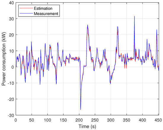
Figure 5.
Theoretical prediction and real—world measurement of energy consumption.
3.2. Eco-PPCC Framework Performance
The performance of the eco-PPCC framework is evaluated by subjecting it to analysis using the validated power consumption model. The Gipps model and the eco-PCC model presented in the authors’ previous paper [39] are chosen for benchmarking purposes. Figure 6 illustrates two case studies that assess and compare the performance of the evaluated eco-driving methods. The figure displays plots of the location and speed, with the initial and desired speeds for the preceding vehicle (IPV) ranging from km/h, which aligns with typical urban speed limits. On the x-axis of the plots, the red and green markings indicate information regarding the corresponding traffic signal phases.
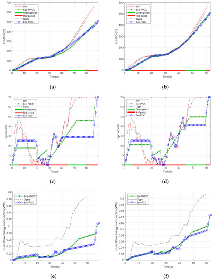
Figure 6.
Location, speed, and energy consumption of the proposed eco-PPCC framework compared to the eco-PCC and Gipps models. (a) The location, (c) speed, and (e) the cumulative energy consumption when W. (b) The location, (d) speed, and (f) the cumulative energy consumption when W.
In Figure 6a,c,e, m, which is in accordance with the normal DSRC range of the traffic light’s RSU [15,44], m, km/h, km/h, and W. Figure 6c illustrates that the proposed eco-PPCC model achieves a smooth and consistent speed profile, which is in contrast to the reactive eco-PCC model, which exhibits numerous speed fluctuations. The root mean squared variations (RMSVs) in the speed profile are km/h for eco-PCC and km/h for eco-PPCC, indicating a reduction in speed variability with the proposed model. Furthermore, Figure 6e demonstrates that the eco-PPCC model outperforms both the Gipps and eco-PCC models regarding energy efficiency. The energy consumption values are kWh for Gipps, kWh for eco-PCC, and kWh for eco-PPCC. It indicates energy savings of and compared to Gipps and eco-PCC, respectively. In addition, it is essential to reduce the impact on travel time while optimizing energy. In this regard, the proposed eco-PPCC model’s travel time is 67 s, which represents a reduction over the eco-PCC model’s travel time (69 s). The average runtime of a calculation step on an Intel(R) Xeon(R) E-2286 2.4 GHz processor is s, s, and s for the eco-PPCC, eco-PCC, and the Gipps method, respectively. In this study, since the simulation frequency is Hz, computational times shorter than 1 s can be practically considered as being in real-time. Therefore, the eco-PPCC computational time is fast enough to meet the requirements of practical operations.
In Figure 6b,d,f, m, m, km/h, km/h, and W. The proposed eco-PPCC speed profile depicted in Figure 6d shows, again, the eco-PPCC model’s capability for smooth driving. The speed RMSV in the eco-PCC and eco-PPCC models are km/h and km/h. Moreover, Figure 6f shows the improvement in the energy efficiency. The energy consumption values for the Gipps, eco-PCC, and eco-PPCC are kWh, kWh, and kWh, respectively. It equals and energy saving compared to the Gipps and eco-PCC models, respectively. Moreover, the travel time is 63 s and 62 s for the eco-PCC and eco-PPCC models, equaling a travel time reduction.
In order to verify the effectiveness of the proposed eco-PPCC framework, a total of 40 scenarios were simulated for the Gipps, eco-PCC, and eco-PPCC models. These scenarios involve different values for variables , , , and SPaT and the IPV’s location and speed profiles. Three speed levels (standing still, moderate, and high) were considered for the speed parameters. The values were generated randomly and could either be zero or moderate, while the values could either be moderate or high. In order to create randomized scenarios systematically, the moderate and high-speed values were uniformly distributed between km/h and km/h, respectively. These intervals were selected based on real-world data measurements. The variable was assigned a low or high value of 970 W and 2550 W, respectively. For each combination of , three different SPaT realizations were randomly generated and simulated. Additionally, for each combination of and SPaT, three different IPV location and speed profiles were simulated with specific speed and acceleration limits.
When compared to the Gipps model, the energy and time-saving benefits of the proposed eco-PPCC framework in 40 different scenarios are illustrated in Figure 7. The blue boxes in the graph depict the interquartile ranges, representing the most likely energy and time-saving values. Meanwhile, the red lines represent the median, and the black lines represent the min/max values. The median values in Figure 7a illustrate – energy saving in different situations. The most savings occur when the initial and desired speeds differ. On the other hand, Figure 7b shows the potential of up to time-saving in the median values.
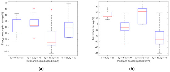
Figure 7.
The proposed eco—PPCC framework’s (a) energy consumption saving and (b) travel time saving in comparison to the Gipps model.
Figure 8 depicts the energy and time saving by the proposed eco-PPCC framework, as compared to the eco-PCC model. In terms of energy saving, as illustrated in Figure 8a, a – saving is observed in the median values. Moreover, the travel time is reduced up to , which means the travel time of both the eco-PPCC and eco-PCC models are almost the same, as shown in Figure 8b. Owing to these values, one can conclude the superiority of the eco-PPCC model when compared to the eco-PCC model.
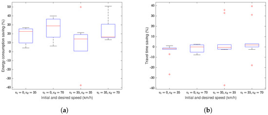
Figure 8.
The proposed eco—PPCC framework’s (a) energy consumption saving and (b) travel time saving in comparison to the eco—PCC model.
3.3. Eco-PPCC Framework Resilience in Presence of Noise
In the previous section, the simulation results of the eco-PPCC framework in a perfect data exchange were investigated. This section focuses on the circumstances in which the IPV’s upcoming data is noisy. Assuming a Gaussian noise with the average value of and an arbitrary standard deviation, , two types of negative or positive noise-caused errors may occur. Positive noises may cause collisions because the algorithm may make decisions based on a longer inter-vehicle distance. Therefore, to avoid such collisions, it is necessary to guarantee that the noise value is below a certain value. By denoting this certain value as , the probability of the noise value being lower than is equal to the surface of the hachured area in Figure 9. It can be mathematically calculated using the cumulative distribution function (CDF) of the Gaussian noise [45] as
where p is the probability of the noise values being lower than , and is the Gauss error function [45]. Using the inverse function of , the variable can be calculated as a function of p and as
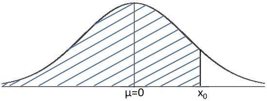
Figure 9.
A Gaussian distribution and the probability of a Gaussian variable that is smaller than .
In order to avoid collision, with the accuracy level of , the value should be added to the minimum inter-vehicle safe distance, .
The value and its corresponding energy consumption and travel time are calculated for nine different noise scenarios containing three different levels for p and , with the parameters m, m, km/h, km/h, and W. Table 4 shows the results of the simulations for each case. The values are in accordance with the error magnitude assumed in [46]. The travel time is denoted by t, and the energy consumption is denoted by E in Table 4.
Table 4.
Different noise and accuracy cases.
Figure 10 demonstrates cases 6, 7, 8, and 9 and compares them to a baseline with no noise. The behavior of case 1 is the same as the baseline, cases 2 and 4 are the same as case 7, and cases 3 and 5 are the same as case 8. Thus, for the plotting clarity, only cases 6, 7, 8, and 9 are depicted in Figure 10. The results show that the required minimum inter-vehicle safe distance increases depending on the noise magnitude and the expected safety accuracy level. An increment of either p or or both results in minor changes in travel time, energy consumption, or both. For instance, for the simulated cases in Table 4, the range of changes in travel time is from to , and the range of changes in energy consumption is from to . However, the basic trajectory of the eco-PPCC does not show significant fluctuations due to the added noise, indicating its resilience to noisy information.
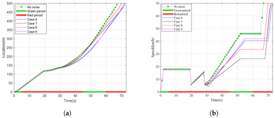
Figure 10.
(a) Location and (b) speed of noise cases 6, 7, 8, and 9 in comparison to a baseline with no noise.
4. Conclusions
This paper presents a pro-active eco-driving framework designed to regulate the speed profile of an AEV when encountering an IPV near a signalized intersection. In order to obtain a pro-active eco-driving framework rather than a reactive one, instead of using the IPV’s upcoming data in the reference trajectory tracking, the proposed eco-PPCC framework incorporates them into the reference trajectory optimization. The primary objective of this framework is to minimize the energy consumption of the AEV.
The findings indicate a significant decrease in energy consumption and the attainment of smooth and consistent speed profiles when implementing the proposed framework. Various scenario tests showed that the eco-PPCC framework significantly reduced energy consumption by up to 68.55% when compared to the baseline Gipps model, which simulates human driving behavior. Additionally, travel time savings of up to 34.51% were observed. Furthermore, the utilization of joint optimization in the up and downstream directions by the eco-PPCC framework effectively avoided unnecessary stops at intersection stop lines by adjusting the speed profile, thereby optimizing energy consumption.
As an extension of the present study, there is potential to enhance the proposed eco-PPCC framework by incorporating adjustments to the auxiliary consumption term to accommodate different levels of auxiliary power consumption in various vehicle operational modes. Additionally, future research could focus on expanding the proposed method to encompass platoons or fleets of vehicles.
Author Contributions
Conceptualization, S.H. and C.D.C.; methodology, S.H. and C.D.C.; software, S.H.; validation, S.H., C.D.C. and M.V.; formal analysis, M.V., C.D.C., E.R. and L.V.; investigation, S.H., C.D.C., E.R. and M.V.; resources, C.D.C., L.V. and T.C.; data curation, C.D.C. and T.C.; writing—original draft preparation, S.H.; writing—review and editing, S.H., M.V., C.D.C. and E.R.; visualization, S.H. and C.D.C.; supervision, M.V., C.D.C., E.R., L.V. and T.C.; project administration, L.V. and T.C.; funding acquisition, T.C. All authors have read and agreed to the published version of the manuscript.
Funding
This research was funded by SRP56: SRP-Onderzoekszwaartepunt: Autonomous Mobility & Logistics.
Institutional Review Board Statement
Not applicable.
Informed Consent Statement
Not applicable.
Data Availability Statement
Not applicable.
Conflicts of Interest
The authors declare no conflict of interest.
References
- Hao, P.; Wu, G.; Boriboonsomsin, K.; Barth, M.J. Eco-approach and departure (EAD) application for actuated signals in real-world traffic. IEEE Trans. Intell. Transp. Syst. 2018, 20, 30–40. [Google Scholar] [CrossRef]
- De Nunzio, G.; Gomes, G.; Canudas-de Wit, C.; Horowitz, R.; Moulin, P. Speed advisory and signal offsets control for arterial bandwidth maximization and energy consumption reduction. IEEE Trans. Control Syst. Technol. 2016, 25, 875–887. [Google Scholar] [CrossRef]
- Nie, Z.; Farzaneh, H. Real-time dynamic predictive cruise control for enhancing eco-driving of electric vehicles, considering traffic constraints and signal phase and timing (SPaT) information, using artificial-neural-network-based energy consumption model. Energy 2022, 241, 122888. [Google Scholar] [CrossRef]
- Han, J.; Sciarretta, A.; Ojeda, L.L.; De Nunzio, G.; Thibault, L. Safe-and eco-driving control for connected and automated electric vehicles using analytical state-constrained optimal solution. IEEE Trans. Intell. Veh. 2018, 3, 163–172. [Google Scholar] [CrossRef]
- Hooker, J.N. Optimal driving for single-vehicle fuel economy. Transp. Res. Part A Gen. 1988, 22, 183–201. [Google Scholar] [CrossRef]
- Hellström, E.; Åslund, J.; Nielsen, L. Design of an efficient algorithm for fuel-optimal look-ahead control. Control Eng. Pract. 2010, 18, 1318–1327. [Google Scholar] [CrossRef]
- Weißmann, A.; Görges, D.; Lin, X. Energy-optimal adaptive cruise control combining model predictive control and dynamic programming. Control Eng. Pract. 2018, 72, 125–137. [Google Scholar] [CrossRef]
- Asadi, B.; Vahidi, A. Predictive cruise control: Utilizing upcoming traffic signal information for improving fuel economy and reducing trip time. IEEE Trans. Control Syst. Technol. 2010, 19, 707–714. [Google Scholar] [CrossRef]
- HomChaudhuri, B.; Vahidi, A.; Pisu, P. Fast model predictive control-based fuel efficient control strategy for a group of connected vehicles in urban road conditions. IEEE Trans. Control Syst. Technol. 2016, 25, 760–767. [Google Scholar] [CrossRef]
- Liu, B.; Sun, C.; Wang, B.; Liang, W.; Ren, Q.; Li, J.; Sun, F. Bi-level convex optimization of eco-driving for connected Fuel Cell Hybrid Electric Vehicles through signalized intersections. Energy 2022, 252, 123956. [Google Scholar] [CrossRef]
- Kamal, M.A.S.; Mukai, M.; Murata, J.; Kawabe, T. Model predictive control of vehicles on urban roads for improved fuel economy. IEEE Trans. Control Syst. Technol. 2012, 21, 831–841. [Google Scholar] [CrossRef]
- Meng, X.; Cassandras, C.G. Eco-driving of autonomous vehicles for nonstop crossing of signalized intersections. IEEE Trans. Autom. Sci. Eng. 2020, 19, 320–331. [Google Scholar] [CrossRef]
- Li, S.E.; Xu, S.; Huang, X.; Cheng, B.; Peng, H. Eco-departure of connected vehicles with V2X communication at signalized intersections. IEEE Trans. Veh. Technol. 2015, 64, 5439–5449. [Google Scholar] [CrossRef]
- Kamalanathsharma, R.K.; Rakha, H.A. Leveraging connected vehicle technology and telematics to enhance vehicle fuel efficiency in the vicinity of signalized intersections. J. Intell. Transp. Syst. 2016, 20, 33–44. [Google Scholar] [CrossRef]
- Jiang, H.; Hu, J.; An, S.; Wang, M.; Park, B.B. Eco approaching at an isolated signalized intersection under partially connected and automated vehicles environment. Transp. Res. Part C Emerg. Technol. 2017, 79, 290–307. [Google Scholar] [CrossRef]
- Nie, Z.; Farzaneh, H. Role of Model Predictive Control for Enhancing Eco-Driving of Electric Vehicles in Urban Transport System of Japan. Sustainability 2021, 13, 9173. [Google Scholar] [CrossRef]
- Li, M.; Boriboonsomsin, K.; Wu, G.; Zhang, W.B.; Barth, M. Traffic energy and emission reductions at signalized intersections: A study of the benefits of advanced driver information. Int. J. Intell. Transp. Syst. Res. 2009, 7, 49–58. [Google Scholar]
- Mahler, G.; Vahidi, A. An optimal velocity-planning scheme for vehicle energy efficiency through probabilistic prediction of traffic-signal timing. IEEE Trans. Intell. Transp. Syst. 2014, 15, 2516–2523. [Google Scholar] [CrossRef]
- Wu, X.; He, X.; Yu, G.; Harmandayan, A.; Wang, Y. Energy-optimal speed control for electric vehicles on signalized arterials. IEEE Trans. Intell. Transp. Syst. 2015, 16, 2786–2796. [Google Scholar] [CrossRef]
- Tang, T.Q.; Yi, Z.Y.; Zhang, J.; Wang, T.; Leng, J.Q. A speed guidance strategy for multiple signalized intersections based on car-following model. Phys. A Stat. Mech. Its Appl. 2018, 496, 399–409. [Google Scholar] [CrossRef]
- Yang, H.; Almutairi, F.; Rakha, H. Eco-driving at signalized intersections: A multiple signal optimization approach. IEEE Trans. Intell. Transp. Syst. 2020, 22, 2943–2955. [Google Scholar] [CrossRef]
- Ma, F.; Yang, Y.; Wang, J.; Li, X.; Wu, G.; Zhao, Y.; Wu, L.; Aksun-Guvenc, B.; Guvenc, L. Eco-driving-based cooperative adaptive cruise control of connected vehicles platoon at signalized intersections. Transp. Res. Part D Transp. Environ. 2021, 92, 102746. [Google Scholar] [CrossRef]
- Wang, S.; Lin, X. Eco-driving control of connected and automated hybrid vehicles in mixed driving scenarios. Appl. Energy 2020, 271, 115233. [Google Scholar] [CrossRef]
- Sun, C.; Guanetti, J.; Borrelli, F.; Moura, S.J. Optimal eco-driving control of connected and autonomous vehicles through signalized intersections. IEEE Internet Things J. 2020, 7, 3759–3773. [Google Scholar] [CrossRef]
- He, X.; Liu, H.X.; Liu, X. Optimal vehicle speed trajectory on a signalized arterial with consideration of queue. Transp. Res. Part C Emerg. Technol. 2015, 61, 106–120. [Google Scholar] [CrossRef]
- Biggs, D.; Akcelik, R. Energy-related model of instantaneous fuel consumption. Traffic Eng. Control 1986, 27, 320–325. [Google Scholar]
- Xiang, X.; Zhou, K.; Zhang, W.B.; Qin, W.; Mao, Q. A closed-loop speed advisory model with driver’s behavior adaptability for eco-driving. IEEE Trans. Intell. Transp. Syst. 2015, 16, 3313–3324. [Google Scholar] [CrossRef]
- Chen, P.; Yan, C.; Sun, J.; Wang, Y.; Chen, S.; Li, K. Dynamic eco-driving speed guidance at signalized intersections: Multivehicle driving simulator based experimental study. J. Adv. Transp. 2018, 2018, 6031764. [Google Scholar] [CrossRef]
- Kamal, M.A.S.; Mukai, M.; Murata, J.; Kawabe, T. Ecological vehicle control on roads with up-down slopes. IEEE Trans. Intell. Transp. Syst. 2011, 12, 783–794. [Google Scholar] [CrossRef]
- Wan, N.; Vahidi, A.; Luckow, A. Optimal speed advisory for connected vehicles in arterial roads and the impact on mixed traffic. Transp. Res. Part C Emerg. Technol. 2016, 69, 548–563. [Google Scholar] [CrossRef]
- Mousa, S.R.; Ishak, S.; Mousa, R.M.; Codjoe, J. Developing an eco-driving application for semi-actuated signalized intersections and modeling the market penetration rates of eco-driving. Transp. Res. Rec. 2019, 2673, 466–477. [Google Scholar] [CrossRef]
- Guo, L.; Gao, B.; Gao, Y.; Chen, H. Optimal energy management for HEVs in eco-driving applications using bi-level MPC. IEEE Trans. Intell. Transp. Syst. 2016, 18, 2153–2162. [Google Scholar] [CrossRef]
- Han, J.; Vahidi, A.; Sciarretta, A. Fundamentals of energy efficient driving for combustion engine and electric vehicles: An optimal control perspective. Automatica 2019, 103, 558–572. [Google Scholar] [CrossRef]
- Zhang, J.; Tang, T.Q.; Yan, Y.; Qu, X. Eco-driving control for connected and automated electric vehicles at signalized intersections with wireless charging. Appl. Energy 2021, 282, 116215. [Google Scholar] [CrossRef]
- Dong, S.; Chen, H.; Gao, B.; Guo, L.; Liu, Q. Hierarchical energy-efficient control for CAVs at multiple signalized intersections considering queue effects. IEEE Trans. Intell. Transp. Syst. 2021, 23, 11643–11653. [Google Scholar] [CrossRef]
- Zhao, S.; Zhang, K. Online predictive connected and automated eco-driving on signalized arterials considering traffic control devices and road geometry constraints under uncertain traffic conditions. Transp. Res. Part B Methodol. 2021, 145, 80–117. [Google Scholar] [CrossRef]
- Deng, K.; Fang, T.; Feng, H.; Peng, H.; Löwenstein, L.; Hameyer, K. Hierarchical eco-driving and energy management control for hydrogen powered hybrid trains. Energy Convers. Manag. 2022, 264, 115735. [Google Scholar] [CrossRef]
- Dong, H.; Zhuang, W.; Chen, B.; Yin, G.; Wang, Y. Enhanced eco-approach control of connected electric vehicles at signalized intersection with queue discharge prediction. IEEE Trans. Veh. Technol. 2021, 70, 5457–5469. [Google Scholar] [CrossRef]
- Hesami, S.; De Cauwer, C.; Vafaeipour, M.; Rombaut, E.; Vanhaverbeke, L.; Coosemans, T. Bi-layer eco-driving control design of autonomous electric vehicles in presence of signalized intersections and preceding vehicles. Intell. Transp. Syst. 2023; submitted. [Google Scholar]
- Hesami, S.; De Cauwer, C.; Rombaut, E.; Vanhaverbeke, L.; Coosemans, T. Energy-Optimal Speed Control for Autonomous Electric Vehicles Up-and Downstream of a Signalized Intersection. World Electr. Veh. J. 2023, 14, 55. [Google Scholar] [CrossRef]
- Boyd, S.; Boyd, S.P.; Vandenberghe, L. Convex Optimization; Cambridge University Press: Cambridge, UK, 2004. [Google Scholar]
- Gipps, P.G. A behavioural car-following model for computer simulation. Transp. Res. Part B Methodol. 1981, 15, 105–111. [Google Scholar] [CrossRef]
- Asamer, J.; Graser, A.; Heilmann, B.; Ruthmair, M. Sensitivity analysis for energy demand estimation of electric vehicles. Transp. Res. Part D Transp. Environ. 2016, 46, 182–199. [Google Scholar] [CrossRef]
- Feng, Y.; Yu, C.; Liu, H.X. Spatiotemporal intersection control in a connected and automated vehicle environment. Transp. Res. Part C Emerg. Technol. 2018, 89, 364–383. [Google Scholar] [CrossRef]
- Papoulis, A.; Unnikrishna Pillai, S. Probability, Random Variables and Stochastic Processes; McGraw-Hill: Boston, MA, USA, 2002. [Google Scholar]
- Jia, D.; Ngoduy, D. Platoon based cooperative driving model with consideration of realistic inter-vehicle communication. Transp. Res. Part C Emerg. Technol. 2016, 68, 245–264. [Google Scholar] [CrossRef]
Disclaimer/Publisher’s Note: The statements, opinions and data contained in all publications are solely those of the individual author(s) and contributor(s) and not of MDPI and/or the editor(s). MDPI and/or the editor(s) disclaim responsibility for any injury to people or property resulting from any ideas, methods, instructions or products referred to in the content. |
© 2023 by the authors. Licensee MDPI, Basel, Switzerland. This article is an open access article distributed under the terms and conditions of the Creative Commons Attribution (CC BY) license (https://creativecommons.org/licenses/by/4.0/).