Coordinated Optimal Dispatch of Electricity and Heat Integrated Energy Systems Based on Fictitious Node Method

Abstract

In an electricity and heat integrated energy system, the transmission of thermal energy encounters significant delays, and the delays are often not integer multiples of the dispatch interval. This mismatch poses challenges for achieving coordinated dispatch with the electric power system. To address this problem, the fictitious node method is proposed in this paper, offering a novel approach to calculating the quasi-dynamic characteristics of the heating network. Furthermore, to enhance the local consumption capacity of wind power, the heat storage capacity of the heat supply network was taken into consideration in this study, and a combined energy supply model equipped with electric boilers, incorporating combined heat and power (CHP) units and gas turbine units, was developed. This model effectively expands the operational range of CHP units and enables the decoupling of electricity and heat operations in gas turbine units. The analysis conducted demonstrated the effectiveness of the proposed method and model in achieving the coordinated dispatch of electricity and heat. Moreover, it highlighted the positive impact on the overall economy of system operation and the promotion of wind power consumption. The optimal configuration presented in this paper resulted in an 8.2% improvement in system operating economics and a 38.3% enhancement in wind power integration.

1. Introduction

According to GWEC’s Global Wind Report 2023, the global cumulative installed wind power capacity reached 906 gigawatts in 2022, with an additional 77.6 gigawatts of new capacity added worldwide [1]. The rapid advancement of wind power and other emerging energy sources has generated a pressing need to accelerate the integration and consumption of these new energies. In the northern region of China, a substantial number of cogeneration facilities are in operation to fulfill the demand for winter heating. These cogeneration systems operate under the “Ordering Power by Heat” mode, which establishes a strong linkage between power generation and heating output. However, this approach results in a higher minimum power generation output to meet the system’s heating demands, leading to insufficient system peaking capacity. This scenario poses challenges for the effective consumption of new energy sources. Therefore, there is immense significance to be found in exploring the coordinated scheduling of heat and power, alongside the integration of renewable energy sources like wind power.

The electricity and heat integrated energy system is a complex network comprising two heterogeneous energy sources that are capable of achieving both economical and complementary energy utilization while efficiently reducing environmental pollution and carbon emissions [2,3,4,5,6]. Collaborative planning and operation of these energy flows can enhance the safety and stability of the system [7]. Meanwhile, the thermal energy system can provide significant flexibility to the operation of the power system and promote the consumption of renewable energy [8,9].

Liu et al. [7] investigated the steady-state operation scenario of electricity and heat networks as an integrated whole. The study employed the hydraulic–thermal model of heat networks and the electrical power flow model, utilizing the Newton–Raphson method as the solution approach. However, it did not consider the disparity in transmission characteristics between electric and thermal energy. Specifically, the electric power system exhibits remarkable transmission speeds and swift response times, whereas the thermal energy system demonstrates considerable inertia and significant transmission delays. In [6], a quasi-steady multi-energy flow model was proposed, considering the time-scale characteristics of the interactions between electricity systems and heating systems. Additionally, a heating network node-type transformation technique was developed to study the intermediate processes during the transition between steady states. Building upon this work, Pan et al. [10] quantified the quasi-dynamic interactions between electricity systems and heating systems with a focus on the transmission delay. However, it should be noted that the methods proposed in both [6,10] are inapplicable within the context of optimal scheduling.

Li et al. [11] incorporated the consideration of transmission delay into the optimal scheduling of the integrated system. In [12], the transmission delay was added to the time when the source started changing the supply temperature. Xu et al. [13] decomposed the district heating system into multiple equivalent subsystems with a single-producer–single-consumer structure for calculations. However, a significant limitation of these models is that they assume the transmission delay of the thermal system to be an integer multiple of the scheduling interval. Meeting this requirement is extremely difficult in practical systems [14], making it challenging to achieve effective coordination in scheduling between the heat and power systems. To address this issue, Wu et al. [15] proposed dividing heat users into multiple heat load zones, ensuring that the transmission delay of each zone aligns with an integer multiple of the scheduling time interval. Additionally, Gu et al. [16,17] approximated the transmission delay of the heat network by rounding it off to the nearest integer multiple of the scheduling time interval. Similarly, Wu et al. [18] rounded down the transmission delay. It is worth noting that the accuracy of calculations using these methods and the choice of the scheduling time interval are closely interconnected, often resulting in significant errors in the resulting calculations. In order to enhance computational accuracy, researchers have employed various methods such as the characteristic line model [19], the implicit upwind model [20], and the orthogonal collocation and finite difference method [21] to solve the partial differential equations describing the dynamic properties of pipes. However, Lu et al. [22] noted that the accuracy of these methods relies on the time step and space step size. Achieving a balance between computational accuracy and computational burden has proven challenging, posing difficulties when applying these methods to optimal scheduling. To address this problem, Lu et al. [22] proposed the utilization of the node method for optimal scheduling calculations, along with employing an accurate thermodynamic model to verify the obtained results.

The node method, as elaborated in [23], offers precise calculations of heat network transmission delays. This method has been widely applied in the optimal scheduling of integrated energy systems [24,25,26,27]. However, when considering both water supply network and return network delays, the node method imposes a significant computational burden. As a solution, Chen et al. [28] introduced a water mass method that employs 0–1 variables to identify the water mass delay. This approach reduces the computational complexity of the node method, albeit with a minor sacrifice in computational accuracy. Furthermore, in [29], a hydraulic–thermal cooperative optimization model based on the water mass method was proposed that takes into account the influence of hydraulics on the operation of the system.

In addition, Lu et al. [30] utilized an equivalent start network to simulate the radial district heating network. This approach gradually simplifies the network topology, starting from the load point and extending to the heat source. It results in a network that directly connects each secondary heat exchange station to the primary heat exchange station. However, the simplification of the internal states of the district heating network in the thermal inertia aggregation model introduces unavoidable errors. The experiments conducted in [30] demonstrated that these errors can be significant during specific periods. Hao et al. [31,32,33,34] employed the heat current method to model the district heating network. They applied Ohm’s law and Kirchhoff’s law to deduce the corresponding heat transport matrix and proposed a basic thermal–electric analogy circuit for each fluid element. This method represents the district heating network as an electric power network for calculation. However, it is important to note that this method may result in the loss of some valuable information during the calculation process, such as the temperature distribution along the pipe.

The analysis of the references above underscores the significance of considering the transmission process of district heating networks in the context of optimal scheduling for integrated energy systems. It is essential to develop a method that is well-suited for optimal scheduling and takes into consideration both computational accuracy and computational burden while ensuring the retention of valuable information throughout the computational process.

Combined heat and power (CHP) units and gas turbine units are commonly employed as heat sources in district heating systems. During the heating season, they often operate in a mode known as “Ordering Power by Heat,” which leads to the generation of a certain amount of forced electrical power. This forced electrical power can impose limitations on the utilization of renewable energy sources, such as wind power. To enhance the utilization of new energy sources and improve the operational flexibility of the system, several studies have explored different approaches. Nuytten et al. [35] focused on configuring heat storage tanks for CHP units, while Wu et al. [15,36] investigated the integration of heat storage tanks and electric boilers to improve the flexibility of CHP units. The impact of thermal inertia in buildings on system flexibility was analyzed in [12,16]. To further examine the effects on system flexibility, Liu et al. [25,37] simultaneously considered the use of heat storage tanks, electric boilers, thermal inertia in buildings, and the variability of heat demands. These studies investigated the individual and combined effects of these factors on system flexibility. Additionally, the influence of heat transfer constraints of heat storage equipment on system flexibility was studied in [38,39]. A district heating network reconfiguration was explored in [40] as a means to manage congestion and enhance the consumption of new energy sources. Ma et al. [41,42] discussed the conversion of electrical power into hydrogen or natural gas, which can be stored more easily, with the aim of enhancing the capacity for new energy consumption. The analysis of the aforementioned references reveals that the inclusion of energy storage equipment or the conversion of power into heat or gas, which can be more readily stored, can enhance the capacity for new energy consumption and improve the operational flexibility of the system.

Based on the aforementioned literature analysis, it is evident that scholars have presented several solutions with varying degrees of effectiveness to address the challenge of achieving coordinated dispatch of electricity and heat. However, persistent deficiencies are observed in achieving the balance between computation time and computation accuracy, as well as in effectively preserving pertinent information during the computational process. Furthermore, ongoing studies aim at enhancing the flexibility of integrated energy systems that center around energy storage configuration, the incorporation of thermal inertia within buildings, and the conversion of electricity to gas. However, these studies often overlook the significant influence of heat storage within the heating network on overall system flexibility. To address these issues, the fictitious node method is proposed in this paper as a means to calculate the quasi-dynamic model of the heating network. Unlike traditional approaches, this method offers a specific calculation time. Notably, the computational accuracy of this method is not dependent on the scheduling interval but rather closely associated with the calculation time. By employing this method, a balance between computation accuracy and complexity is struck, while also retaining essential information, such as the temperature distribution along the pipeline. Additionally, based on the advantages of the fictitious node method, a methodology for quantifying the heat storage capacity of the heating network is proposed. Moreover, the heat storage capacity within the heating network was taken into full consideration in this study. A portion of the forced electrical power generated by CHP units and gas turbine units was converted into thermal energy through electric boilers. This thermal energy was then stored using the heat storage capacity of the heating network, thereby improving the flexibility of system operation and enhancing the local consumption capacity of wind power.

2. Quasi-Dynamic Mode of the Heating Network

The heating system usually operates in two regulation modes: quality regulation mode and quantity regulation mode [43]. The quality regulation mode refers to maintaining a constant mass flow while varying the temperature supply [17]. On the other hand, the quantity regulation mode refers to adjusting the mass flow while keeping the temperature supply constant [43]. Due to its stable hydraulic properties, the quality regulation mode is more commonly used in practical engineering [11,16]. Therefore, this study was based on the quality regulation mode.

Several assumptions were made for the heating network [44]:

(1)

Water in the pipe network was considered an incompressible fluid.

(2)

Friction heat was neglected.

(3)

The thermal properties of the water were assumed to be constant.

(4)

Turbulence effects were ignored, and the water flow in the pipeline was assumed to be stable.

(5)

The longitudinal temperature distribution of the water flow was disregarded, and only the axial direction of the water flow temperature was considered.

The centralized heat supply system consists of the heat source, primary heat exchange station, primary network, secondary heat exchange stations, secondary network, and heat users. This study specifically focused on the primary network, which serves as a long-distance transport network characterized by significant transmission delays and dynamic properties. In contrast, the secondary network functions as a distribution network with shorter transmission delays and less pronounced dynamic characteristics [10]. Consequently, the secondary network is not addressed in this paper. The thermal flow model of the primary network is depicted in Figure 1. The return water passes through the primary heat exchange station, where it is heated by the heat source. Subsequently, the water, now at an elevated temperature, enters the water supply network and is distributed to each secondary heat exchange station. Finally, after undergoing heat exchange, the water flows back into the water return network. Throughout the transmission process, the water experiences transmission delays and incurs losses.

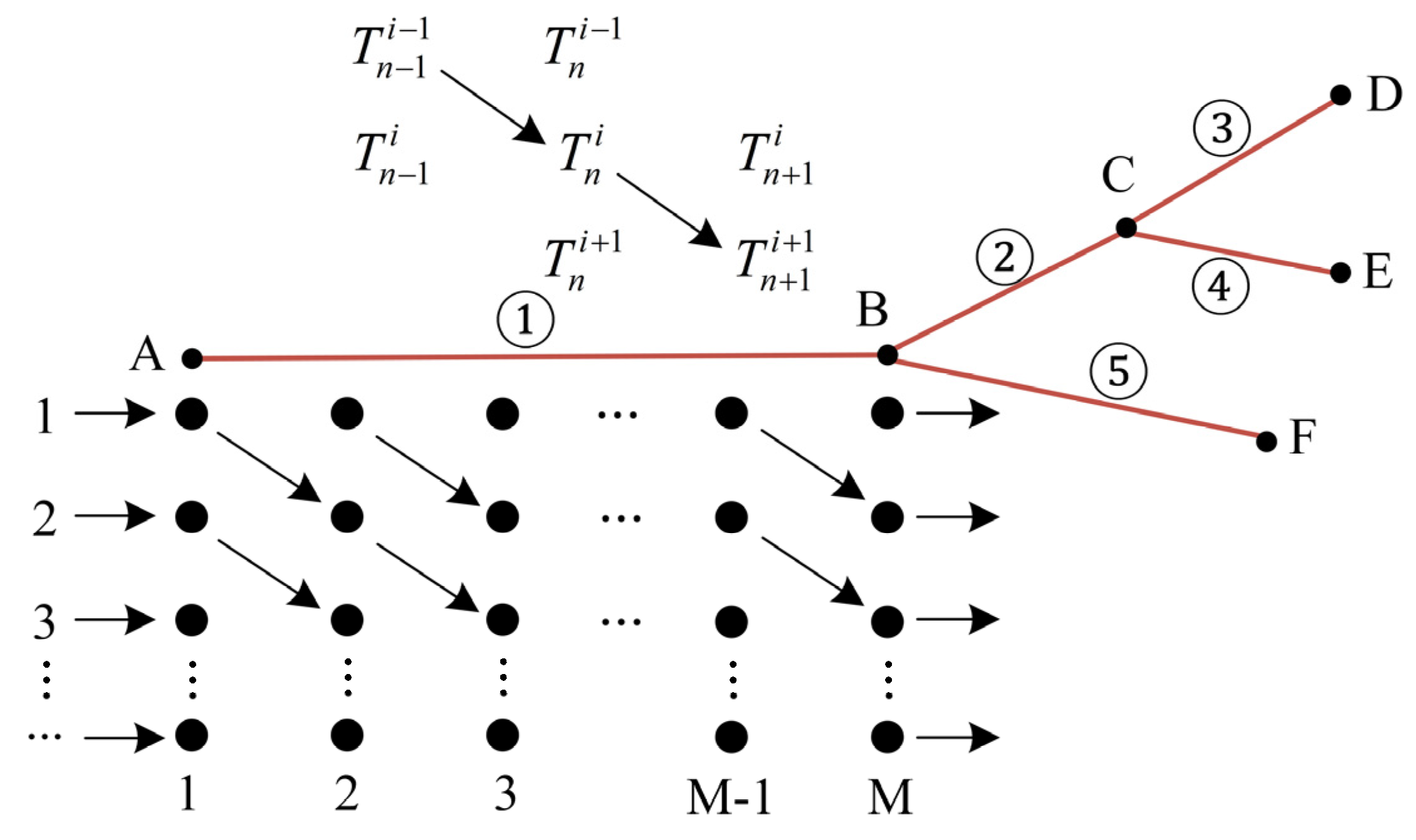
2.1. The Fictitious Node Method

The transmission delay of the pipe can be calculated by using (1):

$$\tau =\frac{\pi \rho d^{2}L}{4m}$$

(1)

where τ is the transmission delay, ρ is the density of water, d is the inner diameter of the pipe, L is the length of the pipe, and m is the mass flow rate of the water.

The thermal loss, referred to as a temperature loss, experienced by water following its passage through a pipeline can be calculated using Equation (2) [8,14]:

$$T_x=T_0+(T_{in}-T_0)\exp (-\frac{\pi x\alpha d}{c_{w}m})$$

(2)

where T₀, T_in, and T_x represent the ambient temperature surrounding the pipe, the initial temperature of the hot water at the entry point of the pipe, and the temperature of the hot water at a distance x from the entry point of the pipe, respectively; α is the total heat transfer coefficient between the interior of the pipe and its surroundings; and c_w is the specific heat capacity of water.

Given that pipelines are typically buried underground, the immediate surrounding medium is soil. The standardization of burial depth for directly buried heat pipes dictates a minimum depth of 0.7 m [45]. Furthermore, at depths greater than 0.4 m, diurnal fluctuations in soil temperature display negligible variation [46]. Thus, treating T₀ as a constant within this context is warranted [14].

The fictitious node method is presented below as an example of a six-node heating network, as illustrated in Figure 2. Point A is connected to the primary heat exchange station, while points D, E, and F are connected to their respective secondary heat exchange stations. This network exemplifies a typical branch heating network, featuring the pipe that connects to the primary heat exchange station, pipes that connect to the secondary heat exchange stations, and intermediate pipes.

To ensure accurate calculations, it is important to establish a suitable calculation time, denoted as δt, that is a factor of the scheduling interval Δt. Transform the transmission delay of each pipe in the entire heating network using (3).

$$\{\begin{array}{l}{\tau }_1^{\prime }=\left(\mathrm{round}\right[{\tau }_1/\mathsf{\delta }t\left]\right)\mathsf{\delta }t\hfill \\ {\tau }_2^{″}={\tau }_2+{\tau }_1-{\tau }_1^{\prime }\hfill \\ {\tau }_5^{″}={\tau }_5+{\tau }_1-{\tau }_1^{\prime }\hfill \\ {\tau }_2^{\prime }=\left(\mathrm{round}\right[{\tau }_2^{″}/\mathsf{\delta }t\left]\right)\mathsf{\delta }t\hfill \\ {\tau }_5^{\prime }=\left(\mathrm{round}\right[{\tau }_5^{″}/\mathsf{\delta }t\left]\right)\mathsf{\delta }t\hfill \\ {\tau }_3^{″}={\tau }_3+{\tau }_2^{″}-{\tau }_2^{\prime }\hfill \\ {\tau }_4^{″}={\tau }_4+{\tau }_2^{″}-{\tau }_2^{\prime }\hfill \\ {\tau }_3^{\prime }=\left(\mathrm{round}\right[{\tau }_3^{″}/\mathsf{\delta }t\left]\right)\mathsf{\delta }t\hfill \\ {\tau }_4^{\prime }=\left(\mathrm{round}\right[{\tau }_4^{″}/\mathsf{\delta }t\left]\right)\mathsf{\delta }t\hfill \end{array}$$

(3)

where round[·] indicates the process of rounding the values within the square brackets, τ represents the original transmission delay of a pipeline, τ″ represents the intermediate calculation of the pipeline transmission delay, τ′ represents the transformed transmission delay of a pipe, and the subscript denotes the respective pipe number.

The transformation method for the transmission delay of pipe j can be summarized using Equation (4):

$$\{\begin{array}{l}{\tau }_j^{″}={\tau }_j+{\tau }_{j,p}-{\tau }_{j,p}^{\prime }\hfill \\ {\tau }_j^{\prime }=\left(\mathrm{round}\right[{\tau }_j^{″}/\mathsf{\delta }t\left]\right)\mathsf{\delta }t\hfill \end{array}$$

(4)

where τ_j and τ_j,p are the original transmission delays of pipe j and the pipe before pipe j, respectively; ${\tau }_j^{\prime }$ and ${\tau }_{j,p}^{\prime }$ are the transformed transmission delays of pipe j and the pipe before pipe j, respectively; and ${\tau }_j^{″}$ is an intermediate variable of pipe j in the computation of ${\tau }_j^{\prime }$. It is important to note that when pipe j is connected to a primary heat exchange station, such as pipe 1 in Figure 2, it implies that there is no previous pipe for this pipe and that ${\tau }_j^{″}$ = τ_j.

The transformed length of each pipe can be calculated by using (5):

$$L_j^{\prime }={\tau }_j^{\prime }\frac{4m_j}{\pi \rho d_j^2}$$

(5)

where the subscript j denotes the number of the respective pipe and $L_j^{\prime }$ is the transformed length of the pipe numbered j.

Up to this point, it has been ensured that the transmission delay of each pipe is a multiple of the calculation time δt. Within the entire heating network, the primary and secondary heat exchange stations, as well as the pipeline connections, are positioned at a hypothetical node. Consequently, the calculation of the transmission delay for the entire network and the temperature distribution along the pipeline becomes straightforward. Figure 2 illustrates this concept, using pipeline 1 as an example. Assuming that the transformed length of the pipe results in a transmission delay equivalent to M-1 times the calculation time, M fictitious nodes are established along pipe 1, and these fictitious nodes encompass both ends of the pipe.

The distance l_j between two neighboring fictitious nodes on pipe j can be calculated by using (6):

$$l_j=\mathsf{\delta }t\frac{4m_j}{\pi \rho d_j^2}$$

(6)

The temperature distribution along the water supply and return pipes denoted by subscript j can be calculated by using (7) and (8):

$$T_{n+1,s,j}^{i+1}=T_0+(T_{n,s,j}^i-T_0)\exp (-\frac{\pi \alpha d_j{l}_j}{c_w{m}_j})$$

(7)

$$T_{n,r,j}^{i+1}=T_0+(T_{n+1,r,j}^i-T_0)\exp (-\frac{\pi \alpha d_j{l}_j}{c_w{m}_j})$$

(8)

where $T_{n,s,j}^i$ is the temperature of the water supply pipe numbered j at calculation time numbered i and fictitious node numbered n and $T_{n+1,r,j}^i$ is the temperature of return pipe j at calculation time i and fictitious node n + 1.

2.2. Heat Flow Model

For a node connected by different pipes, the mass flow rate of water entering the node is equal to the mass flow rate of water exiting the node. This relationship can be mathematically expressed as (9):

$${\displaystyle \sum _{j\in In(k)}{m}_j=}{\displaystyle \sum _{j\in Out(k)}{m}_j}$$

(9)

where In(k) and Out(k) represent the sets of pipes connected to node k that carry flow into and out of the node, respectively.

For a node connected by different pipes, water of varying temperatures enters the node for temperature mixing and subsequently exits the node at the same temperature. In this process, the heat energy entering the node equals the heat energy leaving the node. The calculation of temperature mixing is determined by (10):

$${\displaystyle \sum _{j\in In(k)}{T}_{out,j}^t{m}_j=}{T}_k^t{\displaystyle \sum _{j\in Out(k)}{m}_j}$$

(10)

where $T_{out,j}^t$ is the temperature at the outlet of pipe j at time t; $T_k^t$ is the temperature at node k after temperature mixing at time t and also denotes the temperature at the inlet of the pipes flowing out of node k at time t.

The primary heat exchange station is responsible for heating the returning water from the pipe network and supplying it to the water supply network. In accordance with the law of conservation of energy, the heat exchange power of the primary heat exchange station can be calculated by using (11):

$$H_p^t=c_w{m}_p{\displaystyle \sum _{i=1}^{i=\Delta t/\mathsf{\delta }t}(T_{in,s}^i-T_{out,r}^i)}/(\Delta t/\mathsf{\delta }t)$$

(11)

where $H_p^t$ represents the heat transfer power of the primary heat exchange station at time t, m_p is the mass flow rate of the primary heat exchange station, $T_{in,s}^i$ is the temperature at the inlet of the water supply pipe connected to the primary heat exchange station at time i, and $T_{out,r}^i$ is the temperature at the outlet of the return pipe connected to the primary heat exchange station at time i.

A secondary heat exchange station receives thermal energy transferred from the primary network and further distributes it to the secondary network for delivery to the heat users. The heat exchange power of the secondary heat exchange stations can be calculated using (12):

$$H_d^t={\displaystyle \sum _{q=1}^{q=\mathrm{v}}[c_w{m}_q{\displaystyle \sum _{i=1}^{i=\Delta t/\mathsf{\delta }\mathrm{t}}(T_{out,s,q}^i-T_{in,r,q}^i)/(\Delta t/\mathsf{\delta }t)}]}$$

(12)

where $H_d^t$ is the total heat exchange power of v secondary heat exchange stations at time t, m_q is the mass flow rate of the qth secondary heat exchange station, $T_{out,s,q}^i$ is the temperature at the outlet of the water supply pipe connected to the qth secondary heat exchange station at time i, and $T_{in,r,q}^i$ is the temperature at the inlet of the return pipe connected to the qth secondary heat exchange station at time i.

The temperature limits for the heating network are represented by (13) and (14):

$$T_s^{\min }\le T_{n,s,j}^t\le T_s^{\max }$$

(13)

$$T_r^{\min }\le T_{n,r,j}^t\le T_r^{\max }$$

(14)

where $T_{n,s,j}^t$ is the temperature of water supply pipe j at fictitious node n and time t; $T_s^{\min }$ and $T_s^{\max }$ are the maximum and minimum allowable temperatures in the water supply network, respectively; and the subscript r denotes the return pipe.

To ensure the safe and stable operation of the heating network, it is necessary to impose constraints on the rate of temperature change in the pipe network. This can be achieved by controlling the rate of temperature change at the inlet of the supply and return network, as expressed in (15) and (16):

$$\left|T_{in,s}^t-T_{in,s}^{t+1}\right|\le \Delta T_{in,s}^{\max }$$

(15)

$$\left|T_{in,r,q}^t-T_{in,r,q}^{t+1}\right|\le \Delta T_{in,r}^{\max }$$

(16)

where $\Delta T_{in,s}^{\max }$ is the maximum allowable temperature change at the inlet of the water supply pipe connecting the primary heat exchange station between time t and t + 1; $\Delta T_{in,r}^{\max }$ is the maximum allowable temperature change at the inlet of the return pipe connecting each secondary heat exchange station between time t and t + 1.

The quasi-dynamic model of the heating network can be established through Equations (1)–(16). The determination of the scheduling interval for the system typically relies on the system’s operational requirements and load forecast data. For the thermal system, the day-ahead scheduling interval commonly assumes values of 15 min, 30 min, or 1 h. Within each scheduling interval, an assumption is made regarding the constancy of the heat load demand. This assumption implies that the heat exchange power of the secondary heat exchange station remains constant, as indicated in Equation (11). Simultaneously, the heat source output is determined through optimal scheduling, while the heat exchange power of the primary heat exchange station also remains constant within a given scheduling interval, as expressed in Equation (12). Regarding the source and load powers, the entire system operates under the framework of steady-state scheduling. However, the presence of transmission delays within the heating network introduces dynamic characteristics to the hot water transmission process. To address this dynamic behavior, a calculation time was introduced, which is consistently set to the factor of the scheduling interval. This selected calculation time enables a more precise analysis of the transmission characteristics of the heating network at a finer time scale. The alteration in temperature of the return water is depicted by employing the calculation time as the temporal scale. The return water sequentially passes through the primary heat exchange station, having undergone an identical temperature increase within a given scheduling interval, and subsequently enters the water supply pipeline. This principle equally applies to the secondary heat exchange station. This method seeks to achieve a more accurate calculation of the heat transmission process through quasi-dynamic modeling, aiming to enhance the coordinated scheduling of heat and power.

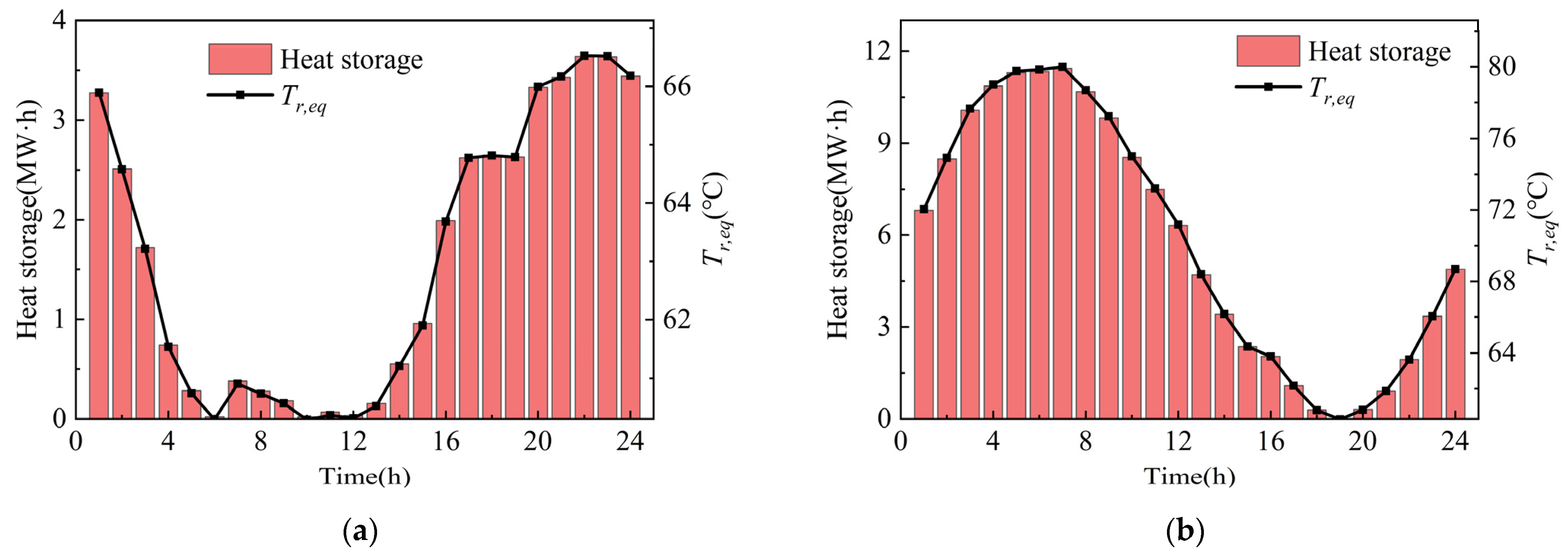
2.3. Quantification of Heat Storage in the Heating Network

The transmission delay effect in the thermal system allows the heating network to possess a certain heat storage potential. This potential capacity can be utilized when the supply and return water temperatures can be adjusted. The heat storage capacity of the heating system is indicated by changes in the return water temperature. During a specific time period, if the heat output from the heat source exceeds the corresponding heat load demand, heat is transmitted through the pipe network and exchanged at secondary heat transfer stations, resulting in an increase in the temperature of the return water network, indicating heat storage within the pipe network. Conversely, a decrease in the return water temperature indicates heat release from the pipe network. Heat storage in a heating network resembles a heat storage tank, as both contribute to enhanced system operational economics. However, the distinct advantage of employing heat storage in the heating network lies in its avoidance of the need for additional equipment configuration, resulting in a cost reduction. Moreover, while employing heat storage tanks, it is crucial to account for the impact of heat transmission delays. In comparison, the utilization of heating network heat storage offers superior flexibility. Due to temperature fluctuations, the heat storage capacity of the network at any given moment cannot be accurately determined by observing the temperature at a single location. To better quantify the heat storage, the return water equivalent average temperature is defined by (17):

$$T_{r,eq}^t=[{\displaystyle \sum _{j=1}^{\mathrm{R}}{\displaystyle \sum _{n=1}^{{\mathrm{M}}_j-1}(\frac{T_{n,r,j}^t+T_{n+1,r,j}^t}{2}{l}_j}}\frac{\pi d_j^2}{4})]/({\displaystyle \sum _{j=1}^{\mathrm{R}}\frac{\pi d_j^2{l}_j({\mathrm{M}}_j-1)}{4}})$$

(17)

where $T_{r,eq}^t$ is the equivalent average temperature of the return pipe network at time t, R is the total number of pipes, and M_j is the number of fictitious nodes of pipe j.

The magnitude of heat storage in the heating network can be calculated by using (18):

$$S_h^t=c_w{m}_{\Sigma }(T_{r,eq}^t-T_{r,eq}^{\min })$$

(18)

where $S_h^t$ is the amount of heat stored in the heating network at time t, m_Σ is the total water mass in the return pipe network, and $T_{r,eq}^{\min }$ is the minimum equivalent average temperature of the return network.

3. Optimal Dispatch Model of the System

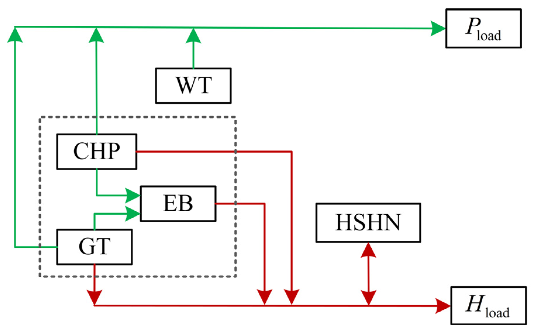
3.1. Structure of the System

An integrated energy system typically consists of five components: source, network, load, storage, and energy conversion equipment. In this study, the model of the electricity and heat integrated energy system is presented in Figure 3. The energy supply equipment includes wind turbines (WTs), CHP units, and gas turbine (GT) units. Electric boilers (EBs) are used as energy conversion equipment. The CHP, GTs, and EBs together form a combined energy supply model. In terms of the energy supply network, this study focused on the dynamic characteristics of the heating network and the heat storage in the heating network (HSHN), given the quick response time of the power system. This emphasis was made to highlight the key aspects of the study.

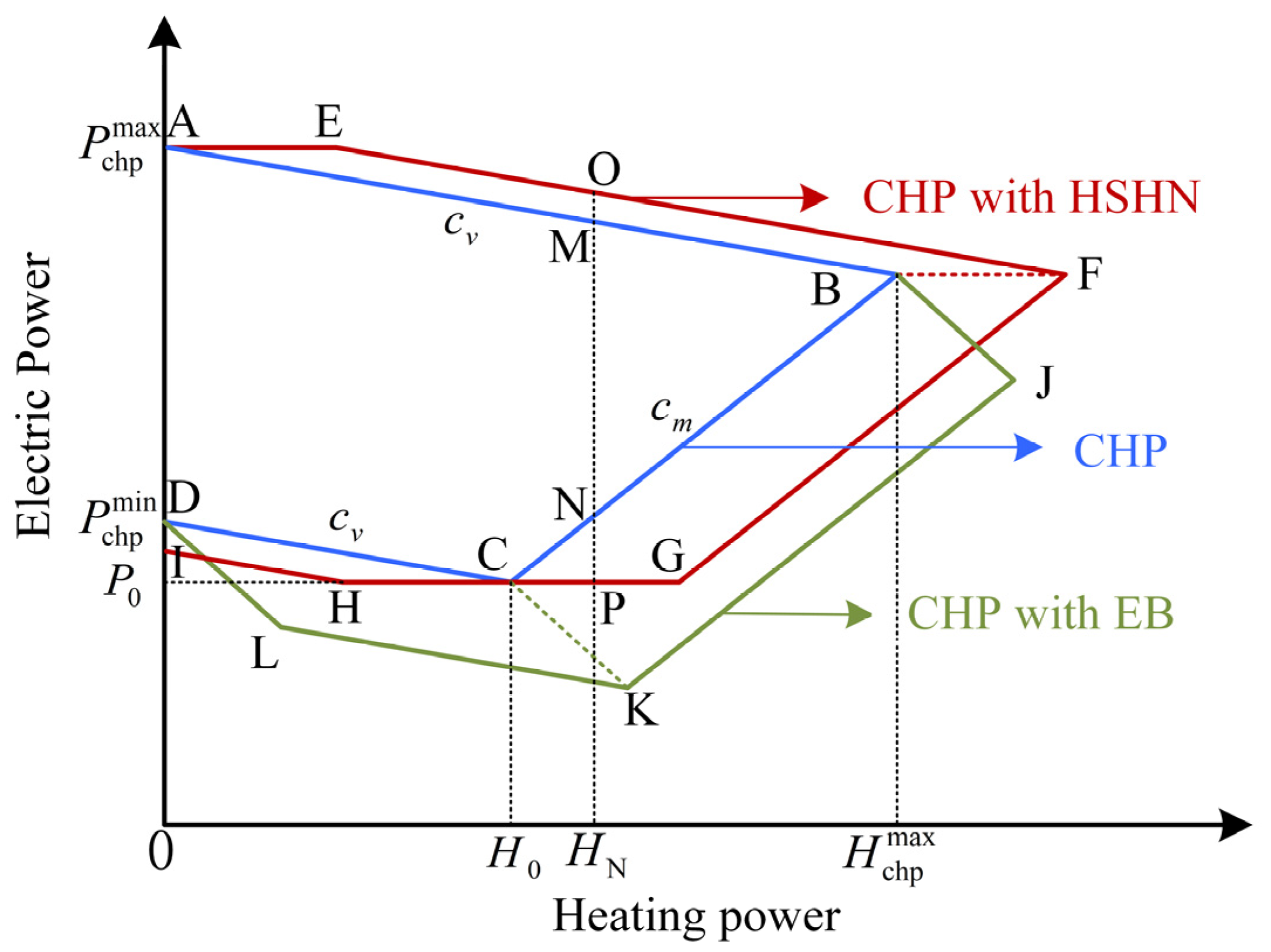
3.2. Modeling of the Equipment

CHP and GT were the two cogeneration units under investigation in this study. The CHP operates as an extraction condensing unit. Here, a portion of the steam that has not completed its intended work is extracted from the turbine’s extraction port and allocated to the heat users. The remaining steam continues its work within the turbine before being released into the condenser, where it transforms into water and subsequently recirculates to the boiler. In the event of a sudden reduction in heat load, the surplus steam can further expand, generating electricity beyond the stage following the turbine’s extraction point. The key advantage of this unit lies in its enhanced flexibility, enabling it to effectively cater to a wide range of both thermal and electrical load requirements. On the other hand, the GT operates as a back-pressure unit, characterized by a discharge pressure exceeding atmospheric pressure. It demonstrates favorable economics under designed operating conditions, manifesting pronounced energy-saving effects. Noteworthy attributes include fewer stages, yielding a simple and reliable structure. This unit obviates the necessity for an extensive condenser, resulting in a lightweight, compact profile and reduced costs. When the exhaust steam is employed for the heat supply, the unit maximizes the utilization of heat energy, achieving heightened energy efficiency compared with the CHP unit. However, it is important to note that the power output of the turbine becomes directly correlated with the heat supply load. As a result, power generation hinges on the heat supply, lacking independent adjustability to concurrently meet the demands of both heat and electricity consumers.

The operating characteristics of the CHP are depicted in Figure 4. The operating range of the pumped CHP is denoted by the boundary ABCD, which can be mathematically expressed using (19)–(21):

$$\max \left\{P_{\mathrm{chp}}^{\min }-c_v{H}_{\mathrm{chp}}^t, c_m(H_{\mathrm{chp}}^t-H_0)+P_0\right\}\le P_{\mathrm{chp}}^t\le P_{\mathrm{chp}}^{\max }-c_v{H}_{\mathrm{chp}}^t$$

(19)

$$H_{\mathrm{chp}}^t\ge 0$$

(20)

$$R_{\mathrm{chp}}^{\mathrm{D}}\le P_{\mathrm{chp}}^t-P_{\mathrm{chp}}^{t+1}\le R_{\mathrm{chp}}^{\mathrm{U}}$$

(21)

where $P_{\mathrm{chp}}^t$ is the electric power output of the CHP at time t, $H_{\mathrm{chp}}^t$ is the heating power output of CHP at time t, $P_{\mathrm{chp}}^{\min }$ and $P_{\mathrm{chp}}^{\max }$ are respectively the minimum and maximum electric power output of CHP in pure condensation state, c_v is the value of the reduction in electric power output per unit of heating power output increased by cogeneration for a fixed steam intake, c_m is the linear supply slope of heating power and electric power, H₀ is the thermal power with the minimum electrical power P₀, and $R_{\mathrm{chp}}^{\mathrm{D}}$ and $R_{\mathrm{chp}}^{\mathrm{U}}$ are the CHP downward and upward climbing power, respectively.

AEFGHI represents the comprehensive external operating characteristics of the CHP when considering the HSHN. Here, AEFGCB refers to the range for heat release, where the length of AE or BF (AE = BF) indicates the maximum heat release power size. Additionally, DCHI represents the range for heat storage, and the length of HC signifies the maximum heat storage power capacity. The regulation range of electric power is expanded from [P_N,P_M] to [P_O,P_P] when the heating power is H_N, significantly enhancing the flexibility of the operation of the CHP.

ABJKLD illustrates the comprehensive external operating characteristics of the CHP with the addition of an EB. The aim is to enhance wind power consumption capacity during periods of low load demand. To achieve this, a portion of the CHP electric output is converted to heat by the EB, effectively reducing the minimum forced output of the CHP. The CHP electric power output can be divided into two parts by using (22) and (23):

$$P_{\mathrm{chp}}^t=P_{\mathrm{chp}1}^t+P_{\mathrm{chp}2}^t$$

(22)

$$0\le P_{\mathrm{chp}1}^t\le P_{\mathrm{chp}}^t$$

(23)

where $P_{\mathrm{chp}1}^t$ is the electrical power for supplying the power grid at time t and $P_{\mathrm{chp}2}^t$ is the electrical power input to the EB emitted by the CHP at time t.

The operating characteristics of an EB can be expressed by (24) and (25):

$$H_{\mathrm{eb}}^t={\eta }_{\mathrm{eb}}{P}_{\mathrm{eb}}^t$$

(24)

$$0\le P_{\mathrm{eb}}^t\le P_{\mathrm{eb}}^{\max }$$

(25)

where $H_{\mathrm{eb}}^t$ is the output thermal power of the EB at time t, $P_{\mathrm{eb}}^t$ is the input electric power of the EB at time t, η_eb is the energy conversion efficiency of the EB, and $P_{\mathrm{eb}}^{\max }$ is the maximum input electric power of the EB.

The operating characteristics of the GT can be expressed by (26)–(28):

$$H_{\mathrm{gt}}^t={\beta }_{\mathrm{gt}}{P}_{\mathrm{gt}}^t$$

(26)

$$P_{\mathrm{gt}}^{\min }\le P_{\mathrm{gt}}^t\le P_{\mathrm{gt}}^{\max }$$

(27)

$$R_{\mathrm{gt}}^{\mathrm{D}}\le P_{\mathrm{gt}}^t-P_{\mathrm{gt}}^{t+1}\le R_{\mathrm{gt}}^{\mathrm{U}}$$

(28)

where β_gt is the thermoelectric ratio of the GT; $P_{\mathrm{gt}}^t$ and $H_{\mathrm{gt}}^t$ are the electrical and thermal power output of GT, respectively; $P_{\mathrm{gt}}^{\max }$ is the maximum output electrical power of the GT; and $R_{\mathrm{gt}}^{\mathrm{D}}$ and $R_{\mathrm{gt}}^{\mathrm{U}}$ are the GT downward and upward climbing power, respectively.

The electric power output of GT can be divided into two parts using (29) and (30):

$$P_{\mathrm{gt}}^t=P_{\mathrm{gt}1}^t+P_{\mathrm{gt}2}^t$$

(29)

$$0\le P_{\mathrm{gt}1}^t\le P_{\mathrm{gt}}^t$$

(30)

where $P_{\mathrm{gt}1}^t$ is the electrical power for supplying the power grid at time t and $P_{\mathrm{gt}2}^t$ is the electrical power input to the EB emitted by the GT at time t.

3.3. Objective Function and Constraints

The minimum operating cost serves as the objective function for the optimal scheduling of the system, and its calculation is based on (31)–(34):

$$f_{\Sigma }=C_{\mathrm{chp}}+C_{\mathrm{gt}}+C_{\mathrm{aw}}$$

(31)

$$C_{\mathrm{chp}}={\displaystyle \sum _{t=1}^{24}[a_0+a_1(P_{\mathrm{chp}}^t+c_v{H}_{\mathrm{chp}}^t)+a_2{(P_{\mathrm{chp}}^t+c_v{H}_{\mathrm{chp}}^t)}^2]}$$

(32)

$$C_{\mathrm{gt}}={\displaystyle \sum _{t=1}^{24}{b}_1{P}_{\mathrm{gt}}^{\mathrm{t}}}$$

(33)

$$C_{\mathrm{aw}}={\displaystyle \sum _{t=1}^{24}{w}_1}{P}_{\mathrm{aw}}^t$$

(34)

where f_Σ is the total costs; C_chp, C_gt, and C_aw are the operating costs of the CHP and GT and wind abandonment penalty costs, respectively; $P_{\mathrm{aw}}^t$ is the abandoned wind power at time t; and a₀, a₁, a₂, b₁, and w₁ are the cost factors.

The constraints for wind power are expressed as (35) and (36):

$$P_{\mathrm{w}}^t=P_{\mathrm{c}\mathrm{w}}^t+P_{\mathrm{aw}}^t$$

(35)

$$0\le P_{\mathrm{c}\mathrm{w}}^t\le P_{\mathrm{w}}^t$$

(36)

where $P_{\mathrm{w}}^t$ and $P_{\mathrm{c}\mathrm{w}}^t$ are the power generated by the WT and consumed by the grid, respectively.

The electric power balance constraints for system operation are expressed as (37) and (38):

$$P_{\mathrm{chp}1}^t+P_{\mathrm{gt}1}^t+P_{\mathrm{cw}}^t=P_{\mathrm{load}}^t$$

(37)

$$P_{\mathrm{eb}}^t=P_{\mathrm{chp}2}^t+P_{\mathrm{gt}2}^t$$

(38)

where $P_{\mathrm{load}}^t$ is the electric load at time t.

The thermal power balance constraint at the heat source is expressed as (39):

$$H_{\mathrm{chp}}^t+H_{\mathrm{gt}}^t+H_{\mathrm{eb}}^t=H_p^t$$

(39)

The thermal power balance constraint at the heat load is expressed as (40):

$$H_{\mathrm{load}}^t=H_d^t$$

(40)

where $H_{\mathrm{load}}^t$ is the heat load at time t.

The constraints of the heating network are expressed as (4)–(16).

4. Case Studies

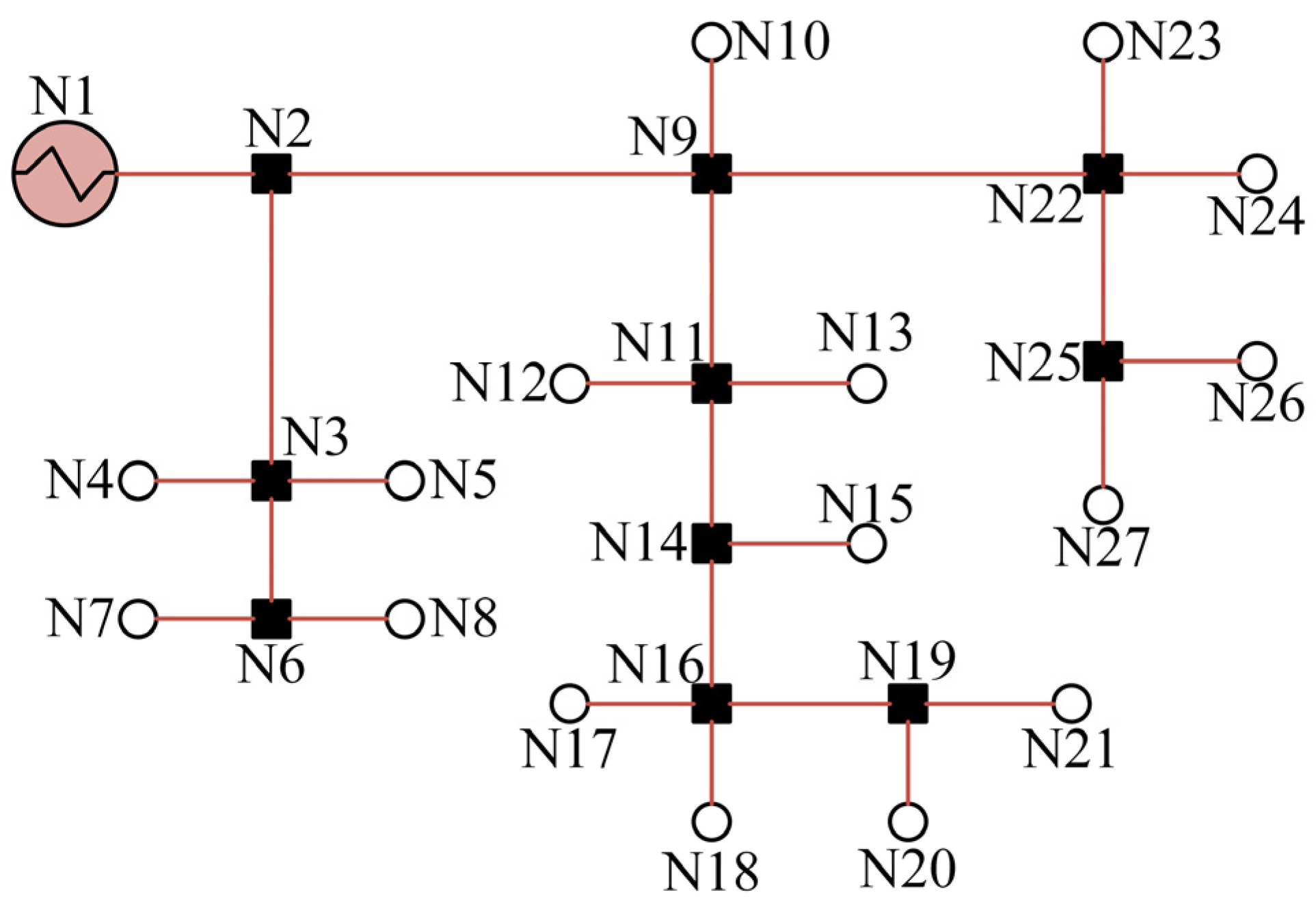
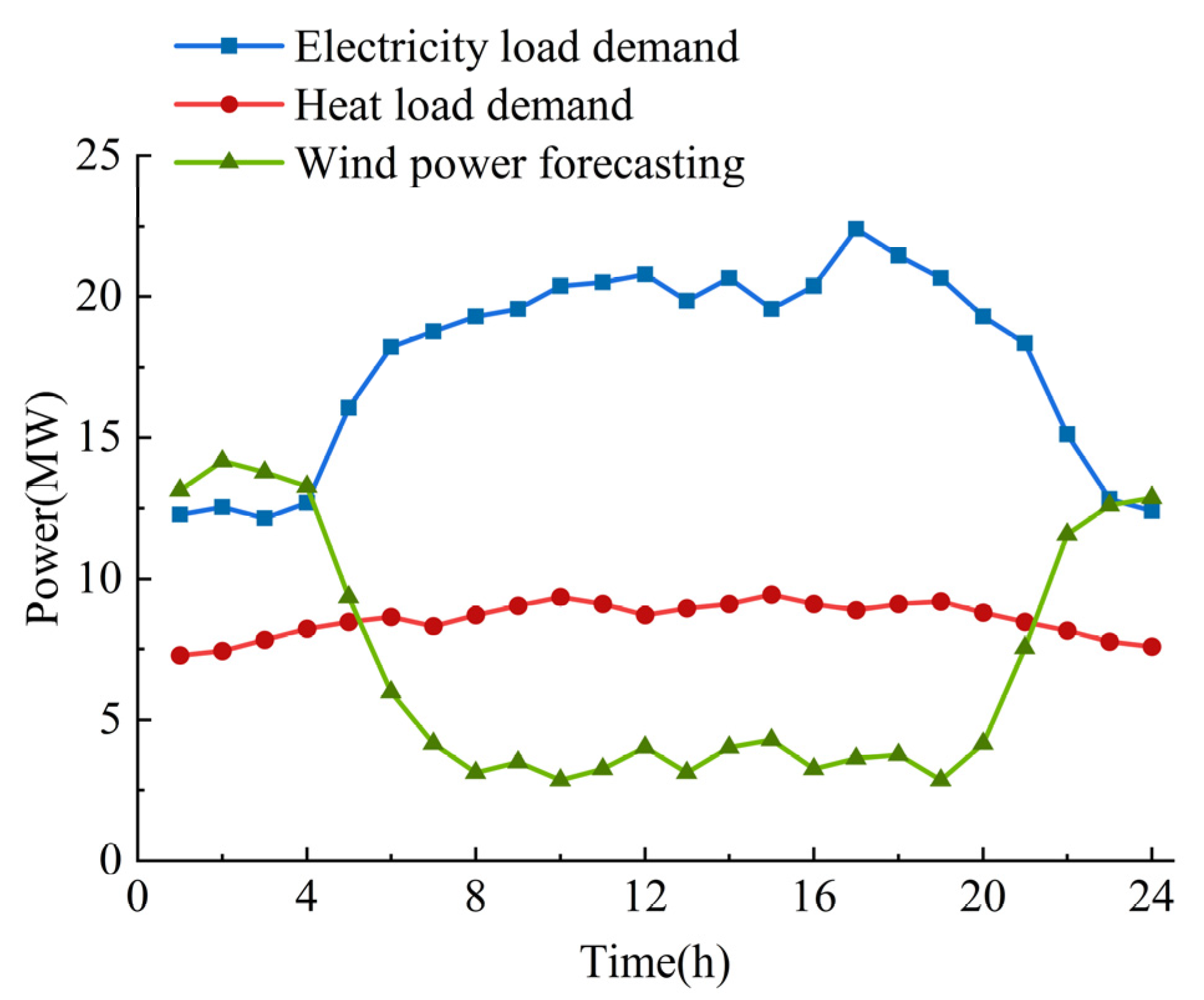
4.1. The Setup of the Simulation

In this study, the integrated energy system structure depicted in Figure 3 and the 27-node heating network shown in Figure 5 were employed for the case studies. The parameters of the heating network are presented in

Table 1. Parameters of the heating network.

Pipeline	L (m)	d (m)	m (kg/s)	Pipeline	L (m)	d (m)	m (kg/s)
1–2	350	0.5	128	14–15	400	0.15	8
2–3	900	0.3	32	14–16	300	0.3	32
3–4	350	0.15	8	16–17	300	0.15	8
3–5	350	0.15	8	16–18	450	0.15	8
3–6	300	0.2	16	16–19	450	0.2	16
6–7	500	0.15	8	19–20	500	0.15	8
6–8	500	0.15	8	19–21	500	0.15	8
2–9	700	0.4	96	9–22	600	0.3	32
9–10	400	0.15	8	22–23	250	0.15	8
9–11	500	0.3	56	22–24	400	0.15	8
11–12	400	0.15	8	22–25	400	0.2	16
11–13	400	0.15	8	25–26	300	0.15	8
11–14	400	0.3	40	25–27	400	0.15	8

, and the operating parameters of the system are provided in

Table 2. Parameters of the system scheduling operation.

Parameters	Values	Parameters	Values	Parameters	Values	Parameters	Values
$P_{\mathrm{chp}}^{\min }$ (MW)	7	$P_{\mathrm{chp}}^{\max }$ (MW)	15	ηeb	0.95	T0 (°C)	0
H0 (MW)	5	P0 (MW)	6	α (W/(m2·°C))	0.65	cw (J/(kg·°C))	4200
cv	0.2	cm	0.8	ρ (kg/m3)	1000	$T_s^{\min }$ (°C)	70
$R_{\mathrm{chp}}^{\mathrm{D}}$ (MW/h)	−5	$R_{\mathrm{chp}}^{\mathrm{U}}$ (MW/h)	5	$T_s^{\max }$ (°C)	100	$T_r^{\min }$ (°C)	60
$P_{\mathrm{gt}}^{\min }$ (MW)	2	$P_{\mathrm{gt}}^{\max }$ (MW)	10	$T_r^{\max }$ (°C)	80	a0 (USD/MW)	13.29
βgt	1.05	$R_{\mathrm{gt}}^{\mathrm{D}}$ (MW/h)	−3	a1 (USD/MW2)	0.044	a2 (USD/MW)	39
$R_{\mathrm{gt}}^{\mathrm{U}}$ (MW/h)	3	$P_{\mathrm{eb}}^{\max }$ (MW)	10	b1 (USD/MW)	70	w1 (USD/MW)	7

. Furthermore, the load demand curve and wind power forecasting curve are illustrated in Figure 6. The model presented in this paper was a linear model, which was solved by invoking the optimization solver Cplex through Matlab. The solution process took place on a laptop equipped with an AMD Ryzen 7 5800 H processor and 16 GB of RAM.

To validate the effectiveness of the proposed model, the following four optimization scheduling cases were established:

Case 1: Considering the HSHN and the EB.

Case 2: Considering the HSHN but without the EB.

Case 3: Without considering the HSHN but with the EB.

Case 4: Without considering the HSHN and without the EB.

4.2. Selection of the Calculation Time and Validation of the Effectiveness of the Fictitious Node Method

To enhance the selection of the calculation time, a constant temperature of hot water was assumed to continuously flow into the heating network from the first node of the water supply pipe. In this study, this temperature was assumed to be 90 °C. It is essential to note that different assumed temperatures will only affect the absolute error and will not impact the relative error. By comparing the transmission delay error and temperature loss error from the primary heat exchange station to each secondary heat exchange station before and after transforming the lengths of the pipes, the error values were obtained and are presented in

Table 3. The choice of calculation time and the magnitude of error.

	1 min	2 min	5 min	6 min	10 min
$\Delta {\tau }_0^{\max }$ (min)	0.487	0.968	1.391	2.946	4.968
$\Delta {\tau }_0^{\mathrm{a}}$ (min)	0.258	0.592	0.661	1.551	1.933
$\Delta {\tau }_{re}^{\max }$ (%)	0.940	2.430	2.706	7.565	9.037
$\Delta {\tau }_{re}^{\mathrm{a}}$ (%)	0.410	1.01	1.067	2.598	3.186
$\Delta T_0^{\max }$ (°C)	0.015	0.020	0.027	0.079	0.108
$\Delta T_0^{\mathrm{a}}$ (°C)	0.007	0.012	0.014	0.039	0.055
$\Delta T_{re}^{\max }$ (%)	2.312	2.675	3.547	11.16	15.56
$\Delta T_{re}^{\mathrm{a}}$ (%)	0.866	1.450	1.926	5.040	7.493

. In Table 3, $\Delta {\tau }_0^{\max }$ represents the maximum absolute error of the transmission delay, $\Delta {\tau }_0^a$ represents the average absolute error of the transmission delay, $\Delta {\tau }_{re}^{\max }$ represents the maximum relative error of the transmission delay, and $\Delta {\tau }_{re}^a$ represents the average relative error of the transmission delay. Additionally, $\Delta T_0^{\max }$ represents the maximum absolute error of the temperature loss, $\Delta T_0^a$ represents the average absolute error of the temperature loss, $\Delta T_{re}^{\max }$ represents the maximum relative error of the temperature loss, and $\Delta T_{re}^a$ represents the average relative error of the temperature loss.

In general, a smaller calculation time resulted in a smaller error. According to Table 3, in this study, selecting a calculation time of 5 min yielded an error close to that when 2 min was chosen. However, it reduced the calculation complexity by more than double, and at the same time, there was a significant reduction in the error relative to the 6 min calculation time. It is important to recognize that this preliminary experiment could only partially reflect scheduling errors for different calculation times, and its evaluation is somewhat subjective. However, it is undeniable that this pre-experiment could significantly assist in determining the appropriate calculation time to a certain extent. To validate the reliability of the pre-experiment results, case 3 was used as the subject of the research. The scheduling outcomes of heat source output under various calculation times are compared in Figure 7a. Additionally, the time required to solve the scheduling model for different calculation times is shown in

Table 4. Time required to solve the dispatch model (averaged over ten calculations) for different calculation times in case 3.

Calculation Time (min)	Time Required to Solve the Dispatch Model (s)
1	340.4
2	139.7
5	47.1
6	38.6
10	22.4

. In Figure 7a, the scheduling result obtained with a calculation time of 1 min was utilized as the comparative benchmark due to the absence of measured data for reference. The error incurred when opting for a calculation time of 5 min closely resembled that of a 2 min calculation time, with the divergence being more pronounced only during the 10:00–11:00 timeframe. Opting for a calculation time of 6 min resulted in greater errors across multiple periods. Similarly, the time needed to solve the model aligned with the findings of the pre-experiments, underscoring the computational efficiency of the fictitious node method. This efficiency made it suitable for the coordinated scheduling of electricity and heat in the integrated energy system. Therefore, 5 min was chosen as the calculation time for the case studies in this investigation.

To further verify the effectiveness of the fictitious node method, case 1 was considered as an example and a calculation time of 5 min was chosen. The scheduling results were substituted into the original heating network and the temperature distribution along the pipe network over the course of a day was calculated; the results are shown in Figure 7b. In Figure 7b, T_r,out represents the temperature at the end of the return pipe network connected to the primary heat exchange station. The figure compares the temperature T_r,out calculated using the optimized scheduling in case 1 with the temperature T_r,out calculated by substituting the scheduling results into the original heating network. It can be observed that the two curves were almost coincident, with a very small error. The maximum absolute error was 0.491 °C, and the average absolute error was 0.143 °C. Generally, when computational accuracy is of paramount importance, it is crucial to ensure that the maximum absolute error falls within the range of 1 °C, and the average absolute error is within the range of 0.5 °C [47]. In the analysis of the experimental results in [47], the windward implicit mode necessitated a time step within 180 s and a space step within 30 m to meet this requirement. Therefore, the fictitious node method proposed in this study exhibited high computational accuracy while reducing computational complexity.

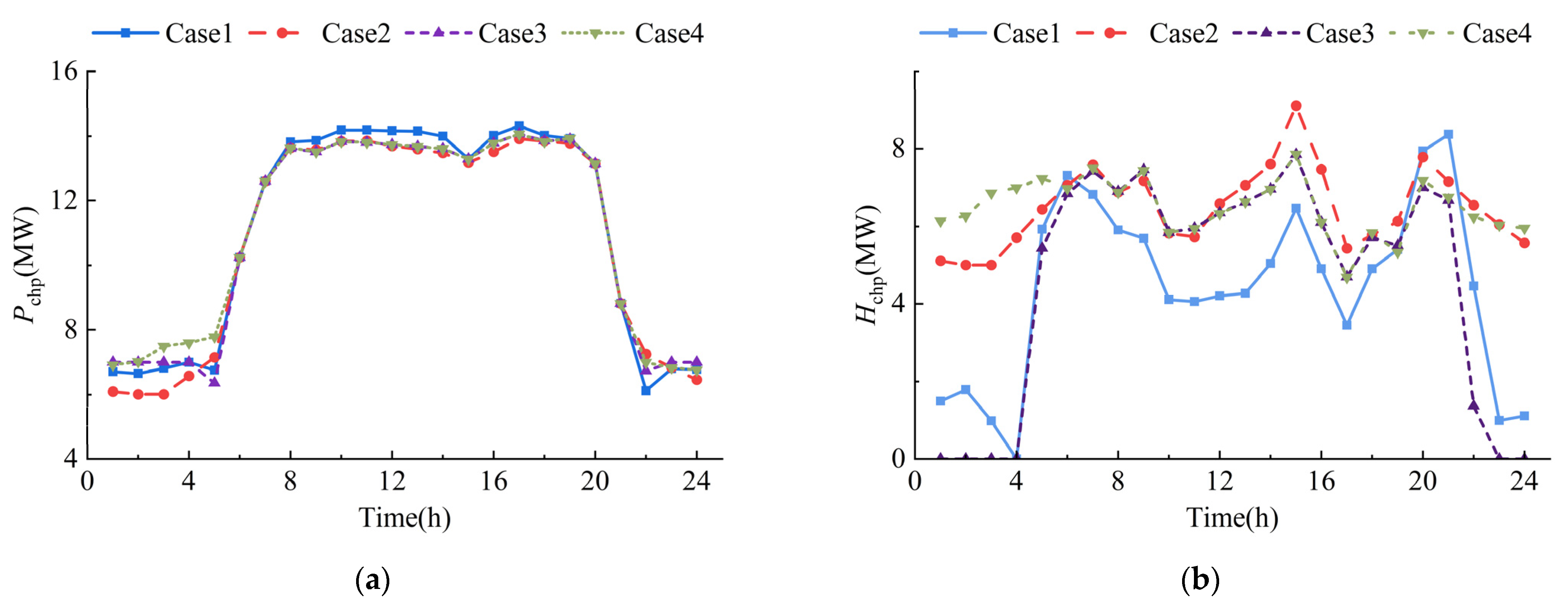
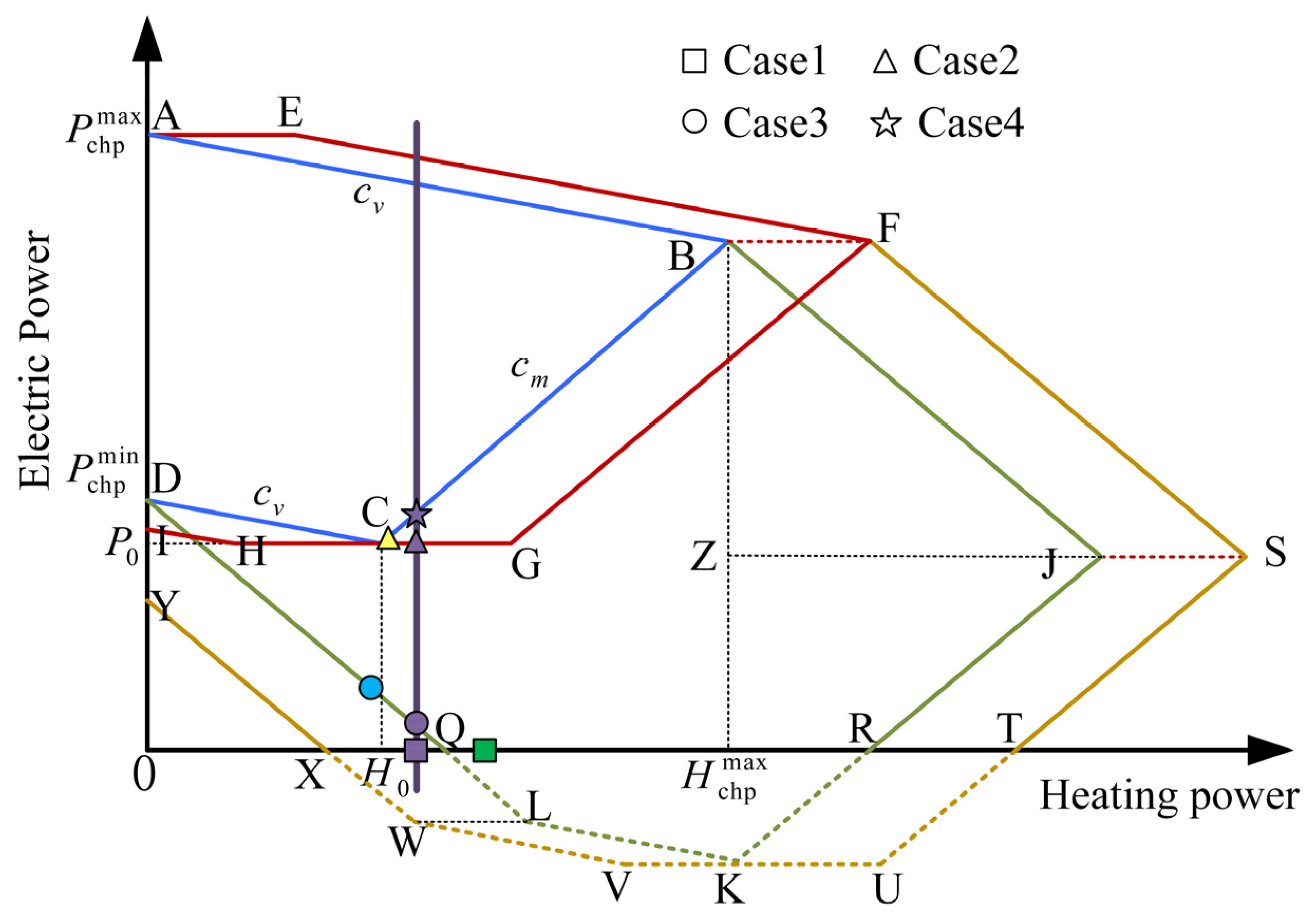
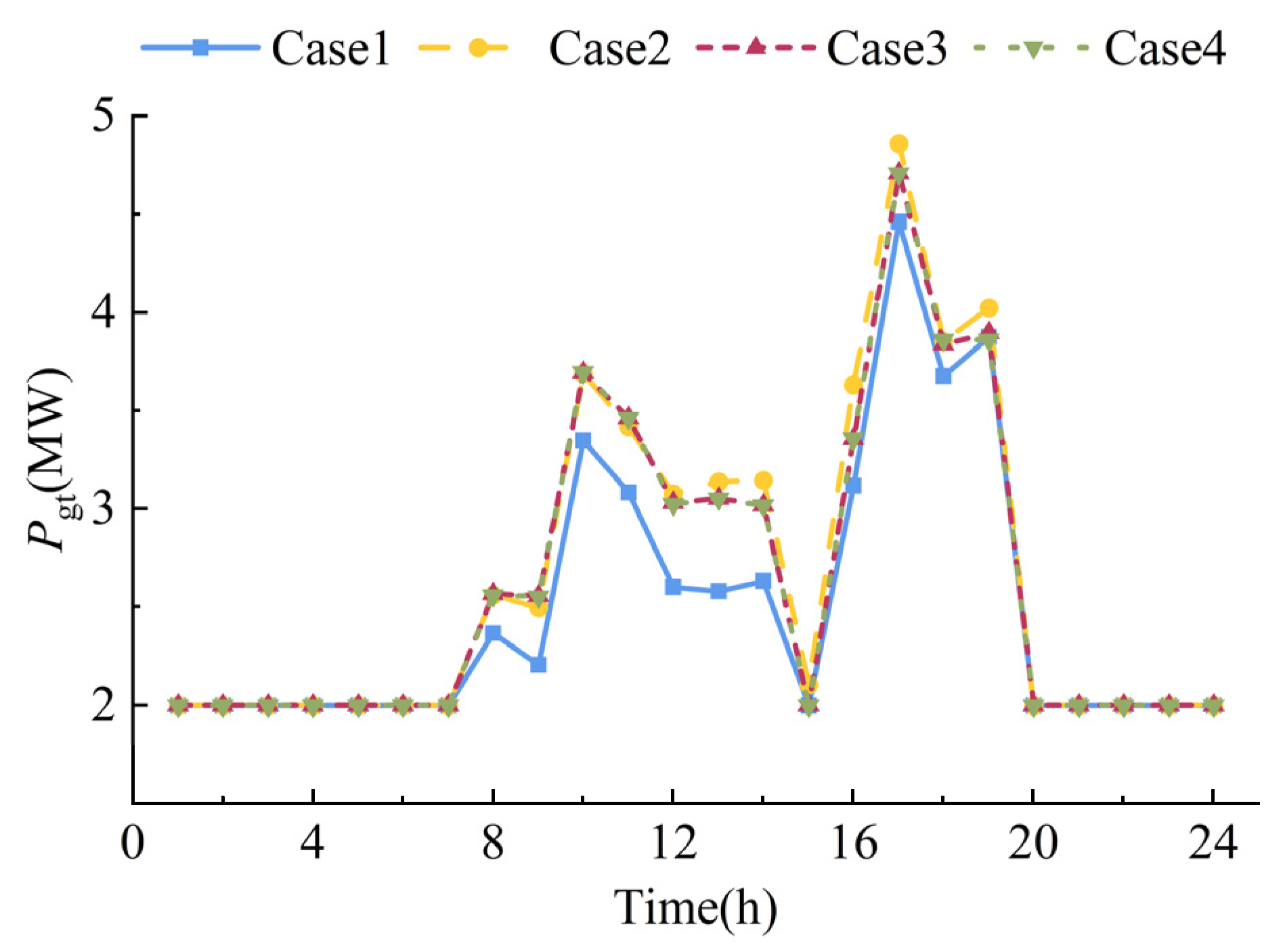
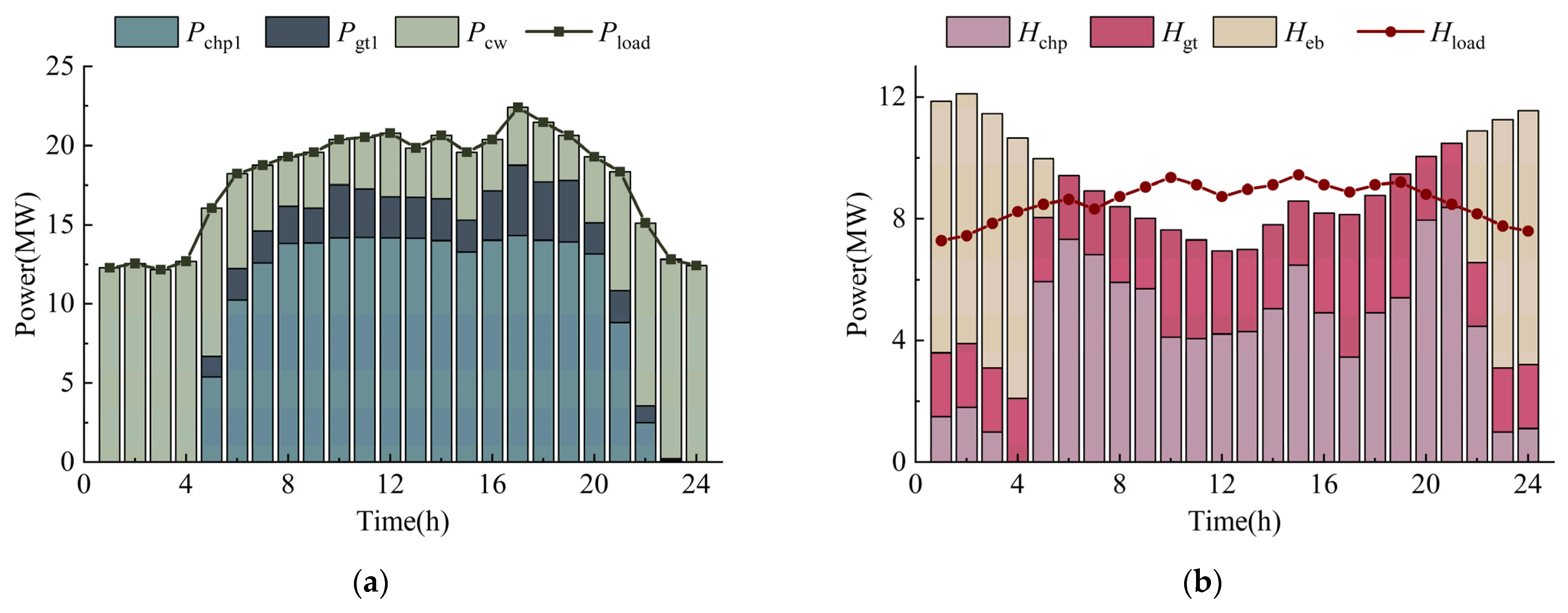
4.3. Comparison of Equipment Outputs under Different Dispatch Cases

The electrical power output of the CHP under four cases is compared in Figure 8a, while the heat power output of CHP is compared in Figure 8b. From the figures, it can be observed that the electricity output of the CHP was lower during 0:00–5:00 and 21:00–24:00 compared with the other periods. This reduction was attributed to the higher WT output during these periods, which resulted in the lowering of electricity output from the CHP to increase wind power consumption and improve the overall economy of the operation of the system.

Comparing case 2 and case 4 from 0:00 to 5:00, the electric and thermal outputs of CHP in case 2 are both reduced relative to case 4. This reduction was due to the exothermic heat release of the pipe network in this period, which reduces the thermal output of the CHP, and consequently, the electric output of CHP could be reduced accordingly. However, in case 4, the electric output of the CHP could not be reduced due to the constraints of the thermal output. In case 2, the CHP increased the heat output during 13:00–16:00 and 20:00–22:00, while the pipe network was in heat storage during these periods. When comparing case 3 and case 4, during the periods of 22:00–24:00 and 0:00–4:00, in case 3, the CHP did not emit thermal power, and it operated at the minimum electrical output in the pure condensation state. This was due to the conversion of the forced electrical power of the CHP to thermal output through the EB in order to increase the wind power consumption. In the 4:00–5:00 period, the WT output decreased relative to 0:00–4:00, and reducing the output of the EB could consume all the wind power, leading to the need for the CHP to increase the thermal output, making the electric output of the CHP decrease accordingly. When comparing case 1 and case 4, in case 4, the electric output of the CHP was smaller when the WT output was rich and increased during other periods. This was due to the fact that the heat release from the heating network could increase the electric output of the CHP by reducing its heat output during hours of higher electric load demand. When comparing case 1 and case 3 during the periods of 22:00–24:00 and 0:00–3:00, it is evident that the thermal output of the CHP was higher in case 1. This discrepancy arose from the heat release occurring within the heating network from 9:00 to 17:00, which could reduce the power output of the GT. Due to the superior cost efficiency of the CHP, its heat output was intentionally increased during 22:00–24:00 and 0:00–3:00 to enhance the heat storage in the network.

Figure 9 provides a deeper analysis of the operational characteristics of the CHP system, taking into account heat storage within the heating network and the configuration of the EB. In this figure, the operational range of the CHP itself, as well as the range when considering only heating network heat storage, remained consistent with that depicted in Figure 4. However, the scenario changed when focusing solely on the EB, resulting in an operational range of ABJRQD. This shift was attributable to the larger capacity of the EB, exceeding the minimum required forced electric power output of the CHP. When both the EB and heating network heat storage were factored in, the combined external operational range emerged as AEFSTXY. The length of BZ signified Pmax gt. The period from 0:00 to 1:00 was selected for analysis. Since case 4 did not consider heating network heat storage and the EB, the CHP output from this case served as the benchmark for comparison, as represented by the purple pentagon in the figure. In case 2, only the heating network heat storage was taken into consideration. The forced electric power of the CHP sent to the grid could be reduced, at most, to match the value corresponding to the purple triangle. This reduction aimed to increase wind power consumption. The CHP’s actual operational position is symbolized by the yellow triangle. The difference in horizontal coordinates between these two triangles signifies the heat release power of the heating network. In case 3, only the EB was taken into consideration. The forced electric power conveyed from the CHP to the grid could be decreased down to the value corresponding to the purple circle, with the intention of enhancing wind power consumption. However, the further increase in the EB output was restrained by the constraints of the thermal load demand. The overall external operational position of the CHP, when considering the EB, is depicted by the blue circle. This positioning arose because, between 0:00 and 1:00, a portion of the forced electric power generated by the GT was converted into thermal power. Due to an unchanged thermal demand, the electric power input from the CHP to the EB diminished in comparison with the level indicated by the purple circle. In case 1, both the heating network heat storage and the EB were taken into account. The forced electric power transmitted from the CHP to the grid could be reduced down to the value corresponding to the purple square, at most. In contrast with scenarios where only the EB was taken into consideration, the output of the EB was no longer constrained by the heat load demand in this case. As a result, a greater amount of the forced electric power generated by the CHP could be converted into heat power. The actual operational position of case 1 corresponds to the green square, and the discrepancy between the horizontal coordinates of these two squares represents the exothermic power of the heating network during this period.

The comparison of the electrical output of GT in four different cases is depicted in Figure 10. The thermal output of GT was directly proportional to its electrical output. In both case 3 and case 4, the GT was operated at the minimum output allowed for the safe operation of the system and itself, owing to its higher operating cost compared with the CHP. Only after the CHP had fully generated its output, the GT output was increased to meet the load demand. In case 2, the output of GT increased during three specific periods: 12:00–14:00, 15:00–17:00, and 18:00–19:00. This increase is attributed to the need for the heating network to store heat, resulting in a rise in the heat output of the CHP. Consequently, the electrical output of the CHP decreased, requiring the GT output to be increased during these periods to meet the electrical load demand. In case 1, from 7:00 to 19:00, the heating network operated in a heat-release state, leading to a decrease in the heat output of the CHP. This decrease allowed for an increase in the electrical output of the CHP. Considering the superior economic efficiency of the CHP compared with the GT, the output of the GT was intentionally reduced during this period to enhance the overall economy of the system operation.

4.4. Comparison of the Economics and Wind Integration under Different Dispatch Cases

The operating cost of the system and the percentage of wind power consumption in the four cases are compared in

Table 5. Operating costs of the system and percentage of wind power consumption with four cases.

Case	Operating Costs (USD)	Percentage of Wind Power Consumption (%)
Case 1	9152.0	96.89%
Case 2	9908.0	61.67%
Case 3	9459.2	89.04%
Case 4	9967.8	58.59%

. The wind power consumption in the four cases is illustrated in Figure 11 and Figure 12a,b, which depict the heat storage in the heating network in case 2 and case 1, respectively. From the analysis of Table 5 and Figure 11, it became evident that higher wind power consumption led to lower system operating costs. This outcome can be attributed to two factors. First, increased wind power consumption reduced the output of both the CHP and GT, resulting in lower operating costs for them. Second, higher wind power consumption reduced the penalty costs associated with wind abandonment.

In case 2, the rise in wind power consumption was facilitated by the regulating effect of the HSHN, as shown in Figure 12a. During the period from 0:00 to 5:00, the heating network released heat, leading to reduced heat output of the CHP and subsequently lower electricity output. This allowed the system to consume more wind power during this time. However, it should be noted that the cost reduction was only about 0.6% when considering only the HSHN. This was because there was a considerable amount of forced electric power in the CHP and GT, and lowering their heat output had a limited impact on their electric power output connected to the grid, thus affecting the wind power consumption. In case 3, the increase in wind power consumption was attributed to the configuration of the EB, which converted a portion of the forced electric power from the CHP and GT into thermal power. This conversion not only freed up space for wind power consumption by reducing their electric power output but it also reduced the thermal output of the CHP. Compared with case 2, the configuration of the EB significantly enhanced the wind power consumption, leading to an improved system operating economy of about 5.1%. In case 1, the enhanced wind power consumption resulted from a combination of the HSHN and EB. This enabled the CHP and GT to achieve further thermo-electrolytic decoupled operation. The operating cost of the system was reduced by about 8.2%, which was more economical than the sum of considering the HSHN and EB separately. The key reason behind this was that during times of high wind power output, the output of the EB was no longer constrained by the heat load demand compared with case 3. It allowed for a further increase in the output of the EB, which reduced the electric output supplied by the CHP and GT to the grid, leading to greater wind power consumption. Simultaneously, excess heat energy was stored in the heating network, as depicted in Figure 12b. During times of high electric load demand, the heat released from the pipe network decreased the heat output of CHP while increasing its electric output, also resulting in a reduction in GT output and further lowering the operating cost of the system.

4.5. Further Analysis with Power Balance

To further analyze the impact of the HSHN and EB on the system operation, the power balances of case 1 and case 3 were compared. The thermal power balance of case 3 is depicted in Figure 13b, revealing that the period of highest heat load demand does not align with the period of highest heat energy supply. This indicates a significant transmission delay in the thermal system. Additionally, it can be observed that the thermal energy transmission process incurred an energy loss of about 9.5%. When only the EB was considered during times of high wind power output, the EB output was constrained by the thermal load demand, allowing for only a portion of the forced electric power from the CHP and GT to be converted to thermal power through the EB, as shown in Figure 13a. However, when the regulating effect of heat storage in the pipe network was considered, the thermal load demand constraint was broken. Consequently, all of the forced power from the CHP and GT could be converted into thermal power through the EB, further enhancing the wind power consumption capability, as depicted in Figure 14a. In case 1, the upper limit of the wind power consumption capability depended on the thermal network constraints and equipment output constraints.

In times of high electric load demand, the wind power output was low, and priority was given to increasing the output of the more economical CHP until it reached its maximum capacity. As shown in Figure 14b, the pipe network released heat when the CHP was operating at its full capacity, resulting in a decrease in the thermal output of the CHP and enabling an increase in its electrical output. Consequently, the output of the GT could be reduced to lower the overall system operating cost. During 21:00–22:00, all wind power could be consumed by considering only the EB. At this time, the system performed thermal storage in the pipe network, and the most economical approach was to reduce the power output of CHP and increase its heat output.

5. Conclusions

In this paper, the fictitious node method is introduced as a novel method for calculating quasi-dynamic processes in the thermal system, with the aim to achieve more effective coordinated scheduling of electric and thermal systems. Unlike traditional approaches, this method offers a specific calculation time; as such, the computational accuracy of this method is not dependent on the scheduling interval but rather closely associated with the computation time. Simulation experiments demonstrated that the method offered certain advantages in terms of calculation accuracy and complexity. Leveraging the capabilities of the fictitious node method in providing efficient computational information, a methodology for quantifying the heat storage capacity of the heating pipeline network is proposed. Moreover, this study investigated the influence of heat storage in the heating network on system operation. The proposed strategy encompasses the conversion of a portion of the forced electrical power generated by CHP units and gas turbine units into thermal energy through electric boilers, which is then efficiently stored using the heating network’s heat storage capacity. Simulation experiments further validated that the comprehensive consideration of heat storage within the pipeline network, coupled with an EB configuration, significantly amplified wind power integration and consumption capacity while simultaneously curbing energy production costs. The optimal configuration presented in this paper resulted in an 8.2% enhancement in system operating economics and an impressive 38.3% increase in wind power integration.

For future research, the role of heat storage in the pipeline network in the system’s multi-time scale scheduling is planned to be explored. Furthermore, investigating the interaction between heat storage in the pipeline network and other influencing factors in system operation is on the agenda. The detailed modeling of equipment and systems is also identified as a crucial and intriguing area of study that should not be overlooked.

References

1. Global Wind Energy Council (GWEC). Global Wind Report 2023. Available online: https://gwec.net/globalwindreport2023/ (accessed on 23 August 2023).
2. Sayed, E.T.; Rezk, H.; Olabi, A.G.; Gomaa, M.R.; Hassan, Y.B.; Rahman, S.M.A.; Shah, S.K.; Abdelkareem, M.A. Application of Artificial Intelligence to Improve the Thermal Energy and Exergy of Nanofluid-Based PV Thermal/Nano-Enhanced Phase Change Material. Energies 2022, 15, 8494. [Google Scholar] [CrossRef]
3. Al-Rawashdeh, H.; Al-Khashman, O.A.; Al Bdour, J.T.; Gomaa, M.R.; Rezk, H.; Marashli, A.; Arrfou, L.M.; Louzazni, M. Performance Analysis of a Hybrid Renewable-Energy System for Green Buildings to Improve Efficiency and Reduce GHG Emissions with Multiple Scenarios. Sustainability 2023, 15, 7529. [Google Scholar] [CrossRef]
4. Al-Rawashdeh, H.; Al-Khashman, O.A.; Arrfou, L.M.; Gomaa, M.; Rezk, H.; Shalby, M.; Al Bdour, J.; Louzazni, M. Different Scenarios for Reducing Carbon Emissions, Optimal Sizing, and Design of a Stand-Alone Hybrid Renewable Energy System for Irrigation Purposes. Int. J. Energy Res. 2023, 2023, 6338448. [Google Scholar] [CrossRef]
5. Gomaa, M.R.; Ala’a, K.; Al-Dhaifallah, M.; Rezk, H.; Ahmed, M. Optimal design and economic analysis of a hybrid renewable energy system for powering and desalinating seawater. Energy Rep. 2023, 9, 2473–2493. [Google Scholar] [CrossRef]
6. Pan, Z.; Guo, Q.; Sun, H. Interactions of district electricity and heating systems considering time-scale characteristics based on quasi-steady multi-energy flow. Appl. Energy 2016, 167, 230–243. [Google Scholar] [CrossRef]
7. Liu, X.; Wu, J.; Jenkins, N.; Bagdanavicius, A. Combined analysis of electricity and heat networks. Appl. Energy 2016, 162, 1238–1250. [Google Scholar] [CrossRef]
8. Jiang, X.S.; Jing, Z.X.; Li, Y.Z.; Wu, Q.H. Modelling and operation optimization of an integrated energy based direct district water-heating system. Energy 2014, 64, 375–388. [Google Scholar] [CrossRef]
9. Li, J.; Fang, J.; Zeng, Q.; Chen, Z. Optimal operation of the integrated electrical and heating systems to accommodate the intermittent renewable sources. Appl. Energy 2016, 167, 244–254. [Google Scholar] [CrossRef]
10. Pan, Z.; Wu, J.; Sun, H.; Guo, Q.; Abeysekera, M. Quasi-dynamic interactions and security control of integrated electricity and heating systems in normal operations. CSEE J. Power Energy Syst. 2019, 5, 120–129. [Google Scholar] [CrossRef]
11. Li, X.; Li, W.; Zhang, R.; Jiang, T.; Chen, H.; Li, G. Collaborative scheduling and flexibility assessment of integrated electricity and district heating systems utilizing thermal inertia of district heating network and aggregated buildings. Appl. Energy 2020, 258, 114021. [Google Scholar] [CrossRef]
12. Turski, M.; Sekret, R. Buildings and a district heating network as thermal energy storages in the district heating system. Energy Build. 2018, 179, 49–56. [Google Scholar] [CrossRef]
13. Xu, X.; Lyu, Q.; Qadrdan, M.; Wu, J. Quantification of Flexibility of a District Heating System for the Power Grid. IEEE Trans. Sustain. Energy 2020, 11, 2617–2630. [Google Scholar] [CrossRef]
14. Dai, Y.; Chen, L.; Min, Y.; Chen, Q.; Hao, J.; Hu, K. Dispatch Model for CHP With Pipeline and Building Thermal Energy Storage Considering Heat Transfer Process. IEEE Trans. Sustain. Energy 2019, 10, 192–203. [Google Scholar] [CrossRef]
15. Wu, C.; Gu, W.; Jiang, P.; Li, Z.; Li, B. Combined Economic Dispatch Considering the Time-Delay of District Heating Network and Multi-Regional Indoor Temperature Control. IEEE Trans. Sustain. Energy 2018, 9, 118–127. [Google Scholar] [CrossRef]
16. Gu, W.; Wang, J.; Lu, S.; Luo, Z.; Wu, C. Optimal operation for integrated energy system considering thermal inertia of district heating network and buildings. Appl. Energy 2017, 199, 234–246. [Google Scholar] [CrossRef]
17. Wei, W.; Wu, J.; Mu, Y.; Wu, J.; Jia, H.; Yuan, K.; Song, Y.; Sun, C. Assessment of the solar energy accommodation capability of the district integrated energy systems considering the transmission delay of the heating network. Int. J. Electric. Power Energy Syst. 2021, 130, 106821. [Google Scholar] [CrossRef]
18. Wu, S.; Li, H.; Liu, Y.; Lu, Y.; Wang, Z.; Liu, Y. A two-stage rolling optimization strategy for park-level integrated energy system considering multi-energy flexibility. Int. J. Electric. Power Energy Syst. 2023, 145, 108600. [Google Scholar] [CrossRef]
19. Zhou, S.J.; Tian, M.C.; Zhao, Y.E.; Guo, M. Dynamic modeling of thermal conditions for hot-water district-heating networks. J. Hydrodyn. 2014, 26, 531–537. [Google Scholar] [CrossRef]
20. Wang, Y.; You, S.; Zhang, H.; Zheng, X.; Zheng, W.; Miao, Q.; Lu, G. Thermal transient prediction of district heating pipeline: Optimal selection of the time and spatial steps for fast and accurate calculation. Appl. Energy 2017, 206, 900–910. [Google Scholar] [CrossRef]
21. Tang, Z.; Lin, S.; Liang, W.; Xie, Y.; Liu, M. Optimal Dispatch of Integrated Energy Campus Microgrids Considering the Time-Delay of Pipelines. IEEE Access 2020, 8, 178782–178795. [Google Scholar] [CrossRef]
22. Lu, S.; Gu, W.; Zhou, S.; Yu, W.; Pan, G. High-Resolution Modeling and Decentralized Dispatch of Heat and Electricity Integrated Energy System. IEEE Trans. Sustain. Energy 2020, 11, 1451–1463. [Google Scholar] [CrossRef]
23. Li, Z.; Wu, W.; Shahidehpour, M.; Wang, J.; Zhang, B. Combined Heat and Power Dispatch Considering Pipeline Energy Storage of District Heating Network. IEEE Trans. Sustain. Energy 2016, 7, 12–22. [Google Scholar] [CrossRef]
24. Li, Z.; Wu, W.; Wang, J.; Zhang, B.; Zheng, T. Transmission-Constrained Unit Commitment Considering Combined Electricity and District Heating Networks. IEEE Trans. Sustain. Energy 2016, 7, 480–492. [Google Scholar] [CrossRef]
25. Liu, X.; Hou, M.; Sun, S.; Wang, J.; Sun, Q.; Dong, C. Multi-time scale optimal scheduling of integrated electricity and district heating systems considering thermal comfort of users: An enhanced-interval optimization method. Energy 2022, 145, 124311. [Google Scholar] [CrossRef]
26. Huang, J.; Li, Z.; Wu, Q. Coordinated dispatch of electric power and district heating networks: A decentralized solution using optimality condition decomposition. Appl. Energy 2017, 206, 1508–1522. [Google Scholar] [CrossRef]
27. Jiang, Y.; Wan, C.; Botterud, A.; Song, Y.; Xia, S. Exploiting Flexibility of District Heating Networks in Combined Heat and Power Dispatch. IEEE Trans. Sustain. Energy 2020, 11, 2174–2188. [Google Scholar] [CrossRef]
28. Chen, Y.; Guo, Q.; Sun, H.; Li, Z.; Pan, Z.; Wu, W. A water mass method and its application to integrated heat and electricity dispatch considering thermal inertias. Energy 2019, 181, 840–852. [Google Scholar] [CrossRef]
29. Lu, S.; Gu, W.; Zhang, C.; Meng, K.; Dong, Z. Hydraulic-Thermal Cooperative Optimization of Integrated Energy Systems: A Convex Optimization Approach. IEEE Trans. Smart Grid. 2020, 11, 4818–4832. [Google Scholar] [CrossRef]
30. Lu, S.; Gu, W.; Meng, K.; Yao, S.; Liu, B.; Dong, Z. Thermal Inertial Aggregation Model for Integrated Energy Systems. IEEE Trans. Power Syst. 2020, 35, 2374–2387. [Google Scholar] [CrossRef]
31. Hao, J.; Chen, Q.; He, K.; Chen, L.; Dai, Y.; Xu, F.; Min, Y. A Heat Current Model for Heat Transfer/Storage Systems and Its Application in Integrated Analysis and Optimization with Power Systems. IEEE Trans. Sustain. Energy 2020, 11, 175–184. [Google Scholar] [CrossRef]
32. Xu, F.; Hao, L.; Chen, L.; Chen, Q.; Wei, M.; Min, Y. Integrated heat and power optimal dispatch method considering the district heating networks flow rate regulation for wind power accommodation. Energy 2023, 263, 125656. [Google Scholar] [CrossRef]
33. Gou, X.; Chen, Q.; He, K. Real-time quantification for dynamic heat storage characteristic of district heating system and its application in dispatch of integrated energy system. Energy 2022, 259, 124960. [Google Scholar] [CrossRef]
34. Sun, Q.; Zhao, T.; Chen, Q.; He, K.; Ma, H. Decentralized Dispatch of Distributed Multi-Energy Systems with Comprehensive Regulation of Heat Transport in District Heating Networks. IEEE Trans. Sustain. Energy 2023, 14, 97–110. [Google Scholar] [CrossRef]
35. Nuytten, T.; Claessens, B.; Paredis, K.; Bael, J.V.; Six, D. Flexibility of a combined heat and power system with thermal energy storage for district heating. Appl. Energy 2013, 104, 583–591. [Google Scholar] [CrossRef]
36. Chen, X.; Kang, C.; O’Malley, M.; Xia, Q.; Bai, J.; Liu, C.; Sun, R.; Wang, W.; Li, H. Increasing the Flexibility of Combined Heat and Power for Wind Power Integration in China: Modeling and Implications. IEEE Trans. Power Syst. 2015, 30, 1848–1857. [Google Scholar] [CrossRef]
37. Li, Y.; Wang, C.; Li, G.; Wang, J.; Zhao, D.; Chen, C. Improving operational flexibility of integrated energy system with uncertain renewable generations considering thermal inertia of buildings. Energy Convers. Manag. 2020, 207, 112526. [Google Scholar] [CrossRef]
38. Dai, Y.; Chen, L.; Min, Y.; Mancarella, P.; Chen, Q.; Hao, J.; Kang, H.; Fei, X. Integrated Dispatch Model for Combined Heat and Power Plant with Phase-Change Thermal Energy Storage Considering Heat Transfer Process. IEEE Trans. Sustain. Energy 2018, 9, 1234–1243. [Google Scholar] [CrossRef]
39. Zhu, M.; Li, J. Integrated dispatch for combined heat and power with thermal energy storage considering heat transfer delay. Energy 2022, 244, 123230. [Google Scholar] [CrossRef]
40. Xue, Y.; Shahidehpour, M.; Pan, Z.; Wang, B.; Zhou, Q.; Guo, Q.; Sun, H. Reconfiguration of District Heating Network for Operational Flexibility Enhancement in Power System Unit Commitment. IEEE Trans. Sustain. Energy 2021, 12, 1161–1173. [Google Scholar] [CrossRef]
41. Ma, Y.; Wang, H.; Hong, F.; Yang, J.; Feng, J. Modeling and optimization of combined heat and power with power-to-gas and carbon capture system in integrated energy system. Energy 2021, 236, 121392. [Google Scholar] [CrossRef]
42. Li, J.; Lin, J.; Song, Y.; Xing, X.; Fu, C. Operation Optimization of Power to Hydrogen and Heat (P2HH) in ADN Coordinated with the District Heating Network. IEEE Trans. Sustain. Energy 2019, 10, 1672–1683. [Google Scholar] [CrossRef]
43. Wang, D.; Zhi, Y.Q.; Jia, H.J.; Hou, K.; Zhang, S.; Du, W.; Fan, M. Optimal scheduling strategy of district integrated heat and power system with wind power and multiple energy stations considering thermal inertia of buildings under different heating regulation modes. Appl. Energy 2019, 240, 341–358. [Google Scholar] [CrossRef]
44. Wang, J.; Huo, S.; Yan, R.; Cui, Z. Leveraging heat accumulation of district heating network to improve performances of integrated energy system under source-load uncertainties. Energy 2022, 252, 124002. [Google Scholar] [CrossRef]
45. Ministry of Housing and Urban-Rural Development of the People’s Republic of China. Technical Specification for Directly Buried Hot-Water Heating Pipeline in City: CJJ/T 81—2013; China Architecture and Building Press: Beijing, China, 2013. (In Chinese) [Google Scholar]
46. Fan, A.; Liu, W.; Wang, C. Simulation on the daily change of soil temperature under various environment conditions. Acta Energ. Sol. Sin. 2003, 4, 167–171. (In Chinese) [Google Scholar]
47. Wang, N. Numerical Methods and Dynamic Characteristic Analysis of the Thermal and Hydraulic Transients in District Heating Network. Ph.D. Thesis, Tianjin University, Tianjin, China, 2019. [Google Scholar]
Figure 1. Thermal flow model of the primary network.
Energies 16 06449 g001
Figure 2. The 6-node heating network and the description of fictitious node method.
Energies 16 06449 g002
Figure 3. Structure of the electricity and heat integrated energy system.
Energies 16 06449 g003
Figure 4. Operating characteristics of CHP.
Energies 16 06449 g004
Figure 5. The 27-node heating network.
Energies 16 06449 g005
Figure 6. Load demand and wind power forecasting curves.
Energies 16 06449 g006
Figure 7. (a) Scheduling results of the output of heat sources in case 3; (b) comparison of the two Tr,out in case 1.
Energies 16 06449 g007
Figure 8. (a) Comparison of the electrical power output of the CHP in four cases; (b) comparison of the heat power output of CHP in four cases.
Energies 16 06449 g008
Figure 9. Comparison of the external operation of CHP in four cases.
Energies 16 06449 g009
Figure 10. Comparison of the electrical output of GT in four cases.
Energies 16 06449 g010
Figure 11. Comparison of wind power consumption in four cases.
Energies 16 06449 g011
Figure 12. (a) Heat storage in heating network of case 2; (b) heat storage in heating network of case 1.
Energies 16 06449 g012
Figure 13. (a) Electrical power balance in case 3; (b) heat power balance in case 3.
Energies 16 06449 g013
Figure 14. (a) Electrical power balance in case 1; (b) heat power balance in case 1.
Energies 16 06449 g014