Zero-Carbon AC/DC Microgrid Planning by Leveraging Vehicle-to-Grid Technologies

Abstract

This paper explores the strategic planning required for a zero-carbon-emission AC/DC microgrid, which integrates renewable energy sources and electric vehicles (EVs) within its framework. It considers the rapidly growing adoption of EVs and the advent of vehicle-to-grid (V2G) technology, which allows EVs to return energy to the grid during peak demand. The study aims to apply optimization techniques to minimize the installation cost associated with various microgrid components. In the case of microgrids, there are decision-making scenarios where multiple alternatives are present; optimization is a valuable technique for efficiently planning and designing microgrids. This work showcases case studies and sensitivity analysis plots, illustrating how output power fluctuates due to uncertainty in renewable energy sources and the absence of EVs. The findings show how V2G contributes to the demand when renewable generation is low. The sensitivity analysis also provides insights into how the unit cost is affected by demand fluctuations. In summary, the principal contribution of this study is developing a comprehensive planning framework for AC/DC microgrids. This framework considers the escalating adoption of EVs and offers practical solutions for future microgrid designs.

1. Introduction

Electricity is a critical component of modern life, serving as the cornerstone for industrialization, urbanization, economic growth, and societal quality of life improvement [1]. It plays a vital role in various aspects of our daily lives, powering a multitude of entities such as computers, machinery, public transport, home appliances, and healthcare services. Yet, it is important to recognize that despite its widespread usage, there are still regions worldwide where electricity is either scarce or entirely unavailable. This omnipresent electricity is delivered through a network known as the electric grid.

The power grid is a complex infrastructure designed for the generation, transmission, and distribution of electricity. It functions as an interconnected network that facilitates the delivery of electricity from suppliers to consumers. The conventional grid operates traditionally where energy is generated at a central power plant and transmitted and distributed over considerable distances. This system consists of generating units, high-voltage transmission lines, substations, and transformers for adjusting voltage levels. The conventional grids are evaluated on their reliability, efficiency, and cost-effectiveness. However, due to the substantial distance between power sources and load centers, transmission losses are practically unavoidable. Grid faults can result in total power outages, and the use of traditional fossil fuels, which serve as the main source of power generation, contributes to environmental pollution and global warming. Moreover, any disruption at the substation, the intermediary between the power plant and the customer, results in a power loss for the customer.

To address these issues, decentralized power generation units, commonly known as microgrids, have been developed. A microgrid is an independent energy generation unit comprising renewable energy sources and power converters. Microgrids can provide energy during primary grid power failures or peak demand. They can also operate independently, supplying power to a small area, community, or industry. The primary advantage of a microgrid is its ability to incorporate various energy generation methods, particularly renewable energy sources. The size of a microgrid typically ranges from 100 KW to several Megawatts, and these are highly flexible, efficient, and cost-effective energy grids [2]. A microgrid comprises renewable generating units such as photovoltaic (PV) cells, wind units, and natural gas, which are abundant, environmentally friendly, and more sustainable compared to fossil fuels. Synchronizing with the main power grid can be challenging, but the process can be made more efficient using distributed generators. Depending on the community’s power demands, energy storage in batteries may be required [2]. A microgrid can significantly reduce transmission and distribution losses, thus saving wasted electricity.

With the increasing population and industrialization, the need for transportation has risen. Traditional vehicles have been the standard means of transportation, but they come with drawbacks such as high fuel costs and environmental pollution. The limited availability of fossil fuels is another concern. A promising solution to mitigate these challenges is the introduction of electric vehicles (EVs). An increase in the number of EVs has sparked a revolution in the transportation and energy sectors. EV technology utilizes electricity to power an electric motor instead of an internal combustion engine, resulting in zero carbon emissions. EVs are powered by lithium-ion batteries, which act as energy storage devices. This capability can be leveraged as an additional energy source for industrial or household demand as the increasing number of EVs on the road augments this storage capacity, significantly impacting the broader energy sector. Microgrids can supply power for EV charging, and when EVs are idle, they can serve as energy storage units for the microgrid during peak hours or power outages. This bidirectional energy exchange is called vehicle-to-grid (V2G) technology. Hence, EVs equipped with V2G capabilities are becoming reliable and flexible resources for energy balancing under varying energy supply and demand scenarios [3]. EVs can balance load by managing their charging and discharging cycles based on electricity demand. Consequently, integrating EVs into microgrids satisfies transportation needs and offers a sophisticated approach to energy management and distribution.

This section is structured as follows: Section 1.1 introduces the optimization concept and discusses its efficacy in microgrid planning. Section 1.2 examines previous studies on optimization techniques, zero-carbon-emission microgrids, AC/DC microgrid planning, EV integration in a microgrid, and the benefits of using the Julia programming language to solve optimization problems. Section 1.3 addresses the existing challenges in power distribution systems and the benefits of utilizing a zero-carbon-emission AC/DC microgrid to formulate a problem statement. It also outlines the significant role EVs play in supporting energy management within the microgrid. Section 1.4 describes the solution to the planning problem, giving an overview of the system and system parameters. It also briefly discusses the optimization technique and software used to derive the desired solution. Lastly, Section 2 and Section 2.1 introduce the microgrid architecture, i.e., network topology and the significance of grid elements considered in the system for the next ten years of microgrid planning.

1.1. Role of Optimization in Microgrid Planning

Optimization is a process that aims to pinpoint the optimal solution or set of solutions based on a given set of constraints and objectives. It is a versatile tool utilized in diverse fields such as engineering, economics, finance, and computer science. Its application is particularly valuable in decision-making scenarios where multiple alternatives are present, and resources are limited.

Optimization problems can vary greatly, ranging from linear or nonlinear to continuous or discrete, and from deterministic to stochastic. A broad array of techniques is used to solve these problems, including but not limited to linear programming, quadratic programming, nonlinear programming, and dynamic programming. These techniques harness the power of mathematical algorithms and computational methodologies to discover optimal solutions.

In the microgrid context, optimization plays a crucial role in resource planning. As a multifaceted system, a microgrid integrates several energy generation units such as solar units, wind turbines, and energy storage systems such as batteries in EVs. Moreover, transmission lines and converters, alongside varying installation, maintenance costs, and capacities, add layers of complexity to the microgrid planning process. The wide range of variables and their respective constraints make microgrid resource utilization highly multi-factorial. In previous work [4], optimization techniques for planning of a hybrid AC/DC microgrid were studied by using different algorithms. A genetic algorithm was proposed for optimal sizing and a nonlinear solver was deployed to solve the operational problem subject to the obtained design/investment decisions.

Integrating EVs into the microgrid introduces another dimension to the optimization problem. With their charging and discharging schedules, EVs can significantly influence electricity costs, grid reliability, and the utilization rate of renewable energy. Considerations such as EVs’ significance, battery capacity, travel patterns, and charging preferences further complicate the situation. In light of these complexities, optimization presents a systematic approach to designing and planning a microgrid. It facilitates decisions regarding unit installation over the next decade, taking into account the various complexities and uncertainties inherent in the model.

1.2. Literature Review

This section provides a concise overview of previous studies and approaches in microgrid planning, offering a comprehensive literature review covering various subjects. This includes studies on zero-carbon microgrids, hybrid AC/DC microgrids, and integrating electric vehicles into the microgrid. It also sheds light on different optimization techniques used in microgrid planning.

A notable study [5] examined provisional microgrid planning, paying special attention to various uncertainties in the planning process. These uncertainties include variable market prices, diverse renewable generation output, load errors, and islanding uncertainty—the capacity of a microgrid to operate autonomously and independently in the event of power outages. The study developed a model to determine the most cost-effective installation of renewable distribution energy sources, maximizing the objective over uncertainty sets to achieve the worst-case microgrid optimal operation solution. It employed robust optimization to efficiently account for physical and financial uncertainties [5]. The approach for considering uncertainties in renewable generation and total load from this paper was adopted in the current work to derive more realistic solutions.

Another noteworthy study [6] tackled multi-objective energy management in microgrids. The research presented a microgrid with hybrid energy sources, including renewable and fossil fuel sources, and a battery energy storage system. The study’s objectives involved minimizing operating costs, power loss, and greenhouse gas emissions, demonstrating a potential reduction in CO₂ emissions by 51.6 percent compared to traditional grids powered by fossil fuel energy sources. This study was referenced in the current work, and its approach to using electric vehicles for energy storage was incorporated. However, in contrast to the study’s hybrid sources, this paper opts for exclusively utilizing renewable energy sources, thereby achieving zero carbon emissions.

Article [7] delivered a detailed overview of the role played by different optimization techniques in energy management within a microgrid. It elaborated on factors such as forecasting, demand management, and economic dispatch that govern the choice of optimization technique. The article discussed the fuzzy-logic-based optimization technique, which utilizes fuzzy rules and logical segments to optimize the energy storage system’s operational costs and battery life in a microgrid. Furthermore, it highlighted the multi-agent-based technique that effectively coordinates renewable energy sources and demand response, as well as the neural-network-based technique employed for load response planning, economic dispatch, and the optimal operation of renewable energy integration [7]. In contrast, the current work applies the mixed-integer programming-based technique, a conventional method known for its computational efficiency in managing energy generation, demand, and scheduling within a microgrid.

In this work, a two-stage stochastic optimization approach is utilized to optimize the problem formulation. This technique is labeled ’two-stage’ due to its unique operational process. In the first stage, decisions are formulated without realizing random variables and uncertainties, commonly known as “here-and-now” decisions. Subsequently, the second stage encompasses decisions termed “wait-and-see” decisions, made with a complete understanding of uncertain parameter outcomes [8]. Applying two-stage stochastic optimization results in formulating a linear programming (LP) problem under specific conditions, considering price uncertainties, electrical loads, and ambient temperature [8]. Subsequently, this is reformulated into a mixed-integer linear programming problem applied in this work.

Here, the first stage operates without knowledge of uncertainties about renewable energy sources (solar and wind). Simultaneously, the decision to install an EV charging station forms part of the “here-and-now” first stage. In contrast, the second stage is cognizant of uncertainties in solar/wind and makes “wait-and-see” decisions regarding EV charging.

The approach proposed in [9] employs a two-stage multi-objective optimization technique for microgrid planning. In the first stage, a loss sensitivity factor is utilized to determine the location of the microgrid. A sensitivity analysis is then performed to identify the microgrid location within a closed-loop and radial network structure. The second stage employs a multi-objective technique to establish the location and sizes of the microgrid by considering real power loss, average voltage load deviation, and annual investment cost. This stage incorporates NSGA-II with the distribution load flow technique to identify locations of renewable generation units in a microgrid, thereby addressing the multi-objective optimization problem.

Microgrid planning primarily focuses on two crucial factors: cost and energy efficiency. The research proposed in [10] aims to minimize microgrid costs and boost efficiency by suggesting an optimal configuration for the distribution system. This optimization enhances energy efficiency while mitigating system power loss [10]. The interplay between cost analysis and energy efficiency constitutes a critical aspect of microgrid planning, leading to optimal resource utilization and economic sustainability. Energy-efficient microgrids impose less environmental burden. This work analyzes different solar, wind, converters, and EV charging capacities to achieve an economically viable microgrid configuration and optimize resource usage.

In recent times, there has been a shift towards EVs instead of gasoline-powered vehicles due to rapid industrialization, increasing pollution, climate change, global warming, and limited gasoline resources. The rising EV market is primarily driven by energy efficiency, environmental cleanliness, and cost efficiency. The coordination of EVs in zero-carbon-emission microgrids is explored in [11]. This research aims to minimize the penalty factor (the cost of unserved demand) and degradation costs of EVs, excluding the operational costs of renewables. Notably, this study considers the capacity of EVs to provide power back to the grid, referred to as vehicle-to-grid (V2G) technology. Simulation results under various case studies, such as normal operating conditions, the impact of the V2G cost of EVs, solar irradiance, and inverter capacity impact, are presented [11].

The integration of EVs into the microgrid presents several challenges, such as the need to consider uncertainties in the behavior of EV owners and renewable generation patterns. Additionally, studying the planning problem for optimal charging station placement is an important factor to consider in integrating EVs into the microgrid.

Article [12] discusses the integration of electric vehicles in the smart grid for sustainable development. It outlines the innovative approaches to EVs, obstacles such as policy issues and lower adoption rates, and technological developments in EVs for emission reduction. Several factors must be considered to integrate electric vehicles into the microgrid, including system substructure and components, future growth modeling, and points for programming and system updates. The paper also illustrates various approaches and policies, such as CO₂ emission and reduction strategies, different country-level tactics, the environmental impact of EVs, health effects of battery recycling, the ‘well-to-wheel’ approach, and EV scheduling according to peak and off-peak loads [12]. The adoption of electric vehicles is encouraged through government incentives such as cash rebates.

In microgrid planning, the Julia programming language can effectively formulate and solve optimization problems, such as mixed-integer linear programming models. Julia is a high-level, high-performance programming language specifically designed for numerical and scientific computing. Its speed, productivity, interoperability, and parallel computing capabilities make it an excellent choice for implementing complex algorithms and handling the computational demands of microgrid planning and optimization tasks.

This study formulates the problem as a mixed-integer linear programming problem and employs the Julia programming language to solve it. Julia is preferred for energy analytics and optimization due to its numerous advantages, such as increased speed and productivity [13]. Ref. [14] presents StochJuMP, a scalable algebraic modeling software for stochastic optimization applied to the power grid wind economic dispatch problem. The software shows excellent scaling and modeling times, making up a small fraction of the overall solving times. It aims to capture the impact that wind supply correlation information has on economic dispatch, a problem that power grid operators solve in real time to set market prices. The model uses data that describes the power transmission grid in the state of Illinois [14].

1.3. Motivation

Most existing studies seldom consider zero-carbon-emission distributed energy sources, hybrid AC/DC microgrids, and EV integration concurrently. This research addresses this gap by focusing on planning a zero-carbon-emission AC/DC microgrid in the presence of electric vehicles. The use of an AC/DC hybrid reduces the number of converters as DC equipment/units can be directly connected to the DC side of the microgrid. Zero carbon emission benefits can be achieved by using renewable energy sources. Integrating electric vehicles allows effective utilization of generated energy by storing and delivering according to demand requirements. This paper presents a microgrid model which considers all these benefits mentioned.

Historically, AC power networks have been the standard choice for commercial energy systems, powering residential and industrial applications since the late 19th century [15]. The versatility of AC voltage to be easily transformed into different levels, its inherent capacity for long-distance power transmission, and its compatibility with rotating machines propelled it to the forefront of the energy industry. Consequently, AC microgrids have traditionally outnumbered their DC counterparts. However, DC microgrids offer unique advantages, such as requiring fewer power converters and eliminating the AC-to-DC conversions often necessary for power electronic devices. This contributes to higher efficiency and resilience, enabling autonomous operation during grid outages—a feature beneficial for remote areas prone to frequent power outages. Moreover, the reduced infrastructure requirements render DC microgrids more cost effective [16].

During high renewable energy generation periods, the excess DC power can be used to charge electric vehicle (EV) batteries. These EVs can then serve as mobile energy storage units within the microgrid. When renewable energy generation is low, or during power outages, the stored energy in the EV batteries can be discharged to meet the community’s electricity demand. The community can easily integrate renewable energy sources such as solar panels with a DC microgrid. These sources can directly generate DC power, eliminating the need for AC-to-DC conversion and the associated energy losses.

Incorporating a hybrid AC/DC microgrid offers numerous advantages, including reduced power electronics converters for electric vehicle charging stations and decreased system losses. Hybrid microgrids eliminate the need for AC-to-DC or DC-to-AC conversions, making them economically viable solutions [16]. They also ease the integration of renewable generation sources, which typically generate DC power. The DC power can be directly distributed to loads without conversion, reducing energy losses. Integrating an energy storage system, such as batteries, into the DC microgrid allows for storing excess energy generated by renewable sources, promoting better integrity of renewable sources [17]. A hybrid microgrid provides for the integration of both AC and DC devices and systems. By having both AC and DC components, it can utilize the benefits of each design in terms of energy distribution, backup power, and load management.

This work also considers planning zero-carbon-emission microgrids, which do not rely on any fossil fuel energy sources. Given the significant environmental implications associated with large-scale fossil fuel power generation, there is a growing focus on renewable energy sources, primarily solar and wind energy systems [18,19]. According to the Energy Department, wind energy has the potential to generate a substantial portion of the nation’s electricity demand by 2030 [20,21]. Solar and wind energy systems’ modular and environmentally friendly nature further advocate for a shift towards these renewable energy sources [22].

According to [23], renewable generation share has increased from 10.3 percent to 11.7 percent. This growth is attributed to expanding solar and wind capacities by 127 GW and 111 GW, respectively. Article [24] says that renewable sources are expected to account for approximately 90 percent of electricity generation by 2050. Among these renewables, solar and wind power are projected to contribute nearly 70 percent of the total electricity generation. This indicates a significant shift towards clean and sustainable energy sources in the coming decades.

Given zero carbon emissions, the global market for electric vehicles (EVs) is expanding rapidly. Integrating vehicle-to-grid (V2G) technology into the microgrid can reduce dependence on renewable energy sources, offering a mechanism to store and efficiently utilize energy using vehicle batteries [11]. This work incorporates the V2G technology for planning the AC/DC microgrid, which can further facilitate effective energy utilization and revenue generation for the customer.

For example, in a microgrid with a high penetration of solar panels, EVs equipped with V2G technology can charge during daylight hours when solar energy generation is abundant. The stored energy in EV batteries can then be utilized in the evening when solar generation decreases. This mechanism allows for better utilization of the available renewable energy and reduces the need for additional renewable energy sources to meet the demand.

1.4. Contribution

This paper presents a practical plan for installing renewable energy sources and charging stations, aiming to reduce the overall cost of installation and operation for a zero-carbon-emission AC/DC microgrid. The proposed model considers forecast demand and available wind and solar resources to generate an optimized plan. It introduces a comprehensive approach to planning an AC/DC microgrid that includes integrating electric vehicles. The proposed methodology involves a hypothetical 12-bus system with solar units on the DC side and wind units on the AC side, interconnected by bidirectional converters as required. The hybrid structure of the microgrid reduces the number of converters. This approach not only balances power generation between AC and DC sources but also optimizes the use of renewable resources and enhances system efficiency. To reflect real-world usage, data were collected from the California Independent System Operator (CAISO) to formulate the input data related to solar and wind generation, and the required demand of that area. CAISO data are used as the proposed microgrid structure is assumed to be installed in the California region.

A key aspect of this work is incorporating electric vehicles and their travel plans into the microgrid design, highlighting the potential of the V2G technology. This technology transforms EVs into mobile energy storage units capable of supplying power back to the grid during peak demand or emergencies. By efficiently managing EVs’ charging and discharging cycles, the V2G technology can reduce peak demand on the grid, decrease the need for additional power generation infrastructure, and ultimately lower overall system costs.

This study considers EVs’ travel patterns and potential connections to charging stations throughout 24 h. This valuable information is incorporated into the model to determine the optimal times for V2G operations and charging at specific charging stations. By optimizing the charging/discharging cycles and implementing V2G capabilities, the demand served by the microgrid is improved. Mainly during periods of peak demand, the model adjusts the V2G cycles of EVs to ensure efficient energy utilization and grid stability. This work showcases significant advancements in microgrid optimization through the integration of EVs and the utilization of V2G technology. By considering EV travel patterns and optimizing charging/discharging cycles, the model demonstrates how the overall system efficiency can be enhanced while meeting the dynamic energy demands of the microgrid.

In a broader context, this work contributes to microgrid planning by providing insights into innovative techniques for integrating renewable resources, planning transmission lines, and incorporating EVs and V2G technology into the microgrid framework. The model is implemented in the Julia software (version 1.6.4) environment, which generates results based on problem formulation in binary variables. This indicates whether a specific unit should be installed over the next ten years to minimize the cost of the microgrid. Different constraints are applied to the model to obtain a realistic and logical output. An optimization technique is employed to reduce the installation cost. Microgrid planning is critical due to multiple alternatives in the renewables and EV parameters; optimization is a valuable tool for effective microgrid planning. Future models could further incentivize EV users to employ V2G technology, thereby reducing the load on renewable generation units.

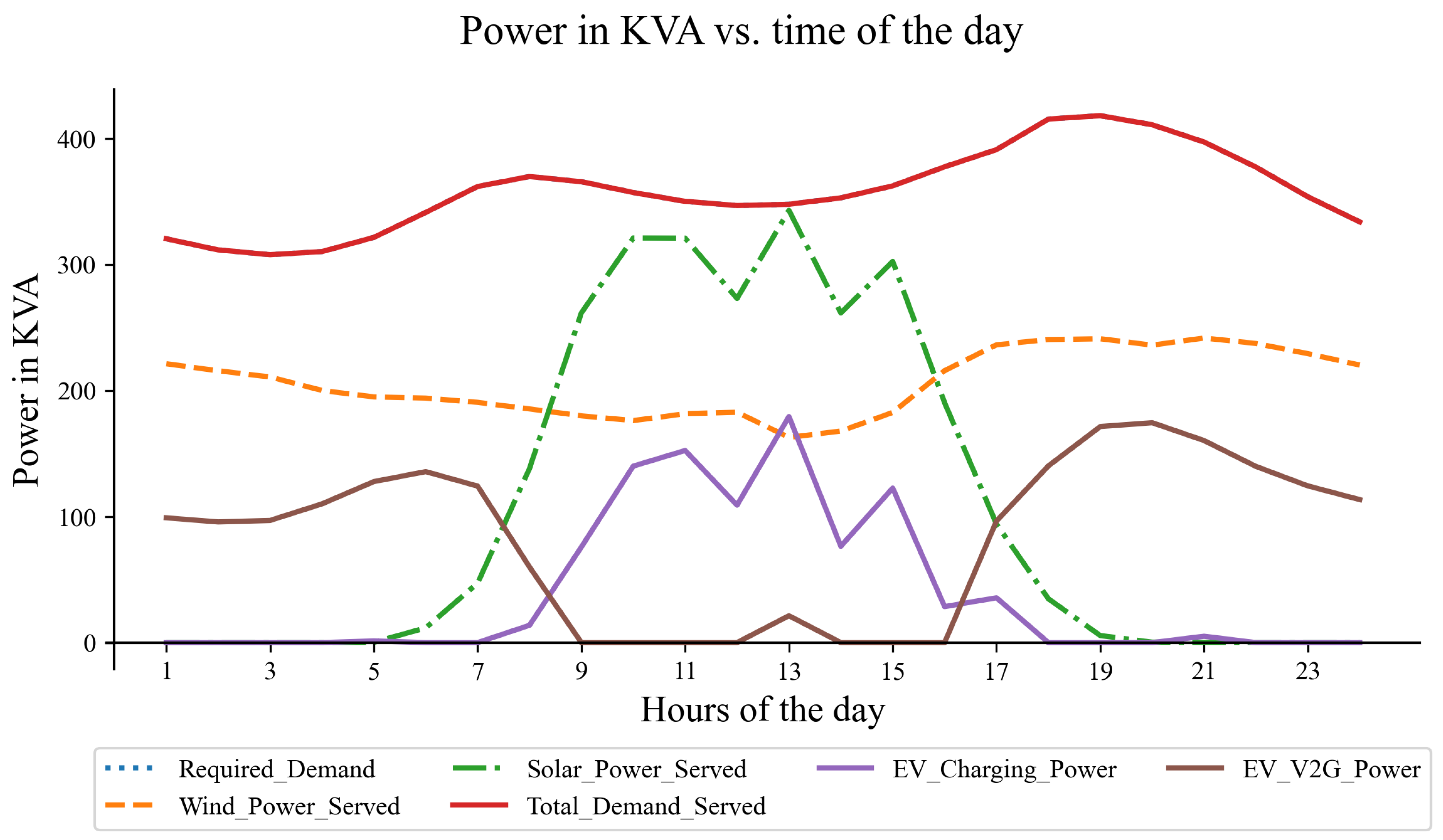
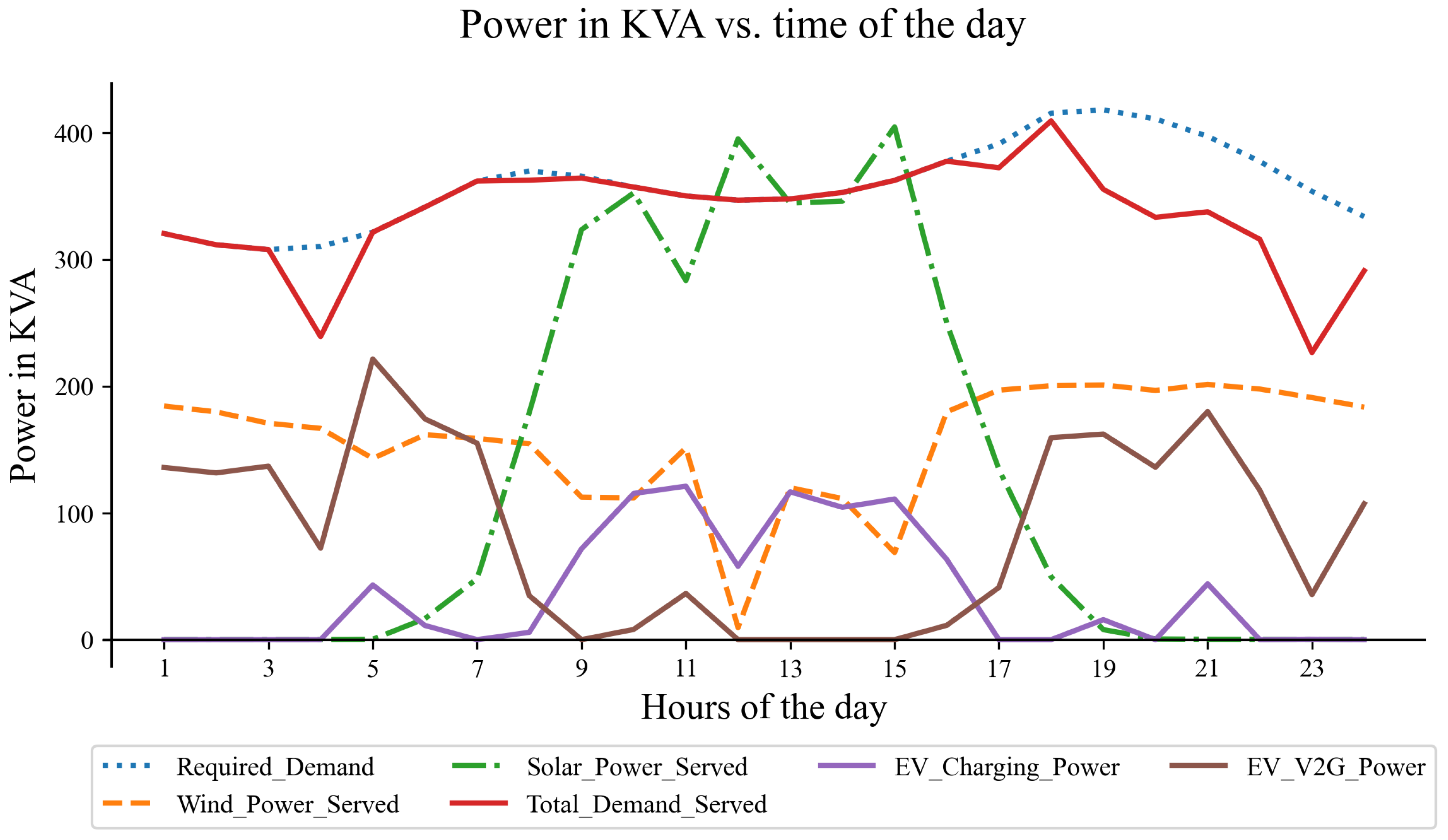
The final section of the paper showcases case studies and sensitivity analysis plots, illustrating how output power fluctuates due to uncertainty in renewable energy sources and the absence of EVs. The findings from this paper carry significant implications for the future development of sustainable, resilient, and efficient microgrids. The case study plot for normal operating conditions shows how EVs can contribute to serving total demand in a microgrid using V2G. So, EVs can be part of an environmentally friendly and economically viable energy future, reducing the burden on renewable energy sources.

2. Network Topology for AC/DC Microgrid

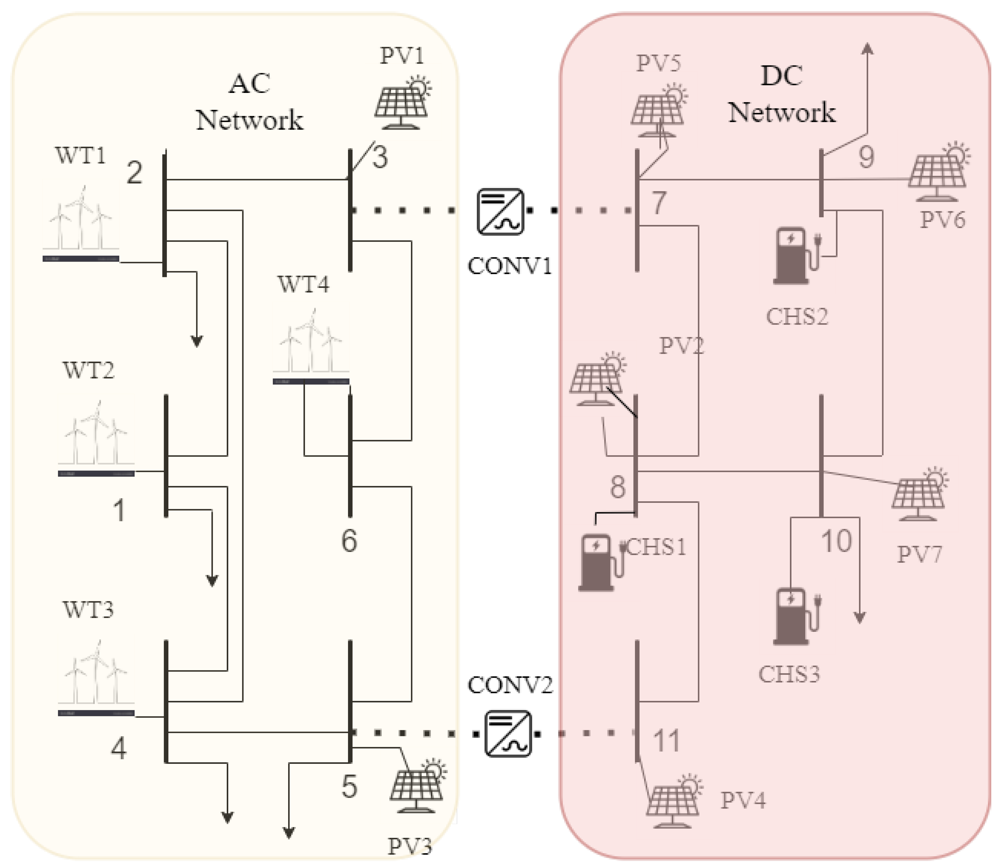
The proposed zero-carbon-emission hybrid AC/DC microgrid network is illustrated in Figure 1. This microgrid design includes 12 transmission lines divided into AC and DC components. The AC side is equipped with four wind turbine units stationed at bus numbers 1, 2, 4, and 6, given that wind turbines generate AC electricity, making them compatible with the existing AC power grid infrastructure.

Conversely, the DC side comprises seven photovoltaic (PV) solar generation units and three EV charging stations. These solar units, producing DC electricity, are strategically placed at bus numbers 3, 5, 7, 9, 10, 8, and 11 to facilitate direct power distribution. The EV charging stations are connected to bus numbers 8, 9, 10, and on the DC side, they simplify the charging infrastructure and minimize energy losses associated with power conversion [25].

As stated in the Introduction, a hybrid microgrid is considered in this work. In [16], different components of hybrid microgrids were explained, followed by developing the hybrid microgrid planning model to determine the optimal DER generation mix, the point of connection of DERs to feeders, and the type of each feeder, i.e., either AC or DC. Based on this work, this system also includes two bi-directional AC/DC converters between buses 3–7 and 5–11. These converters play a crucial role in managing the power load of the microgrid system, ensuring a smooth integration between the AC and DC components, and enhancing the system’s overall reliability.

The motivation behind incorporating solar and wind sources in this model is that they are widely used renewable energy sources. Furthermore, the inclusion of charging stations is driven by their emerging role as upcoming energy distribution centers. Charging stations offer a strategic solution to alleviate the burden on renewable energy sources during periods of low output. The sizing or capacities of these units are assumed to have a specific value; these are just candidates given physical feasibility and can be scaled and extended according to the model. The utilization of solar and wind energy resources varies depending on the time of day. Solar units contribute primarily during the day, while wind turbines are most productive in the early morning and late evening hours.

2.1. High-Level System Architecture

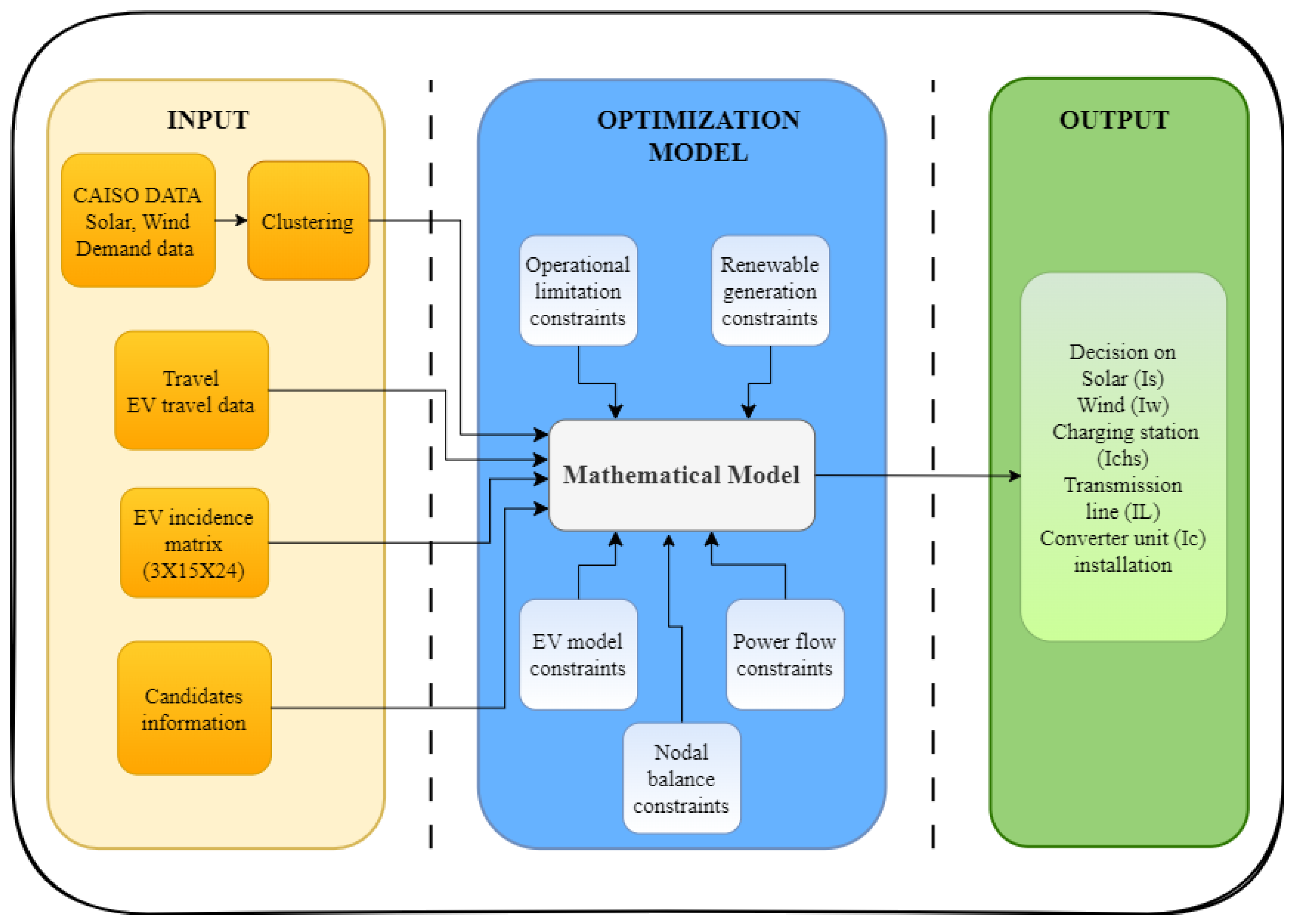
Figure 2 depicts the high-level software components incorporated in this study. The system architecture is divided into three parts: the input to the model, the optimization model, and the model’s output.

The input component consists of several sub-components:

• CAISO Data: Real-time solar, wind, and demand data collected from the CAISO website [26]. These data are then segmented into seven parts using the k-means clustering machine learning algorithm.
• EV Travel Data: These data outline the hourly travel patterns of EVs when not connected to charging stations.
• EV Incidence Matrix: This matrix documents which charging station each EV is connected to at each hour of the day.
• Candidate Information: These input data include candidate information for solar units, wind units, transmission lines, charging stations, and converters.

The second component, the optimization model, is constructed using the Julia high-level scientific programming language and optimized using the Gurobi optimization library. Different constraints on the model are:

• Renewable generation constraints;
• Nodal balance constraints;
• Power flow constraints;
• Operational limitation constraints;
• EV model constraints.

The output from the optimization model presents a 10-year plan to minimize costs for all microgrid candidates. This output is represented as binary variables and specifies when and whether each solar unit, wind unit, transmission line, converter, and charging station should be installed. The model also considers penalties for not serving the load.

The third section presents the problem formulation, including the objective function, constraints, and design considerations. In the fourth section, the focus is placed on the collection and processing of actual data to ensure the problem statement is informed by real-world data. A machine learning algorithm is employed to handle the large-scale data processing. The final section of the manuscript showcases case studies and sensitivity analysis plots.

3. Optimization Framework of the Microgrid

The optimization is performed on a model which outlines the quantity of distributed energy resources (DERs) participating in the optimization, alongside the constraints, the correlation of the control variables to the objective function, and more. Network configuration for the planning of AC/DC microgrids is studied in [27]. Mixed-integer nonlinear programming (MINLP) that minimizes the levelized planning cost, subject to system and component constraints, is considered in [27]. This section of the paper elucidates how the objective function is defined and all the constraints considered for optimization, with the end goal of minimizing the objective function. Key aspects of the problem formulation discussed in this Section include:

• Description and definition of the objective function;
• Operational limitation constraints;
• Renewable generation constraints;
• Power flow constraints;
• Nodal balance constraints;
• EV model constraints.

3.1. Objective Function

We are addressing a planning problem employing a mixed-integer optimization technique. The primary objective here is to minimize the cost of the microgrid through strategic resource planning. To achieve this, binary decision variables are used to create a schedule for resource utilization, determining when and where specific solar or wind power plants should be installed.

The objective function of the zero-carbon-emission AC/DC hybrid microgrid, aimed at minimizing costs, is chiefly formulated using these binary decision variables for the installation planning of a microgrid. These binary decision variables help determine optimized planning for installing particular resources such as solar power plants, wind power plants, converters, or transmission lines over the plan’s duration (a ten-year period is considered in this work, though it can be extended to any desired duration). The binary decision variables reveal the optimal installation time for a particular resource. Each year, the cost of installation is presumed to increase due to economic inflation or overall market trends. For simplicity, a monotonically increasing rate of installation cost is considered.

The objective function comprises several terms. The first term represents the cost of installing a solar unit, which is the product of the solar binary variable and the increasing rate of solar installation cost per year. Similarly, the second term represents the cost of wind unit installation, the third term is for the converter unit, and the fourth term is for charging station units. The final term in the objective function accounts for the penalty incurred for not meeting load requirements (lost load). Our aim is to minimize these costs to derive an optimal solution. The operational cost of renewable generation units (solar and wind) is assumed to be negligible.

In this objective function, the unit costs, penalty cost, and demand values serve as parameters, with their values already provided to the model. The model then generates output binary variables indicating the existence of a particular unit post-optimization. Such problems can be solved using various solvers from different programming languages. For this work, we have used the Gurobi optimization solver from the Julia programming language.

$$\begin{array}{c}min{\displaystyle \sum _s}{\displaystyle \sum _y}(C_s/({(1+r)}^{y-1})·(I_s^y-I_s^{y-1})+{\displaystyle \sum _w}{\displaystyle \sum _y}(C_w/({(1+r)}^{y-1})·(I_w^y-I_w^{y-1})\hfill \\ +{\displaystyle \sum _c}{\displaystyle \sum _y}(C_c/({(1+r)}^{y-1})·(I_c^y-I_c^{y-1})+{\displaystyle \sum _l}{\displaystyle \sum _y}(C_l/({(1+r)}^{y-1})·(I_l^y-I_l^{y-1})\hfill \\ +{\displaystyle \sum _{chs}}{\displaystyle \sum _y}(C_{chs}/({(1+r)}^{y-1})·(I_{chs}^y-I_{chs}^{y-1})\hfill \\ +K\ast {\displaystyle \sum _i}{\displaystyle \sum _y}{\displaystyle \sum _d}{\displaystyle \sum _t}((\overline{P_d}\ast P_d^N)-Ped)\hfill \end{array}$$

(1a)

3.2. Constraints of the Model

3.2.1. Operational Limitation Constraints

Several constraints, such as operational limitations, power flow, nodal balance, and EV-related constraints (charging, discharging, vehicle-to-grid (V2G), and travel patterns), are considered for optimization. Constraints define maximum and minimum limitations on certain variables to yield the optimal system output. As denoted in (2a), the voltage magnitude of all the buses at any time, day type, and year should fall within a given limit. Similarly, converter real power (2b) and converter reactive power (2c) should remain within their respective limits to avoid voltage drops due to increased reactive power. Power limits for each transmission line on the AC and DC sides are also enforced as per (2d) and (2f). These operational limitation constraints apply to each bus/line, time of the day, day type, and year.

$$\begin{array}{cc}& \underline{V}\le V_{i,t}^{d,y}\le \overline{V}\hfill \end{array}$$

(2a)

$$\begin{array}{cc}& \underline{P_c}\le P_{c,t}^{d,y}\le \overline{P_c}\hfill \end{array}$$

(2b)

$$\begin{array}{cc}& \underline{Q_c}\le Q_{c,t}^{d,y}\le \overline{Q_c}\hfill \end{array}$$

(2c)

$$\begin{array}{cc}& {\underline{S}}_{l,t}^{d,y}\le S_{ac,l,t}^{d,y}\le {\overline{S}}_{l,t}^{d,y}\hfill \end{array}$$

(2d)

$$\begin{array}{cc}& S_{ac,l,t}^{d,y}=P_{ac,l,t}^{d,y}+\xi ·Q_{ac,l,t}^{d,y}\hfill \end{array}$$

(2e)

$$\begin{array}{cc}& {\underline{S}}_{l,t}^{d,y}\le P_{dc,l,t}^{d,y}\le {\overline{S}}_{l,t}^{d,y}\hfill \end{array}$$

(2f)

3.2.2. Renewable Generation Constraints

The network topology for the hybrid (AC/DC) microgrid includes seven solar generation units and four wind generation units. The power output from these renewable units is contingent on various conditions. As indicated by constraints (3a) and (3b), wind and solar power output must be greater than zero and less than the maximum forecast output of each unit. This allows for necessary curtailments due to operational limitations [11]. The predicted output of solar or wind is the product of solar irradiance and wind flow with the capacity of the respective unit.

Although solar and wind units do not generate reactive power since their output is DC, the inverters used to convert power from DC to AC generate reactive power. Therefore, it is considered that inverters used for solar and wind generation produce reactive power in both positive and negative values, which are limited by the active power generated by those units as depicted in (3c) and (3b). Excessive reactive power generation by the inverters can induce voltage fluctuations and other grid problems, leading to power outages and further issues. Therefore, limiting reactive power in a solar PV system is crucial as it impacts the stability and efficiency of the microgrid [28].

All the values of renewable generation constraints apply to each generation unit, each time of the day, day type, and year.

$$\begin{array}{cc}& 0\le P_{w,t}^{d,y}\le P_{F,w,t}^{d,y}\hfill \end{array}$$

(3a)

$$\begin{array}{cc}& 0\le P_{s,t}^{d,y}\le P_{F,s,t}^{d,y}\hfill \end{array}$$

(3b)

$$\begin{array}{cc}& -P_{w,t}^{d,y}\le Q_{w,t}^{d,y}\le P_{w,t}^{d,y}\hfill \end{array}$$

(3c)

$$\begin{array}{cc}& -P_{s,t}^{d,y}\le Q_{s,t}^{d,y}\le P_{s,t}^{d,y}\hfill \end{array}$$

(3d)

By controlling the amount of reactive power generated within the system, grid operators can maintain its safe and reliable operation without creating issues for other users of the microgrid. Nevertheless, the imposed constraints on renewable generation units impede the microgrid integration, thereby challenging the enhancement in the overall stability and efficiency of the electrical grid.

3.2.3. Power Flow Constraints

Power flow constraints on the AC side of the system dictate the balance between real and reactive power. These constraints are subject to parameters such as conductance, admittance, voltage, and voltage angle between any two buses. Conductance is a measure used to model the power losses in transmission lines due to resistive heat dissipation. As such, a transmission line with higher conductance is less efficient because it loses more power as heat. Equations (4b)–(4d) represent the AC power flow for real and reactive power. In Equation (4b), the first term describes the power dissipation through heat on the transmission line between bus j and bus o, which is dependent on the voltage difference between these two buses. The second term represents the product of the voltage angle difference between the two buses and the line susceptance.

$$\begin{array}{cc}& P_{ac,l,t}^{d,y}\le -G_{jo}\ast (V_{j,t}^{d,y}-V_{o,t}^{d,y})+B_{jo}\ast ({\theta }_{j,t}^{d,y}-{\theta }_{o,t}^{d,y})+M\ast (1-I_l^y)\hfill \end{array}$$

(4a)

$$\begin{array}{cc}& P_{ac,l,t}^{d,y}\ge -G_{jo}\ast (V_{j,t}^{d,y}-V_{o,t}^{d,y})+B_{jo}\ast ({\theta }_{j,t}^{d,y}-{\theta }_{o,t}^{d,y})-M\ast (1-I_l^y)\hfill \end{array}$$

(4b)

$$\begin{array}{cc}& Q_{ac,l,t}^{d,y}\le B_{jo}\ast (V_{j,t}^{d,y}-V_{o,t}^{d,y})+G_{jo}\ast ({\theta }_{j,t}^{d,y}-{\theta }_{o,t}^{d,y})+M\ast (1-I_l^y)\hfill \end{array}$$

(4c)

$$\begin{array}{cc}& Q_{ac,l,t}^{d,y}\ge B_{jo}\ast (V_{j,t}^{d,y}-V_{o,t}^{d,y})+G_{jo}\ast ({\theta }_{j,t}^{d,y}-{\theta }_{o,t}^{d,y})-M\ast (1-I_l^y)\hfill \end{array}$$

(4d)

$$\begin{array}{cc}& P_{dc,l,t}^{d,y}\le \frac{V_{j,t}^{d,y}-V_{o,t}^{d,y}}{r_l}+M\ast (1-I_l^y)\hfill \end{array}$$

(4e)

$$\begin{array}{cc}& P_{dc,l,t}^{d,y}\ge \frac{V_{j,t}^{d,y}-V_{o,t}^{d,y}}{r_l}-M\ast (1-I_l^y)\hfill \end{array}$$

(4f)

3.2.4. Nodal Balance Constraints

Nodal balance constraints ensure that the power flow into and out of any bus or line remains consistent at each hour of the day, each type of day, and throughout the year. These constraints abide by the fundamental principle that the rate of energy change at any given time equals the power at the network port minus the dissipated power. Equation (5a) enforces the condition that the total load served by the microgrid at any bus, time, day, and year should be equal to the summation of the net transmitted power from different sources (e.g., solar, wind, converter, transmission line) and the difference between the vehicle-to-grid (V2G) power and EV charging power. Equation (5b) applies to converters and transmission lines, as the reactive power of solar and wind is not considered. It pertains to the AC side of the system. Equation (5c) provides the nodal balance equation for the DC side of the microgrid.

$$\begin{array}{cc}& \begin{array}{c}\hfill \sum _{e\in {\mathcal{E}}_i}(P_{v2g,e,t}^{d,y}-P_{ch,e,t}^{d,y})+\sum _{w\in {\mathcal{W}}_i}{P}_{w,t}^{d,y}+\sum _{s\in {\mathcal{S}}_i}{P}_{s,t}^{d,y}\\ \hfill +\sum _{c\in {\mathcal{C}}_i}{P}_{c,t}^{d,y}+\sum _{l\in {\mathcal{L}}_i^{to}}{P}_{ac,l,t}^{d,y}-\sum _{l\in {\mathcal{L}}_i^{fr}}{P}_{ac,l,t}^{d,y}=P_{ed,i,t}^{d,y}\end{array}\hfill \end{array}$$

(5a)

$$\begin{array}{cc}& \begin{array}{c}\hfill +{\displaystyle \sum _{c\in {\mathcal{C}}_i}}{Q}_{c,t}^{d,y}+{\displaystyle \sum _{l\in {\mathcal{L}}_i^{to}}}{Q}_{ac,l,t}^{d,y}-{\displaystyle \sum _{l\in {\mathcal{L}}_i^{fr}}}{Q}_{ac,l,t}^{d,y}=Q_{ed,i,t}^{d,y}\end{array}\hfill \end{array}$$

(5b)

$$\begin{array}{cc}& \begin{array}{c}\hfill \sum _{e\in {\mathcal{E}}_i}(P_{v2g,e,t}^{d,y}-P_{ch,e,t}^{d,y})+\sum _{w\in {\mathcal{W}}_i}{P}_{w,t}^{d,y}+\sum _{s\in {\mathcal{S}}_i}{P}_{s,t}^{d,y}\\ \hfill +\sum _{c\in {\mathcal{C}}_i}{P}_{c,t}^{d,y}+\sum _{l\in {\mathcal{L}}_i^{to}}{P}_{dc,l,t}^{d,y}-\sum _{l\in {\mathcal{L}}_i^{fr}}{P}_{dc,l,t}^{d,y}=P_{ed,i,t}^{d,y}\end{array}\hfill \end{array}$$

(5c)

All these equations are grounded in Kirchhoff’s law, which stipulates that the total current flowing into a bus or line in any electric grid equals the current flowing out. These constraints must be satisfied to maintain network stability and reliability, preventing power outages and voltage instability.

3.2.5. Ev Model Constraints

Electric vehicles (EVs) are incorporated into the design to leverage benefits such as their storage capacity, V2G power for meeting peak demand, and demand response capabilities. However, to effectively harness these advantages, proper management and planning are essential for the integration of EVs within the constraints of the microgrid. EVs can operate in one of three modes. In the traveling mode, power is converted from DC to AC by an inverter and then directed to the electric motor, thereby consuming energy. In the plugged-in mode, EVs can either charge using an external power source, such as a charging station or standard electrical outlet or send power back to the grid (V2G) if the charger is bidirectional. V2G is a smart charging strategy that enables EVs to charge during off-peak hours and supply power to the grid during peak hours, when there is an additional energy demand. The third mode, idle or parking mode, does not involve any energy exchange, keeping the EV’s energy state constant.

Equation (6a) restricts the charging power of EVs to be greater than or equal to zero and less than the maximum value defined in the model. Equation (6b) governs the discharging power of EVs, ensuring it lies within the range of zero and the maximum discharging power. As an EV can either be in charging or V2G mode, Equation (6c) models this constraint. The energy stored in the EV is bounded by its maximum and minimum values as per Equation (6e). Finally, Equation (6f) asserts that the energy stored in the EVs at any given time equals the summation of the energy stored an hour prior, the charging power at that time, and the difference between the discharging power and V2G power. These constraints should be met to integrate EVs successfully with renewable energy sources within the proposed microgrid.

$$\begin{array}{cc}& 0\le P_{ch,e,t}^{d,y}\le I_{ch,e,t}^{d,y}\ast {\overline{P}}_{ch,e}\hfill \end{array}$$

(6a)

$$\begin{array}{cc}& 0\le P_{v2g,e,t}^{d,y}\le I_{v2g,e,t}^{d,y}\ast {\overline{P}}_{v2g,e}\hfill \end{array}$$

(6b)

$$\begin{array}{cc}& I_{ch,e,t}^{d,y}+I_{v2g,e,t}^{d,y}\le {\left(IncidanceMatrix\right)}_{ch,e,t}^d\ast I_{ch}^y\hfill \end{array}$$

(6c)

$$\begin{array}{cc}& 0\le P_{dch,e,t}^{d,y}\le \frac{I_{dch,e,t}\ast P_{tr,t}^d\ast 0.3}{1000}\hfill \end{array}$$

(6d)

$$\begin{array}{cc}& {\underline{P}}_{ev,e}\le P_{ev,e,t}^{d,y}\le {\overline{P}}_{ev,e}\hfill \end{array}$$

(6e)

$$\begin{array}{cc}& P_{ev,e,t}^{d,y}=P_{ev,e,t-1}^{d,y}+P_{ch,e,t}^{d,y}-P_{dch,e,t}^{d,y}-P_{v2g,e,t}^{d,y}\hfill \end{array}$$

(6f)

4. Data Collection and Data Processing

As this work contemplates, planning a zero-carbon-emission microgrid demands careful and proactive management of renewable generation units. This is in view of the uncertainties and challenges these sources pose to the optimal operation of the microgrid. Renewable sources, such as solar and wind, do not operate in a deterministic pattern. Various factors such as weather patterns, seasonal variations, and natural disasters can affect the availability of these energy resources. Such dynamics render the reliable operation and integration of renewable sources into a microgrid a complex task.

Although we have designed a microgrid for an assumed area of interest based on a given topology and have modeled an optimization problem for resource utilization planning to minimize the cost, we cannot feed any hypothetical data into this model. Instead, it must be logical, feasible, and realistic. Consequently, we have used the actual California data, available on the CAISO website [26], and processed it to fit our model.

Data gathering for this purpose consists of three major aspects:

• Data collection;
• Data normalization;
• Data clustering.

This section presents an overview of the data processing tasks. Section 4.1 describes how we derived the solar, wind, and demand energy data from CAISO. Section 4.2 elucidates how we applied machine learning algorithms for demand data. Section 5 provides visual representations of the normalized solar, wind, and demand values in the form of tables and plots. Section 5.1 offers a comprehensive overview of the incidence matrix of Electric Vehicles (EVs). Section 5.2 showcases the travel pattern of EVs over 24 h via heatmap plotting.

4.1. Solar, Wind, and Demand Data Generation

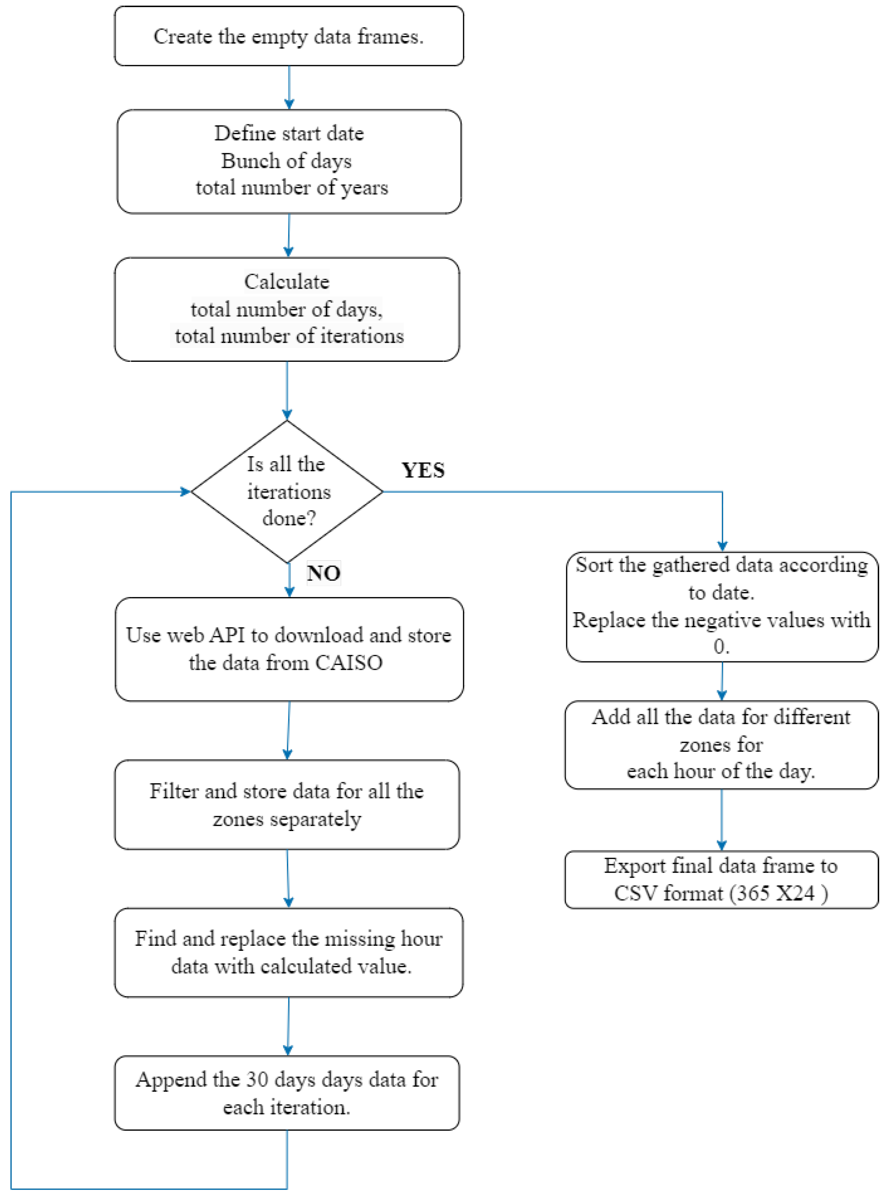
The CAISO, a non-profit organization that oversees the high-voltage power grid across much of California, provides diverse data pertinent to the grid’s operation and management. These data encompass the total solar and wind generation for every hour of every day throughout the year, spanning the entire region of California.

We assume these data to accurately represent the relative amount of solar and wind energy available across the region. The method adopted for this work, as outlined in Figure 3, is explained below:

• We first install all necessary packages in the Julia software, namely, CSV, data frames, LightXML, http, and zip file.
• Empty data frames are created to house the data obtained from CAISO. For instance, solar power output data are segmented into three distinct zones of the California region, NP15, SP15, and ZP26, with the zones defined by area. Wind power output data are available for the NP15 and SP15 regions. Energy demand values encompass the entire California region.
• To access the data, the following parameters are established:
  • Start Date = 12/31/201900:00;
  • Hours Of Days = 24;
  • Bunch Of Days = 30;
  • Days Of Year = 365;
  • Number Of Years = 1 or 2;
  • Total Number Of Days = Number Of Years × Days Of Year;
• We calculate the number of iterations as $(\mathrm{Total}\mathrm{Number}\mathrm{Of}\mathrm{Days}/\mathrm{Bunch}\mathrm{Of}\mathrm{Days})+1$ since CAISO does not permit data download for more than 30 days at a time.
• We use the Web API in Julia to download the required data from CAISO in 30-day increments.
• These data are then filtered according to zones and stored in the separate data frames we created. All values are expressed in the Megawatt (MW) unit.
• It was observed that data were missing for specific days, so we filled gaps with the mean of the previous and next hour values.
• For every iteration, data are appended to the respective data frames until all iterations are complete.
• Once all data are stored, they are sorted according to the date. All negative values are replaced with 0.
• To generate the final data frame, similar hours of data, i.e., 1 to 24, are aggregated across all different zones. The final data frame is exported in CSV format. These data cover 365 days and 24 h, resulting in data frames of size 365 × 24 for solar output, wind output, and demand data.

4.2. Clustering

The subsequent stage of data processing is clustering. The intent here is to diminish the data volume to streamline calculations, without compromising the integrity of the original data. Clustering constitutes a process wherein similar data elements are grouped into predefined sets. This study focuses on clustering demand data to significantly reduce the volume of data that the optimization algorithm must process.

Clustering is a prominent unsupervised machine learning technique for pattern recognition and data analysis. In this work, we employ k-means clustering to discern patterns in the CAISO data, logically condense the dataset, and group similar items together. K-means clustering, a partitioning method, facilitates the classification of objects into ‘k’ distinct groups or clusters. This technique requires pre-specifying the number of ‘k’ clusters [29].

The demand for electricity in any region can be influenced by several factors, including:

• Natural Disasters: Tornadoes, ice storms, heatwaves, floods, and wildfires can significantly affect electricity demand.
• Seasonal Variations: Shifts in temperature and weather patterns influence electricity consumption. For example, electricity demand may spike during the summer months due to an increased use of air conditioning.
• Technological Advancements: Rapid industrialization, novel electrical appliances, and technological advancements can also alter electricity demand patterns.
• Energy Prices and Government Policies: Fluctuations in electricity prices and changes in government policies can affect electricity consumption habits, leading to variable demand patterns.

Given these factors, it is reasonable to assume that demand can be segmented into seven unique categories representative of different days throughout the year. The cluster size considered in this work is the assumption for different types of days based on changes in demand. This size can be varied if the demand changes for specific days in a year is known. We apply clustering to group these seven categories based on the similarity of demand values, significantly simplifying computations compared to dealing with large data spanning 365 days, each with 24 h.

As previously stated, California’s CAISO data offers solar, wind, and energy demand information for each hour, day, and year. Handling this massive volume of data requires a systematic approach. Therefore, we employ clustering to regroup the data into seven clusters and compute new average values within these clusters. The steps outlined in Figure 4 demonstrate this process:

• Demand data from CAISO, collected using a web API over two years and stored in two data frames, are imported into Julia. Each data frame contains demand values for 365 days and 24 h (365 × 24) of the corresponding year.
• The data cleansing stage involves converting the data from Universal Time Coordinated (UTC) to Pacific Time (PT), since CAISO data are provided in UTC while this study focuses on the California region.
• Next, we concatenate the arrays of two data frames, joining two years of data to form a 365 × 48 combined array. Following this, we transpose the matrix into a 48 × 365 format, where each row represents an hour’s demand data for all 365 days.
• We use the k-means algorithm, a popular clustering technique, to partition the dataset into ‘k’ clusters. This algorithm primarily operates by iteratively assigning each data point to the cluster with the closest mean, and subsequently recalculating the mean of each cluster based on new assignments [29]. We feed the 48 × 365 matrix into the k-means function, along with parameters such as cluster size and number of iterations (7 clusters and a maximum of 1000 iterations, in this case).
• The algorithm works iteratively by assigning each data point to the cluster with the closest mean or centroid, then recalculates the centroid of each cluster based on the new assignments. The iteration continues until no new centroid value is computed or the maximum iteration limit is reached, yielding the result as cluster assignments.
• These assignments help to determine which day aligns with which type of cluster based on data similarity. The final matrix is calculated by averaging the demand data for each cluster assignment, resulting in a 7 × 24 matrix for the seven clusters identified in this work.
• These data are normalized by identifying the maximum peak energy demand and treating it as the unity value. Data normalization standardizes the data format across the system, making it usable for any hypothetical model with maximum peak generation within the microgrid’s operational limits [30].
• Finally, the last two steps are repeated for solar and wind data to reduce the size of their matrices. Here, the same assignments are used for solar/wind data, and averages for each cluster assignment are calculated. The data are subsequently normalized to make them universally applicable for any microgrid rating.

5. Case Study Data Input

Table 1. Normalized demand values for 7 types of days.

t = 1	t = 2	t = 3	…	t = 16	…	t = 22	t = 23	t = 24
0.6384	0.6133	0.5996	…	1.000	…	0.7857	0.7221	0.6744
0.5382	0.5191	0.5097	…	0.8156	…	0.6547	0.6045	0.5667
0.4599	0.4478	0.4422	…	0.5050	…	0.5351	0.5038	0.4782
0.5579	0.5368	0.5262	…	0.8274	…	0.6854	0.6293	0.5884
0.5140	0.4974	0.4889	…	0.6821	…	0.6144	0.5713	0.5384
0.5360	0.5173	0.5081	…	0.7993	…	0.6509	0.6007	0.5635
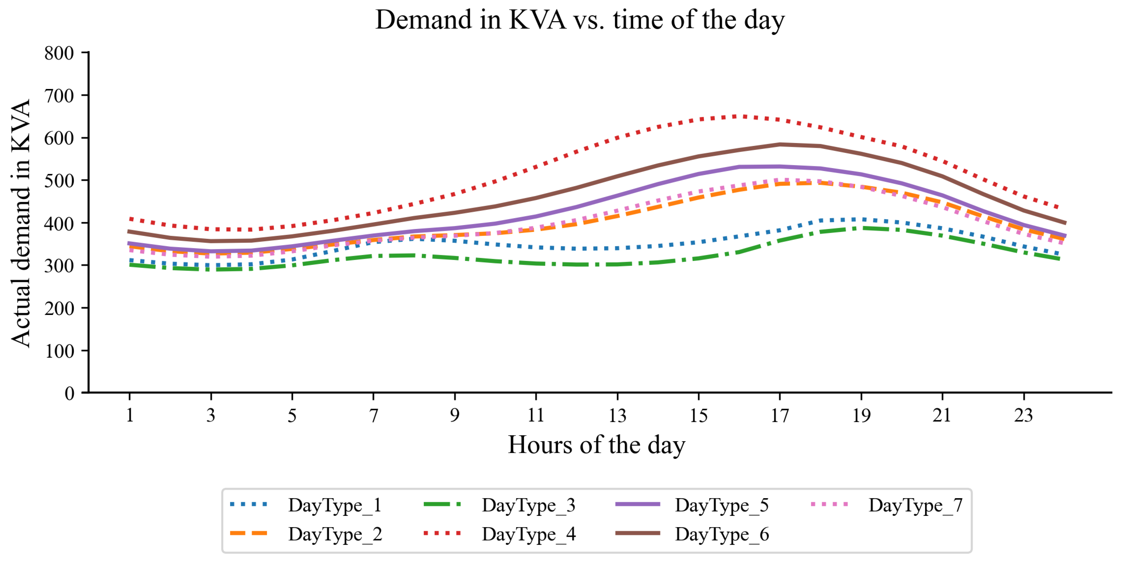
0.4787	0.4658	0.4604	…	0.5792	…	0.5648	0.5284	0.4985

presents normalized demand values for seven different types of days, where the columns denote the hour of the day, and the rows indicate the type of the day. These normalized values are employed in the calculation of actual demand. The correlation between actual demands (in KVA) and the time of day is graphically depicted in Figure 5.

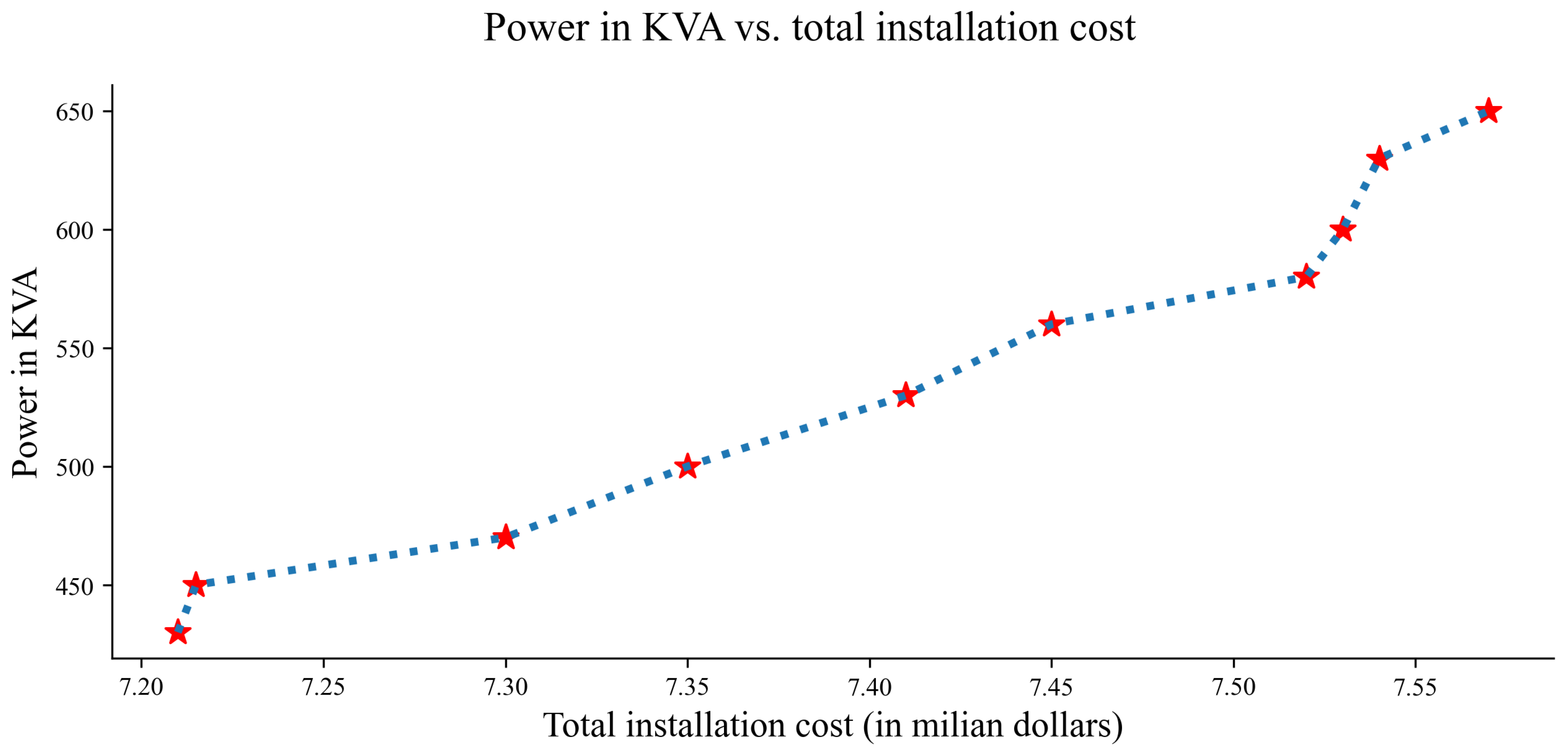
The current model’s maximum demand value is set at 650 KVA for the first year, with an anticipated increase of 2 percent per annum. The demand variations for each day type are demonstrated in Figure 5. The demand patterns for day type two and day type seven look almost similar. These data were generated by aggregating and classifying real-world demand data from the California region, obtained from the CAISO website.

Table 2. Normalized solar output values for 7 types of days.

t = 1	t = 2	t = 3	…	t = 12	…	t = 22	t = 23	t = 24
0.00032	0.00031	0.00029	…	0.9115	…	0.00030	0.00030	0.00031
0.00035	0.00035	0.00033	…	0.917	…	0.00050	0.00040	0.00035
0.00021	0.00020	0.00030	…	0.767	…	0.00028	0.00024	0.00024
0.00014	0.00012	0.00012	…	0.986	…	0.00016	0.00015	0.00014
0.00010	9.88 $\times {10}^{-5}$	9.37 $\times {10}^{-5}$	…	1.000	…	0.00018	0.00020	0.00010
7.89 $\times {10}^{-5}$	7.55 $\times {10}^{-5}$	6.09 $\times {10}^{-5}$	…	0.978	…	0.00015	0.00011	7.52 $\times {10}^{-5}$
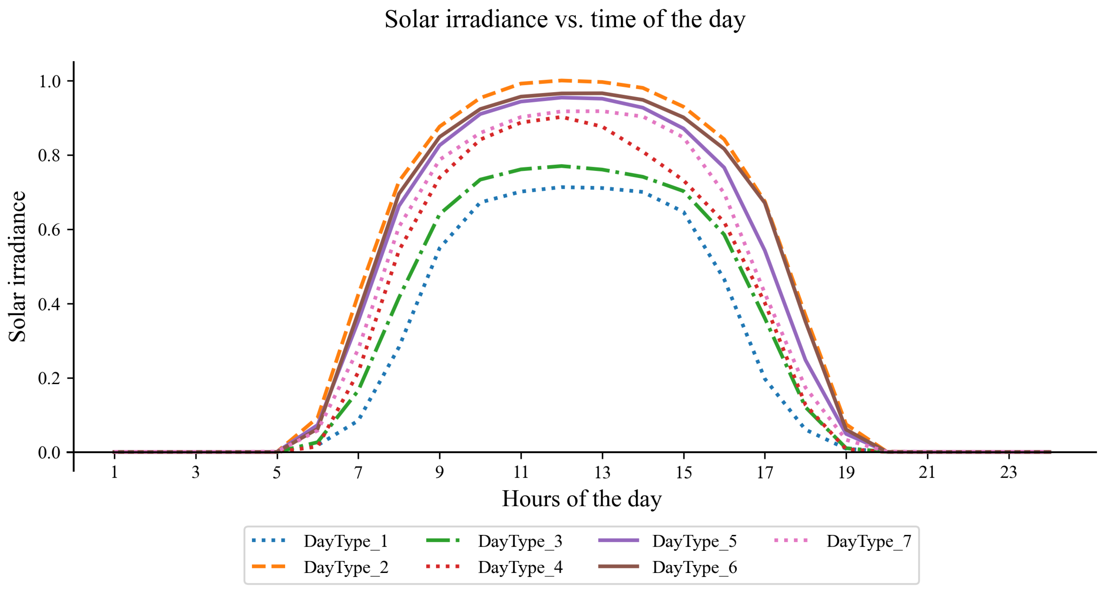
0.00039	0.00035	0.00030	…	0.736	…	0.00053	0.00044	0.00041

provides normalized solar values for seven different types of days, illustrating the variation in solar irradiance throughout the day. The maximum solar capacity of the solar unit considered in our model is 80 KVA, with seven solar units employed.

Hence, the total maximum solar output is computed as 80 × 7 = 560 KVA. Figure 6 visualizes the pattern of solar availability for each day type, highlighting the peak solar irradiance between 11 a.m. and 3 p.m.

Table 3. Normalized wind output values for 7 types of days.

t = 1	t = 2	t = 3	…	t = 12	…	t = 22	t = 23	t = 24
0.5735	0.5247	0.47	…	0.220	…	0.6670	0.6561	0.625
0.542	0.527	0.49	…	0.223	…	0.6670	0.6561	0.625
0.615	0.6092	0.590	…	0.447	…	0.6342	0.6276	0.6163
0.9841	0.9564	0.911	…	0.447	…	0.99554	1.0	0.997
0.8600	0.827	0.775	…	0.328	…	0.9434	0.9186	0.901
0.8792	0.839	0.7924	…	0.237	…	0.937	0.9170	0.899
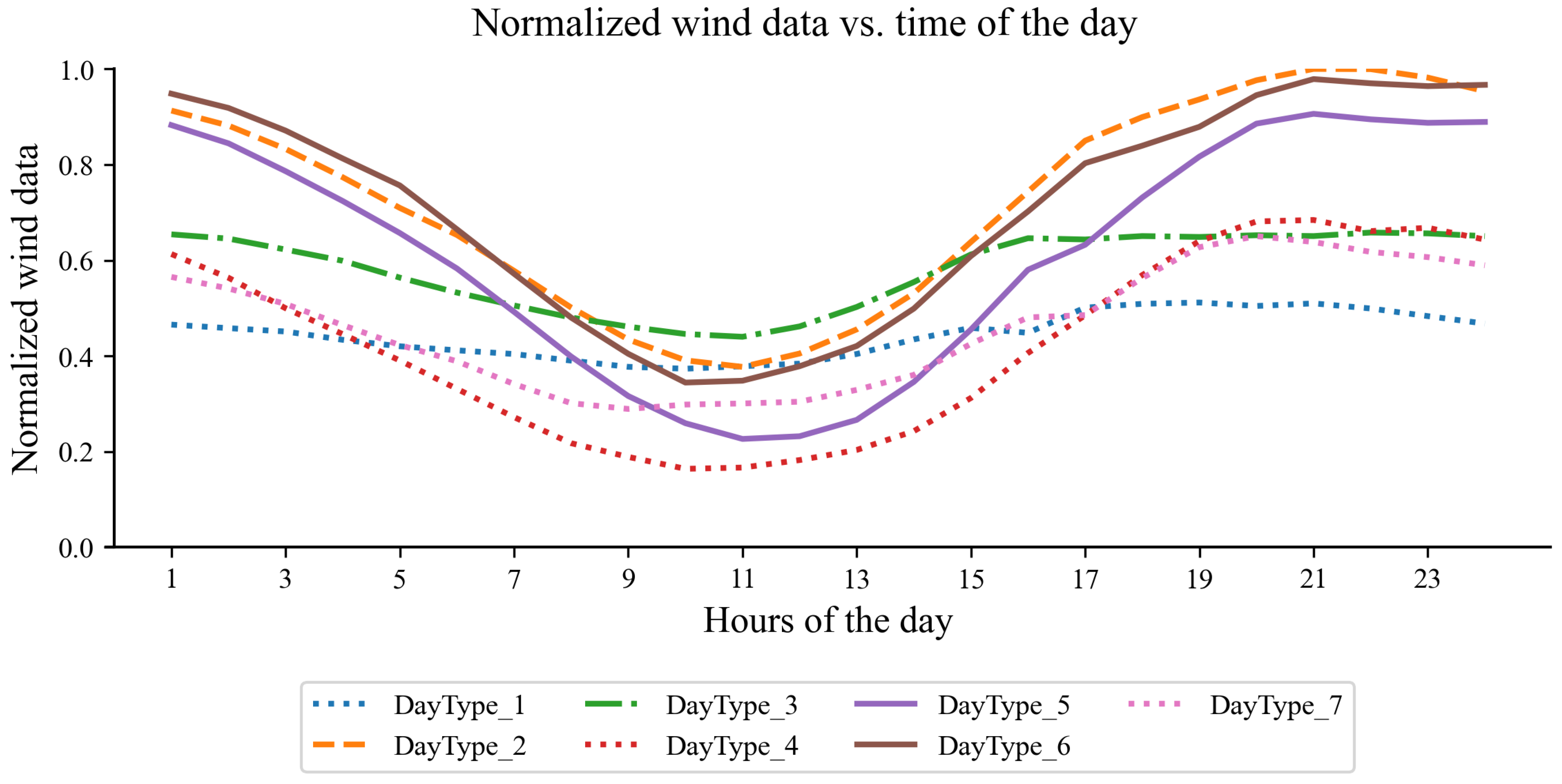
0.4504	0.4382	0.423	…	0.350	…	0.4696	0.4605	0.4515

displays normalized wind values, emphasizing the wind flow variation throughout the day. In the model, each of the four wind units has a maximum capacity of 100 KVA, leading to a total maximum wind output of 400 KVA.

The wind availability pattern is depicted in Figure 7, where the wind flow peaks between 1 a.m. and 5 a.m., and 5 p.m. and 10 p.m.

5.1. Incidence Matrix and EV Travel Pattern

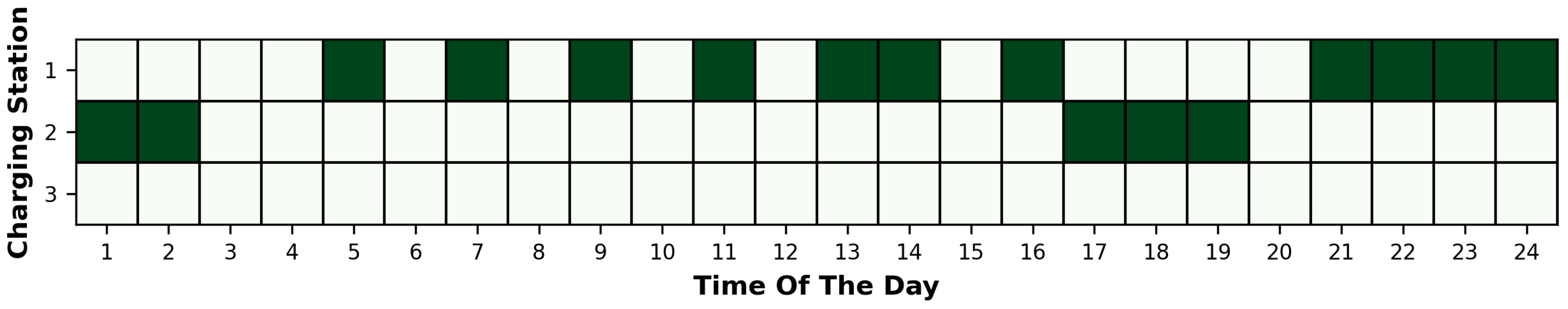
Incorporating electric vehicles in this model necessitates a realistic dataset, accompanied by appropriate constraints. Creating an incidence matrix, a simplistic binary dataset, plays a significant role in this aspect. This matrix assumes a fixed number of electric vehicles with known capacities operating in a defined area where a microgrid is implemented. Vehicles follow a known transit pattern, utilizing predefined charging locations, represented in the incidence matrix. Though real-world scenarios would exhibit greater complexity, we adhere to this pattern for the sake of this model and calculations. Incidental matrix constraints include, for example, the impossibility of an electric vehicle connecting to two charging stations simultaneously. The incidence matrix is formulated using a standard Excel template. The binary data from the incidence matrix provides essential information, indicating whether a vehicle is connected to a specific charging station at any given time. The model utilizes this information as a parameter for running the optimization algorithm.

Table 4. Miles traveled vs. time of the day.

t = 1	t = 2	t = 3	t = 4	…	t = 12	…	t = 22	t = 23	t = 24
1.3	1.7	3.2	4.2	…	10.68	…	10.8	10.5	2.7
0.95	3.06	2.98	3.84	…	10.98	…	10.8	10.5	2.7
1.5	2.8	4.2	3.10	…	6.0	…	7.5	10.45	12.46
2.1	1.6	5.03	3.99	…	2.3	…	4.8	9.17	4.06
2.4	1.2	2.41	2.92	…	4.5	…	5.9	4.2	6.6
1.3	2.15	2.06	4.4	…	4.02	…	8.41	6.40	2.36
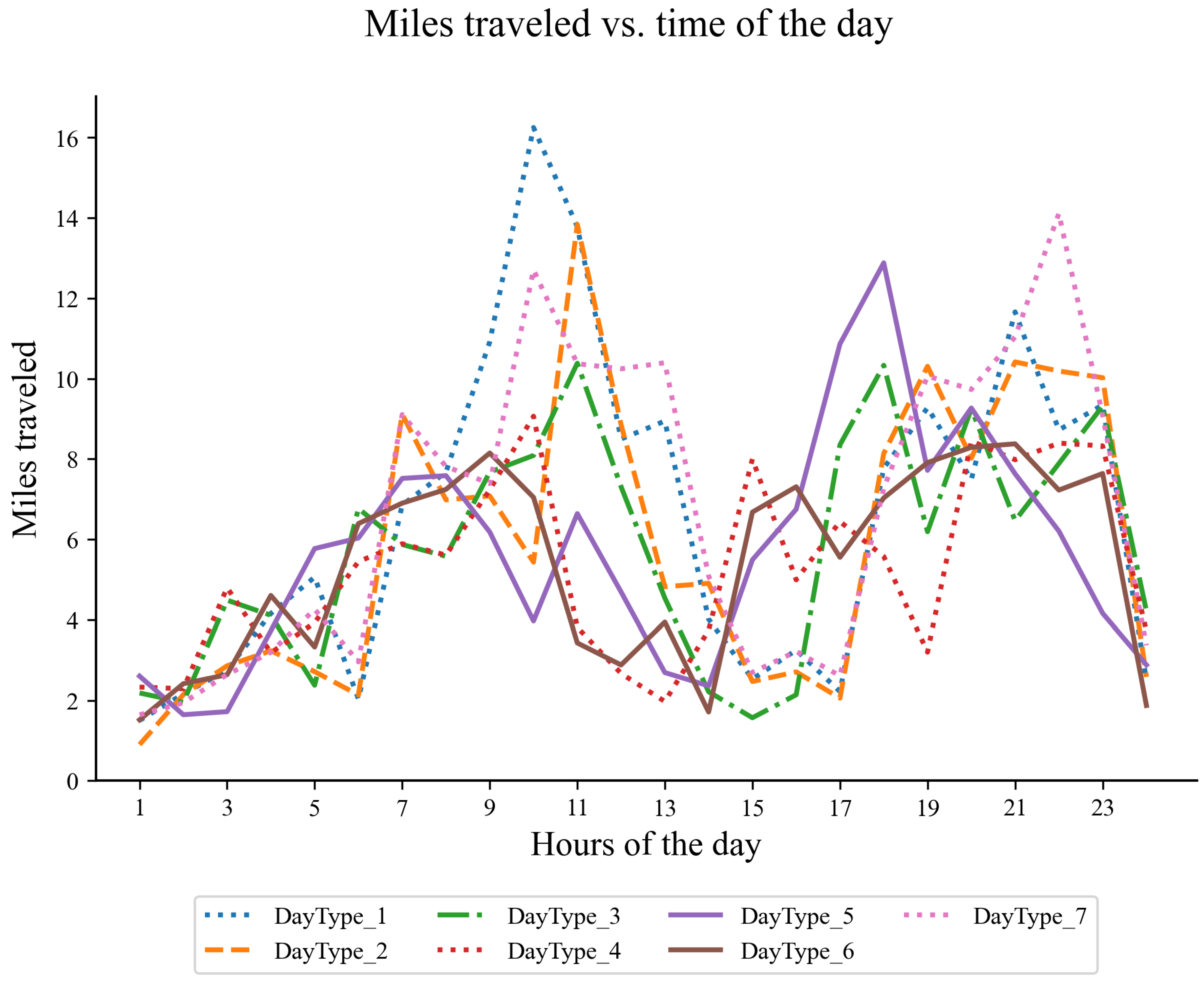
1.51	2.03	2.97	3.47	…	9.2	…	12.52	10.39	3.69

reveals the average distance (in miles) traveled by all the electric vehicles at each time of the day, while Figure 8 illustrates the vehicles’ travel pattern throughout the day. The electric vehicle discharge pattern depends upon how electric vehicles are traveling throughout the day. It means the electric vehicle is not available for charging and V2G, i.e., for giving energy back to the grid at this time.

5.2. Connection of Electric Vehicles

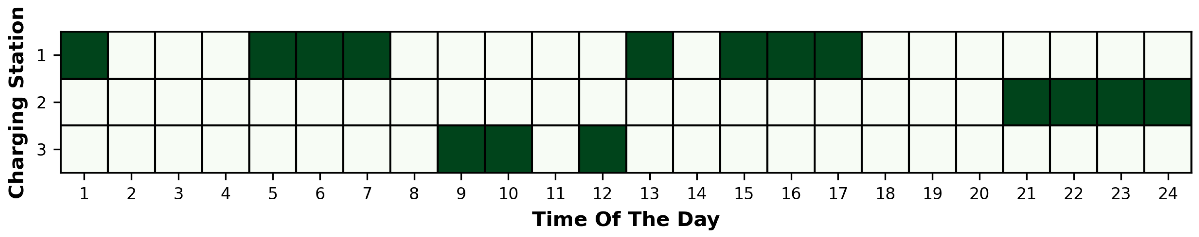
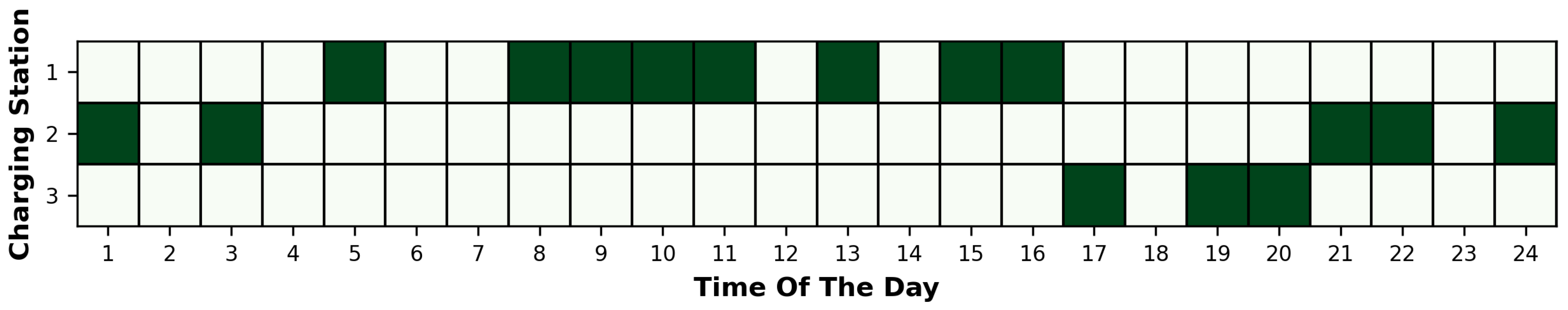
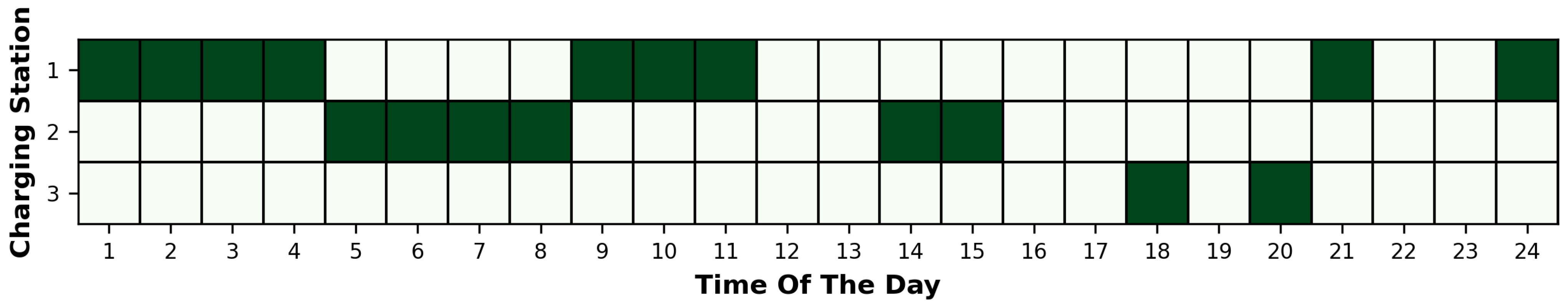
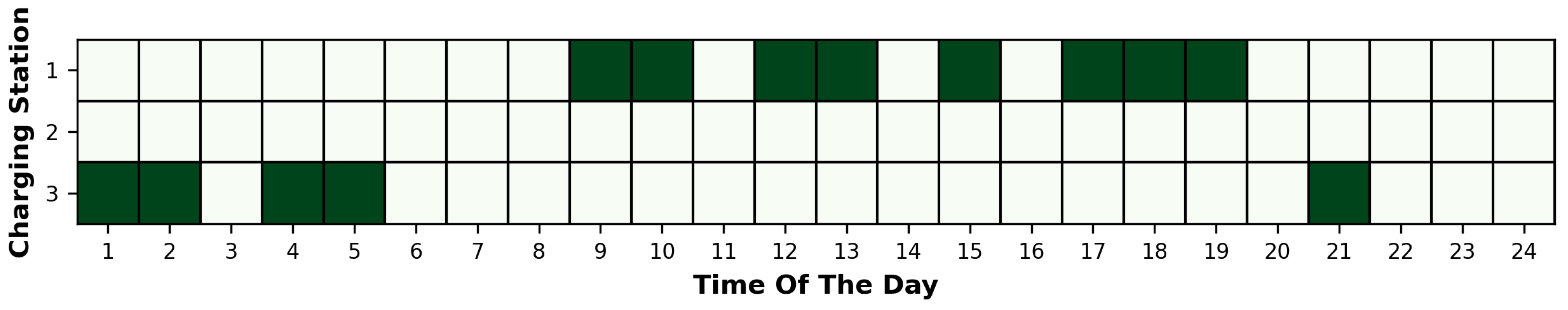
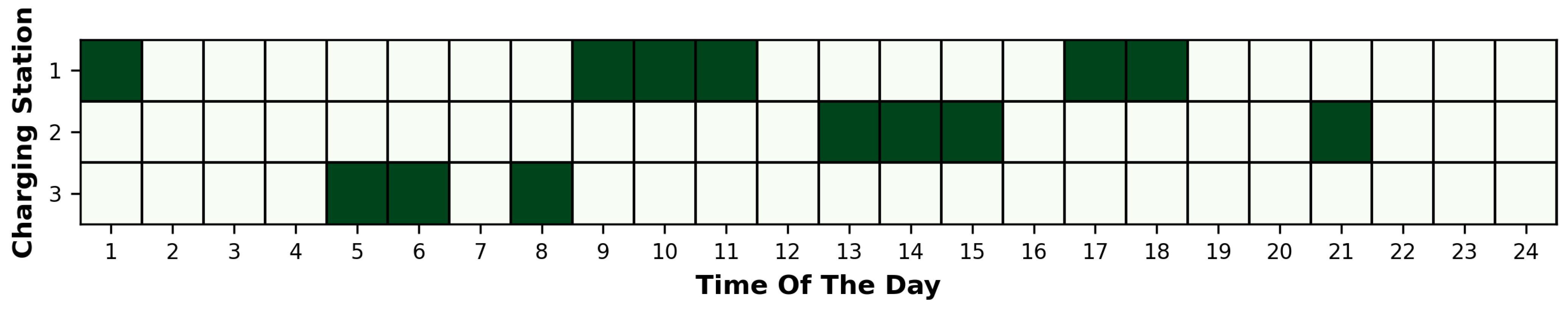
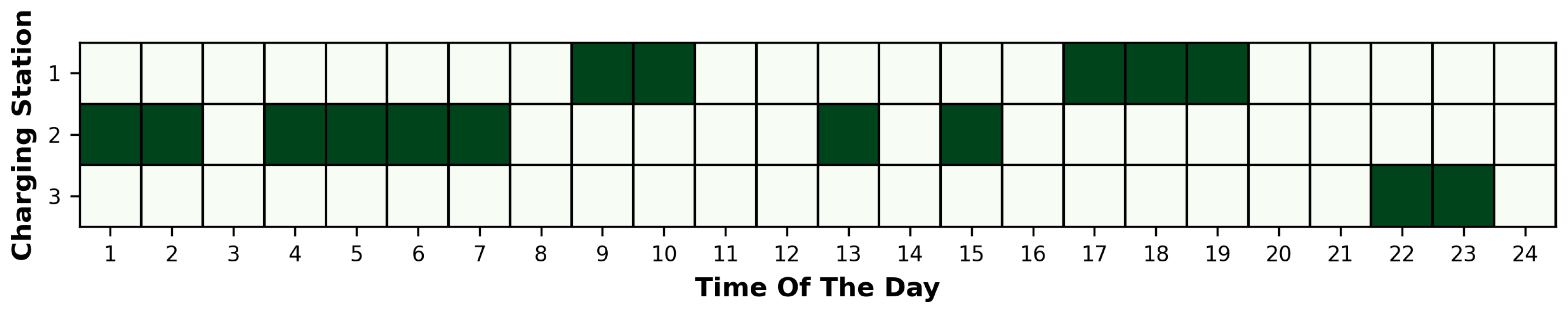
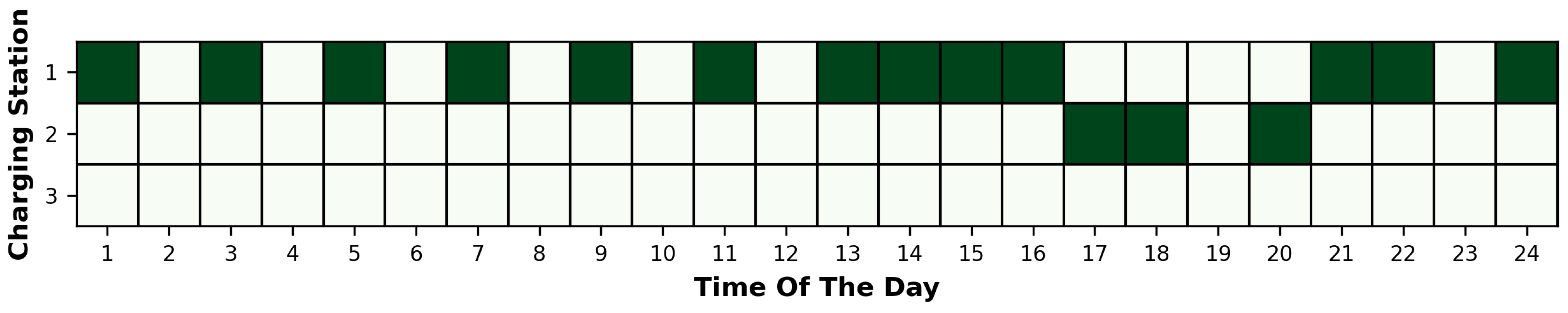
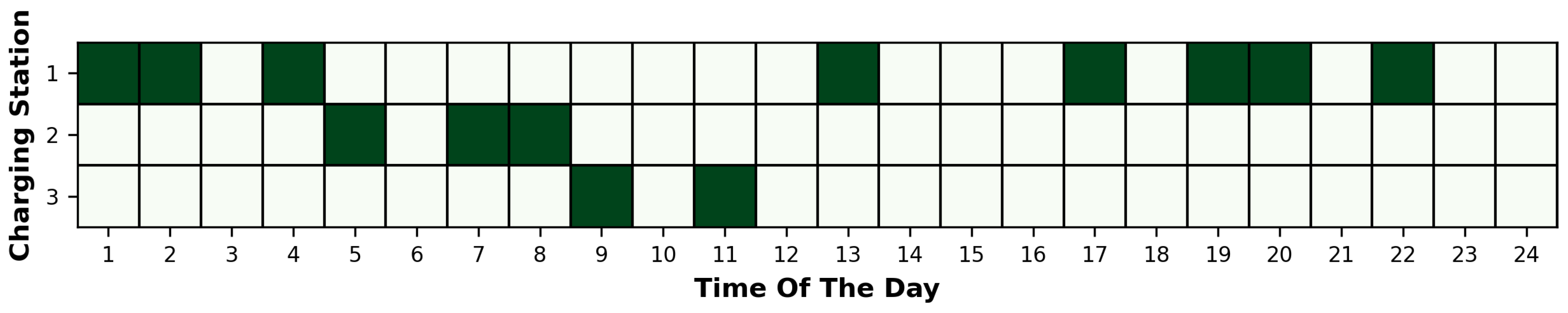
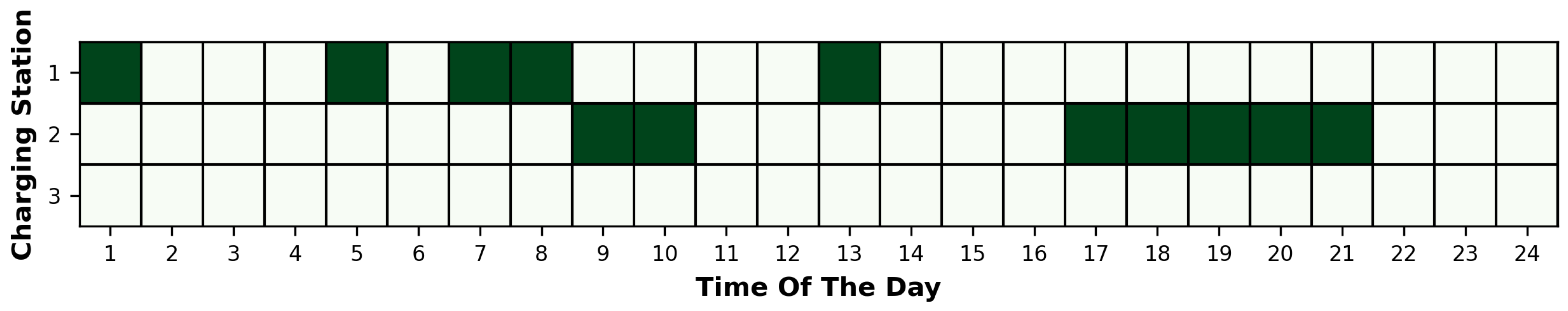
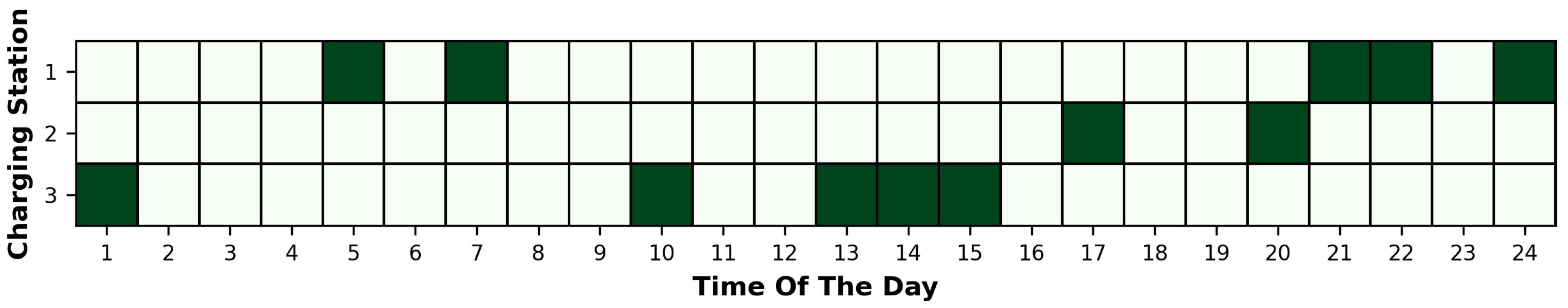
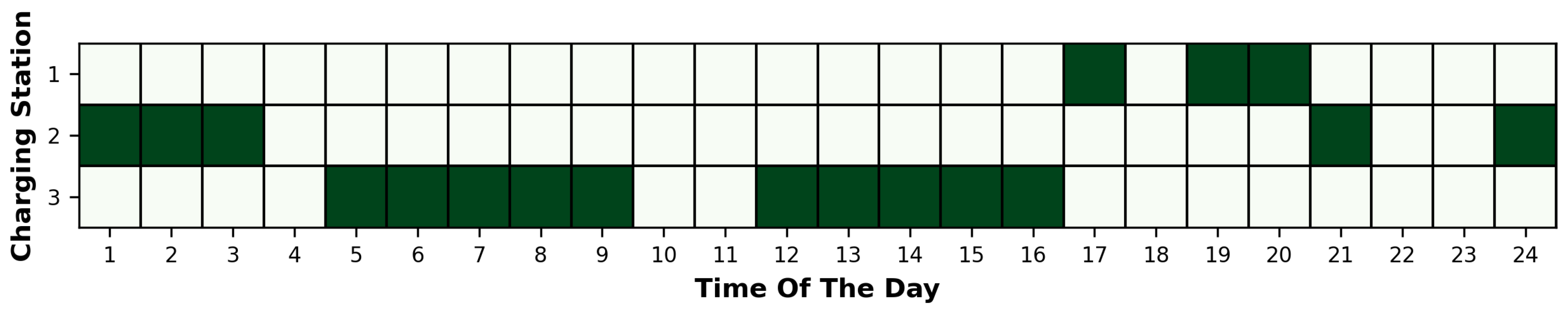
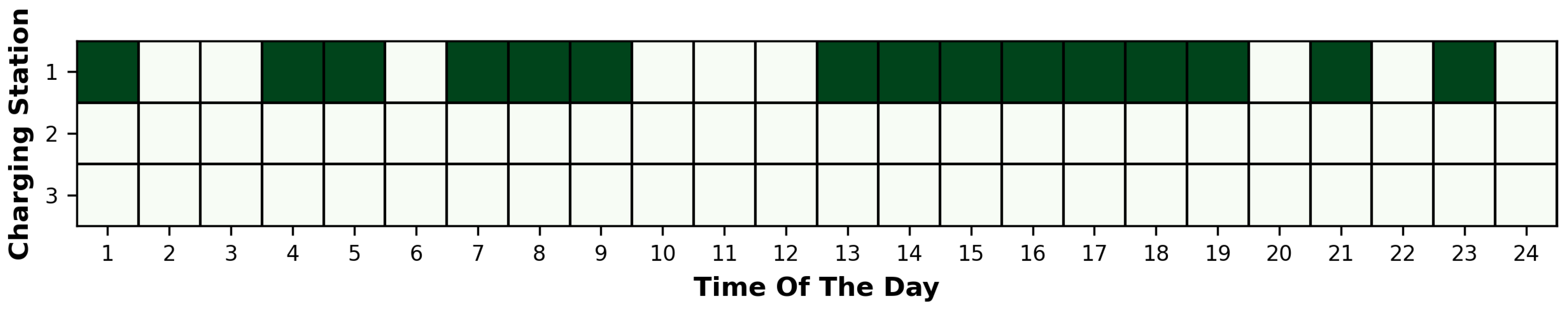
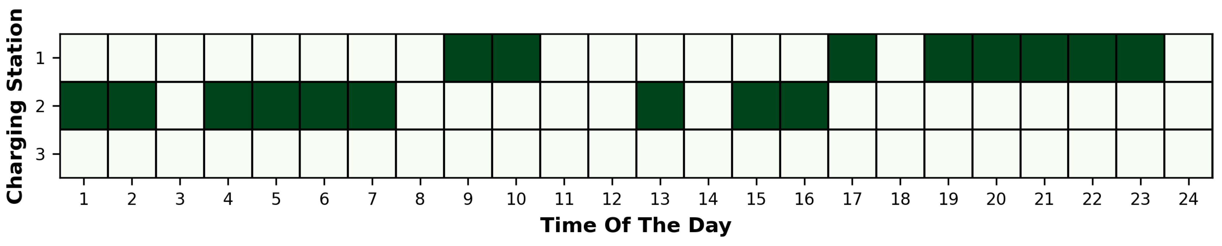
Figure 9, Figure 10, Figure 11, Figure 12, Figure 13, Figure 14, Figure 15, Figure 16, Figure 17, Figure 18, Figure 19, Figure 20, Figure 21, Figure 22 and Figure 23 exhibit heatmaps representing the connection patterns of electric vehicles. These heatmaps employ color variations to visually represent data values, facilitating a deeper understanding of the locations/events within the dataset and guiding the viewer to areas of interest. In this model, the heatmap indicates each EV’s connection to specific charging stations at various hours of the day. For example, in the first heatmap, the green color in the cell at row 1 and column 1 signifies that the EV is connected to the first charging station. The blank white spaces represent periods when the EV is not connected to any charging station.

5.3. Julia Programming and System Parameters

As a high-level programming language, Julia is renowned for its accessible syntax, significantly simplifying the process of code reading and writing for users. Moreover, it is designed with a dynamic type system and employs just-in-time (JIT) compilation, which lends itself to rapid code execution. This enables it to produce a performance comparable to that of statically compiled languages such as C and FORTRAN, making it particularly beneficial for optimizing mathematical models on a large scale, which necessitates fast computation.

Julia has built-in optimization libraries such as JuMP (Julia for mathematical programming) and Convex.jl. These libraries facilitate the straightforward implementation of optimization models. JuMP provides the convenience of specifying optimization problems using an intuitive, mathematical syntax, while Convex.jl offers a comprehensive toolset for resolving convex optimization problems.

Another essential feature of Julia is its design for interoperability with other languages. This allows it to easily integrate with pre-existing software systems, a feature particularly advantageous for optimization models that rely on data from diverse sources or need to be embedded within larger software systems. Collectively, these characteristics—high-level syntax, rapid performance, inclusive optimization libraries, and interoperability—render Julia a preferred choice for optimization modeling. This study employs the Gurobi.jl optimization library with the high-level JuMP package to implement the optimization algorithm.

In reference to Figure 1, the microgrid model comprises seven solar units, four wind units, three charging stations, two converters, and eleven transmission lines. The objective function yields an output in the form of binary variables—Is, Iw, Il, Ichs, Ic—which indicate the continued existence of each specific unit over the subsequent ten-year period.

Under normal operating conditions, the parameters are defined as follows: solar power (Ps) is 80 KVA, wind power (Pw) is 100 KVA, the charging power of each electric vehicle (EV) (Pch) is 40 KVA, the V2G power of each EV (PV2G) is 40 KVA, the converter capacity (Pc) is 250 KVA, and the maximum energy stored in each EV is 100 KVA. The demand is anticipated to increase annually by 2 percent over the coming decade.

Power flow constraints within the model are dictated by line parameters, such as conductance and susceptance. These are determined through calculations based on resistance, inductance, and line length. The costs associated with each solar, wind, converter, and charging station unit are established in relation to their respective capacities.

6. Results and Discussion

6.1. Normal Operating Conditions

It is presumed that EVs are incorporated into the system for typical operating conditions. Figure 24 presents a snapshot of the model output for the first year, delineating the variation over all the 24 h of a single day type. The highest outputs are solar—270 KVA, wind—250 KVA, charging power of EVs—150 KVA, and V2G (vehicle-to-grid) power—170 KVA. These combined sources satisfactorily meet the system’s peak demand of 450 KVA.

The plot indicates that when solar availability dips, particularly from 1 to 5 a.m. and 9 to 11 p.m., EVs supplement the grid with energy. Conversely, the EVs charge primarily during peak solar availability, i.e., from 7 a.m. to 5 p.m. This pattern underlines the pivotal role of electric vehicles in the microgrid model. Various contributions can be distinguished: the green line signifies solar output peaking between 9 a.m. and 2 p.m., the orange line represents wind output peaking from 1 am to 4 a.m. and 9 p.m. to 11 p.m., the blue line tracks EV charging, and the brown line depicts V2G power, indicating energy supplied back to the grid by EVs. The binary variables Ich and Iv2g for charging and V2G power define the ideal times to charge the EVs and return energy to the grid to meet demand.

6.2. In the Absence of Electric Vehicles

For the second scenario, where EVs are excluded from the model, the output resembles Figure 25. The absence of V2G power due to the non-inclusion of EVs results in the demand surpassing the capacity of the available units (solar and wind).

The plot’s red line depicts the total demand served, and the blue line represents the required demand. It becomes evident that when solar availability is minimal, i.e., between 1 a.m. and 4 a.m., and 9 p.m. and 11 p.m., the demand served falls short of the requirement.

6.3. For Changes in Parameter Values

In the third case, Figure 26 demonstrates the effect of parameter changes such as the installation costs of solar and wind units and penalty factor. Suppose the installation costs of solar and wind units increase, and the penalty for not serving the load decreases. In that case, the solar and wind outputs become non-optimal, i.e., they do not follow a specific pattern. This contrasts with the output in Figure 24, where solar and wind provides a consistent output for a defined period, and in Figure 26, where the solar and wind output curves are non-optimal.

6.4. For Different Scenarios/Uncertainties

In the fourth case, the “output plot for uncertainties” (Figure 27) encapsulates the effect of uncertainties inherent in solar and wind generation. The fluctuating nature of these renewable sources leads to wide-ranging outputs. Incorporating these uncertainties into the model facilitates a more realistic depiction of the energy system.

The figure exhibits the optimized solar and wind output; however, it is clear that the served demand fails to meet the required demand. Capacity expansions in solar or wind units can be contemplated to remedy this deficit and fulfill the desired energy needs. By enhancing the capacity of these renewable sources, the energy generated can better align with the energy demand, thereby ensuring a more reliable and adequate power supply.

6.5. Sensitivity Analysis

6.5.1. Changes in the Total Demand

The sensitivity analysis plot in Figure 28, entitled “impact of increase in demand on total installation cost”, exhibits that as microgrid demand grows over the next decade, so does the total installation cost. This is attributable to the need for additional infrastructure—solar panels, wind turbines, charging stations, or transmission lines—raising the overall installation expenses.

Thus, it is imperative to account for anticipated demand growth when estimating the total installation cost for the microgrid system.

6.5.2. Changes in the Solar Installation Cost

Figure 29 represents the relationship between the total installation costs of a microgrid (represented on the x-axis) and the associated solar unit installation costs (represented on the y-axis). Both costs are measured in millions of US dollars. As we move along the x-axis from left to right, we see how the cost of solar unit installation changes with the increasing total cost of microgrid installation. As the solar unit capacity considered in this model is 80 KVA, this unit’s cost is assumed to be USD 150,000. For a sensitivity analysis, various values ranging from 50 percent of 150,000 and 150 percent of 150,000 are considered, and the corresponding total installation cost is observed.

6.5.3. Changes in the Wind Unit Installation Cost

Figure 30 represents the relationship between the total installation costs of a microgrid (represented on the x-axis) and the associated wind unit installation costs (represented on the y-axis). Both costs are measured in millions of US dollars. The model’s original wind unit installation cost is USD 280,000 for a 100 KVA wind unit. If this value changes from 50 to 150 percent of 28,000, then the y-axis represents the total microgrid installation cost.

6.5.4. Changes in the Charging Station Installation Cost

Figure 31 represents the relationship between the total installation costs of a microgrid (represented on the x-axis) and the associated charging station unit installation costs (represented on the y-axis). Both costs are measured in millions of US dollars. As the charging station unit capacity considered in this model is 100 KVA, this unit’s cost is assumed to be USD 3000. It is observed that with a 10 percent change in charging station installation cost, the total cost increases by around 5 percent. So the impact of the cost of the charging station on the total installation cost is less than the effects of the increase in the solar unit and wind unit installation costs. This means that the installation of a new charging station is more economical compared to the installation of a renewable unit.

7. Conclusions

In conclusion, this work presents the planning of a zero-carbon-emission hybrid AC/DC microgrid, utilizing an optimization technique that yields binary variables to determine a ten-year installation plan for renewable energy sources, including solar, wind, converters, transmission lines, and charging stations for electric vehicles. The optimization model effectively minimizes the overall cost of microgrid installation and operation while accounting for various constraints. This research presents the strategic planning of a hybrid AC/DC microgrid to achieve zero carbon emissions. It applies an optimization technique that employs binary variables to formulate a decade-long installation plan for renewable energy infrastructure, such as solar and wind installations, converters, transmission lines, and charging stations for electric vehicles. The devised optimization model effectively minimizes the cumulative cost of microgrid installation and operation, adhering to a set of constraints.

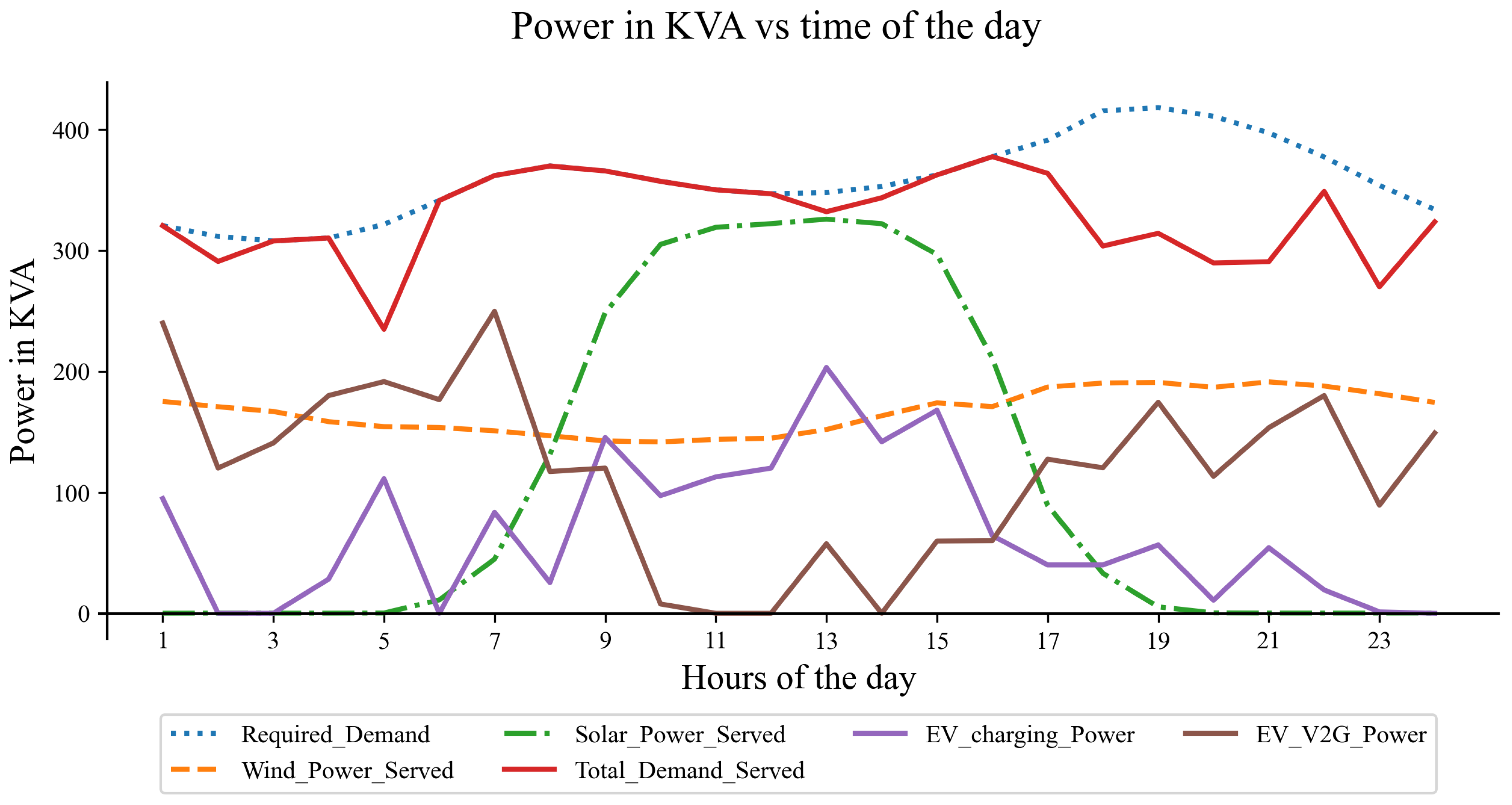
Integrating electric vehicles into the AC/DC microgrid has shown that the system’s generated energy can be optimally distributed both spatially and temporally thanks to the implementation of vehicle-to-grid (V2G) technology. This temporal energy distribution is highlighted in the first case study, as discussed in the ’Results and Discussion’ section. Here, the incorporation of electric vehicles and the use of V2G technology sufficiently meet the energy demand without incurring penalties, thus relieving the pressure on renewable energy sources. According to this case study plot, from 1 a.m. to 5 p.m. and 10 p.m. to 12 a.m. each day, the total required demand of the system is around 320–350 KVA. Out of this, the demand served by wind units is around 220 KVA. As solar power availability is negligible during this time, the remaining 130 KVA of required demand is served by the V2G technology of electric vehicles. This demand response management is the most important contribution of V2G in this case.

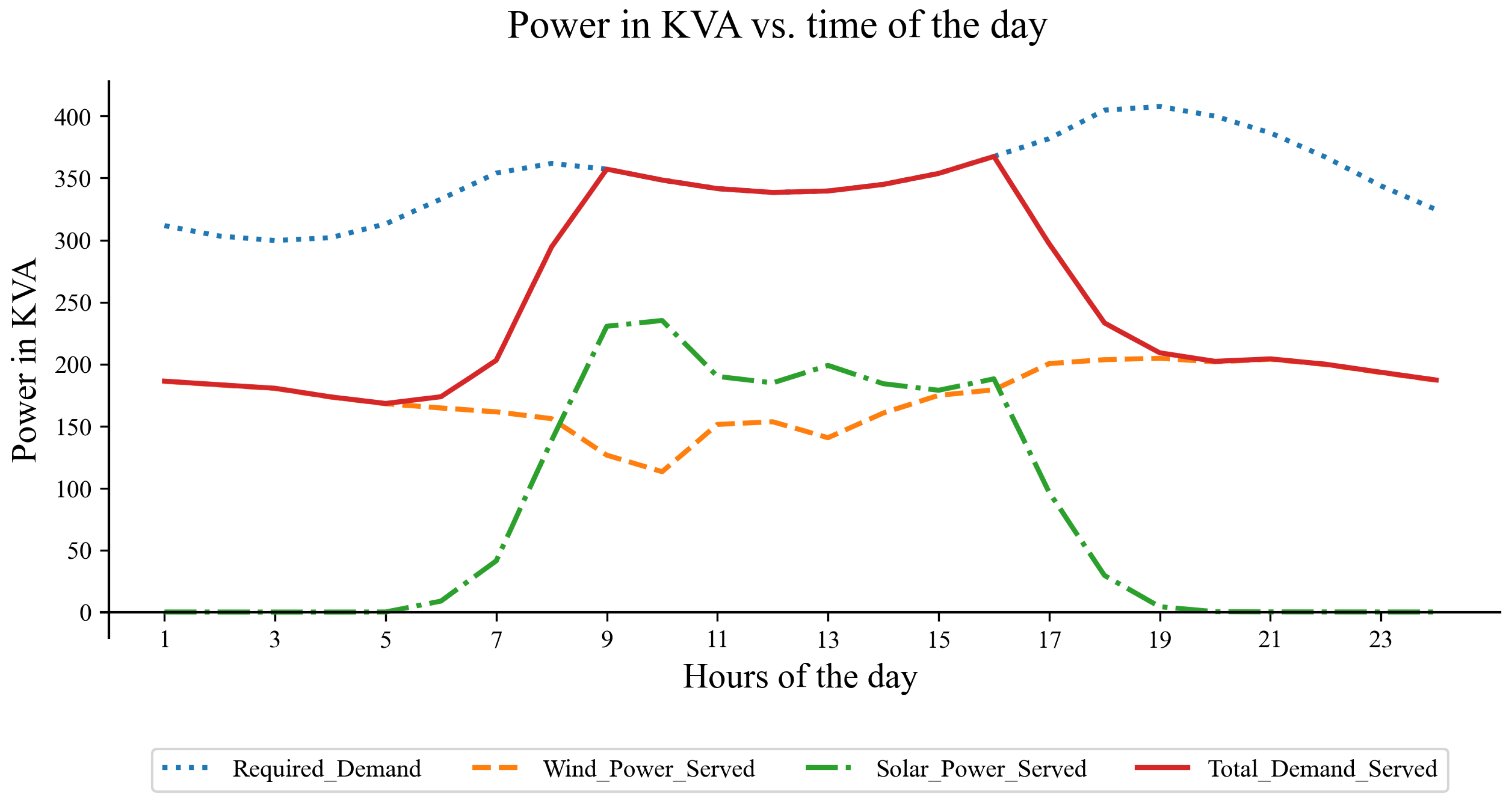
The second case study, which excludes electric vehicles from the model, demonstrates that the lack of their contribution results in unserved demand during specific periods, thereby attracting penalties. This underscores the substantial role of electric vehicles and V2G technology in optimizing resource use and satisfying energy demand within the microgrid.

To enhance the model’s robustness and realism, uncertainties inherent in solar and wind generation have been taken into account by employing various scenarios. The raw data on solar irradiance and wind flow, sourced from the CAISO website, are processed and normalized using clustering as a machine learning algorithm. This method simplifies computational complexity while preserving data authenticity.

The optimization model uses the Julia programming language and the Gurobi optimization library. It is noteworthy that the current model is static, operating on extrapolated and stationary input data. For future improvements, dynamic data inputs could be integrated, specifically concerning the travel patterns of electric vehicles and their charging needs. Furthermore, the model’s sophistication can be escalated by introducing an incentivized pricing scheme for electric vehicle integration.

Overall, this work offers a model that echoes real-world resource planning scenarios, laying a robust groundwork for tackling more intricate resource management challenges. Future research extensions can concentrate on incorporating dynamic data inputs, refining pricing models, and addressing additional complexities related to resource allocation and management.