Regression Models and Shape Descriptors for Building Energy Demand and Comfort Estimation

Abstract

Optimal building design in terms of comfort and energy performance means designing and constructing a building that requires the minimum energy demand under the given conditions while also providing a good level of human comfort. This paper focuses on replacing the complex energy and comfort simulation procedure with fast regression model-based processes that encounter the building shape as input. Numerous building shape descriptors were applied as inputs to several regression models. After evaluating the results, it can be stated that, with careful selection of building geometry describing design input variables, complex energy and comfort simulations can be approximated. Six different models with five different building shape descriptors were tested. The worst results were around R² = 0.75, and the generic results were around R² = 0.92. The most accurate prediction models, with the highest level of accuracy (R² > 0.97), were linear regressions using 3rd power and dense neural networks using 1st power of inputs; furthermore, averages of mean absolute percentage errors are 1% in the case of dense neural networks. For the best performance, the building configuration was described by a discrete functional point cloud. The proposed method can effectively aid future building energy and comfort optimization processes.

1. Introduction

Since the early 1970′s, but especially after 2000, within the field of building energy, comfort, and environmental design optimization (BECEDO), there has been a search for the most suitable combination of input design variables (DV) to reach the desired level of BECEDO performance, i.e., output parameters. In architecture, automated coupling between mathematical optimization algorithms and numerical building physics simulations utilizes a large number of calculation iterations (that are manually unmanageable) to provide the highest proximity to the given objective function in the search space. By manipulating various input design variables, subject to diverse constraints, the minimum or maximum value of the cost or fitness of an objective function is sought [1].

Our research framework aims to create an artificial intelligence-based model that supports the design of optimal building structures with a focus on sustainability. Specifically, the model enables the design of multi-objectively optimized buildings in terms of energy and comfort performance as well as environmental impact (Life Cycle Assessment, LCA). To achieve this, two critical factors must be considered: (1) understanding the effects of input design variables on the output variables is crucial for making later decisions regarding input variable combinations; and (2); the acceleration and substitution of complex, high-resolution white-box simulations makes it possible to save significant building physics modelling and calculation resources and facilitates the handling of large search spaces.

This research deals with the latter (2) strategic measures-the rationalization of the simulation framework. Building climate, energy, and LCA simulations support the development of decreased energy demand by maintaining a high level of indoor comfort quality with minimized environmental impact. Using the energy, comfort, and environmental results, the selection of the optimal case(s) is extremely resource intensive in both calculation duration and expert working hours. This modelling, assessing, and analysis demand significantly increases as the number of buildings and input design parameters increase. By replacing the complex simulation procedure with a regression technique, the determination of optimal building input design parameters and, thus, the planning of energy, comfort, and environmentally efficient buildings can be significantly sped up. The task of regression models is to approximate the unknown relationship between descriptive and dependent variables or to simplify known but complex relationships. Such processes are used in almost all fields of science; therefore, their application is not new in architecture or energy optimization.

Peña-Guzmán and Rey [2] used multiple linear regression models to estimate the future development of residential electricity consumption with an accuracy of R² above 0.93. Mehedintu et al. [3] used polynomial and autoregression models in their study to estimate the ratio of total energy used in the EU to energy consumption from renewable sources. The R² point was used to measure efficiency, with an accuracy level of over 0.91. Mohammed et al. [4] approximated the energy demand of school facilities, whereas 350 teaching and 35 testing data points were applied to create the linear regression with a model accuracy of over 90%. Another study presents an emulator-based approach with an optimization algorithm for building energy simulation models for calibration purposes [5]. Multiple Linear Regression (MPL) and Gaussian Process (GP) were examined with an R² above 97% prediction accuracy, and the meta-models used could increase validation speed and reliability with a small amount of training data from white-box simulation results.

Dudek used [6] a Random Forest (RF) of Regression Trees (RT) to forecast the short-term energy demands of countries to support resource planning. Real data was collected between 2012 and 2014 in Poland, Great Britain, France, and Germany, and RF forecasts were the most accurate compared to other data-driven statistical and Machine Learning (ML) models (MultiLayer Perceptron MLP, Support Vector Machine, long-short term memory, fuzzy neighborhood model, etc.). Vardhan et al. [7] also compared energy demand forecasting for a city using different ML models (Linear Regression (LR), Decision Tree (DT), SVM, and Neural Network (NN) and found that the best performing model was the DT, with R² = 0.85, slightly higher than R² = 0.82 of the NN. Park et al. [8] used a Gradient Boosting (GB) Regression Tree for short-term forecasting of the outputs of a wind farm on Jeju Island. Moreover, they found their monthly and seasonally trained forecasting GBRF model to yield the best results.

Artificial neural networks (ANN) [9], consisting of a feedforward multilayer neural network with a back-propagation technique, predicted either heating energy use or indoor temperatures at the individual or building stock level with an R² of >0.93. Building heating energy demand in residential buildings was assessed via ANN (R² 0.908) in a further model development [10]. Zou et al. [11] tested diverse ANN models, which accelerated the optimization calculation by approximately 2570 times compared to traditional simulation-based optimization methods. The R² values settled above 0.965 in the ANN model version with the best predictive ability. [12] sought the impact of using different machine learning techniques on the accuracy of predicting building energy usage over a rolling horizon framework and how forecasting errors can be reduced using data segmentation. The Clarendon building of Teesside University served as a specific building example, and the energy use dataset for the year 2018 contained energy usage as well as sensory data of internal and external temperatures in a 15 min resolution. Machine learning techniques such as linear regression (LR), polynomial regression (PR) using six degrees of polynomial regression, support vector regression (SVR), and artificial neural networks (ANNs) were considered there. They claim a significant reduction in the mean absolute percentage error (MAPE) when segmented building (weekday and weekend) energy usage predictions were compared to unsegmented monthly predictions. They also suggest that the training data should follow historical data from the same season. Further, the study showed that when working with limited datasets with few inputs and outputs, SVR can outperform ANN. Elsewhere, [13] developed a GIS-based procedure for estimating the energy demand profiles of urban buildings. They used dynamic simulations of a set of Building Energy Models adopting different energy-related features. The simulation models considered thermal zones. They considered simulated hourly energy density profiles. The building stock of Milan, Italy, served as an illustration, and the results were validated with the data available from the annual energy balance of the city. In another study, [14] also considered different machine learning techniques to predict building energy needs and to circumvent energy simulations. They compared Linear Regression, Support Vector Machine, Random Forest, and Extreme Gradient Boosting (XGB) results. Mean Absolute Error (MAE), Mean Squared Error (MSE), and R² score served, besides the computational time, as evaluation metrics for the considered models. The numerical model of a winery building close to Bologna, Italy, served as an illustration and the basis of the used dataset. 11 user-inserted features, including the building orientation, wall resistance, and wall conductivity, were considered variables, and 5150 simulations were run. In conclusion, it was stated that machine learning methods offer efficient and interpretable solutions. XGB provided the best results in terms of MAE, MSE, and computational time.

Although in the previously presented publications machine learning methods were used to surrogate energy simulations, these models were created for specific buildings and did not consider the building shape configuration as input.

Based on the examination and comparison of scientific results [15], we stated that building geometry has a significant effect on the annual energy demand; hence, energy-efficient planning and optimization should also be extended to involve the building shape in the form of input design parameters. Building geometry decisively influences the seasonal operation expenses, and 60–80% savings in energy consumption, as well as approx. up to 80% of LCA improvements, were already assessed [16,17,18,19]. However, despite the significant influence of shape on the energy performance of a building, during the energy optimization of the built environment, it is not generally considered, or only to a small extent, relying instead on intuition, tradition, and professional experience of the designer. Scientific studies focus mainly on easily definable design variables (DVs) such as heating, ventilation, and air conditioning (HVAC) system parameters, energy management system values, and system operation data, and only a few attempts have been made to integrate geometry-related DVs into the BECEDO [19,20,21,22]. In addition, other literature [15,19] demonstrates that when prioritization of building geometry design variables (BGDVs) in a consecutive optimization process occurs, significant savings can be achieved in subsequent passive and active system design and construction, as well as operational costs. In other words, BGDV optimization must be followed up with engineering DV considerations such as passive (architectural) and active (building services) systems, energy supply system-related DV-s, as well as operation strategy solutions like developing a multi objective optimization procedure to enhance the efficiency of heat pump heating systems through energy optimization [23] by A. Nyers and J. Nyers. The current study carefully analyses selected BGDVs in the regression process.

We previously demonstrated that complex and computationally intensive energy simulations, which calculate the building shape configuration (hereinafter configuration) describing BGDV-s, can be replaced by a linear regression procedure [24,25]. Here, the target is to examine the applicability of regression procedures that are more advantageous than the presented linear regression and to select and elaborate a specific regression model to support the solution of building simulation-based optimization tasks. Note that the configurations extensively influence the final energy demand and comfort levels. Therefore, the study involves dynamical configurations of a specific family house class of problems and not only one building shape. During the investigation, regression models were created to indirectly estimate the expected annual heating, cooling, and lighting energy demands, as well as the thermal and visual comfort of variations in the building. Under the framework of the experiments, where necessary, the nonlinear regression ability was improved by increasing the correlation/interdependency of the input variables, and then the learning time and accuracy of the models were compared. The advantage of the researched regression model is not only the higher accuracy but also, by selecting a suitable, reasonable regression technique, the model’s capability to implement the BGDV-s (configuration describing parameters) is of utmost importance, along with the flexibility, adaptability, and applicability of the model in further investigations.

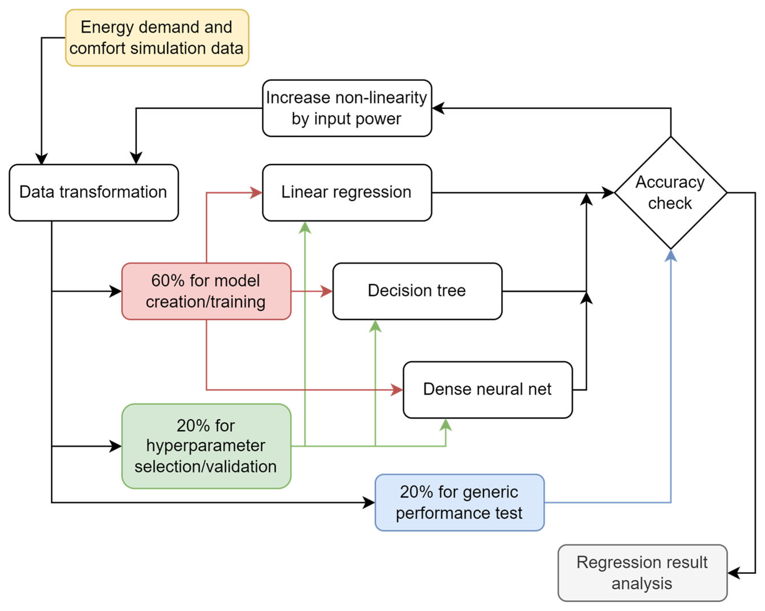
The research applied the following structure: Following the Building Energy demand and comfort simulations section, the regression models are applied; then there is a description of how the models are evaluated and a check for accuracy; then a required power of inputs is selected; then the configuration descriptors are discussed, which is followed by a detailed analysis of the results (Figure 1).

2. Building Energy Demand and Comfort Simulations

To build the hypotheses and create building case versions, 5010 data samples were created for dynamic indoor climate and energy simulations via IDA ICE software. To keep the simulations and their regression in a controlled environment, specific building configurations were used. In the current experiment, a generic detached house was examined, and, as a reference, variables from an existing award-winning Active House were applied [26]. To prepare the simulation calculations, architects and mathematicians developed a huge number of configurations for testing optimal building geometries [25]. The investigated building configurations were made of six building blocks of the same size with all the necessary functional spaces for a residential building (living room, kitchen, bedroom, etc.). From these six building blocks, for a 5 m × 5 m × 3 m space, 201,359,550 different configurations were possible. To provide for building configurations that can be built and function as residential houses, specific architectural rules were applied to eliminate incompatible configurations. This resulted in 167 different detached house configurations.

These configurations needed to be equipped with architectural design properties (wall-window ratio, main facade orientation) as well as engineering properties (structures and materials, mainly related to thermal insulation and thermal capacity, heating, cooling, and ventilation infrastructure), and components. During dynamic thermal simulations, based on data from the ASHRAE IWEC weather database over multiple years, the annual energy (heating, cooling, and artificial lighting in kWh/a) and comfort data of the buildings were calculated. Thermal comfort performance was assessed in the form of the occupancy time ratio of annual operations, where the operative temperature is based on the thermal comfort category of II (B) according to EN 16798-1 and ISO 7730. The simulation model creation procedure is described in [24]. The visual comfort is modelled by calculating the daylight factor (DF) of the complete net floor space and assessing the area ratio that provides a DF value above the 1.7 threshold, according to EN 17037. The following DV-s were set as complementary parameters to the configuration descriptors (BGDV-s):

Engineering DV-s

• Two alternating building envelope structures with different thermal insulation were applied (U_wall = 0.24 and 0.11 W/m² K; U_floor = 0.28 and 0.17 W/m² K; U_roof = 0.17 and 0.14 W/m² K; U_glazing = 1.0 and 0.7 W/m² K;).
• Three different wall-window ratios (WWR) were used on the main façade of each building model: 30%, 60%, and 90%.

BGDV-s

• Configuration parameters and representation (see later section “Configuration descriptors”)
• Main façade orientation in the significant solar exposed positions is E, SE, S, SW, and W.

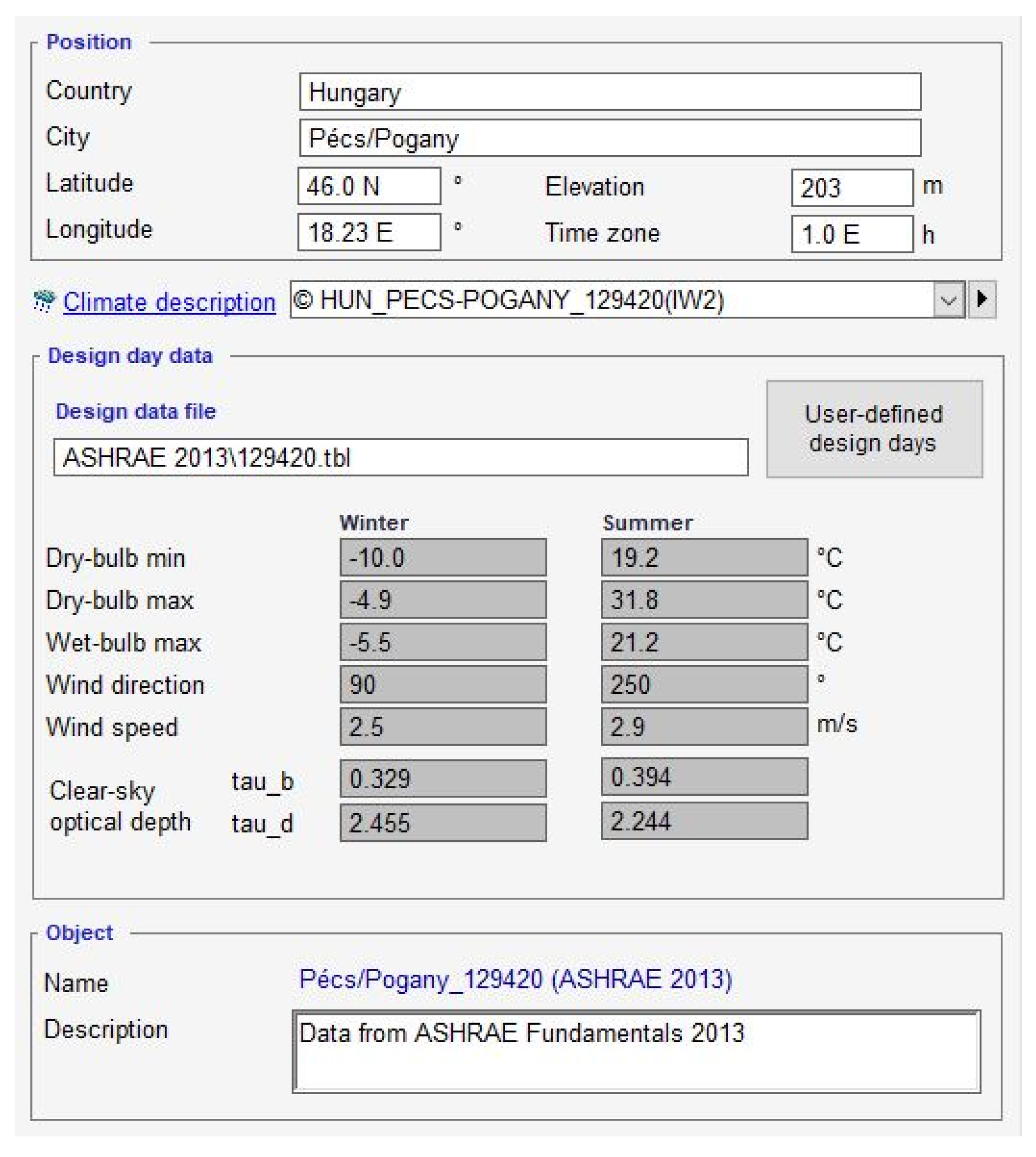
The location of the simulations is Pécs-Pogány (South of Hungary), whereas the data is derived from ASHRAE Fundamentals 2013, depicted in Figure 2.

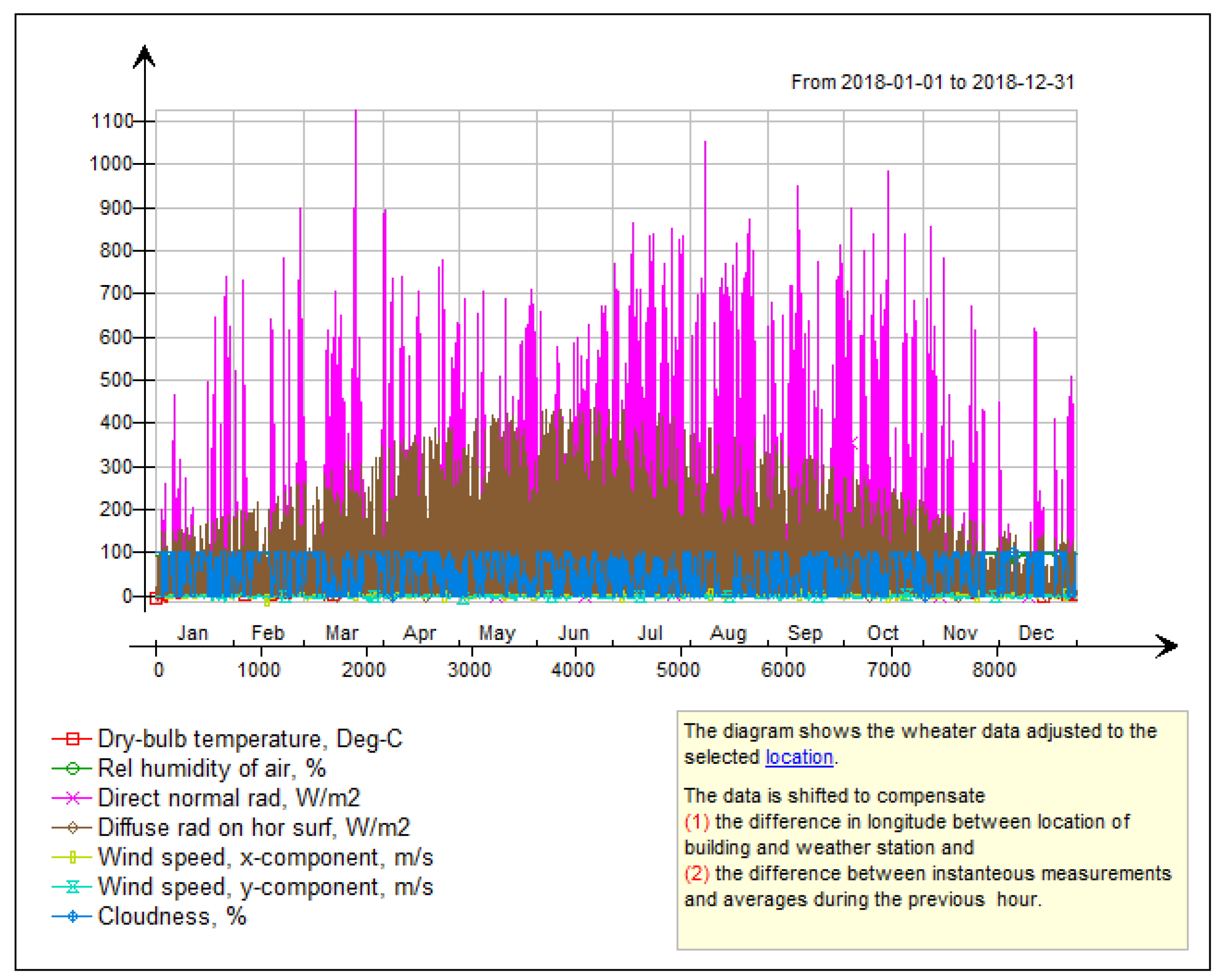
• The climate file applied in the dynamic calculations (IDA ICE 4.8 SP2 of EQUA Simulation AB, Stockholm, Sweeden) is derived from the ASHRAE IWEC2 Weather File for PECS-POGANY. (c) 2011 American Society of Heating, Refrigerating, and Air-Conditioning Engineers, Inc., Atlanta, GA, USA. This meteorological database possesses a whole year time interval in hourly-averaged value resolution in external air temperature, relative humidity, direct and diffuse solar radiation on a horizontal plane surface, wind, and cloudiness circumstances. The used climate file is demonstrated in the following graph (Figure 3):

Figure 3. The climate database used in the simulated building model versions has the 7 main meteorological parameters of dynamic building comfort and energy simulations.

Figure 3. The climate database used in the simulated building model versions has the 7 main meteorological parameters of dynamic building comfort and energy simulations.

Please note that the following type of HVAC system was used:

Ventilation, heating, and cooling: Mechanical ventilation air volume flow rate is set to 2 L/sm² to provide the necessary air change; 100 W/m² heating and 200 W/m² cooling power are modelled in each space to cover a comparable thermal energy demand, whereas the COP and EER values were kept at 1 (hence, at least in the research phase, no efficiencies were considered).

This was not considered a design variable since the main target of this investigation is the effect of building configurations on annual energy demand and comfort. Obviously, different HVAC systems would result in different annual energy demands and comfort values. How different HVAC systems affect the final rank of the configurations and whether different HVAC systems should be applied to various configurations will be investigated in the future.

The main results of the simulation for the 167 building configurations multiplied by the previously mentioned variations in parameters (a total of 5010 case combinations) are detailed in

Table 1. Simulation results.

Data	Minimum	Maximum	Interval
Heating energy [kWh/a]	5486	15,098	9612
Cooling energy [kWh/a]	99	3261	3162
Lighting energy [kWh/a]	915	3008	2093
Thermal comfort [% of yearly occupancy time]	6	69.36	93.36
Daylight factor [% of net floor area]	14	70	55.87

Note that experimental data from real buildings may verify and validate the accuracy of energetic and comfort simulations. Simulation data were generated by validated, accepted, and widely used simulation software (IDA ICE); therefore, simulation results are accepted as valid data. Furthermore, because the simulated building specifications were not built, no experimental data could be collected. Nevertheless, the method presented hereinafter concentrates on the substitution of complex, time consuming, energetic, and comfort simulation; instead, the evaluation of the presented surrogate methods is described in Section 4, but the validation of simulations is not within the scope of the present method.

. As seen, up to 2/3 of the total energy demand (the sum of heating, cooling, and lighting energies below) is dominated by the energy required for heating; therefore, our examinations are initially focused on these values.

3. Regression

Regression calculation [27] is a frequently used statistical method in which the type and, more likely, the parameters of the dependency between inputs and outputs are specified.

Ground truth function:

$$y=f\left(\overline{X}\right)$$

The function $y$ is given by a set of N ($\overline{X}$, $y$) sample pairs:

$$S=\left\{\right({\overline{X}}_1, y_1), ({\overline{X}}_2, y_2), \dots , ({\overline{X}}_N, y_N)\} \mathrm{where} \left|S\right|=N$$

Create a hypothesis $h\left(\overline{X}\right)$ that is close enough to the ground truth. When E is a distance (or Error) function, close enough is specified in (1).

$$E\left(y,h\left(\overline{X}\right)\right)\le \epsilon \epsilon is the acceptance criterion$$

(1)

A generally used error is the sum of the squared errors at the sample points described in (2).

$$E=\sum _{i=1}^N{\left(y_i-h_i\right)}^2$$

(2)

3.1. Linear Regression

Linear regression [28] is a special case of generic regression, when the dependent variable is created as a linear combination of the input variables, based on the Taylor series of (3).

$$y={\beta }_0+{\beta }_1{x}_1+\dots +{\beta }_n{x}_n+\epsilon$$

(3)

$$h\left(x\right)=\tilde{y}={\beta }_0+{\beta }_1{x}_1+\dots +{\beta }_n{x}_n$$

(4)

$$\epsilon =y-h\left(x\right)=y-\tilde{y}$$

(5)

where y is the dependent variable, x₁…x_n are the inputs, β₀…β_n are the parameters of the linear regression model, h(x) of (4). is the hypothesis of the linear regression, $\tilde{y}$ is the estimated value of the dependent variable, and is ε of (5). is the error of the linear regression. With the introduction of $x_0$… $x_M=\overline{X}$ and ${\beta }_0$… ${\beta }_M=\overline{\beta }$, the formulation can be vectorized to (6).

$$h\left(\overline{X}\right)=\tilde{y}={\overline{\beta }}^T\overline{X}$$

(6)

The generally used method for model creation and computation of the parameters is the Least Squares method [29].

3.2. Non-Linear Approximation

The annual energy demand of detached residential houses is a non-linear function. Since the estimation of non-linear functions with linear regression is only possible with a high error, the application of a non-linear regression is required. To provide non-linearity, a multiplicative combination of input variables with a higher degree is utilized in the applied approximator polynomial [30]. These are called polynomial regression models. The difficulty of this method is that the specification of multiplicative combinations and their maximum power is part of model creation; however, an analytical solution does not exist for this problem. An estimation of the simulated annual heating energy demand for a detached house can be performed using a multivariate linear regression with an accuracy acceptable for architects [24].

To support non-linear approximation, a set of input variables is extended with new ones that strongly depend on the original inputs. Since the introduced variables do not carry new information compared to the original variables, they only change the nature of dependency, the dimensions of the search space, and the relative resolution of the input samples.

As mentioned earlier, the introduced inputs are multiplicative combinations of the original ones up to a predefined maximum power.

As an example, for input sets {a, b}

• maximum 2nd power combination: a, b, a², ab, b²
• maximum 3rd power combination: a, b, a², ab, b², a³, a²b, ab², b³

In general, the new size of the extended set of inputs, ${\tilde{M}}_P$ is described by (7).

$${\tilde{M}}_P=\sum _{k=1}^P{\overline{C}}_M^k=\sum _{k=1}^P{C}_{M+k-1}^k=\sum _{k=1}^P\frac{\left(M+k-1\right)!}{k!\left(M-1\right)!}$$

(7)

where M is the original size of the input set and P is the maximum power.

Table 2. Input extension of multiplicative combinations.

Input Set Size	Power (P)	Example {a, b}	Independent	Single	Set of 14	Coordinates	Point Cloud
$M=\tilde{M}$	1	2	3	1 + 3	14 + 3	18 + 3	75 + 3
${\tilde{M}}_2$	2	5	9	14	170	252	3081
${\tilde{M}}_3$	3	9	19	34	1139	2023	85,319

shows the size change of the specific input sets when extending up to the second and third powers of multiplicative combinations.

3.3. Decision Tree

Decision tree-based regression models [31] estimate the dependent variable by repeated examination of the descriptor variables, one at a time. The result of a classification-like method is a binary tree graph, shown in Figure 4.

The leaf nodes of the binary tree are the estimated values. The internal nodes of the tree are the questions of decisions; their outgoing edges point to the next decision or the selected outcome. The decision itself is a threshold check of a single input variable. The output is generated by going through the decision tree at all input points in the search space. The result, shown in Figure 5, is a discrete multiclass classification of the search space. The classes are the finally selected estimation intervals, o their special values.

That is, the decision tree recursively shares the search space into subspaces until it reaches the maximum level or further division is not possible or required. The output is the average of the outcome interval values. The key to decision tree generation is the specification of the parameters of internal nodes, thus the parameters of the decisions. In detail, this is the selection of the descriptor variable for the next search space division and its threshold value. In the case of decision tree regressors, the selections are based on maximizing the variance gain of the split. As shown in (8), this is measured by the average error difference of the parent subspace and its left and right subspaces.

$$gain=\frac{{error}_{parent}}{N_{parent}}-\left(\frac{{error}_{left}}{N_{left}}+\frac{{error}_{right}}{N_{right}}\right)$$

(8)

maximizing gain is indeed the minimization of the total variance of subspaces, as (9) shows:

$$argmin {error}_{left}+{error}_{right}$$

(9)

As stated earlier, variance is measured by the error of the approximation. The following error measures are applied:

L1 distance, metric-based Mean Absolute Error

$$MAE=\frac{1}{n}\sum _{i=1}^n\left|y_i-{\tilde{y}}_i\right|$$

(10)

L2 distance, metric-based Mean Squared Error

$$MSE=\frac{1}{n}\sum _{i=1}^n{\left(y_i-{\tilde{y}}_i\right)}^2$$

(11)

The characteristics of distance metrics, shown in Figure 6, have an influence on the solution of the variance minimization task. Please note that, while MAE is linear, MSE is exponential, which results in higher costs for the more distant values.

The benefits of applying decision tree-based regression models are (i) a greedy algorithm with low resource requirements, (ii) good estimation, and (iii) an interpretable model. The drawbacks are (i) non-robustness sensitive to changes in training data; (ii) the creation of an optimal tree is an NP-complete task; and (iii) a good chance for overfitting.

3.4. Dense Neural Network

This model is inspired by the nervous system and based on a computation model described in the universal approximation theorem [32,33].

As Figure 7 shows, the internal structure of a general regression network [34] contains independent processor units, which are organized into layers. The first layer is the input layer; it receives the input from outside the model and makes it ready for processing without changing. The last layer is the output layer, which applies the computation model universal approximation theorem to create an approximation of the ground truth function as an output. Between the input and output layers, any number (from 0 to hundreds) of hidden layers could be placed. The main task of hidden layers is to extract special descriptors that make the final estimation more effective. In dense networks, each layer is fully connected to the next layer. Full connection means that all elements in a layer are connected to all elements in the following layer. No other connections exist in dense networks. In Figure 7, x is the collection of input features, M is the number of input features, H is the number of neurons in hidden layers, and O is the number of neurons in an output layer, which must match the number of output variables. In regression tasks, O = 1, because the model estimates one single continuous value. In the presented example, the network has two hidden layers of the same size; however, the number and size of the hidden layers could differ based on the task to be solved.

A schematic description of the processor units is shown in Figure 8. The processor units, in other words, cells or neurons, first calculate the weighted sum of their inputs. In this sum, all inputs have their own weights. Then cell outputs are generated by activation functions, which use the weighted sums as inputs. In a dense neural net, in a layer, the same activation function is used in all cells but could also differ between layers. Any kind of function could work as an activation function; however, to support the operation of the training method, special functions are used.

In a simplified structure, when the network does not contain hidden layers and the output layer contains only one neuron with a linear activation function, the previously explained linear regression appears. However, when applying a multi-layer connection of processing units and non-linear activation, a non-linear regression could be solved without extending the input variable set. According to current science, there is no analytic method to specify the appropriate network structure. The selection of applied network architecture is based on statistical analysis and comparison of training, validation, and test results.

4. Evaluation of Models

For model creation and training, 60% of simulations were randomly selected. From the remaining 40%, which is unknown for the model, 20% were used for model validation (hyperparameter selection), and the last 20% were used to test the generic regression ability of the models. Model evaluation is based on evaluating the estimation of each output item one-by-one in the training and also in the test set. To measure and compare the generic performance of models, a single value measure is required. The accuracy of estimations is measured by the mean absolute error of (10) and the mean squared error of (11). The R² score [35] of (12) is frequently used in statistics and regression. This measure, explaining to what extent the variance of input explains the variance of output, is also used.

$$the {\mathrm{R}}^2=1-\frac{\sum _{i=1}^N{(y_i-{\tilde{y}}_i)}^2}{\sum _{i=1}^N{(y_i-\overline{y})}^2}$$

(12)

Here $y_i$ is the ground truth, ${\tilde{y}}_i$ is the approximation of ith sample value, $\overline{y}$ is the mean. The maximum value of the R² score is 1. Lower values mean worse performance and may also result in negative values. For model evaluation, in addition, to the previously mentioned mean absolute and squared errors, the mean of error in a portion of the estimated value (shown in (13)) and the mean of its absolute value (shown in (14)) are also used. These error types are called mean percentage and mean absolute percentage errors.

$$MPE=\frac{{\sum }_{i=1}^N\frac{(y_i-{\tilde{y}}_i)}{y_i}}{n}$$

(13)

$$MAPE=\frac{{\sum }_{i=1}^N\frac{\left|y_i-{\tilde{y}}_i\right|}{y_i}}{n}$$

(14)

For the mean, the variance (shown in (15)) and standard deviation were also calculated. The sigma of (16) could be used for spanning confidence intervals of the normal distribution.

$$Var=\frac{1}{N}\sum _{i=1}^N{\left({\tilde{y}}_i-\widehat{y}\right)}^2=\frac{1}{N}\sum _{i=1}^N{\left({\tilde{y}}_i-\frac{1}{N}\sum _{j=1}^N{\tilde{y}}_j\right)}^2$$

(15)

$$\sigma =\sqrt{Var}$$

(16)

5. Neural Network Hyperparameter and Parameter Specification

The hyperparameters of the proposed neural network are the parameters that are not included in the training process. The ReLU activation function of cells and the ADAM optimizer were selected based on a literature review. The number of training epochs (1800), the size of training batches (16), and the internal structure (number and size of hidden layers) are specified based on the grid search algorithm. For the hyperparameter selector validation procedure, as Figure 1 shows, 60% of the samples (5010 simulation results) were used to train the model, 20% were used for validation/hyperparameter selection, and the final 20% were used to measure general accuracy. All measurements were repeated 10 times with random initialization and a random sample split. The results show the averages of results from the same settings. The merged variance of 10 independent random initializations and a random train-validation-test split was around 1% of the mean absolute percentage error; therefore, the training sample selection has no significant effect on the accuracy of the result.

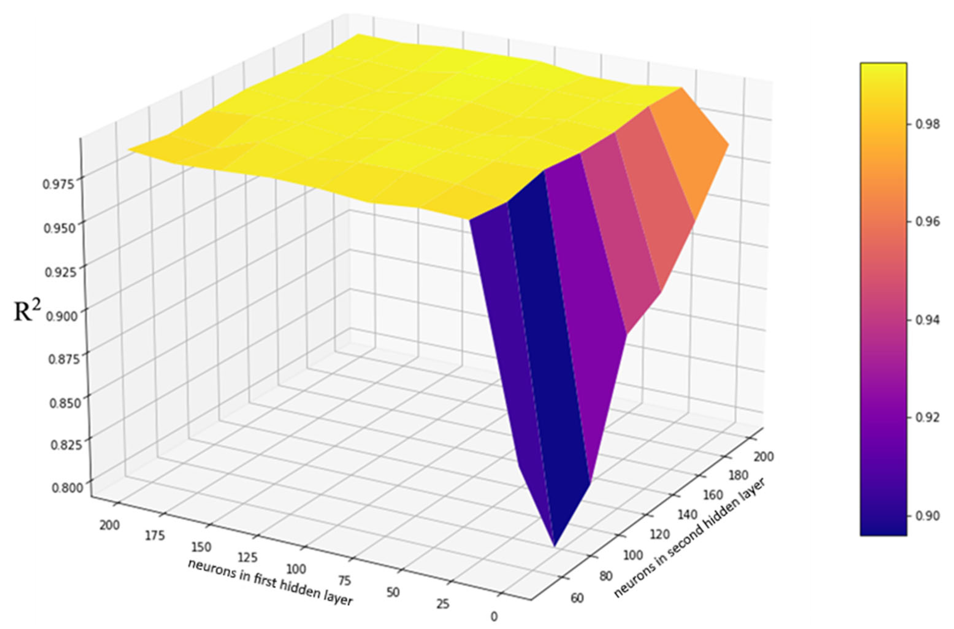
The most important and difficult-to-specify hyperparameter set is the internal structure of the network. Figure 9 and Figure 10 show the average R² scores of 10 models with the same structures using random initialization and random training sample selection. In Figure 9, the breakdown on the right of the graph is a decrease in accuracy resulting from networks with only one hidden layer with 50–200 neurons in it. The network structure was selected using the original set of input variables.

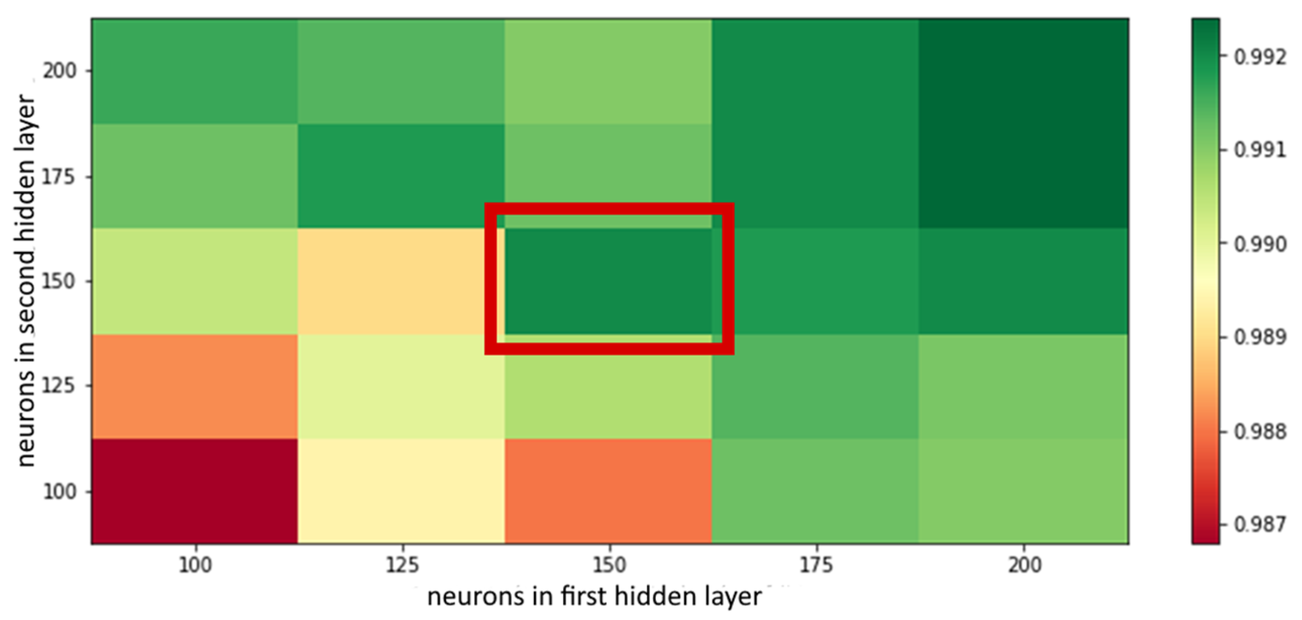
Because of the reduced accuracy of single-hidden-layer networks, the differences between two-hidden-layer networks are not visible. Therefore, Figure 10 only contains the R² score of two-hidden-layer networks with different numbers of neurons in each layer.

From Figure 10, the simplest network with high performance is the one in the center, marked with a red frame, when there are 150 neurons in each hidden layer.

Properties, that are specified as part of the training procedure are called network parameters; these are indeed the weights of connections between neurons in consecutive layers. According to the structure and operation of neural network initialization and training, many possible solutions can be obtained by repeating the initialization and training (including a random train-validation-test split). The run time of one network training, a.k.a. model creation, on an AMD Ryzen 5 processor with 32 GB of RAM and an NVIDIA GeForce GTX 1660 lasts approximately 600 s on average. The variance of results from independent training processes is low enough to make five training processes and select the best by validation to get a final solution.

6. Effect of Configuration

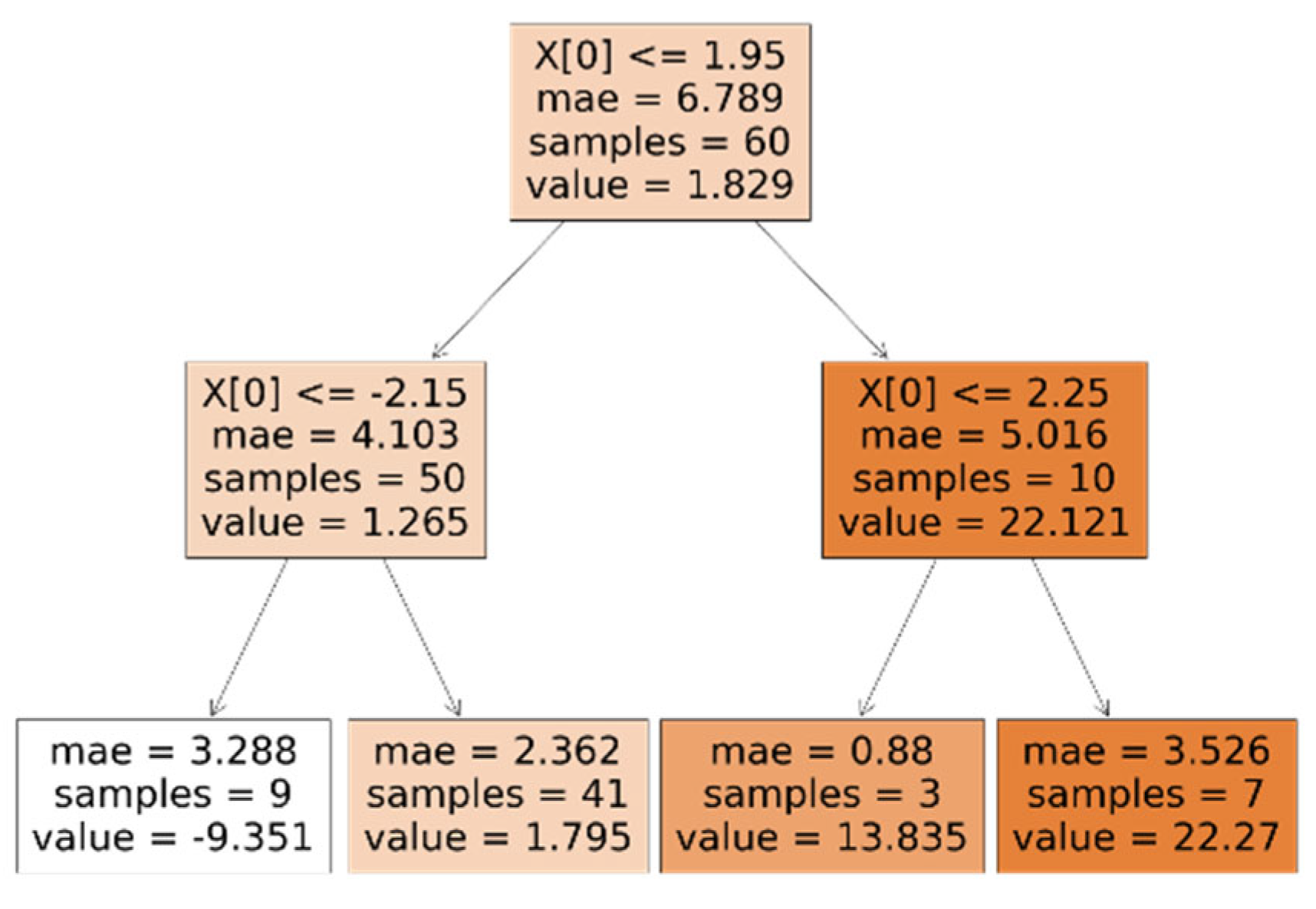
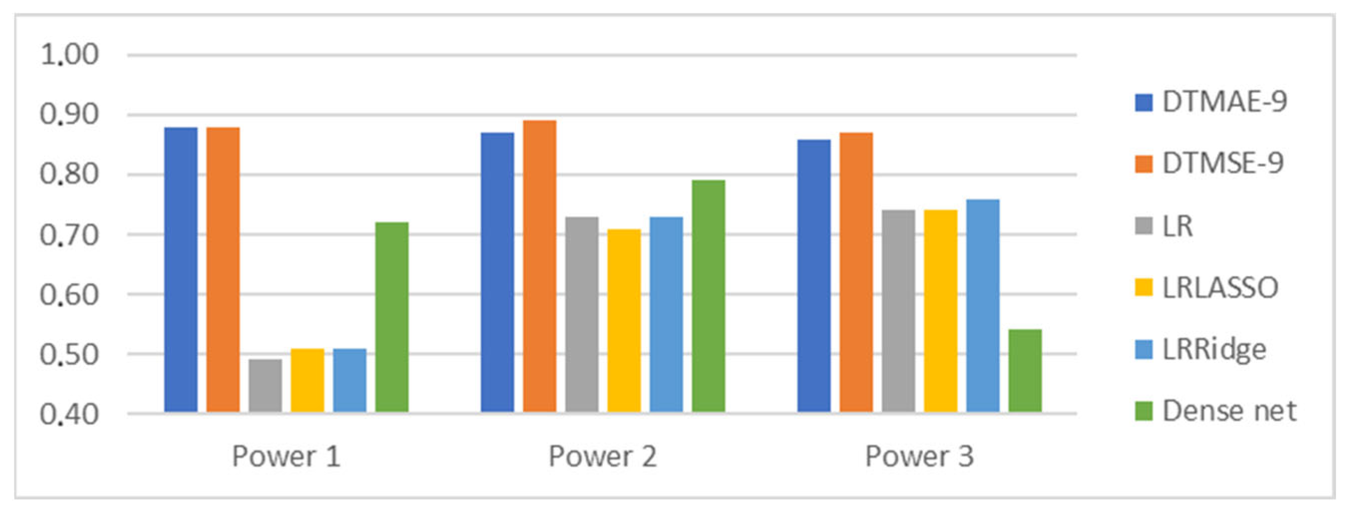
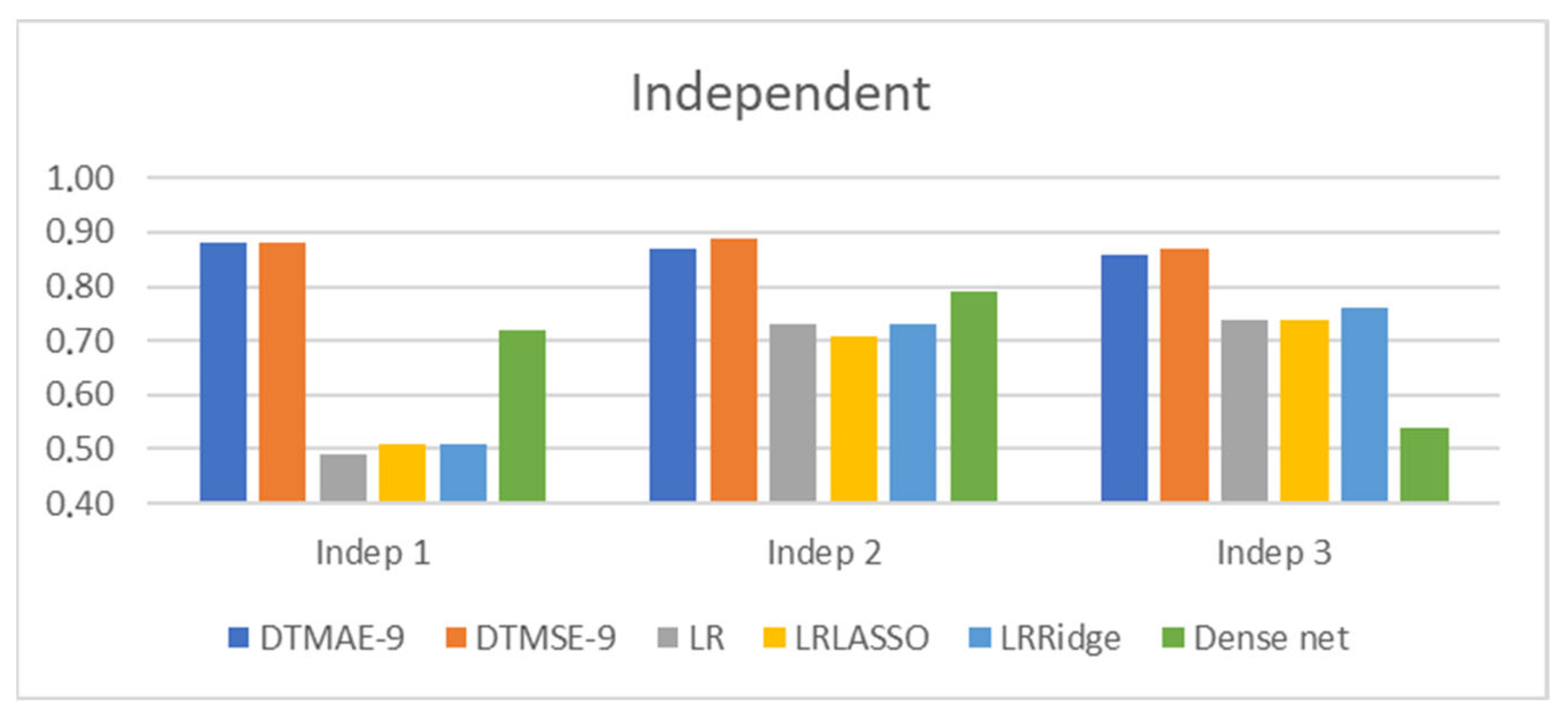
The effect of building configuration on the annual thermal and lighting energy demand and human comfort performance derived from energy demand results can be proven indirectly. In the framework of applying building regression models (decision tree, linear regression, and dense neural network) with the purpose of estimating annual heating energy demand, the first test was carried out without using any configuration descriptors. In this case, the highest model accuracy was only R² = 0.74. By extending the input variables with a configuration identifier, which identifies the configuration but does not contain any information about its geometry, the accuracy increased to R² = 0.8. The estimation accuracy of the regression models using the configuration identifiers is shown in Figure 11.

When the accuracy doesn’t change with further increasing input and model complexity, the maximum accuracy is reached. The performance of linear regression-based models (LR, LRLASSO, and LRRidge) could be improved using input variables on the second and third powers. Decision trees and dense neural network-based models are able to estimate non-linear functions themselves; they do not require additional non-linearity in the inputs. Therefore, the performance of decision trees (DTMAE-9 and DTMSE-9) decreases with further increasing input power. The model complexity of the dense neural network (Dense net) was not sufficient using only the first power of input; therefore, its accuracy reached its maximum with the second power. Better network structure selection would require only the first power of input. Unfortunately, the accuracy is limited to no more than R² = 0.88 without building configuration descriptors.

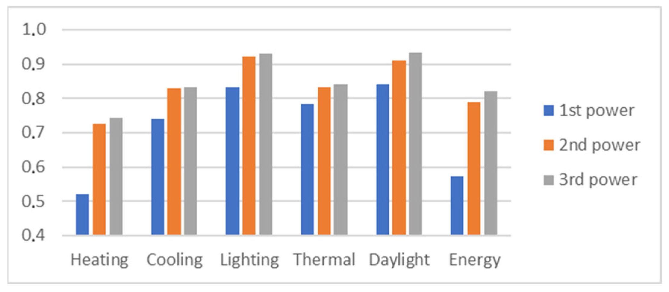
Figure 12 depicts the accuracy of linear regression estimations of all simulated result values (besides Heating: Cooling, Lighting, Thermal comfort, Daylight factor, and Total Energy). These characteristics show slight increases in accuracy estimates. This means that the main improvement is between the first and second powers of input variables, and above the third power, only slight increments are expected. Based on the depicted accuracies, increasing input complexity from the second to the third power does not have a significant gain. Therefore, further increments in input power are not reasonable. Furthermore, in other types of outputs excluding heating, the building configuration describing DV-s has less effect; however, the accuracy is still not at an acceptable range. The accuracy of estimations could only slightly exceed R² = 0.92 without building geometry descriptors; therefore, the indirect proof implies that considerably more accuracy can be achieved using building configuration descriptors.

7. Configuration Descriptors

As proven in the previous section, building configuration information should be applied among input design variables, and for this purpose, an appropriate representation is proposed. The quality of the representation means how well it is able to describe the important properties of the configuration and how much of the unimportant DV-s it contains. The applied method makes the plan digitalization process quick and easy, whereas instead of using predefined building plans, the model is created directly from 3d base space units in the form of cuboid building blocks, connected by their full sides. The set of examined models is reduced to 6-block buildings, which fit into a 5 × 5 × 3 space [24,25]. This reduction was based on architectural rules and regulations, which ensure that all applicable building configurations are examined, and the buildings are compliant residential houses. The building configurations, which are created using six building blocks, are then equipped with predefined wall structures and windows applying wall-window-rates, and finally, the buildings are rotated with their main façade to predefined orientations. Note that hereinafter, independent inputs refer to the situation where the above-mentioned building configuration information is not used, i.e., the necessity of the building configuration information is indirectly approached and visualized.

The proposed building plan discretization method makes the planning and generation of building designs simpler; however, this is not a concrete representation. The quality of representations strongly influences the regression model complexity and the approximation accuracy; therefore, different types of descriptors are examined. The creation of indirect descriptors requires involving architecture experts in configuration data pre-processing. Through this pre-processing, directly independent descriptors are expanded using analytical inspection of the simplified configuration structure. As a result, the following types of indirect descriptors are generated.

7.1. Single—But Complex Descriptor

When analyzing building shapes from the point of view of energy performance, transmission heat loss through the surfaces of building envelopes, as well as the heated internal volume or area, play the most critical role in climates with significant annual heating demand. Though the A/V ratio (the relationship between the external envelope surface and the heated indoor volume) [36] and the aspect ratio or shape factor (proportion of building layout length to width) [37] are one of the most commonly known expressions, buildings with the same shapes (A/V ratios) and volume rates can deviate in the number of stories as well as the layout solutions; hence, compactness is more appropriately described by the A/S ratio (envelope area divided by the heated floor space) of (17). This descriptor is proposed by Parasonsis et al. [38] in the form of “geometric efficiency (GE).” Such a descriptor is used in the following equation; however, in the applied formula, a specially selected coefficient is used that expresses the proportion of less heat loss through the slab towards the soil (the floor structure of the ground floor). This coefficient (0.71) was calculated as the average value of the simulated transmission loss results of multiple models.

$$\frac{A_{env}}{S_{tot}}=\frac{A_{env-air}+A_{env-ground}·0.71}{S_{tot}}$$

(17)

where A_env-air is the building envelope structure facing the environment’s ambient air, i.e., the surface of the roof and façade structures in m², A_env-ground represents the floor surface adjacent to the ground in m², and S_tot is the total net floor space in m².

7.2. Set of Simple Variables

As the second indirect configuration descriptor, a set of 14 simple values is used. The values are the result of counting the special surface elements of the building envelope, vertices, and edges listed in

Table 3. Set of simple building configuration descriptors.

Surfaces	Vertices	Edges
Ground	Ground positive	Ground
Roof	Arcade positive	Roof positive
Base	Arcade positive air	Roof negative
Wall		Arcade positive
Arcade		Arcade negative
		Arcade positive air vertex

.

The regression models use the engineering parameters of the simulation (orientation of the main façade, wall-window ratio, wall structure) without pre-processing, but the building configuration descriptors are pre-processed. Therefore, such regression models are called indirect regression models.

To exclude human intervention and utilize the advantages of machine learning, building configuration descriptors should be conducted directly without pre-processing. Regression models with inputs that don’t use pre-processing are called direct regression models. In the following chapters, direct building configuration descriptors are proposed.

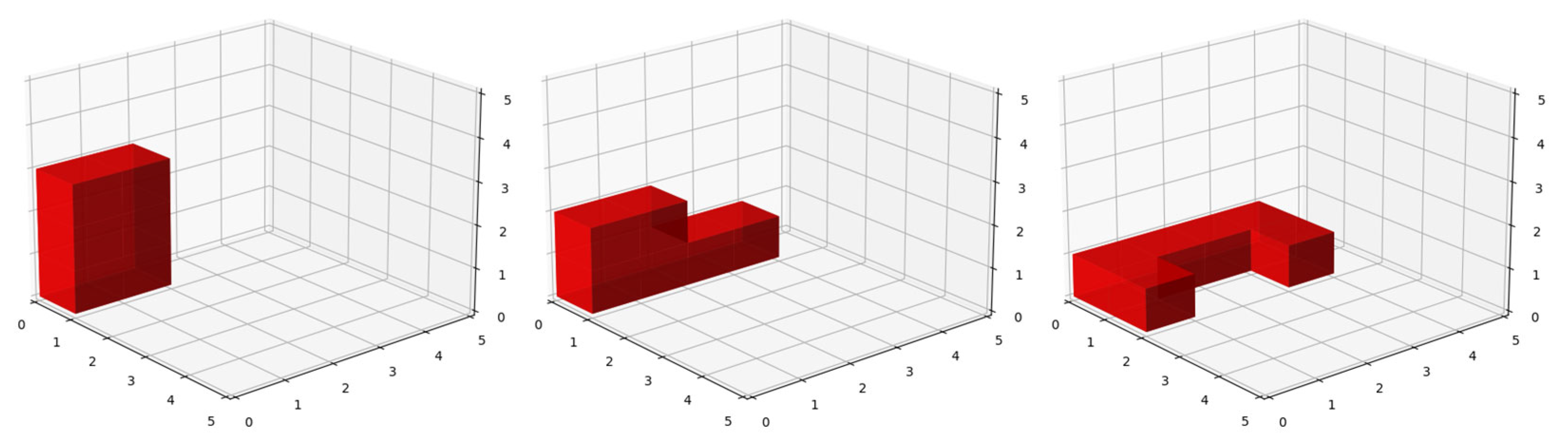
7.3. Coordinates

The first direct descriptor set contains the 3D coordinates of the building blocks, as presented in Figure 13. i.e., 18 coordinates are used as a configuration descriptor.

This set of descriptors is not dynamic because the number of building blocks is an indirect hyperparameter of the model. Therefore, it has an influence on the number of inputs and, through this, the model structure. Changing the structure of this input results in changes in the model; thus, a new regression model must be created.

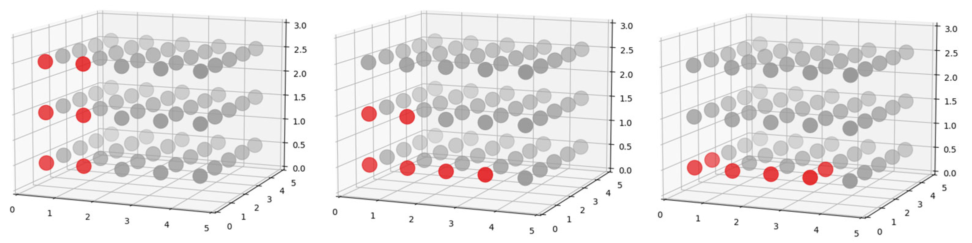
7.4. Point Cloud

In this representation, the full 5 × 5 × 3 search space is included in 75 building configuration descriptor inputs. As shown in Figure 14, the search space is discretized into equally sized blocks, which are the size of the building blocks. Each block of space is represented by its function. In the currently applied version, there are only two functions used: (grey-out of building and red-building).

An advantage of this representation is that changes in the number and function of building blocks do not require input, thus modelling structure change.

8. Results

The next section compares the R² score, mean squared error, and mean absolute percentage error with the standard deviation of the regression methods. Through the experiment, 10 measurements were made with all models and all input types. Figure 15, Figure 16 and Figure 17 contain averages of the accuracies measured by the R² score. Heating energy makes up the largest proportion of the energy demand, which is why this was prioritized for the regression model examinations. The 1, 2, and 3 indexes in the names of the models represent the maximum power of multiplicative combinations of input variables. The independent models do not use building configuration descriptors; only simulation parameters are used: wall-window-ratio, building orientation, and wall structure. Their accuracy is shown in Figure 15. Note that in the following figures, including Figure 15, numbers 1, 2, and 3 refer to the first, second, and third powers of the input. For example, Indep 1 (Indep 2, Indep 3) in Figure 15 represents the first power (second and third power) of building configuration-independent inputs.

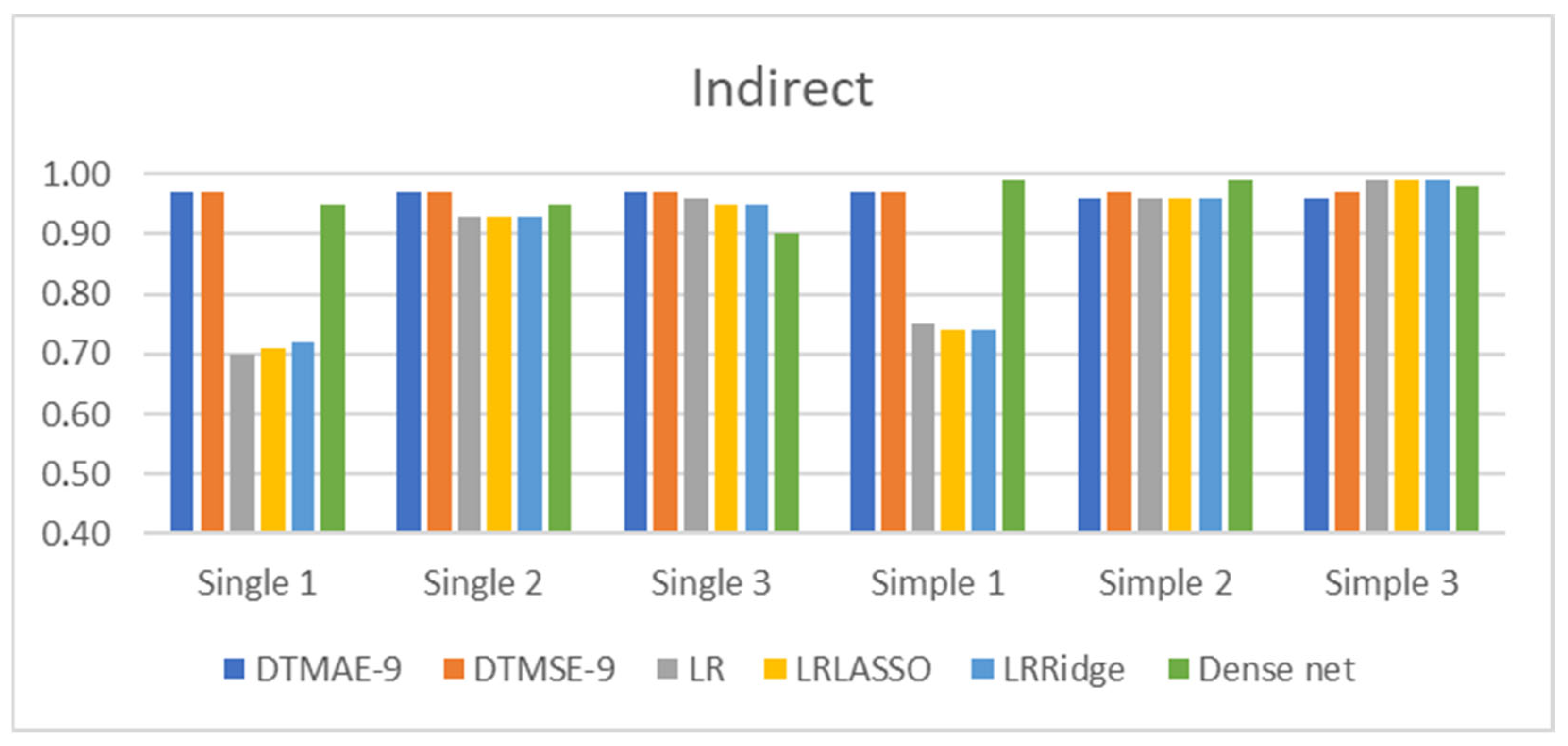
Indirect models, besides simulation parameters, use a single building configuration descriptor (A/S) or a set of descriptors made up of 14 simple values. Their accuracy is shown in Figure 16.

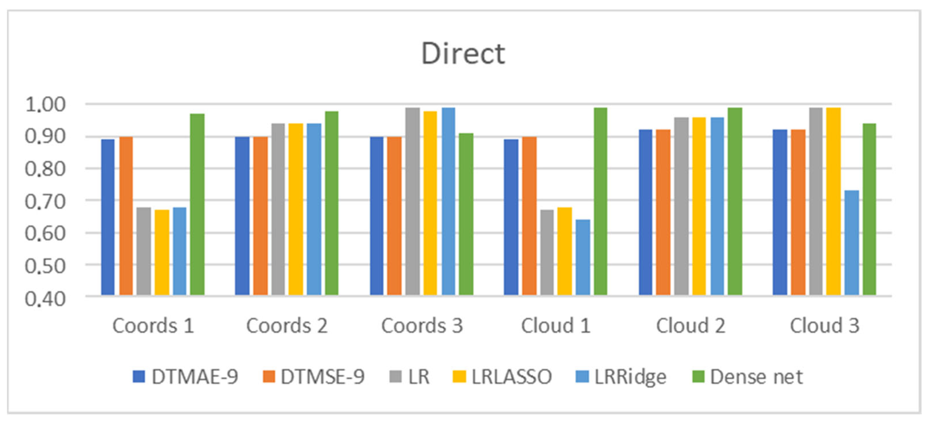
Direct regression, along with simulation parameters, uses configuration descriptors, from which the configuration can be restored. These are the 3D coordinates of the building blocks and the functional description of the search space, as represented by a point cloud. Their accuracy is shown in Figure 17.

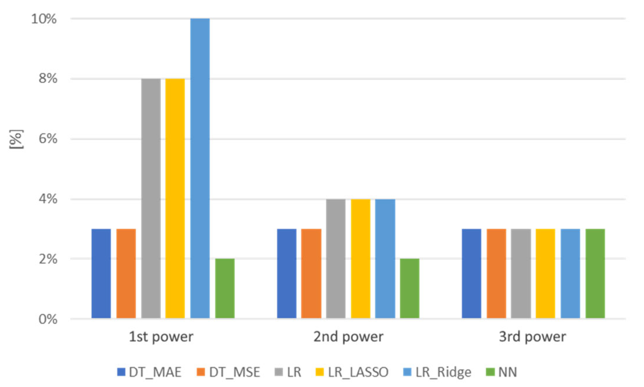
The R² score is adequate for comparing models and building configurations but is not descriptive enough for architects to make decisions due to the accuracy of the estimations and conclusions based on them. Figure 18 contains the standard deviation of 10 measures of the mean absolute percentage errors of all tested regression models.

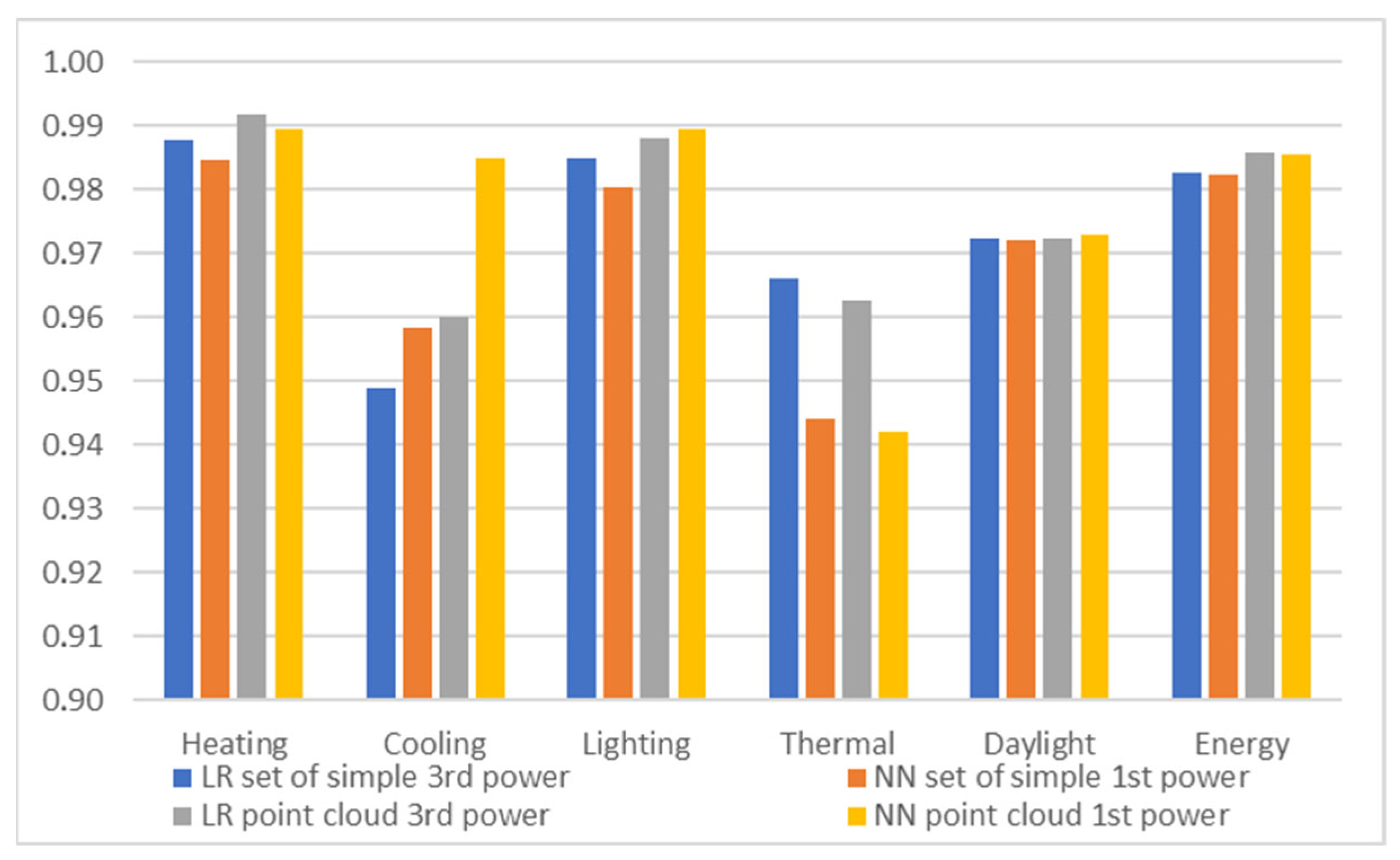
Based on the information depicted in Figure 15, Figure 16, Figure 17 and Figure 18 the following models were selected with both an indirect and a direct representation as the input. The first selected model is linear regression without regularization, and the second is a dense neural network. Both models use 14 variables in an indirect simple variable set and a direct, discrete functional point cloud representation. Linear regression uses the third power, while dense neural networks use the first power of these inputs.

Figure 19 shows the accuracy of estimation for all outputs made by selected models and inputs. It can be clearly seen that annual heating, lighting, and total energy demand can be precisely approximated by both regression models and both inputs with R² > 0.98.

The accuracy of daylight comfort is a bit lower but still above R² > 0.97 and the performances of the models are almost the same. The regression of annual cooling energy demand is R² < 0.96, except for the dense neural net with direct point cloud input, which performs very well, R² > 0.98.

That suggests that for annual cooling energy demand, the dense neural network can extract more descriptive features than indirect descriptors; therefore, linear regression with a higher power of input could be tested. In thermal comfort estimation, linear regressions performed much better than dense neural networks, which suggests that dense neural networks underfit the ground truth function; therefore, more complex networks could be tested.

9. Conclusions

It can be concluded that building comfort and energy estimations can be solved using regression models and that building geometry has a significant effect on energy performance. Based on examination and analysis of the results, linear regression using the third power and dense neural networks using the first power of inputs are proposed for building regression models to replace simulations for output comparison. In addition to simulation parameters (wall structure, wall-window rate, main façade orientation), an indirect set of simple configuration descriptors or point clouds of the search space is proposed as a building configuration descriptor input. Applying the proposed models and inputs, the least accuracy appears when estimating thermal comfort R² = 0.95, and the maximum accuracy R² = 0.99 is reached when estimating heating and lighting energy demand. The total energy demand estimation accuracy is over R² = 0.98, which is considered acceptable by architects. With reference to performance, reliability, and further development issues, a dense neural network with the first power of point cloud input is proposed for an adequate estimation of building energy demand and comfort data.

The presented method cannot be used as a generic model for accurate building energy demand estimation since the HVAC system was not considered a design parameter; however, it is applicable for comparing different building configurations. These regression models can not only simplify, i.e., substitute extensive simulation computation demand; however, they can also significantly contribute to future research in the development of automated building geometry generation using passive and active system combination decision processes for building comfort and energy optimization.