Article

Nexus between Energy Consumption, Foreign Direct Investment, Oil Prices, Economic Growth, and Carbon Emissions in Italy: Fresh Evidence from Autoregressive Distributed Lag and Wavelet Coherence Approach

1
Department of Management and Business Administration, “G. D’Annunzio” University of Chieti-Pescara, 65127 Pescara, Italy
2
Department of Economic Studies, “G. D’Annunzio” University of Chieti-Pescara, 65127 Pescara, Italy
3
International Institute of Islamic Economics, International Islamic University, Islamabad 44000, Pakistan
4
Department of Advanced Technologies in Medicine and Dentistry, “G. D’Annunzio” University of Chieti-Pescara, 66100 Chieti, Italy
*
Author to whom correspondence should be addressed.
Energies 2023, 16(16), 5885; https://doi.org/10.3390/en16165885
Submission received: 30 June 2023 / Revised: 31 July 2023 / Accepted: 5 August 2023 / Published: 9 August 2023
(This article belongs to the Section C: Energy Economics and Policy)

Abstract

:
The aim of this study is to explore the impact of economic growth (GDP), energy consumption, foreign direct investment, oil price, and exports on carbon emissions by employing yearly time series data for Italy for the period 1971–2019. For this purpose, we employed the autoregressive distributed lag (ARDL) model and wavelet coherence approach to analyze the interconnections among variables. The cointegration results confirm the long-run association between our variables. Our findings show that GDP has a positive impact on carbon emissions, while the square of GDP has a negative impact, thus confirming the presence of the EKC hypothesis. Further, oil prices have a detrimental impact on carbon emissions both in the long- and short-term; on the contrary, foreign direct investment, energy consumption, and exports promote environmental degradation. We propose some important policy recommendations based on these findings to address the environmental constraints.

1. Introduction

The world environment is highly disturbed due to the production and consumption activities of human beings around the globe. On a daily basis, print, electronic and social media update us with different kinds of natural disasters from different corners of the world; those disasters include fire, land sliding, windstorms, flooding, and insect and pest outbreaks. For example, the outburst of flooding in Australia and Pakistan, wildfire in Russia, Japan’s tsunami, and the earthquake in Haiti are all outcomes of climate change. Climate change is also responsible for the diminishing of glaciers, similarly, the early melting of the rivers and stream ice. Moreover, global warming and climate change have widely affected the health of small living organisms to the largest ones because, with the environmental change, the quality of drinking water is becoming poor each next day; as a result, the contaminated water is a source of multiple diseases such as diarrhea, hepatitis A, cholera, dysentery polio, and typhoid. Similarly, global warming and environmental change have polluted the air; air pollution is also a source of multiple diseases like chronic obstructive pulmonary disease (COPD), ischemic heart disease, lung cancer, stroke, and lower respiratory infections in children. Carbon emissions (CO2) represent a significant force in the degradation of overall environmental quality.
However, the production activities and the modification of land are rendering the emission of CO2 [1]. In awe of the increasing threat from global warming, developed and developing nations have ratified international agreements for the reduction of CO2 emissions, such as the Kyoto Protocol and the Paris Agreement [2]. The Paris Agreement was initiated in December 2015 with the main objective of combating global warming. It is concluded by the [3] that most of the developing countries, such as Turkey, South Africa, and India, are contributing to greenhouse gases (GHGs), especially CO2 emissions. Now, in modern-day environmental pollution is one of the major issues; therefore, the research on environmental quality and those influential factors involved in CO2 emissions [4,5,6,7,8].
Basically, environmental change is accelerated due to rapid industrialization, population growth, and increasing energy consumption. Meanwhile, CO2 emissions are the main source of the greenhouse effect. In the last three decades, the relationship between economic growth (GDP) and CO2 emissions has been extensively examined by a large number of researchers. Additionally, the emissions of greenhouse gases and their ultimate impact on climate change are at the forefront of policy debates. However, those countries that had signed the pact in the mid of 1990 realized that stronger rules and regulations were required to minimize the emission of CO2. Similarly, in 1997 the Kyoto Protocol’s aim was to legally bind the reduction in carbon, and the given target for the developed countries was enforced; in addition, the second era of the Kyoto Protocol was started on the 1 January 2013 and ended in 2020.
Hence, avoiding carbon emission in such an alarming situation is the need of hours because Mother Nature is completely disturbed by the ongoing production and consumption activities of human beings. One of the main forces which is playing a crucial role in the degradation of the environment is carbon emission. CO2 emissions are accelerated by energy consumption which is used as a factor of production. In the modern world, the race for higher growth among nations has further increased CO2 emissions. While taking the environment into consideration, the Environmental Kuznets Curve (EKC) hypothesis has become an obligatory argument in the literature of economics.
However, to identify the connection between economic growth and pollution [9], developed the well-known EKC hypothesis; according to the EKC hypothesis, in the early stages of economic growth, the environmental quality degrades, but if the income level of a country reaches that specified threshold the environmental quality starts improving. The main argument of the EKC hypothesis is that the countries with higher income are able to avoid environmental degradation because of the better systems with the adoption of green technologies; in contrast, the developing countries are not this able to cope with environmental problem degradation the way developed economies has taken over this issue due to insufficient resources [10]. Through the canonical work of [9], we can trace the EKC hypothesis, formally known as the EKC by Kuznets [11], who initially exposed the correlation between economic growth and income inequality which is U-shaped. For more than 20 years till that date, the relationship between economic growth and carbon emission has been a hotspot for a large number of researchers who have tested this relationship under the EKC hypothesis [12,13,14,15,16].
Therefore, the main concern in the case of economic growth, which is dependent upon energy consumption (EC), has become a source of discussion for environmental economists, especially in the 21st century. The EC plays an important role in the derivation of global warming [17]. As mentioned above, economic growth depends upon the EC; Ref. [7] has clearly mentioned that the magnificent development of economies around the globe has increased the demand for energy consumption, such as fossil fuel. In addition, the world energy outlook has identified that this demand will further grow by 48% for the period of 2017 to 2040.
By tradition, energy intensity in Italy is at the lowest level; at both levels of GDP and household consumption. The Italian National Agency of Energy Consumption (ENEA) reports that the primary EC in 2019 was 151.5 million tons of oil equivalent (Mtoe); however, since 2005, EC has declined with resemblance to the 1950s EC; the overall consumption of energy in 2019 stood at 111.2 Mtoe. Moreover, it is reported on a sectoral basis that the drop in the EC is due to the reduction in the EC share of the industrial sector (−35.3%), similarly, the transport sector (−10%), in contrast, the energy in the services sector was (+36.8%), accompanied by the households (+12.2%) in the period of 2000 to 2019. This meant that the Italian economy could not achieve a zero-carbon footprint in terms of energy use. However, it has been reported that, compared to other countries in the European Union, Italy’s government gives environmental issues less priority. The lack of a comprehensive strategy to reduce pollution is often mentioned as a major flaw in Italy’s environmental strategy. There is also no explicit carbon or environmental tax in Italy, and the country has no set goal for reducing its carbon footprint. Figure 1 shows that in 2018, after Germany, Italy was the EU member with the second-highest CO2 emissions. Therefore, Italian policymakers are curious about the variables that threaten Italy’s ability to maintain a healthy ecosystem. The targets which are set by the National Integrated Energy and Climate Plan (PNIEC) to be achieved by 2030 are renewable energy, reduction in CO2 emissions, energy efficiency, and energy security for development and sustainable economic growth.
Further, not only the developing but the developed countries also rely on the inflow of foreign direct investment (FDI) in the country. Though, the inflow of FDI is helpful in the creation of employment opportunities, the enhancement of productivity, the diffusion of technology, the formation of human capital, and economic integration [18]. On the one hand, economists have stated that FDI is a source of sustainable economic growth, and it also introduces innovative technologies in the host country [19]. On the other hand, policymakers and researchers have also indicated that the inflow of FDI is degrading the quality of the environment [7,20]. Moreover, it is also claimed that the FDI through polluting industries is causing CO2 emissions. This way, FDI is degrading the environment of the host country [21,22].
Based on the above discussions, the present work aims to empirically evaluate the relationships between GDP, oil price, foreign direct investment, energy consumption, exports, and CO2 emissions in the presence of the EKC hypothesis by utilizing annual data for the period 1971–2019. To this purpose, this study contributes to the existing literature in numerous ways. First, to our best knowledge, no study has yet explored the relationship between CO2 emissions, GDP, oil price, foreign direct investment, energy consumption, and exports in the context of the EKC hypothesis, particularly in the case of Italy. Second, most of the researchers in the literature examined the relationships among the above variables by utilizing traditional econometric approaches such as DOLS, FMOLS, and VECM. However, the current study applies the ARDL approach with OLS and FMOLS models as robustness to examine the variable’s long- and short-run dynamics. Further, this study also employs the wavelet coherence approach to obtain information on the association between carbon emissions and other variables at various frequencies and time periods. The main benefit of the wavelet technique is represented by its capacity to demonstrate the mechanics of evolving trends, cyclic arrays, and non-stationarity issues, which is crucial for understanding economic factors. The wavelet coherence (WTC) and the continuous wavelet transform (CWT), which are elements of the wavelet analysis, provide a deeper understanding of the interactions among variables at various frequencies, in-phase and out-of-phase co-movements, and lead/lag variables. The wavelet technique also enables more precise monitoring of shocks that alter the course of the business cycle. To our best knowledge, no previous studies have used this technique to gather information on the relationships and causality between the above variables in Italy at various frequencies and time periods.
The rest of the study is organized as follows. The pertinent literature is reviewed in Section 2. Information about data, variables, models, and estimation methods is provided in Section 3. The empirical findings are discussed in Section 4. Finally, Section 5 summarizes general findings and their implications for policy and practice.

2. Literature

2.1. GDP and CO2 Emissions

By using different econometric approaches and datasets, various studies examined the validity of the EKC hypothesis for individual and group countries. The empirical studies that examined the relationship between economic growth and CO2 emissions in the form of the Environmental Kuznets Curve Hypothesis (EKC) included [22] Pakistan, [23] ASEAN countries, [24] China and India, [25] Turkey, [26] and the USA. However, the literature provides diverse findings about the existence of the EKC hypothesis. For example, some researchers support the existence of the EKC hypothesis, whereas some studies revealed a U-shaped connection between GDP and environmental degradation and confirmed the non-validity of the EKC hypothesis. Ref. [27] conducted research on the linkage between GDP and the environment in Singapore and confirmed the validity of the EKC hypothesis. Similarly, Ref. [28] examined the linkage between GDP and environmental degradation and suggested the EKC hypothesis. Ref. [29] observed the connection between GDP and CO2 emissions in six West African nations. They employed a panel quantile approach for empirical analysis. Their findings confirmed the non-validity of EKC.
Ref. [30] studied the correlation between CO2 emissions and GDP in Vietnam. They examined this relationship by applying cointegration and causality techniques. The results of the study showed a long-term connection among research factors. Further, [31] also confirmed the presence of EKC by using annual time-series data of GDP and CO2. The results of the ARDL approach showed that the relationship between economic growth and CO2 emissions is positive, while the relationship between the square terms of economic growth and CO2 emissions is negative. These outcomes confirmed the validity of the EKC hypothesis in the BRIC.
Further, Ref. [32] explored the linkage between CO2 emissions, EC, and GDP. Their long-run outcomes established the presence of the EKC hypothesis. In the case of China, Ref. [33] examined the relationship between CO2 emissions, GDP, and EC by using data from 28 Chinese provinces. Their outcomes verified the non-validity of EKC. Ref. [22] researched the symmetric and asymmetric impact of GDP on CO2 emissions in Pakistan for the period 1971–2014. They applied the linear and nonlinear ARDL cointegration methodologies to confirm the EKC. The outcomes of both models established the validity of the EKC hypothesis. Ref. [34] investigated the relationship between CO2 emissions and their determinants in Turkey from 1960 to 2013. They found support in favor of the EKC hypothesis. Similar to this, Ref. [35] confirmed the EKC hypothesis in the BRICS nations. Ref. [36] studied the association between environmental degradation and selected indicators in Nigeria. Their outcomes suggested the presence of the EKC hypothesis. Further, Ref. [37] explored the connection between GDP and environmental deterioration in South Korea from 1971 to 2017. Their outcomes also confirmed the validity of the EKC hypothesis. In a similar way, Refs. [38,39] confirmed the validity of the EKC hypothesis in Indonesia and India, respectively. Table 1 lists existing studies that investigated the EKC.

2.2. Energy Consumption and CO2 Emissions

Using the ARDL and VECM Granger causality tests, Ref. [47] studied the relationship between CO2 emissions and non-renewable energy in China. According to their results, rising energy demand results in rising environmental degradation. Ref. [48] examined the nexus between EC and CO2 emissions in 25 OECD economies between 1990 and 2014. Their findings revealed that EC raises CO2 emissions. Similar findings were also reported by [49] for Indonesia and [50] for Pakistan. Ref. [51] analyzed the relationship between energy utilization and CO2 emissions in the USA. They discovered a statistically significant positive connection between energy utilization and environmental degradation. Ref. [52] explored the nexus among FDI, EC, GDP, and environmental quality in Turkey for the period 1970–2020. The outcomes of the novel dynamic simulated ARDL approach indicated that rising EC deteriorated the quality of the environment. Bangladesh [53] investigated the relationships between CO2 emissions and EC. By applying ARDL and the causality test, they confirmed linear causality between EC and CO2 emissions. Similar findings were also discovered by [54] in the case of Saudi Arabia. Ref. [55] investigated the influence of EC, GDP on environmental deterioration in Mexico and discovered a significant favorable influence of EC on environmental degradation. Similarly, Ref. [56] observed the interlinkages among GDP, EC, and CO2 emissions. Their findings revealed a positive association between EC and environmental degradation.

2.3. Foreign Direct Investment and CO2 Emissions

FDI and trade openness have frequently been studied in the literature when analyzing the influence of external elements on environmental sustainability in a country or region [57]. In this respect, Ref. [28] found that rising environmental contamination is a byproduct. Ref. [58] investigated the presence of PHH (pollution haven hypothesis) in 20 countries. They discovered that FDI increases pollution in emerging countries while lowering environmental degradation in developed countries. Furthermore, Ref. [59] looked at the connection between CO2 emissions and FDI in BRI nations. Their findings revealed the existence of PHH. Similar findings were made by [60], who discovered that FDI significantly enhances China’s environmental degradation. On the contrary, Ref. [61] revealed an insignificant linkage between FDI and CO2 emissions in BRI countries. Ref. [62] examined the influence of FDI, EC, tourism, and CO2 emissions in Bangladesh. The empirical findings illustrate a favorable effect of FDI on CO2 emissions.
Moreover, Ref. [63] utilized the dynamic simulated ARDL model to observe the impact of FDI on environmental degradation, and they observed that FDI promotes environmental sustainability. Ref. [64] studied the linkage between FDI and environmental deterioration in Pakistan. The findings demonstrated that FDI enhances ecological deterioration. Similar to this, Ref. [22] observed the linkage between FDI and the environment in Pakistan and confirmed the validity of PHH, while [65] studied the connection between FDI and CO2 emissions in developing nations. Their findings showed that FDI significantly and positively harms the environment. Moreover, Ref. [66] scrutinized the relationship between FDI and environmental deterioration in OECD nations and found that FDI promotes CO2 emissions. Ref. [67] examined the asymmetric connection among FDI, oil prices, and CO2 emissions by utilizing data from Gulf Cooperative Council economies. They discovered that FDI harms the environment and confirmed the PHH. Ref. [68] analyzed the consequences of FDI and other factors on India’s environmental quality and showed a positive correlation between FDI and environmental quality. Ref. [69] looked into the impact of GDP and FDI on the quality of the environment in 15 Asian emerging nations. They argued that FDI contributed to environmental deterioration, supporting the presence of PHH. By applying the PMG-ARDL technique, Ref. [46] analyzed the nexus between FDI and the environment in GCC nations. They identified that FDI exerts a long-term positive impact on the environment.

2.4. Exports and CO2 Emissions

Regarding the connection between EXP and environmental degradation, Ref. [23] presented a theoretical justification, arguing that EXP influences CO2 emissions through three channels. First of all, a rise in EXP raises energy demand [70]. Secondly, increased EXP necessitates greater usage of natural reserves [71]. Last but not least, increasing exports makes it necessary for businesses to be more competitive on a global scale, which lowers production costs and levels of carbon emissions through the use of technologically modern equipment [72,73]. While evidence suggests that higher EXP increases EC in the economy and thus degrades environmental quality if the country’s energy portfolio contains a higher proportion of clean energy, an increase in EXP will improve environmental quality. Ref. [74] explored the relationship between EXP and CO2 emissions in BRICS countries between 2000 and 2013. By applying the OLS method and panel quantile regression approaches, they discovered that EXP intensifies CO2 emissions. Ref. [75] examined the consequences of GDP, EC, and EXP on the quality of the environment in newly industrialized (NIC) nations between 1979 and 2017. The empirical results showed that EXP has a harmful impact on environmental sustainability. Ref. [76] studied the influence of FDI and trade on environmental quality in Turkey by applying linear and nonlinear ARDL techniques. Their outcomes demonstrated that negative shocks in EXP decrease environmental deterioration, while positive shocks in exports have no significant impact on environmental deterioration. Ref. [23] examined the impact of imports and exports on environmental quality in seven ASEAN countries, and empirical findings revealed a negative relationship between variables. Similarly, Ref. [77] scrutinized the link between EXP and the environment in Turkey and found that EXP exacerbates the country’s environmental problems. Ref. [78] also highlighted that export growth increased carbon emissions in 189 countries between 1990 and 2011. Ref. [79] also discovered a deteriorating effect of EXP on the quality of environmental data in 11 highly polluted Asian nations. However, with regard to a panel of 65 advanced and developing nations between 1981 and 2012, Ref. [72] discovered that higher exports are related to less environmental degradation.

2.5. Oil Price and CO2 Emissions

Another area of literature that has received significant attention in recent times is the connection between OP and the environment. The cost of energy plays an essential role in the growth of any economy. Oil price fluctuations have different impacts on oil exporting and importing economies. Numerous studies have documented that rising OP results in lower oil consumption, which in turn lowers environmental degradation [80,81]. On the contrary, a rise in energy costs signals a shortage of oil, which prompts the oil-importing nations that rely on that source of energy to look for alternative energy sources, hence lowering CO2 emissions [82]. Concerns about climate change and restrictions on oil imports from a selected group of suppliers (OPEC) are two additional elements that push oil-importing nations to expand their energy sources by switching to cleaner sources of energy [83,84,85].
Although empirical findings on the association between crude OP and CO2 emissions provide diverse outcomes, Ref. [86] explored the relationship between OP and environmental deterioration and suggested an inverse relationship, meaning that a rise in OP reduces CO2 emissions in Turkey. Ref. [87] observed that a rise in OP has a short-term effect on GDP and carbon emissions but a gradual long-run effect. Ref. [81] discovered an adverse impact of OP on CO2 emissions. Further, Ref. [22] assessed the impact of OP shocks on environmental degradation in Pakistan during the period 1971–2014. Their findings showed that increases in OP intensified environmental deterioration in the short run. Recently, Ref. [88] applied the FMOLS approach to explore the relationship among OP, EC, and CO2 emissions in 30 European countries and discovered a negative correlation between OP and CO2 emissions. In a similar way, Ref. [89] looked into the connection between CO2 emissions and OP in India and discovered a negative connection. Ref. [90] examined the effect of OP and oil price volatility on GHG emissions in 26 European Union countries, 22 oil-producing countries, China, and the USA using the Driscoll–Kraay model. The impact of oil prices on GHG emissions is asymmetrical between oil-exporting and -importing economies. Oil price increase in oil-importing countries reduces GHG emissions; contrarily, its impact enhances emissions in oil-exporting nations. Ref. [91] also revealed similar results in the case of G-7 countries. Their findings showed that OP and oil rents exert a negative impact on CO2 emissions and represent the major drivers of clean energy consumption. Ref. [92] examined the causal relationship between OP and carbon intensity in 28 European countries. The findings revealed an inverted U-shaped relationship between OP and CO2 emissions.
It is evident from this literature review that there has been much debate on the relationship between GDP, FDI, OP, EC, EXP, and CO2 emissions. However, to our best knowledge, we found no empirical study in the context of Italy. The originality of the present study is that it is the first study to use a wavelet coherence approach to gather information on relations and causal interactions among the above variables at multiple frequencies and timescales. As a result, the current study fills identified gaps in the literature in order to expand recent research on Italy and enlighten policymakers on environmental policies that will aid in the reduction of environmental pollution.

3. Data and Methodology

3.1. Data and Variables

The objective of the present work is to examine the causal connection among CO2 emissions, GDP, FDI, OP, EC, and EXP in Italy and to confirm the existence of the EKC hypothesis. To carry out the empirical analysis, we used annual data for Italy from 1970 to 2019. Carbon emissions (measured in metric tons) per person is our dependent variable, while the explanatory variables are gross domestic product (GDP) per person in constant 2010 US dollars, foreign direct investment (FDI) per person, oil prices (measured in dollars per barrel), energy consumption (measured in million tons of oil equivalent) per person and exports (constant 2010 US$) per person. Data for CO2 emissions, GDP, FDI, and EXP are collected from the World Bank database. Data regarding oil price and energy consumption have been taken from UNCTID and British Petroleum Statistical Review, respectively. Table 2 depicts the variables unit of measurement and sources. Further, in order to eliminate the heteroscedasticity issue, we transformed the variables by taking their natural logarithm. The econometric model we used to analyze the relationship among variables is as follows:
l n C O 2 t = β 0 + β 1 l n G D P t + β 2 l n G D P t 2 + β 3 l n F D I t + β 4 l n O P t + β 5 l n E C t + β 6 l n E X P t + μ t
where L N C O 2 t denotes logarithm of per capita carbon emissions, L N G D P t denotes logarithm of per capita GDP, L N G D P t 2 denotes square of GDP, L N F D I t denotes logarithm of FDI, L N O P t denotes logarithm of oil prices, L N E C t denotes logarithm of energy consumption and L N E X P t denotes logarithm of exports; μ t is error term and t denotes time period. According to the EKC hypothesis, the relationship between GDP and CO2 emissions should take the form of an inverse U-shaped curve. In the case of Italy, the EKC hypothesis is demonstrated to be true if the estimated value of GDP is positive and the square of GDP is negative.

3.2. Autoregressive Distributed Lag Model (ARDL)

Several econometric techniques have been utilized in the current literature to analyze the long-run connections among variables. Examples include the Philip-Hansen test [93], the FMOLS methodology [94], and cointegration methods [95,96]. However, the present study applied the ARDL cointegration methodology recommended by Pesaran et al. Refs. [97,98] to examine the long-term relationship between variables. This approach has a certain benefit over the other cointegration techniques. The primary advantage of the ARDL approach is that it does not require variables to have the same integration order. This approach can be applied as long as variables are I(0) and I(1) or a mixture of both. It estimates the short- and long-run dynamics in a single equation. It provides better outcomes even for small datasets than conventional cointegration techniques. We applied this technique to examine the long-term connection between CO2 emissions, GDP, FDI, OP, EC, and EXP. The UECM (unrestricted error correction model) for the ARDL approach is given as bellows:
Δ l n C O 2 t = β 0 + i = 1 p β 1 Δ l n C O 2 t 1 + i = 1 p β 2 Δ l n G D P t 1 + i = 1 p β 3 Δ l n G D P t 1 2 + i = 1 p β 4 Δ l n F D I t 1 + i = 1 p β 5 Δ l n O P t 1 + i = 1 p β 6 Δ l n E C t 1 + i = 1 p β 7 Δ l n E X P t 1 + λ 1 Δ l n C O 2 t 1 + λ 2 Δ l n G D P t 1 + λ 3 l n G D P t 1 2 + λ 4 l n F D I t 1 + λ 5 l n O P t 1 + λ 5 l n E C t 1 + λ 5 l n E X P t 1 + ε t
The optimal lag lengths can be determined by using the Akaike information criterion (AIC). The null hypothesis of no cointegration among variables ( H 0 :   λ 1 = λ 2 = λ 3 = λ 4 = λ 5 = λ 6 = λ 7 ) is tested against the alternate hypothesis of cointegration among variables ( H 1 :   λ 1   λ 2     λ 3     λ 4     λ 5     λ 6     λ 7 ) .
In order to determine the long-run cointegration among variables, the estimated value of the F-statistics is compared to the upper and lower critical boundary values. If the estimated F-statistics value is greater than the upper bounds of the critical values, the H0 of no cointegration can be rejected, meaning that a long-term cointegration exists among the research variables. On the other side, if obtained F-statistics value is smaller than the lower critical boundaries, we are unable to reject the H0 null of no cointegration, which suggests no long-term connection among research factors. However, the decision would be uncertain if the anticipated value of F-statistics falls inside the lower and upper critical boundaries, the decision would be uncertain.
After the validation of long-run relationship among variables, short-run dynamics are estimated by incorporating the error correction model (ECM) into the ARDL framework specified as follows:
Δ l n C O 2 t = β 0 + i = 1 p β 1 Δ l n C O 2 t 1 + i = 1 p β 2 Δ l n G D P t 1 + i = 1 p β 3 l n G D P t 1 2 + i = 1 p β 4 Δ l n F D I t 1 + i = 1 p β 5 Δ l n O P t 1 + β 6   Δ l n E C t 1 + β 7 Δ l n E X P t 1 + θ E C T t 1 + ε t 1
where θ is the associated coefficient of the ECT (error correction term), which also shows the speed of adjustment towards the long-run stability. The value of ECT should be negative and statistically significant.

3.3. Wavelet Coherence Approach

In addition, the present study also used the wavelet coherence approach to capture the correlation and causality between research factors simultaneously. We employed ADF and PP tests to study the integration order of GDP, FDI, EC, EXP, OP, and CO2 emissions. Additionally, structural breaks in variables were confirmed using the [99] stationarity test. In accordance with the objective of the study, we utilized the wavelet approach to learn more about the time-frequency dependency among GDP, FDI, EC, EXP, OP, and CO2 emissions in Italy, employing yearly data ranging from 1961 to 2018. Ref. [100] developed the wavelet approach. The time series variables are likely to exhibit non-stationarity at their level, which is a well-known and widely acknowledged fact. The underlying problem with frequency-domain approaches, notably Fourier Transformation, is that by relying solely on the frequency domain, the time domain information is essentially neglected [101]. Furthermore, the structural time series breaks have an impact on the expected outcomes of standard causality approaches with predetermined parameters (s). If the standard time-domain technique is not followed, time series variables that are estimated but not stationary will produce biased estimates [102]. Therefore, to avoid these complications in the estimations, the present study applied the wavelet coherence technique.
A wavelet ( ϖ ) belongs to the Morlet wavelet family presented in Equation (4) as follows:
ϖ t = π 1 4 e i ϖ t e 1 2 t 2
where ϖ represents the frequency employed to limited time series; i denotes p(t), \ = 0, 1, 2, 3, …, N − 1; and 1 .
Two basic factors of a wavelet are time and location (signified by k) and frequency (expressed by f). Time series is transformed to a time-frequency domain before being transferred to wavelet transformation, as stated by [103]. ϖ  is changed, leading to the development of k, f. This explanation is demonstrated by Equation (5):
ϖ k , f t = 1 h ϖ t k f ,   k ,   f R , f   0
Using the time series data p(t), Equation (6) displays the continuous wavelet function as follows:
ϖ p k ,   f = p ( t ) 1 f ϖ t k ¯ f d t
Refs. [55,104] assert that after adding coefficient ϖ in the equation, the time series variable p(t) is indicated to be revived in Equations (7) and (8). However, Equation (6) is used to estimate p(t) as follows:
p t = 1 C ϖ 0 w p ( a ,   b ) 2 d a d b b 2
To reflect the vulnerability of CO2 emissions, GDP, EC, FDI, OP, and oil price, the wavelet power spectrum (WPS) is demonstrated as follows:
W P S p ( k ,   f ) W p ( k ,   f ) 2
The cross-wavelet transformation (CWT) method converted the time-series variable in Equation (8) into Equation (9). In order to visualize any connection between two time series (p(t) and q(t)) in combined time-frequency-based causalities, we adopted the wavelet coherence technique. The (CWT) applied on the two-time series is given in Equation (9) below:
  W p q k ,   f = W p k ,   f   W q ( k ,   f ) ¯
The CWT of CO2 emissions, GDP, EC, FDI, OP, and EXP, in Italy using annual time series data covering the period 1971–2018 are shown by Wp(k, f) and Wq(k, f), respectively, as indicated by [105]. They also created the equation for squared wavelet coherence, demonstrated in Equation (10):
R 2 k ,   f = S f 1 W p q ( k ,   f ) 2 S f 1 W p ( k ,   f ) 2 S f 1 W q ( k ,   f ) 2
If the R2 (k, f) value is close to one, time series factors are related, or a causal relationship among variables exists at a particular frequency, which is enclosed by a black line and colored red. On the other hand, if it approaches zero, there is no indication of connection or causality between the two variables and is depicted by the blue color, although R2 (k, f) only conveys information about the degree of correlation between variables but not its direction. As a result, [105] established a method to identify wavelet coherence discrepancies by using deferral indicators in the wavering of two-time sequences [101]. The derived wavelet coherence difference mechanism equation is displayed in Equation (11) as follows:
ϕ p q k ,   f = t a n 1 L S f 1 W p j ( k ,   f ) O S f 1 W p j ( k ,   f )
where L stands for a hypothetical operator and O for a real part operator.

4. Empirical Results

4.1. Descriptive Statistics

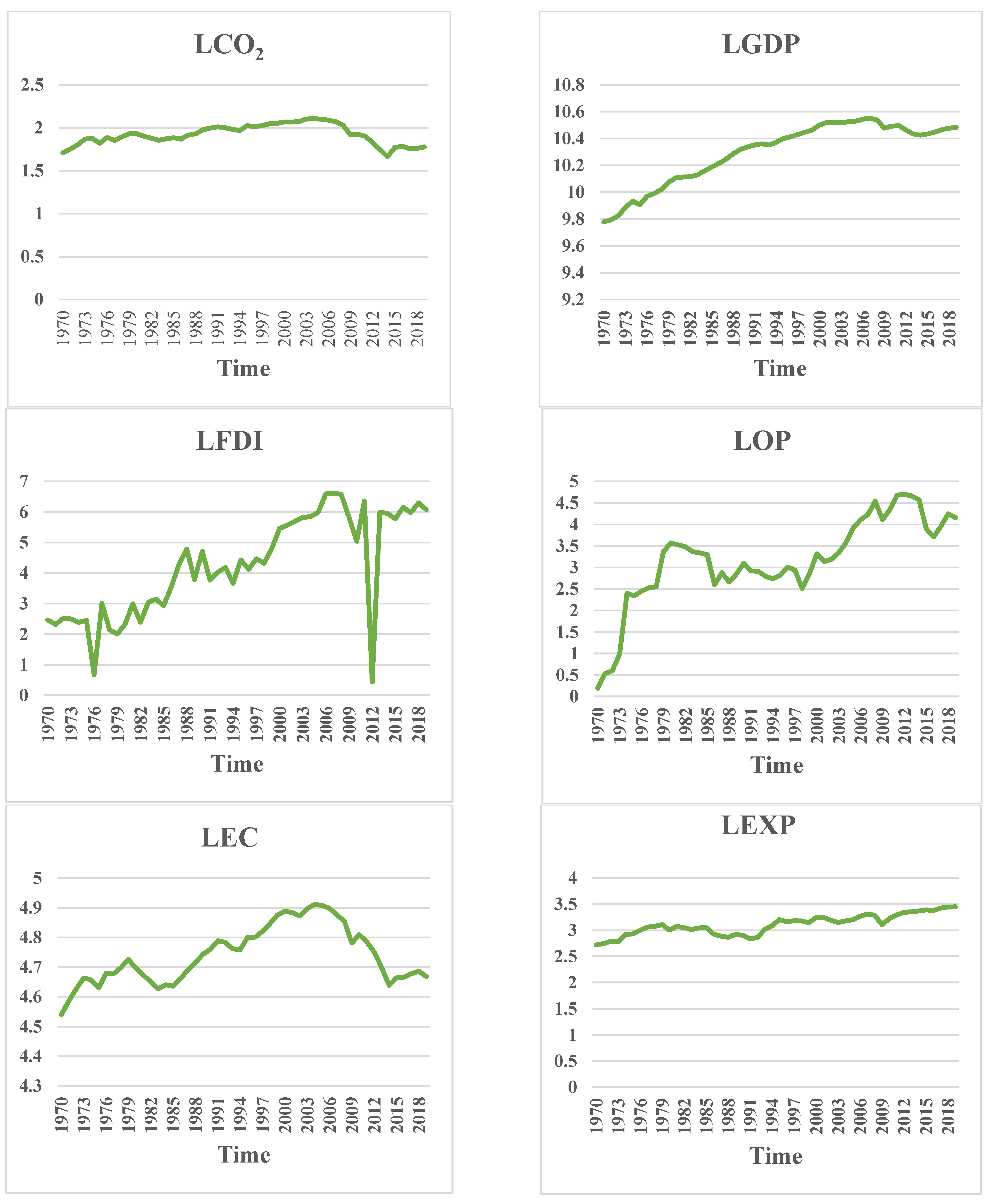
Table 3 presents the descriptive statistics of the considered variables. It is evident that GDP has the highest mean value, followed by EC, FDI, OP, EXP, and CO2 emissions. Further, the standard deviation is a measure that indicates how closely the data is grouped around the mean value. The closer the clustering around the mean, the lower the standard deviation. This reasoning leads to the conclusion that EC is closer to its mean, followed by CO2 emissions, EXP, GDP, OP, and FDI. The Jarque-Bera test reveals that each variable under consideration is normally distributed. Overall, the findings indicate that GDP, FDI, OP, EXP, EC, and CO2 emissions show a positive trend (Figure 2). Table 4 reports the correlation between the variables. The results illustrate that most variables are positively correlated with CO2 emissions, while exports are negatively correlated with CO2 emissions. Further, a significant and positive association is found between FDI, OP, EC, and EXP and GDP. Additionally, a moderately positive association was also discovered between EC and OP and EXP and EC. The significant correlation between the research variables demonstrates that any policy change for GDP, FDI, OP, EC, and EXP has a substantial influence on the environmental quality in Italy.

4.2. Unit Root Test Results

It is widely known that non-stationary variables might lead to spurious regression and biased analysis. It is important to analyze the stationarity properties of data series prior to evaluating the variable’s long- and short-run dynamics. We employed the two most popular stationarity tests, namely, the ADF and PP proposed by, respectively, to prevent the issue of spurious regression. Table 5 reports the results for both stationarity tests and illustrates that research variables contain a unit root since we cannot reject the null hypothesis of a unit root. But after taking the first difference, we can reject the null hypothesis of the unit root and confirms that all the variables become stationary. Since the traditional unit root test does not consider structural breaks in series, we also utilized the [99] stationarity test to capture the breaks in data series. The results of the structural break test are shown in Table 6 and suggest that variables at the level are non-stationary. However, after taking the first difference, the variables turn into stationary.

4.3. ARDL Results

The stationarity test results suggest that none of the considered variables is integrated at I(2). The next step of the estimation procedure determines whether there is a long-term link that exists among variables. For analyzing the long-term cointegration, we applied the bounds test cointegration approach. The null hypothesis of no cointegration among variables is tested against the alternative hypothesis of cointegration. Table 7 reports the outcomes of the bounds test cointegration approach and suggests that the estimated value of F-statistics exceeds the upper boundaries crucial values at a 1% significant level. This outcome explains that we can reject the null of no cointegration again the alternative and supports the hypothesis that CO2 emissions, GDP, FDI, OP, EC, and EXP have a long-term cointegration. The estimated outcomes of short- and long-term association among CO2 emissions and its influencing factors are reported in Table 8 and Table 9, respectively. The findings show that economic expansion has a favorable and statistically significant effect on CO2 emissions in Italy. According to this, a 1% upsurge in GDP led to a 14.89% long-term increase and a 35.52% short-term increase in CO2 emissions in Italy. In contrast, findings demonstrate that the squared of GDP has a detrimental effect on the level of CO2 emissions both in the long- and short-run. These findings show that for every 1% rise in squared GDP, CO2 emissions are reduced by 0.74% over the long term and by 1.71% over the short run. These results confirm the existence of the EKC hypothesis exists in Italy. These outcomes are consistent with the [41,42,45]. Turning to the OP, the results demonstrate that OP is adversely and significantly associated with CO2 emissions. According to these findings, a 1% rise in OP results in a considerable short and long-term decrease in environmental degradation by 0.027% and 0.04%, respectively. These results agree with those of [88,90]. Additionally, studies by [91,92] showed a negative correlation between OP and environmental deterioration and concluded that rising OP levels in G7 and EU 28 countries imply lower CO2 emissions. Furthermore, the results demonstrate that FDI has a negative effect on Italy’s environmental quality over the short- and long-term. According to the estimated results, a 1% increase in FDI considerably intensifies environmental degradation by 0.039% in the long term and 0.010% in the short run. These results confirm the existence of the pollution heaven hypothesis in Italy. Our findings concur with those [22] for Pakistan, [46] for the GCC countries, and [62,106] for Italy. In the case of EC, the estimated parameters of EC are positive and significant over the long- and short-term. These findings illustrate a 1% rise in EC enhances the environmental damage by 0.52% in the short-run and 0.60% in the long-run. This outcome is not surprising; many researchers have shown the negative effect of EC on environmental sustainability. Ref. [107] emphasized that EC is a major indicator of environmental deprivation and intensifies CO2 emissions. However, decreasing EC to lower CO2 emissions would not be an effective strategy for any industrialized country. The only way to improve the environmental quality without compromising the level of growth is by incorporating clean energy sources (e.g., biomass, solar energy, and wind power). These findings are in line with those of [108]. They investigated the cross-country and country-specific associations and discovered that the usage of clean energy is environmentally beneficial and enhances the quality of the environment, whereas the usage of traditional energy increases the volume of CO2 emissions, which worsens the environment. Finally, in the case of exports, the outcomes reveal that the exports are positively related to environmental degradation at a 1% significance level. These outcomes explain that a 1% increase in exports intensifies carbon emissions by 0.08% and 0.07% in the long- and short-run, respectively. Our findings are in line with other studies [74,77,79]. They stated a positive relationship between exports and environmental degradation. Furthermore, the coefficient value of the error correction term E C T t 1 is significant and negative. This finding also verifies the existence of long-term cointegration between variables and explains that any divergence from long-run equilibrium is fixed by 36.1% yearly.

4.4. Robustness Check

In this study, we also employed the DOLS and FMOLS methods to verify the robustness of ARDL estimates. Table 10 and Table 11 present the results of DOLS and FMOLS, respectively. These findings show that our ARDL results are in accordance with the DOLS and FMOLS estimates.

4.5. Diagnostics Tests Results

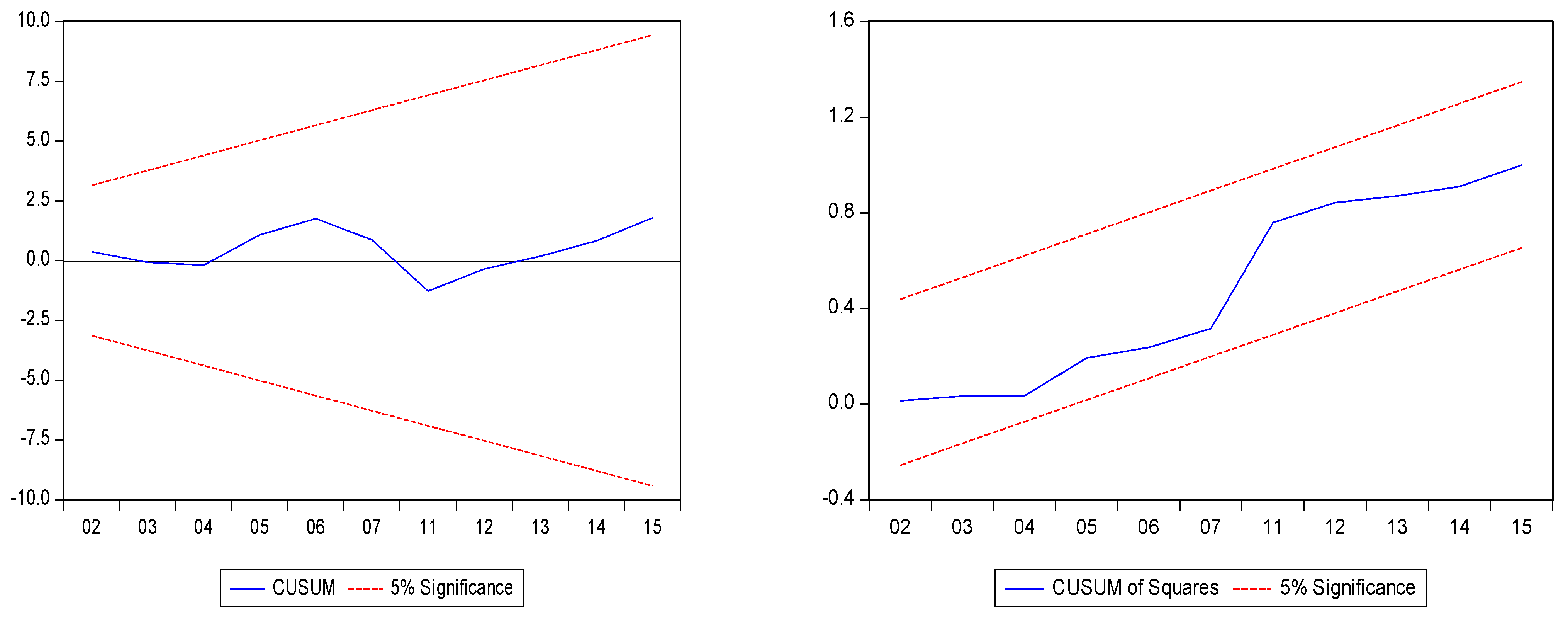
Additionally, we performed a number of diagnostic checks to make sure the model was stable. Table 12 presents the findings of serial correlation, normality, and heteroscedasticity tests. The outcomes of these diagnostics tests confirm that the underlying model is good and fits well. Further, to evaluate structural stability, we performed CUSUM and CUSUM-SQ tests. Figure 3 displays the CUSUM and CUSUM-SQ visual assessments, respectively. It can be established that model dimensions are reasonably stable if plots stay within a crucial boundary range of 5%. The graphs below demonstrate that CUSUM and CUSUM Square are inside critical boundaries.

4.6. Wavelet Coherence Approach

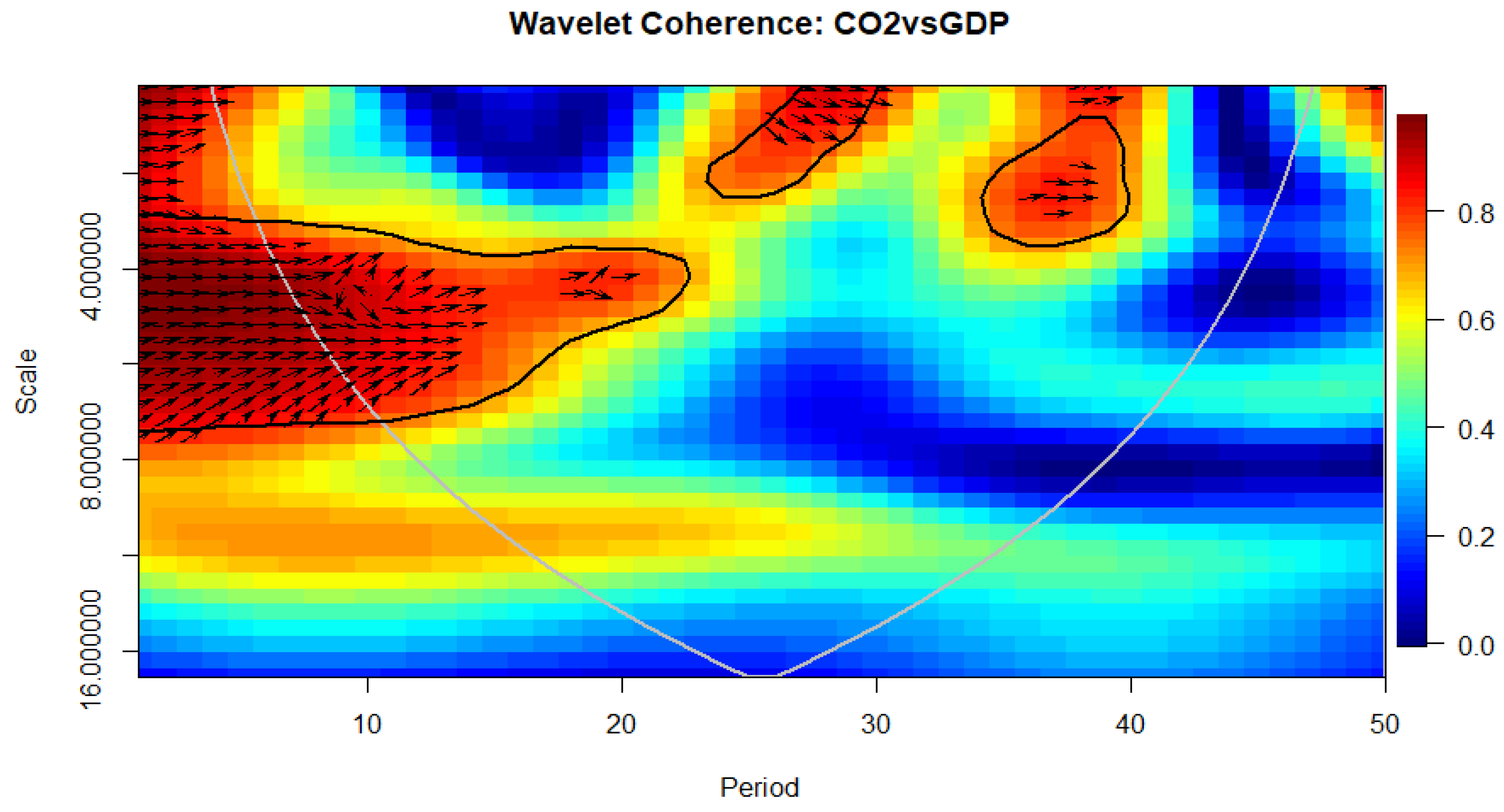
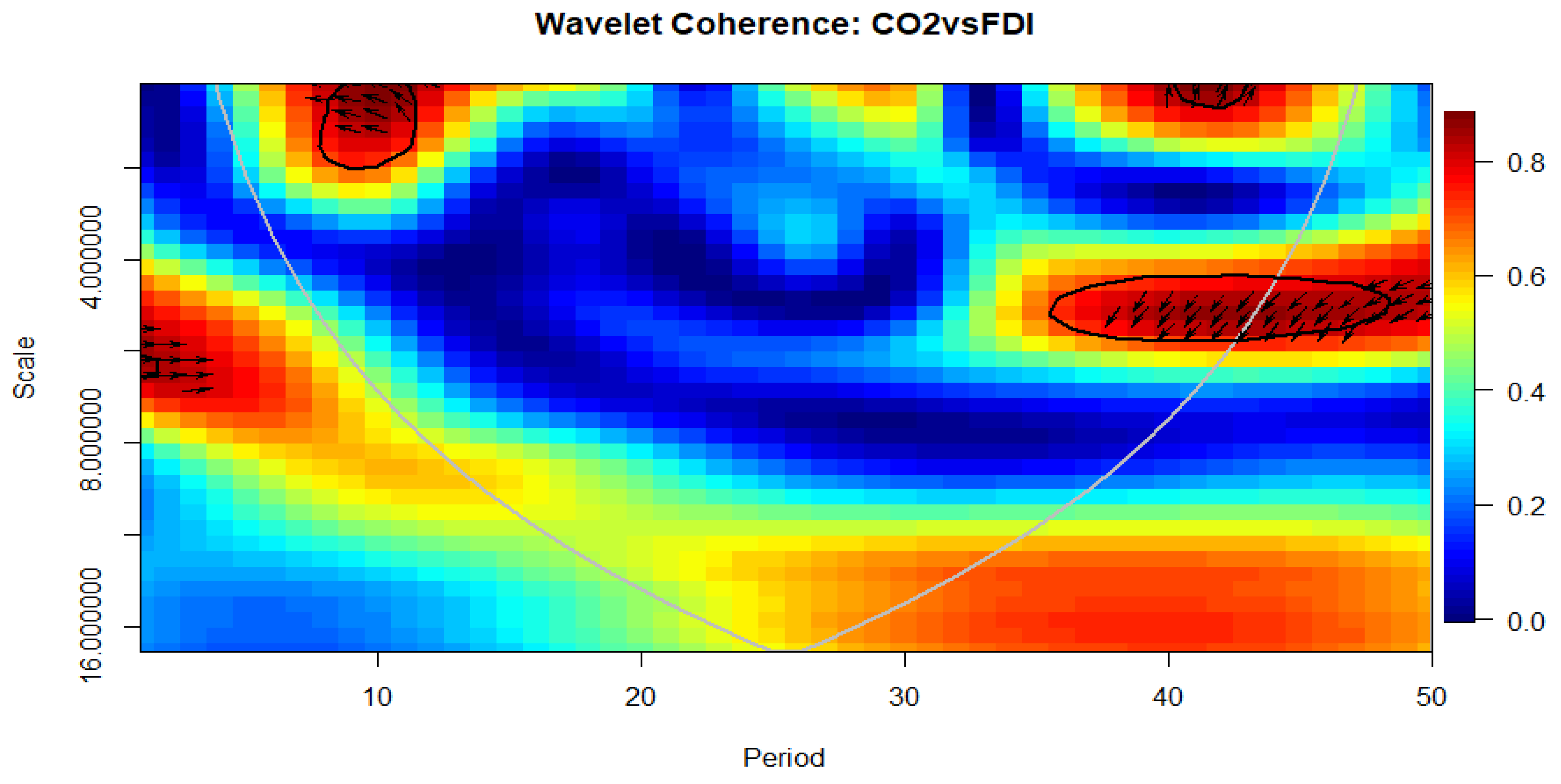
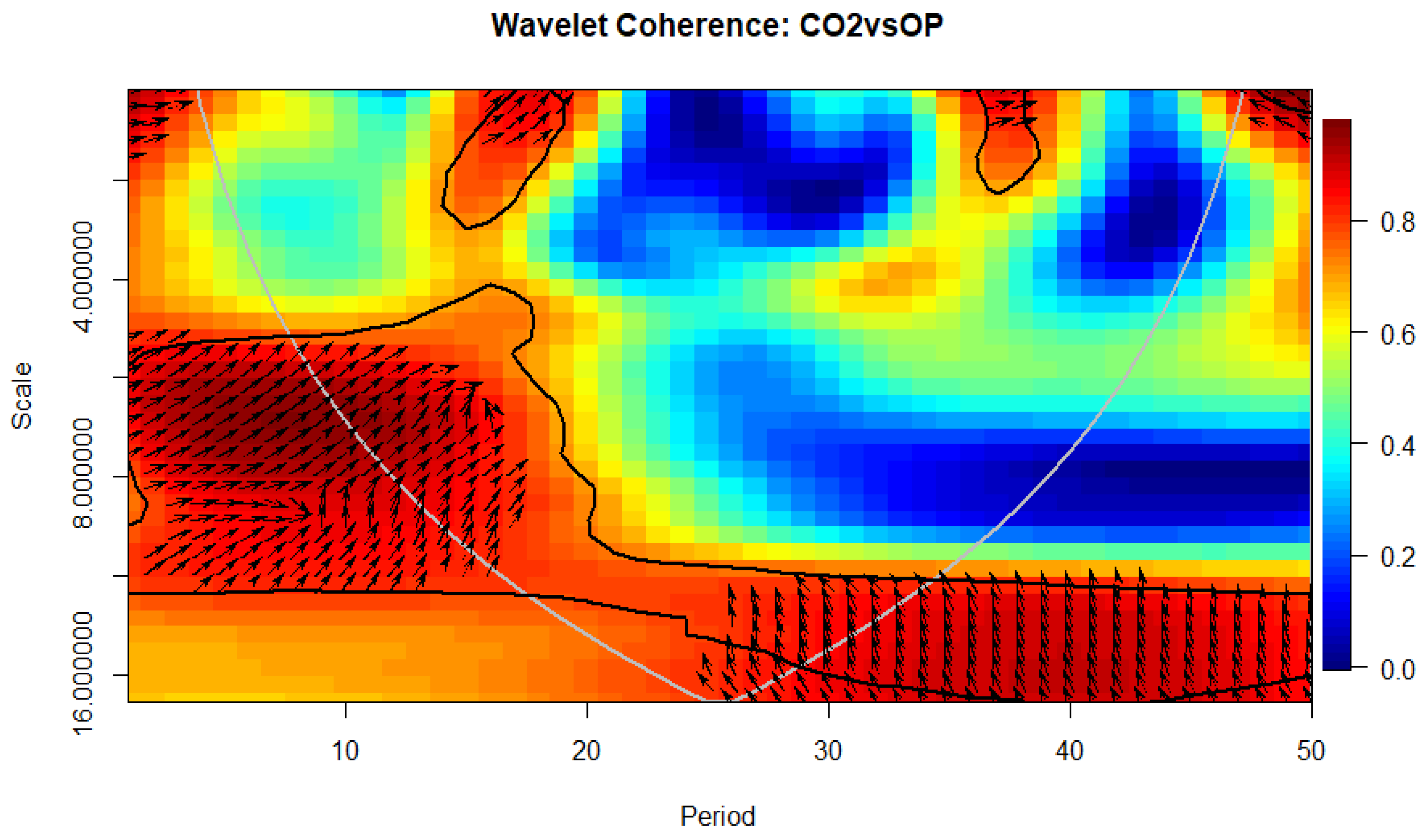
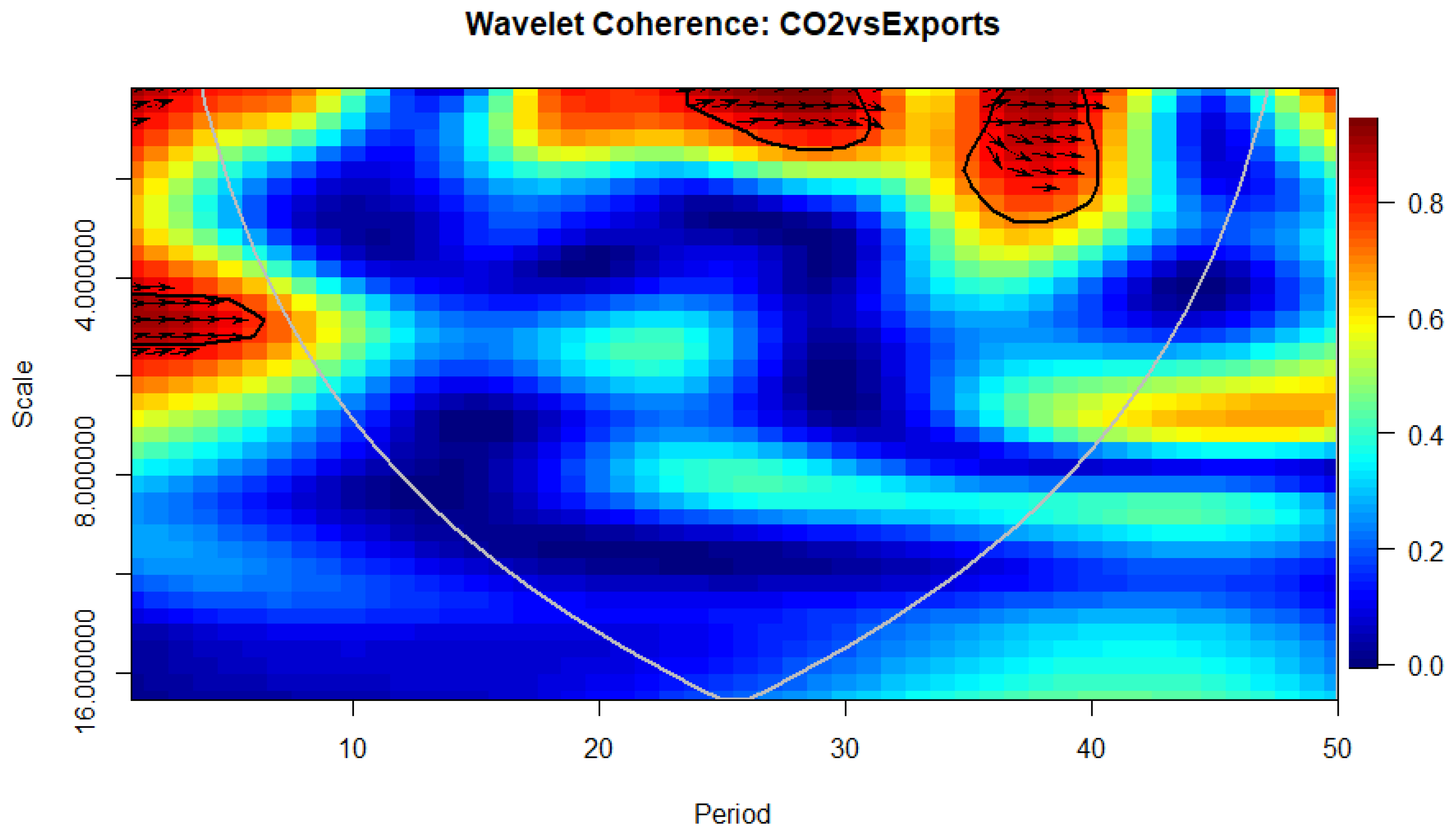
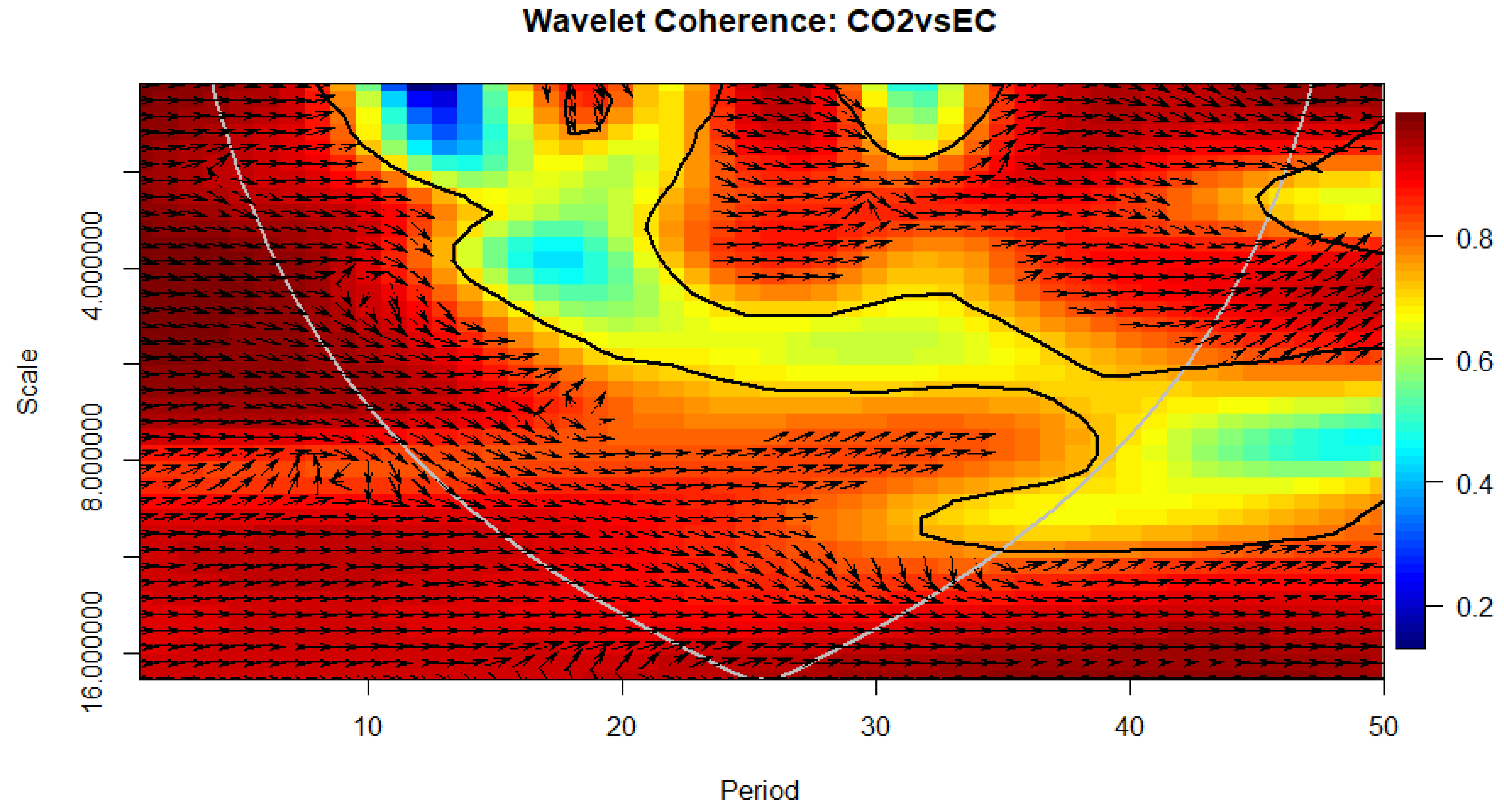
We also applied the wavelet coherence approach to capture the causation and correlation among CO2 emissions and regressors at various frequencies and time intervals. Wavelet coherence between Italy’s CO2 emissions, GDP, FDI, OP, EC, and EXP is depicted in Figure 4, Figure 5, Figure 6, Figure 7 and Figure 8. This technique was created in the field of econophysics to gather previously undiscovered evidence [104]. As a result, the current study investigates short, medium, and long-term causality and association among CO2 emissions and independent variables. The level of significance when evaluating wavelet coherence is indicated by a thick black contour centered on the Monte Carlo simulations. Moreover, periods 0–4, 4–8, and 8–16, respectively, show the short, medium, and long terms in Figure 3, Figure 4, Figure 5, Figure 6 and Figure 7. Furthermore, time is shown on the horizontal, and frequency is shown on the vertical axes, respectively [101,103]. The white line depicts the cone of impact or impact area that will be utilized for an explanation when studying wavelet coherence. The color range on the right side of the figure indicates how strong the correlation is. The cold blue color indicates lower reliance between the variables, whereas the red color denotes significant correlations between indicators. Further, cold places outside of significant areas show little reliance. Additionally, the thick black form in the figures, which was produced using a Monte Carlo simulation and exhibits significance at a 5% level. The direction of causality and correlation among research variables is portrayed by arrows in wavelet coherence. When two series have zero phase differences, they move in harmony on a specific scale. Positive and negative relationships among studied variables are depicted by the rightward and leftward arrows, respectively. When two variables are in phase, it means they are moving in the same direction; when they are out of phase, they are moving in opposing directions. Arrows indicating rightward down or leftward down suggest that the first series caused the second one, while arrows indicating rightward or leftward up show that the second series caused the first series. Figure 4 provides evidence of a positive link between CO2 emissions and economic development over the medium term at various scales (frequencies) between 1974 and 2010. Additionally, the upward and rightward arrows show that economic expansion in Italy drives CO2 emissions. Additionally, Figure 5 illustrates that between 1980 and 2010, at various scales (different frequencies), the medium-term arrows faced the left, indicating a negative connection between CO2 emissions and FDI. Additionally, the leftward falling arrows between 2005 and 2010 show that FDI is caused by CO2 emissions.
In Figure 6, between 1978 and 1988, at various scales (frequencies), rightward arrows show a positive and significant correlation between CO2 emissions and OP in the short and medium term. In addition, between 1995 and 2005 (long term), the leftward arrows show a negative correlation between CO2 emissions and OP. Also, a leftward upward arrow during this era indicates that OP causes CO2 emissions in Italy. In Figure 7, no evidence of correlation is found between CO2 emissions and EXP between 1974 and 1993 at different scales and different frequencies. However, between 1994 and 2010, rightward arrows depict a positive and significant association between CO2 emissions and EXP. Additionally, Figure 8 shows evidence of rightward arrows that demonstrate a significant and positive association between CO2 emissions and EC at various scales (frequencies) between 1974 and 2016. The rightward ascending arrows in the same era demonstrate that EC precedes CO2 emissions. In addition, a one-way causality runs from EC to CO2 emissions. This conclusion implies that EC is a key predictor of environmental degradation in Italy.

5. Conclusions and Policy Recommendations

The present research aims to examine the relationships between GDP, FDI, OP, EC, and CO2 emissions by using annual time data for Italy from 1970 to 2019 in the presence of the EKC hypothesis. The long- and short-run relationships are evaluated by using ARDL developed by [97,98] DOLS and FMOLS approaches. We also used the wavelet coherence approach by [100] to examine the correlation between CO2 emissions, GDP, FDI, OP, EC, and EXP. The uniqueness of this technique is that it ascertains short- and long-run connections and causality among variables simultaneously at various time intervals and frequencies. The results of the stationarity tests confirm that none of the variables under investigation are integrated at I(2). Further, the bounds test cointegration results provide evidence that variables have a long-term cointegration. The ARDL results suggest that GDP has a positive impact on environmental degradation, while the square of GDP has a negative impact on CO2 emissions. This outcome confirms the validity of the EKC hypothesis in Italy. Further, outcomes explain that FDI influences CO2 emissions positively and significantly over the long- and short-run, which supports the existence of the pollution heaven hypothesis in Italy. The outcomes also reveal a significant positive connection between EC, EXP, and CO2 emissions.
Based on our findings, we suggest some important policy implications to the government and authorities for the formulation of long-term policies. The findings suggest that GDP, FDI, EC, and EXP are the main elements of environmental deprivation in Italy. In order to achieve long-term environmental advantages, such as a carbon-free economy, it is essential to decouple economic growth from environmental degradation. The government should structure its economy around switching from traditional energy sources (fossil fuels) that harm the environment by rising carbon emissions to clean energy sources (wind, hydropower, biomass, solar, and geothermal) that support a quality environment and sustainable growth. The government should encourage energy policies that promote the use of renewable energy. Such energy policies might emphasize the advancement of industry 4.0, carbon pricing, tariffs, and financial incentives for green energy technologies. Additionally, sufficient funds should be allocated for the advancement of technology, R&D, innovation, and renewable energy sources in order to enhance both the quality of the environment and the effective production and use of energy. Regardless of a nation’s carbon emissions level, stakeholders in the public and commercial sectors might make ongoing efforts to start funding research and development in clean energy technology. Increased government spending on energy research and development will promote capital inflows of FDI into the economy and further raise the effectiveness of the production of energy resources. Further, the government should adopt strict rules and regulations regarding the inflow of FDI into the country. Additionally, efforts should be made to promote foreign-invested businesses’ adoption of carbon-reducing technology in sectors with high energy consumption by bringing in foreign capital to reduce the polluting output of these businesses. It is important to keep an eye on foreign investment in reasonably clean industries and to optimize their industrial configuration. The demonstration, competitiveness, and technological spillover effects of foreign money should be actively considered, and businesses should be assisted in advancing production technology and cutting carbon emissions.

Author Contributions

A.J. (Aamir Javed): investigation, formal analysis, data curation, methodology, visualization, writing original draft, software, review and editing. A.R.: Supervision and editing. M.S. and A.J. (Asif Javed) wrote the introduction. All authors have read and agreed to the published version of the manuscript.

Funding

This research received no external funding.

Data Availability Statement

Data are available on request from the corresponding author.

Conflicts of Interest

The authors declare no conflict of interest.

References

  1. Karimi, M.S.; Ahmad, S.; Karamelikli, H.; Dinç, D.T.; Khan, Y.A.; Sabzehei, M.T.; Abbas, S.Z. Dynamic linkages between renewable energy, carbon emissions and economic growth through nonlinear ARDL approach: Evidence from Iran. PLoS ONE 2021, 16, e0253464. [Google Scholar] [CrossRef]
  2. Saadaoui, H. The impact of financial development on renewable energy development in the MENA region: The role of institutional and political factors. Environ. Sci. Pollut. Res. 2022, 29, 39461–39472. [Google Scholar] [CrossRef]
  3. IPCC. Climate Change 2014: Synthesis Report. Contribution of Working Groups I, II and III to the Fifth Assessment Report of the Intergovernmental Panel on Climate Change; IPCC: Geneva, Switzerland, 2014. [Google Scholar]
  4. Altarhouni, A.; Danju, D.; Samour, A. Insurance market development, energy consumption, and Turkey’s CO2 emissions. New Perspectives from a Bootstrap ARDL Test. Energies 2021, 14, 7830. [Google Scholar] [CrossRef]
  5. Danish; Wang, Z. Dynamic relationship between tourism, economic growth, and environmental quality. J. Sustain. Tour. 2018, 26, 1928–1943. [Google Scholar] [CrossRef]
  6. Huang, S.Z.; Chien, F.; Sadiq, M. A gateway towards a sustainable environment in emerging countries: The nexus between green energy and human Capital. Econ. Res. -Ekon. Istraživanja 2022, 35, 4159–4176. [Google Scholar] [CrossRef]
  7. Shahbaz, M.; Shahzad, S.J.H.; Mahalik, M.K. Is globalization detrimental to CO2 emissions in Japan? New threshold analysis. Environ. Model. Assess. 2018, 23, 557–568. [Google Scholar] [CrossRef] [Green Version]
  8. Zafar, M.W.; Sinha, A.; Ahmed, Z.; Qin, Q.; Zaidi, S.A.H. Effects of biomass energy consumption on environmental quality: The role of education and technology in Asia-Pacific Economic Cooperation countries. Renew. Sustain. Energy Rev. 2021, 142, 110868. [Google Scholar] [CrossRef]
  9. Grossman, G.M.; Krueger, A.B. Environmental Impacts of a North American Free Trade Agreement; National Bureau of Economic Research: Cambridge, MA, USA, 1991. [Google Scholar]
  10. Gill, A.R.; Viswanathan, K.K.; Hassan, S. The Environmental Kuznets Curve (EKC) and the environmental problem of the day. Renew. Sustain. Energy Rev. 2018, 81, 1636–1642. [Google Scholar] [CrossRef]
  11. Kuznet, S. Economic growth and income inequality. Am. Econ. Rev. 1955, 45, 1–28. [Google Scholar]
  12. Balsalobre-Lorente, D.; Shahbaz, M.; Roubaud, D.; Farhani, S. How economic growth, renewable electricity and natural resources contribute to CO2 emissions? Energy Policy 2018, 113, 356–367. [Google Scholar] [CrossRef] [Green Version]
  13. Cheikh, N.B.; Zaied, Y.B.; Chevallier, J. On the nonlinear relationship between energy use and CO2 emissions within an EKC framework: Evidence from panel smooth transition regression in the MENA region. Res. Int. Bus. Financ. 2021, 55, 101331. [Google Scholar] [CrossRef]
  14. Lean, H.H.; Smyth, R. CO2 emissions, electricity consumption and output in ASEAN. Appl. Energy 2010, 87, 1858–1864. [Google Scholar] [CrossRef]
  15. Selden, T.M.; Song, D. Environmental quality and development: Is there a Kuznets curve for air pollution emissions? J. Environ. Econ. Manag. 1994, 27, 147–162. [Google Scholar] [CrossRef]
  16. Stern, D.I. The rise and fall of the environmental Kuznets curve. World Dev. 2004, 32, 1419–1439. [Google Scholar] [CrossRef]
  17. Nižetić, S.; Djilali, N.; Papadopoulos, A.; Rodrigues, J.J. Smart technologies for promotion of energy efficiency, utilization of sustainable resources and waste management. J. Clean. Prod. 2019, 231, 565–591. [Google Scholar] [CrossRef]
  18. Sabir, S.; Qayyum, U.; Majeed, T. FDI and environmental degradation: The role of political institutions in South Asian countries. Environ. Sci. Pollut. Res. 2020, 27, 32544–32553. [Google Scholar]
  19. Abdouli, M.; Kamoun, O.; Hamdi, B. The impact of economic growth, population density, and FDI inflows on CO2 emissions in BRICTS countries: Does the Kuznets curve exist? Empir. Econ. 2018, 54, 1717–1742. [Google Scholar] [CrossRef]
  20. Opoku, E.E.O.; Boachie, M.K. The environmental impact of industrialization and foreign direct investment. Energy Policy 2020, 137, 111178. [Google Scholar] [CrossRef]
  21. Mujtaba, A.; Jena, P.K.; Joshi, D.P.P. Growth and determinants of CO2 emissions: Evidence from selected Asian emerging economies. Environ. Sci. Pollut. Res. 2021, 28, 39357–39369. [Google Scholar] [CrossRef] [PubMed]
  22. Malik, M.Y.; Latif, K.; Khan, Z.; Butt, H.D.; Hussain, M.; Nadeem, M.A. Symmetric and asymmetric impact of oil price, FDI and economic growth on carbon emission in Pakistan: Evidence from A RDL and non-linear ARDL approach. Sci. Total Environ. 2020, 726, 138421. [Google Scholar]
  23. Salman, M.; Long, X.; Dauda, L.; Mensah, C.N.; Muhammad, S. Different impacts of export and import on carbon emissions across 7 ASEAN countries: A panel quantile regression approach. Sci. Total Environ. 2019, 686, 1019–1029. [Google Scholar] [CrossRef]
  24. Solarin, S.A.; Al-Mulali, U.; Ozturk, I. Validating the environmental Kuznets curve hypothesis in India and China: The role of hydroelectricity consumption. Renew. Sustain. Energy Rev. 2017, 80, 1578–1587. [Google Scholar] [CrossRef]
  25. Pata, U.K. Renewable energy consumption, urbanization, financial development, income and CO2 emissions in Turkey: Testing EKC hypothesis with structural breaks. J. Clean. Prod. 2018, 187, 770–779. [Google Scholar] [CrossRef]
  26. Baek, J. Do nuclear and renewable energy improve the environment? Empirical evidence from the United States. Ecol. Indic. 2016, 66, 352–356. [Google Scholar] [CrossRef]
  27. Destek, M.A.; Sarkodie, S.A. Investigation of environmental Kuznets curve for ecological footprint: The role of energy and financial development. Sci. Total Environ. 2019, 650, 2483–2489. [Google Scholar] [CrossRef]
  28. Koçak, E.; Şarkgüneşi, A. The impact of foreign direct investment on CO2 emissions in Turkey: New evidence from cointegration and bootstrap causality analysis. Environ. Sci. Pollut. Res. 2018, 25, 790–804. [Google Scholar] [CrossRef] [PubMed]
  29. Halliru, A.M.; Loganathan, N.; Hassan, A.A.G.; Mardani, A.; Kamyab, H. Re-examining the environmental Kuznets curve hypothesis in the Economic Community of West African States: A panel quantile regression approach. J. Clean. Prod. 2020, 276, 124247. [Google Scholar]
  30. Tang, C.F.; Tan, B.W. The impact of energy consumption, income and foreign direct investment on carbon dioxide emissions in Vietnam. Energy 2015, 79, 447–454. [Google Scholar] [CrossRef]
  31. Pao, H.T.; Tsai, C.M. Multivariate Granger causality between CO2 emissions, energy consumption, FDI (foreign direct investment) and GDP (gross domestic product): Evidence from a panel of BRIC (Brazil, Russian Federation, India, and China) countries. Energy 2011, 36, 685–693. [Google Scholar]
  32. Nasir, M.; Rehman, F.U. Environmental Kuznets curve for carbon emissions in Pakistan: An empirical investigation. Energy Policy 2011, 39, 1857–1864. [Google Scholar] [CrossRef]
  33. Wang, S.S.; Zhou, D.Q.; Zhou, P.; Wang, Q.W. CO2 emissions, energy consumption and economic growth in China: A panel data analysis. Energy Policy 2011, 39, 4870–4875. [Google Scholar] [CrossRef]
  34. Ozatac, N.; Gokmenoglu, K.K.; Taspinar, N. Testing the EKC hypothesis by considering trade openness, urbanization, and financial development: The case of Turkey. Environ. Sci. Pollut. Res. 2017, 24, 16690–16701. [Google Scholar] [CrossRef] [PubMed]
  35. Haseeb, A.; Xia, E.; Baloch, M.A.; Abbas, K. Financial development, globalization, and CO2 emission in the presence of EKC: Evidence from BRICS countries. Environ. Sci. Pollut. Res. 2018, 25, 31283–31296. [Google Scholar] [CrossRef] [PubMed]
  36. Mesagan, E.P.; Nwachukwu, M.I. Determinants of environmental quality in Nigeria: Assessing the role of financial development. Econom. Res. Financ. 2018, 3, 55–78. [Google Scholar] [CrossRef]
  37. Koc, S.; Bulus, G.C. Testing validity of the EKC hypothesis in South Korea: Role of renewable energy and trade openness. Environ. Sci. Pollut. Res. 2020, 27, 29043–29054. [Google Scholar] [CrossRef]
  38. Shahbaz, M.; Hye, Q.M.A.; Tiwari, A.K.; Leitão, N.C. Economic growth, energy consumption, financial development, international trade and CO2 emissions in Indonesia. Renew. Sustain. Energy Rev. 2013, 25, 109–121. [Google Scholar] [CrossRef] [Green Version]
  39. Tiwari, A.K.; Shahbaz, M.; Hye, Q.M.A. The environmental Kuznets curve and the role of coal consumption in India: Cointegration and causality analysis in an open economy. Renew. Sustain. Energy Rev. 2013, 18, 519–527. [Google Scholar] [CrossRef] [Green Version]
  40. Bölük, G.; Mert, M. The renewable energy, growth and environmental Kuznets curve in Turkey: An ARDL approach. Renew. Sustain. Energy Rev. 2015, 52, 587–595. [Google Scholar] [CrossRef]
  41. Acaravci, A.; Ozturk, I. On the relationship between energy consumption, CO2 emissions and economic growth in Europe. Energy 2010, 35, 5412–5420. [Google Scholar] [CrossRef]
  42. Cetin, M.; Ecevit, E.; Yucel, A.G. The impact of economic growth, energy consumption, trade openness, and financial development on carbon emissions: Empirical evidence from Turkey. Environ. Sci. Pollut. Res. 2018, 25, 36589–36603. [Google Scholar] [CrossRef]
  43. Dogan, E.; Inglesi-Lotz, R. The impact of economic structure to the environmental Kuznets curve (EKC) hypothesis: Evidence from European countries. Environ. Sci. Pollut. Res. 2020, 27, 12717–12724. [Google Scholar] [CrossRef]
  44. Bekun, F.V.; Agboola, M.O.; Joshua, U. Fresh insight into the EKC hypothesis in Nigeria: Accounting for total natural resources rent. In Econometrics of Green Energy Handbook; Springer: Cham, Switzerland, 2020; pp. 221–243. [Google Scholar]
  45. Khattak, S.I.; Ahmad, M.; Khan, Z.U.; Khan, A. Exploring the impact of innovation, renewable energy consumption, and income on CO2 emissions: New evidence from the BRICS economies. Environ. Sci. Pollut. Res. 2020, 27, 13866–13881. [Google Scholar]
  46. Zmami, M.; Ben-Salha, O. An empirical analysis of the determinants of CO2 emissions in GCC countries. Int. J. Sustain. Dev. World Ecol. 2020, 27, 469–480. [Google Scholar] [CrossRef]
  47. Chen, Y.; Zhao, J.; Lai, Z.; Wang, Z.; Xia, H. Exploring the effects of economic growth, and renewable and non-renewable energy consumption on China’s CO2 emissions: Evidence from a regional panel analysis. Renew. Energy 2019, 140, 341–353. [Google Scholar] [CrossRef]
  48. Erdogan, S.; Okumus, I.; Guzel, A.E. Revisiting the Environmental Kuznets Curve hypothesis in OECD countries: The role of renewable, non-renewable energy, and oil prices. Environ. Sci. Pollut. Res. 2020, 27, 23655–23663. [Google Scholar] [CrossRef] [PubMed]
  49. Anwar, N.; Elfaki, K.E. Examining the Relationship between Energy Consumption, Economic Growth, and Environmental Degradation in Indonesia: Do Capital and Trade Openness Matter? Int. J. Renew. Energy Dev. 2021, 10, 769. [Google Scholar] [CrossRef]
  50. Zaidi, S.A.H.; Hou, F.; Mirza, F.M. The role of renewable and non-renewable energy consumption in CO2 emissions: A disaggregate analysis of Pakistan. Environ. Sci. Pollut. Res. 2018, 25, 31616–31629. [Google Scholar] [CrossRef] [PubMed]
  51. Dogan, E.; Ozturk, I. The influence of renewable and non-renewable energy consumption and real income on CO2 emissions in the USA: Evidence from structural break tests. Environ. Sci. Pollut. Res. 2017, 24, 10846–10854. [Google Scholar] [CrossRef]
  52. Agboola, P.O.; Hossain, M.; Gyamfi, B.A.; Bekun, F.V. Environmental consequences of foreign direct investment influx and conventional energy consumption: Evidence from dynamic ARDL simulation for Turkey. Environ. Sci. Pollut. Res. 2022, 29, 53584–53597. [Google Scholar] [CrossRef]
  53. Rahman, M.M.; Kashem, M.A. Carbon emissions, energy consumption and industrial growth in Bangladesh: Empirical evidence from ARDL cointegration and Granger causality analysis. Energy Policy 2017, 110, 600–608. [Google Scholar] [CrossRef]
  54. Alshehry, A.S.; Belloumi, M. Energy consumption, carbon dioxide emissions and economic growth: The case of Saudi Arabia. Renew. Sustain. Energy Rev. 2015, 41, 237–247. [Google Scholar] [CrossRef]
  55. Adebayo, T.S. Dynamic relationship between oil price and inflation in oil exporting economy: Empirical evidence from wavelet coherence technique. Energy Econ. Lett. 2020, 7, 12–22. [Google Scholar]
  56. Adebayo, T.S.; Akinsola, G.D. Investigating the Causal Linkage among Economic Growth, Energy Consumption and CO2 Emissions in Thailand: An Application of the Wavelet Coherence Approach. Int. J. Renew. Energy Dev. 2021, 10, 17–26. [Google Scholar]
  57. Shahbaz, M.; Nasreen, S.; Abbas, F.; Anis, O. Does foreign direct investment impede environmental quality in high-, middle-, and low-income countries? Energy Econ. 2015, 51, 275–287. [Google Scholar] [CrossRef]
  58. Solarin, S.A.; Al-Mulali, U. Influence of foreign direct investment on indicators of environmental degradation. Environ. Sci. Pollut. Res. 2018, 25, 24845–24859. [Google Scholar] [CrossRef]
  59. Baloch, M.A.; Zhang, J.; Iqbal, K.; Iqbal, Z. The effect of financial development on ecological footprint in BRI countries: Evidence from panel data estimation. Environ. Sci. Pollut. Res. 2019, 26, 6199–6208. [Google Scholar] [CrossRef]
  60. Hou, F.; Su, H.; Li, Y.; Qian, W.; Xiao, J.; Guo, S. The Impact of Foreign Direct Investment on China’s Carbon Emissions. Sustainability 2021, 13, 11911. [Google Scholar] [CrossRef]
  61. Jijian, Z.; Twum, A.K.; Agyemang, A.O.; Edziah, B.K.; Ayamba, E.C. Empirical study on the impact of international trade and foreign direct investment on carbon emission for belt and road countries. Energy Rep. 2021, 7, 7591–7600. [Google Scholar]
  62. Rahaman, M.A.; Hossain, M.A.; Chen, S. The impact of foreign direct investment, tourism, electricity consumption, and economic development on CO2 emissions in Bangladesh. Environ. Sci. Pollut. Res. 2022, 29, 37344–37358. [Google Scholar] [CrossRef]
  63. Islam, M.S.; Hossain, M.E.; Khan, M.A.; Rana, M.J.; Ema, N.S.; Bekun, F.V. Heading towards sustainable environment: Exploring the dynamic linkage among selected macroeconomic variables and ecological footprint using a novel dynamic ARDL simulations approach. Environ. Sci. Pollut. Res. Int. 2022, 29, 22260–22279. [Google Scholar]
  64. Bakhsh, K.; Rose, S.; Ali, M.F.; Ahmad, N.; Shahbaz, M. Economic growth, CO2 emissions, renewable waste and FDI relation in Pakistan: New evidences from 3SLS. J. Environ. Manag. 2017, 196, 627–632. [Google Scholar] [CrossRef]
  65. Paramati, S.R.; Ummalla, M.; Apergis, N. The effect of foreign direct investment and stock market growth on clean energy use across a panel of emerging market economies. Energy Econ. 2016, 56, 29–41. [Google Scholar] [CrossRef]
  66. Ahmad, M.; Khattak, S.I.; Khan, A.; Rahman, Z.U. Innovation, foreign direct investment (FDI), and the energy–pollution–growth nexus in OECD region: A simultaneous equation modeling approach. Environ. Ecol. Stat. 2020, 27, 203–232. [Google Scholar] [CrossRef]
  67. Ashraf, S.; Umar, Z. The asymmetric relationship between foreign direct investment, oil prices and carbon emissions: Evidence from Gulf Cooperative Council economies. Cogent Econ. Financ. 2022, 10, 2080316. [Google Scholar] [CrossRef]
  68. Udemba, E.N. Mediation of foreign direct investment and agriculture towards ecological footprint: A shift from single perspective to a more inclusive perspective for India. Environ. Sci. Pollut. Res. 2020, 27, 26817–26834. [Google Scholar]
  69. Hanif, I.; Raza SM, F.; Gago-de-Santos, P.; Abbas, Q. Fossil fuels, foreign direct investment, and economic growth have triggered CO2 emissions in emerging Asian economies: Some empirical evidence. Energy 2019, 171, 493–501. [Google Scholar] [CrossRef]
  70. Bosupeng, M. The effect of exports on carbon dioxide emissions: Policy implications. Int. J. Manag. Econ. 2016, 51, 20–32. [Google Scholar] [CrossRef] [Green Version]
  71. Schmalensee, R.; Stoker, T.M.; Judson, R.A. World carbon dioxide emissions: 1950–2050. Rev. Econ. Stat. 1998, 80, 15–27. [Google Scholar] [CrossRef]
  72. Chang, C.P.; Wen, J.; Dong, M.; Hao, Y. Does government ideology affect environmental pollutions? New evidence from instrumental variable quantile regression estimations. Energy Policy 2018, 113, 386–400. [Google Scholar] [CrossRef]
  73. Antweiler, W.; Copeland, B.R.; Taylor, M.S. Is free trade good for the environment? Am. Econ. Rev. 2001, 91, 877–908. [Google Scholar] [CrossRef] [Green Version]
  74. Cheng, C.; Ren, X.; Wang, Z.; Yan, C. Heterogeneous impacts of renewable energy and environmental patents on CO2 emission-Evidence from the BRIICS. Sci. Total Environ. 2019, 668, 1328–1338. [Google Scholar] [CrossRef]
  75. Rahman, M.M.; Nepal, R.; Alam, K. Impacts of human capital, exports, economic growth and energy consumption on CO2 emissions of a cross-sectionally dependent panel: Evidence from the newly industrialized countries (NICs). Environ. Sci. Policy 2021, 121, 24–36. [Google Scholar]
  76. Haug, A.A.; Ucal, M. The role of trade and FDI for CO2 emissions in Turkey: Nonlinear relationships. Energy Econ. 2019, 81, 297–307. [Google Scholar] [CrossRef]
  77. Halicioglu, F. An econometric study of CO2 emissions, energy consumption, income and foreign trade in Turkey. Energy Policy 2009, 37, 1156–1164. [Google Scholar] [CrossRef] [Green Version]
  78. Al-Mulali, U.; Sheau-Ting, L. Econometric analysis of trade, exports, imports, energy consumption and CO2 emission in six regions. Renew. Sustain. Energy Rev. 2014, 33, 484–498. [Google Scholar] [CrossRef]
  79. Rahman, M.M. Do population density, economic growth, energy use and exports adversely affect environmental quality in Asian populous countries? Renew. Sustain. Energy Rev. 2017, 77, 506–514. [Google Scholar] [CrossRef]
  80. Wong, S.L.; Chia, W.M.; Chang, Y. Energy consumption and energy R&D in OECD: Perspectives from oil prices and economic growth. Energy Policy 2013, 62, 1581–1590. [Google Scholar]
  81. Mensah, I.A.; Sun, M.; Gao, C.; Omari-Sasu, A.Y.; Zhu, D.; Ampimah, B.C.; Quarcoo, A. Analysis on the nexus of economic growth, fossil fuel energy consumption, CO2 emissions and oil price in Africa based on a PMG panel ARDL approach. J. Clean. Prod. 2019, 228, 161–174. [Google Scholar] [CrossRef]
  82. Li, X.; Shang, W.; Wang, S. Text-based crude oil price forecasting: A deep learning approach. Int. J. Forecast. 2019, 35, 1548–1560. [Google Scholar] [CrossRef]
  83. Jones, G.A.; Warner, K.J. The 21st century population-energy-climate nexus. Energy Policy 2016, 93, 206–212. [Google Scholar] [CrossRef]
  84. Umar, M.; Ji, X.; Mirza, N.; Rahat, B. The impact of resource curse on banking efficiency: Evidence from twelve oil producing countries. Resour. Policy 2021, 72, 102080. [Google Scholar] [CrossRef]
  85. Troster, V.; Shahbaz, M.; Uddin, G.S. Renewable energy, oil prices, and economic activity: A Granger-causality in quantiles analysis. Energy Econ. 2018, 70, 440–452. [Google Scholar] [CrossRef] [Green Version]
  86. Katircioglu, S. Investigating the role of oil prices in the conventional EKC model: Evidence from Turkey. Asian Econ. Financ. Rev. 2017, 7, 498–508. [Google Scholar] [CrossRef] [Green Version]
  87. Zou, X. VECM Model Analysis of Carbon Emissions, GDP, and International Crude Oil Prices. Discret. Dyn. Nat. Soc. 2018, 2018, 5350308. [Google Scholar] [CrossRef] [Green Version]
  88. Rasheed, M.Q.; Haseeb, A.; Adebayo, T.S.; Ahmed, Z.; Ahmad, M. The long-run relationship between energy consumption, oil prices, and carbon dioxide emissions in European countries. Environ. Sci. Pollut. Res. 2022, 29, 24234–24247. [Google Scholar] [CrossRef]
  89. Mujtaba, A.; Jena, P.K. Analyzing asymmetric impact of economic growth, energy use, FDI inflows, and oil prices on CO2 emissions through NARDL approach. Environ. Sci. Pollut. Res. 2021, 28, 30873–30886. [Google Scholar] [CrossRef]
  90. Mohamued, E.A.; Ahmed, M.; Pypłacz, P.; Liczmańska-Kopcewicz, K.; Khan, M.A. Global oil price and innovation for sustainability: The impact of R&D spending, oil price and oil price volatility on GHG emissions. Energies 2021, 14, 1757. [Google Scholar]
  91. Royal, S.; Singh, K.; Chander, R. A nexus between renewable energy, FDI, oil prices, oil rent and CO2 emission: Panel data evidence from G7 economies. OPEC Energy Rev. 2022, 46, 208–227. [Google Scholar] [CrossRef]
  92. Cheng, C.; Ren, X.; Wang, Z.; Shi, Y. The impacts of non-fossil energy, economic growth, energy consumption, and oil price on carbon intensity: Evidence from a panel quantile regression analysis of EU 28. Sustainability 2018, 10, 4067. [Google Scholar] [CrossRef] [Green Version]
  93. Engle, R.F.; Granger, C.W. Co-integration and error correction: Representation, estimation, and testing. Econom. J. Econom. Soc. 1987, 55, 251–276. [Google Scholar] [CrossRef]
  94. Phillips, P.C.; Hansen, B.E. Statistical inference in instrumental variables regression with I(1) processes. Rev. Econ. Stud. 1990, 57, 99–125. [Google Scholar]
  95. Johansen, S. Statistical analysis of cointegration vectors. J. Econ. Dyn. Control. 1988, 12, 231–254. [Google Scholar] [CrossRef]
  96. Johansen, S.; Juselius, K. Maximum likelihood estimation and inference on cointegration—With applications to the demand for money. Oxf. Bull. Econ. Stat. 1990, 52, 169–210. [Google Scholar] [CrossRef]
  97. Pesaran, M.H.; Smith, R. Estimating long-run relationships from dynamic heterogeneous panels. J. Econom. 1995, 68, 79–113. [Google Scholar]
  98. Pesaran, M.H.; Shin, Y.; Smith, R.J. Bounds testing approaches to the analysis of level relationships. J. Appl. Econom. 2001, 16, 289–326. [Google Scholar] [CrossRef]
  99. Zivot, E.; Andrews, D.W.K. Further evidence on the great crash, the oil-price shock, and the unit-root hypothesis. J. Bus. Econ. Stat. 2002, 20, 25–44. [Google Scholar] [CrossRef]
  100. Goupillaud, P.; Grossmann, A.; Morlet, J. Cycle-octave and related transforms in seismic signal analysis. Geoexploration 1984, 23, 85–102. [Google Scholar] [CrossRef]
  101. Pal, D.; Mitra, S.K. Time-frequency contained co-movement of crude oil and world food prices: A wavelet-based analysis. Energy Econ. 2017, 62, 230–239. [Google Scholar]
  102. Adebayo, T.S.; Odugbesan, J.A. Modeling CO2 emissions in South Africa: Empirical evidence from ARDL based bounds and wavelet coherence techniques. Environ. Sci. Pollut. Res. 2021, 28, 9377–9389. [Google Scholar]
  103. Kalmaz, D.B.; Kirikkaleli, D. Modeling CO2 emissions in an emerging market: Empirical finding from ARDL-based bounds and wavelet coherence approaches. Environ. Sci. Pollut. Res. 2019, 26, 5210–5220. [Google Scholar]
  104. Kirikkaleli, D. The effect of domestic and foreign risks on an emerging stock market: A time series analysis. North Am. J. Econ. Financ. 2020, 51, 100876. [Google Scholar]
  105. Torrence, C.; Compo, G.P. A practical guide to wavelet analysis. Bull. Am. Meteorol. Soc. 1998, 79, 61–78. [Google Scholar]
  106. Javed, A.; Fuinhas, J.A.; Rapposelli, A. Asymmetric Nexus between Green Technology Innovations, Economic Policy Uncertainty, and Environmental Sustainability: Evidence from Italy. Energies 2023, 16, 3557. [Google Scholar]
  107. Ahmad, M.; Zhao, Z.Y. Empirics on linkages among industrialization, urbanization, energy consumption, CO2 emissions and economic growth: A heterogeneous panel study of China. Environ. Sci. Pollut. Res. 2018, 25, 30617–30632. [Google Scholar]
  108. Javed, A.; Rapposelli, A.; Khan, F.; Javed, A. The impact of green technology innovation, environmental taxes, and renewable energy consumption on ecological footprint in Italy: Fresh evidence from novel dynamic ARDL simulations. Technol. Forecast. Soc. Change 2023, 191, 122534. [Google Scholar]
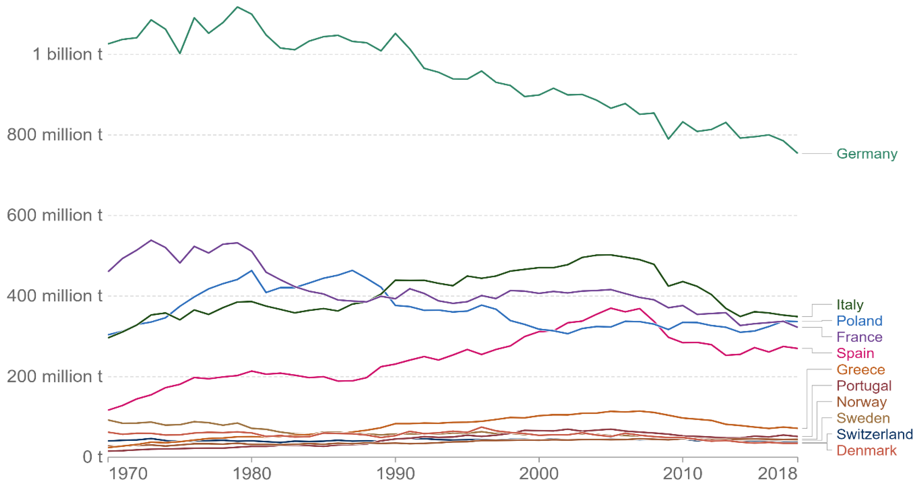
Figure 1. Annual growth of CO2 emissions in EU countries (source: Our World Data).
Energies 16 05885 g001
Figure 2. Time trend plots (source: authors’ own creation).
Energies 16 05885 g002
Figure 3. CUSUM and CUSUM-SQ.
Energies 16 05885 g003
Figure 4. Wavelet coherence between CO2 and GDP.
Energies 16 05885 g004
Figure 5. Wavelet coherence between CO2 and FDI.
Energies 16 05885 g005
Figure 6. Wavelet coherence between CO2 and OP.
Energies 16 05885 g006
Figure 7. Wavelet coherence between CO2 and EXP.
Energies 16 05885 g007
Figure 8. Wavelet coherence between CO2 and EC.
Energies 16 05885 g008
Table 1. Summary of studies on EKC hypothesis.
Author(s)SampleTime PeriodMethodsOutcomes
[40]Turkey1961–2010 ARDL EKC
[22]Pakistan1971–2014ARDL, NARDLEKC
[26]USA1960–2010ARDLEKC
[25]Turkey1971–2014ARDLEKC
[41]Europe1960–2005ARDL, VECMEKC for Italy and Denmark
[42]Turkey1960–2013ARDL, VECMEKC
[43]European countries1980–2014Panel OLS, FMOLS, FENo EKC
[44]Nigeria1971–2015ARDLEKC
[45]BRICS1980–2016CCEMG techniqueEKC
[46]GCC countries1980–2017STIRPAT model, PMGEKC
Note: ARDL: autoregressive distributed lag model. NARDL: nonlinear ARDL. VECM: Vector error correction model. OLS: ordinary least square. PMG: pooled mean group. EKC: environmental Kuznets curve. FMOLS: fully modified ordinary least square. CCEMG: common correlated effects mean group. STIRPAT: stochastic impacts by regression on population, affluence, and technology. FE: fixed effect.
Table 2. Data explanation and sources.
VariablesSymbolMeasurementSourcesReferences
Carbon emissionCO2Metric tons per capitaWorld Bank[31]
Gross domestic productGDPConstant 2010 US$ per capitaWorld Bank[45]
Foreign direct investmentFDIPer capita inflow of FDIUNCTAD[22]
Oil priceOPPer barrelStatista[22]
Energy consumptionECPer capita (million tons oil equivalent)British Petroleum Statistical Review[52]
ExportsEXPPer capita constant 2010 US$ World Bank[23]
Table 3. Descriptive statistics.
LCO2LGDPLFDILOPLECLEXP
Mean1.92010.2964.2123.1714.7403.108
Median1.91510.3864.3083.2454.7203.108
Max.2.10610.5526.6154.6954.9123.450
Min.1.6629.7800.4350.1914.5412.719
Std. dev.0.1160.2301.6461.0260.0970.195
Skewness−0.170−0.828−0.315−0.9750.259−0.108
Kurtosis2.1042.4072.0884.2602.0502.146
Jarque-Bera1.9156.4502.45511.2302.3391.617
Probability0.0390.2930.0040.2740.2620.446
Obs505050505050
Table 4. Correlation matrix.
LCO2LGDPLFDILOPLECLEXP
LCO21.000
LGDP0.4641.000
LFDI0.2470.7941.000
LOP0.0910.7540.5401.000
LEC0.8880.7420.5210.3611.000
LEXP−0.0170.7390.6170.8030.3411.000
Table 5. Unit root tests.
ADFPP
VariablesLevelFirst DifferenceLevelFirst Difference
LCO2−1.409−6.189 ***−1.471−6.187 ***
LGDP−1.144−6.180 ***−0.754−6.185 ***
LGDP-SQ−1.082−6.080 ***−0.683−6.086 ***
LFDI−3.150−3.423 *−6.152−34.610 ***
LOP−2.922−6.476 ***−2.937−6.465 ***
LEC−0.939−5.448 ***−1.123−5.429 ***
LEXP−2.492−6.688 ***−2.492−6.693 ***
Notes: *** p < 0.01, * p < 0.1.
Table 6. Zivot and Andrews structural break unit root test.
VariablesLevelFirst Difference
Test StatisticBreak YearTest StatisticBreak Year
LCO2−0.3192007−5.145 ***2007
LGDP−3.5061999−5.881 ***1980
LGDP-SQ−3.5961999−5.145 ***1991
LFDI−0.6551983−21.817 ***2012
LOP−1.4371981−6.933 ***1980
LEC−1.8062006−5.998 ***2014
LEXP−2.8071978−7.675 ***2009
Notes: *** p < 0.01.
Table 7. Bounds test estimates.
F-StatisticsH0: No Level Relationship
SignificanceI(0)I(1)
Optimal lag-length
F-statistics
(3, 3, 3, 2, 3, 3, 2)
12.791 ***10%1.992.94
K65%2.273.28
2.50%2.553.61
1%2.883.99
Notes: *** p < 0.01.
Table 8. ARDL long-run results.
Dependent VariableRegressorsCoefficientsStd. Errort-Statistics
LCO2LGDP14.8913.8793.839 ***
LGDP-SQ−0.7400.192−3.852 ***
LFDI0.0390.0075.271 **
LOP−0.0270.008−3.289 ***
LEC0.5250.1703.085 **
LEXP0.0810.0382.138 **
Notes: *** p < 0.01, ** p < 0.05.
Table 9. ARDL short-run results.
Dependent VariableRegressorsCoefficientsStd. Errort-Statistics
LCO2LGDP35.5284.0128.855 ***
LGDP-SQ−1.7130.198−8.638 ***
LFDI0.0100.0016.915 **
LOP−0.0410.006−7.075 ***
LEC0.6630.0788.458 ***
LEXP0.0710.0262.768 **
Coint. Eq. (−1)−0.3610.318−11.351 ***
Notes: *** p < 0.01, ** p < 0.05.
Table 10. Dynamics OLS results.
VariablesCoeff.Std. Errort-Statp-Value
LGDP100.232 ***15.8816.3110.024
LGDP-SQ−5.002 **0.789−6.3390.024
LFDI0.235 **0.0405.8060.028
LOP−0.153 **0.030−5.0350.037
LEC1.754 ***0.9618.2480.003
LEXP0.888 **0.1267.0640.019
Notes: *** p < 0.01, ** p < 0.05.
Table 11. Fully modified OLS results.
VariablesCoefficientsStd. Errort-StatisticProbability
LGDP32.969 ***1.24326.5340.000
LGDP-SQ−1.644 ***0.061−26.7680.000
LFDI0.072 ***0.00234.9930.000
LOP−0.079 ***0.003−20.2390.000
LEC1.603 ***0.03742.7120.000
LEXP0.039 *0.0201.9260.061
Notes: *** p < 0.01, * p < 0.1.
Table 12. Diagnostics tests statistics.
Diagnostics TestsX2p-ValueDecision
Breusch-Godfrey LM0.9860.473No issue with serial correlation
Breusch-Pagan-Godfrey0.7030.776No issue with Heteroscedasticity
ARCH test0.0190.889No issue with Heteroscedasticity
Normality3.7080.157Estimated residuals are normal
CUSUM and CUSUM-SQ Stable
Disclaimer/Publisher’s Note: The statements, opinions and data contained in all publications are solely those of the individual author(s) and contributor(s) and not of MDPI and/or the editor(s). MDPI and/or the editor(s) disclaim responsibility for any injury to people or property resulting from any ideas, methods, instructions or products referred to in the content.