Abstract
The amount if oil shale resources throughout the world has been roughly estimated in accordance with various resource estimation methods. However, in some instances, detailed and comprehensive supporting methodologies for the estimation of commercial shale oil reserves have not been presented. The goal of this study is to develop a comprehensive method for the modified estimation of oil shale mineable reserves for shale oil projects. The methodology characterises oil shale according to its calorific value, oil content, conditional organic mass, and ash content by utilising a Monte Carlo simulation. Based on the results of the case study, the developed method proposes considering the relationships of the in situ oil shale grade and tonnage material (oil shale + limestone) to the oil retorting feed material grade and tonnage by taking into account the retorting plant oil recovery. For this purpose, a Monte Carlo stochastic modelling algorithm was developed. Based on the data analysis, a modifying factor to convert mineral reserves to petroleum reserves was produced. The results of this study are useful for feasibility studies that estimate oil shale reserves in relation to justifying their utilisation fields. Some oil shale deposits have good potential for development but need to be re-estimated in accordance with the most sophisticated extraction and processing technologies.
1. Introduction
The amount of oil shale resources throughout the world has been roughly estimated in accordance with various resources estimation methods; however, in some instances, detailed and comprehensive supporting methodologies for the estimation of commercial shale oil reserves have still not been presented. Estimating oil shale reserves is an important topic for the oil industry as it affects the future global energy balance, pricing, and energy security. The estimation of oil shale reserves has become a topic of significant interest in recent years due to the increasing demand for energy [1]. However, there are many uncertainties regarding reserve estimation for many oil shale deposits. Until now, all attempts to estimate the world oil shale resources have been based on numerically insignificant facts, and estimations of the grade and tonnage of many of these materials were, at best, guesswork [1,2]. Stephen et al. presented some methods for the calculation and reporting of oil shale resources. Their study demonstrated that “a more uniform system of reporting resources of oil shale deposits is desirable to enable an accountable and reliable estimate of resources to be made”. Their study emphasised the importance of determining the level of confidence of resource estimates [2].
The problem of estimating shale oil reserves while receiving the maximum economic profit and producing minimal environmental and social impacts is becoming increasingly urgent. The traditional reserve estimation methods do not address specific technical aspects of modifying factors; thus, they are not able to solve the problem of converting solid minerals into oil [3,4,5,6,7,8,9,10,11,12,13,14,15,16,17,18,19]. Few of the existing research methodologies are able to accurately estimate shale oil reserves based on solid mineral material. In most cases, shale oil resources (referred to as “reserves”) are estimated based on the laboratory Fisher assay oil yield percentage of the tested material [5,6,7]. This can serve as a conceptual estimate only for oil resources and not for oil reserves, the recovery of which requires the use of modifying factors [6,7,8,9]. One of the objectives of this study is to produce a modifying factor capable of converting mineral reserves to petroleum reserves.
Oil shale, a sedimentary rock containing kerogen, has been identified as a potential alternative source of fuel. However, accurately estimating the amount of oil that can be extracted from shale is a challenging task due to the complex nature of the rock and the lack of extensive production history in many shale oil ventures [3,4,5,6,7,8,9,10,11,12].
Currently, oil shale reserve estimations are proposed by the mineral reserve estimate method and oil reserve estimate method. The mineral reserve method assumes a project producing power, and oil reserves presuppose a project for producing oil and chemical products. In both estimation methods, the amount of oil underground is presented as reserves or resources depending on how and when this amount will be extracted or excavated using the available technologies [13,14]. Thus, oil reserves have to be considered according to technical and economic feasibility. Oil reserves estimates are typically presented via probability distributions because of uncertainties in geology, technology, and economics. There are three levels of confidence, namely proved (1P), proved and probable (2P) and proved, probable, and possible (3P) in the petroleum classification system. The level of proved and probable is used in the mineral classification system. A comparison of the mineral and petroleum reserve systems is presented in Figure 1 [13,14].
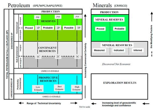
Figure 1.
Comparison of petroleum and mineral classification systems (CRIRSCO).
Generally, mineral and petroleum reserves are the same as they are ready to be extracted or excavated using the available technologies, producing saleable products. The only difference is that the mineral reporting code does not establish any specific time restrictions, while the petroleum reporting code requires extraction to be started within a “reasonable” timeframe [13,14].
To derive mineral reserves from mineral resources, modifying factors should be used. These cover mining considerations (i.e., the cut-off grade, losses and dilutions, etc.), processing, metallurgical, infrastructure, economic, marketing, legal, environment, social and government factors. They are known as “contingencies” in the petroleum industry. Mineral reserve estimation is typically presented in terms of tonnes of ore and grade for both the run-of-mine and saleable product after the beneficiation. Mineral reserve statement should include disclosure on the recovery factors used for reserves to receive saleable product quantities. The petroleum report code normally derives oil reserves as a more refined saleable product (e.g., oil with very minor non-hydrocarbons or sulphur) [13,14].
Biglarbigi et al. (2010) in “Rethinking World Oil-Shale Resource Estimates” challenged the conventional estimation of oil shale resources by highlighting that the current estimation does not account for the technological advancements in extraction and processing techniques. The study pointed out that the actual reserve estimations could be much higher than the conventional ones, which are based on outdated technology. They suggested that the industry should invest in further research and development to unlock the true potential of oil shale resources [15].
Knaus et al. (2010) in “An Overview of Oil Shale Resources” provided an overview of the global oil shale resources, the technologies used for oil extraction, and its economic viability. The study highlighted that the oil shale industry faces several challenges such as high production costs, environmental concerns, and technical limitations. The authors concluded that oil shale resources could be an important contributor to the future energy but require further technological advancements and investments to become economically viable [16].
McGlade (2012) in “A review of the uncertainties in estimates of global oil resources” conducted a critical review of the estimations of global oil resources, including oil shale reserves. The study highlighted the level of uncertainty in the estimations due to various factors such as geological complexity, political instability, and the lack of transparency in reporting. The author suggested that a better understanding of these uncertainties is necessary to advise energy policies and investment decisions [17].
Xu et al. (2022) in “Occurrence space and state of shale oil: A review” reviewed the current state of knowledge on shale oil, including its geology, extraction technologies, and production characteristics. The study highlighted the complexity of shale oil resources, including their heterogeneity, low permeability, and variability in oil quality. The authors suggested that further research is necessary to better understand the distribution and condition of shale oil resources to improve the accuracy of their estimation [18].
Smith (2018) in “Estimating the future supply of shale oil: A Bakken case study” examined the supply potential of the Bakken shale formation in North Dakota, USA. The study used a production forecasting model to estimate the future production of oil from the Bakken formation. The study found that the Bakken formation has a significant oil resource potential, but there is a substantial drop in the production rate, and the production economics are sensitive to oil prices [19].
Gong et al. (2013) in “Assessment of Eagle Ford Shale Oil and Gas Resources” conducted an assessment of the Eagle Ford shale formation in Texas, USA. The study used a combination of reservoir engineering and geologic analysis to estimate the amount of oil and gas resources in the formation. The study found that the Eagle Ford formation has a significant oil and gas resource potential, and the production economics are favourable due to the high-quality reservoir characteristics [20].
Misund and Osmundsen investigated the relationship between different classifications of reserves and total shareholder returns for oil and gas companies. They discovered that, despite the fact that proven developed reserves are the ones that the investors should use to anticipate future cash flows, there are discrepancies in the pricing of oil and gas reserves, particularly after 2009 because of the shale gas revolution. The authors suggest that the impact of the shale oil boom and the subsequent oil price slump may have affected the valuation of the oil and gas companies. They also argue that mandatory disclosure of reserve classifications, including probable reserves, potentially increase the attention that investors and analysts pay to this information and have policy implications for oil and gas companies, particularly those listed in the US [21].
Additionally, it should be noted that emphasis should be given to unconventional technologies, such as shale gas hydraulic fracturing and oil shale in situ conversion (retorting) while evaluating the various techniques used to assess oil shale reserves. In the in situ conversion process, an electric resistance heating slowly heats the shale to the temperature of kerogen conversion, ready to be pumped from the ground [22,23]. Hydraulic fracturing is a technical means to realise the efficient development of shale gas. Hydraulic fracturing is used to increase oil and gas production from oil reservoirs. Hydraulic fracturing involves injecting water and chemicals under high pressure into a shale formation throughout wells to create new fractures and increase the connectivity of the existing fractures in order to extract oil and gas. This method could be helpful for enhancing oil recovery and may serve to improve reserve estimation approaches [24,25,26,27,28].
All of the above shows that the estimates of oil shale reserves are subject to significant uncertainty due to various factors such as geological complexity, technological limitations, and economic viability. The studies suggest that further research and investment in technology are necessary to unlock the full potential of oil shale resources and provide a more accurate estimation of shale oil reserves.
More than 550 of the known oil shale deposits worldwide are distributed in over 50 countries. According to Knaus (2010), an oil shale is formed from organic material that may have several different origins. Oil shale is often categorised into three major types according to the origin of the organic material: terrestrial, lacustrine, and marine. Marine (e.g., kukersite, tasmanite, and marinite) oil shale deposits, which are more often used in the industry, are the result of saltwater algae, acritarchs, and dinoflagellates [16]. The kukersite formation is located in Estonia and has been developing over the last hundred years.
Raukas and Punning (2008) stated that oil shales are defined as sedimentary rocks containing 10–75% of organic matter [29]. The organic matter is characterised by its elemental composition. An important indicator of oil content in organic matter is the ratio of hydrogen (H) to carbon (C) (i.e., the H/C) [30]. Oil yield is dependent on not only H/C but also the initial material of the organic matter and its degree of decomposition. The mineral part of oil shale may consist of terrigenous material, carbonates, or both. The terrigenous material is mainly composed of clay and supplemented by quartz and feldspars. Carbonates are represented by calcium carbonate (calcite) and, in some cases, dolomite [31,32,33,34,35].
Oil shale deposits may also contain metals, which could add some byproducts such as alum [KAl (SO4)2·12H2O], nahcolite (NaHCO3), dawsonite [Na(Al(OH)2CO3], sulfur, ammonium sulfate, vanadium, zinc, copper, and uranium, and others [1].
Oil shales are situated at several depths, and their operational seams have variable thicknesses. An oil shale can be mined either by surface or underground methods, as well as by in situ retorting technologies [22,23,24]. For the mining of oil shale deposits, location, geological structure, bed thickness, depth and orientation, grade and tonnages, deposit type, and other aspects should be considered [10].
Considering all these critical issues mentioned above, the main goal of this study is to develop a comprehensive method for the modified estimation of oil shale mineable reserves for shale oil projects. For this study, data for over 96 oil shale deposits located in 23 countries were analysed. A consolidated commercial estimation criteria characterising oil shale reserves considering their quality by calorific value, oil content, organic mass, and ash content were used in the methodology. These criteria are based on the aggregated values proposed for commercial (mineable) oil shale seams (beds) and not just for separately tested oil shale layers. The developed methods provide oil recovery outcomes based on industrial data that can be used for feasibility studies, which require demonstrating a project economy estimated on a practical commercial database.
2. Materials and Methods
Wang et al. concluded that “the Monte Carlo method is a statistical test method that can be used to solve mathematical physics problems in which it is difficult to determine the most appropriate equation through statistical sampling theory” [36]. Ni suggested that “for a variable with a specific uncertainty probability density function, the Monte Carlo method provides an easier solution to the synthetic uncertainty that approaches the real solution” [37]. Monte Carlo simulation is a broad term for computational algorithms that generate random numbers (realisations) given a specific density function, as per the Pyrcz and Deutsch study [38]. Deutsch and Journel report on the Monte Carlo simulation of random numbers from an arbitrary probability or cumulative distribution function [39]. According to the ergodic theory [40] researched by Chile and Delfiner, a large number of values must normally be simulated in order for the statistical characteristics (such as the mean and variance) of the simulated values to converge to those of the original dataset. When cash flows are sampled across a range of costs, a Monte Carlo simulation can show how nonlinearity and path dependence affect the estimated cash flow levels.
Monte Carlo modelling has been used in our study to demonstrate a range of possible outcomes because our database was generated based on variable values that are not suitable for deterministic modelling.
To estimate oil shale reserves, it is necessary to identify a reasonable saleable product, i.e., for power production, which could be based on calorific value, or for fuel or chemical products, which are based on oil yield [31,32,33,34,35]. Current methodologies for estimation of mineable reserves for the oil shale project do not consider particularly modifying factors to convert solid mineral reserves to oil reserves. Petroleum and mineral reporting codes assume only conversion between their named “Proved” and “Probable” reserves but do not propose the relationship of calorific values with the oil content. For a detailed numerical analysis, oil shale mineral part chemical composition (e.g., SiO2, Al2O3, Fe2O3, TiO2, CaO, MgO, SO3, K2O, Na2O, P2O5) and kerogen oil elemental composition (e.g., H, C, S, N, O, H/C) can be considered [4,5,6,7,8,9,10,11,12]. Ash and sulphur content are key parameters for choosing the oil-refining technology [4,5,6,7].
Thus, to estimate oil shale mineable reserves for shale oil projects, the following algorithm for the research methodology is proposed:
- Analysis of oil shale properties and characteristics, including calorific value, ash content, oil content, and semicoke.
- Analysis of the correlation coefficient (Figure 2) for oil content vs. semicoke “(A)” and oil shale conditional organic mass vs. ash content “(B)” with the help of a peer-reviewed database (Appendix A) of oil shale deposits around the world.
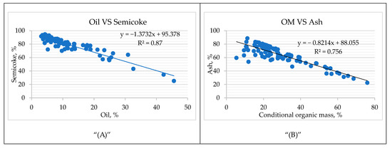 Figure 2. Correlation coefficients of oil vs. semicoke (A) and conditional organic mass (OM) vs. ash (B).
 - Stochastic modelling with the help of Monte Carlo simulation considering
- Oil content and conditional organic mass distributions;
- Estimation of the variability of the oil content and the productive oil shale seam thickness;
- Estimation of recovered oil from the commercial oil shale seam with variation of oil in the seam, the seam utilisation factor, and processing recoveries.
- Analysis of the correlation coefficient for oil content vs. calorific value from the peer-reviewed database.
- Stochastic modelling for variations in oil content distribution at the particular calorific value.
Figure 2 presents the relationships between oil content and semicoke and between conditional organic mass and ash content.
This demonstrates that most oil shale projects are in the range of 5–20% oil content and require reasonable technologies for re-handling semicoke products.
The average chemical composition of the oil shale mineral part is presented in Figure 3.
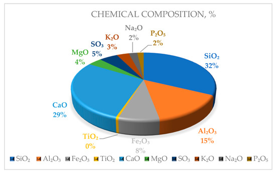
Figure 3.
Chemical composition of oil shale mineral part.
These relationships can be used as a basis for the conversion of oil shale mineral reserves to shale oil reserves and vice versa.
For this study, a Monte Carlo simulation is proposed to be used for building models demonstrating possible outcomes. For producing the models, any uncertainty factor is replaced by a range of values, which is called the distribution of probability. After that, numerous computations of the outcomes are produced, at every turn establishing a variety of stochastic variables for the probability functions. Monte Carlo modelling helps to determine the value distribution of the probable numbers with several likely outcome values. For this study, Monte Carlo modelling uses input results from Triangle and Program Evaluation and Review Technique (PERT) distributions [41,42,43]. For the simulation of the oil content and the conditional organic mass, as a major variability, a triangle distribution for min, max, and most likely (weighted average) values was utilised. In the simulation, 10,000 iterations were used.
Figure 4 demonstrates the modelling outcomes for the oil content and conditional organic mass (COM) from 96 analysed oil shale deposits, showing that they ranged from 7.5% to 37.2% for oil and from 18.7% to 74% for COM at 90% confidence levels.
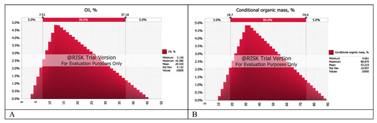
Figure 4.
Oil content (A) and conditional organic mass (B) distributions.
The PERT distribution can be used for event impact estimation (i.e., severity). For the case study, the PERT distribution is applied to estimate the oil shale retorting recoveries based on the historically derived minimum, most likely, and maximum values, and also to estimate a potential oil content in relation to calorific values [41,42,43].
3. Results
3.1. The Case Study Mine
An oil shale called “Kukersite” was formed during the early Upper Ordovician times, about 460 million years ago. The oil shales have been successfully developed over the last hundred years for use in producing power, shale oil, heating, and some chemical products [9,10,29,30,31,32,33,34].
The study mine employs large-scale room and pillar mining that produces oil shale via conventional drilling and blasting followed by mucking to conveyors, which transport oil shale to a beneficiation plant located on the ground surface. Beneficiation is used to separate oil shale from waste rock (limestone) by applying crushing, sieving, and a dense media suspension approach. Mines use room-and-pillar mining methods, which account for 30–40% of oil shale losses. The overburden is a consequence of limestone. Local oil shale is composed of stratified sedimentary rock rich in organic matter (15–46% kerogen, 26–57% carbonates, and 18–42% clastic materials). Within tectonic dislocation zones, the karst clay content is about 10–15%. Fractured zones are typically abundant in water and unstable. The rock in the fractured zones is dolomitised and contains some calcite and pyrite veins, sometimes with marcasite, galena, sphalerite, and barite [9,10,29,30,31,32,33,34].
The mined oil shale seam comprises thin layers of oil shale together with thin intervening layers of low calorific limestone. This material, together with some roof and floor strata (which are unavoidably worked as part of the extraction process), is referred to as the Run-of-Mine Product (RoM). Enrichment plants process the RoM into a Retorting Feed Product (RF) by removing most of the limestone and achieving the required calorific value for the retorting process. Oil shale retorting plants require certain feed qualities for processing oil shale with optimum efficiency. The processing plants using the Galoter technology required a feed grade of 16% oil content at a size of 0–25 mm [5,6,7,8].
Horizontal retort with a solid heat carrier is named the Galoter type of Retort (Petroter, Enefit, Petrosix, etc.). The Galoter Retort technology uses a pyrolysis (semi-coking) process for the processing of fine shale (fractional content from 0 to 25 mm) with a solid heat carrier. Through a mixture of oil shale and heated ash in the absence of air, the heating and (by sufficient temperature) destruction of organic matter contained in oil shale occur, followed by the emission of liquids and gases [5,8].
The gas–vapor mixture generated in the reactor over the pyrolysis process passes through several treatments for cleaning from ash and solid particles and comes to the distillation process for the production of liquid products and high-calorific gas. The Galoter technology is designed for the thermal decomposition (pyrolysis) of fine-grained oil shale with the objective of producing shale oils, gas with a high calorific value, and high-pressure steam. The oil shale pyrolysis process is effected in a drum rotating reactor in the absence of air at a temperature of 450–500 °C due to the mixture of oil shale with hot ash (as a solid heat carrier). Liquid products are fed to other units for loading as final products or for further processing. Gas is fed to the heat power plant for heat and power production. Steam is fed to the heat power plant for power production. The by-products of this process include phenol water, flue gases, and ash from thermal processing [5,8].
The RF resulting from these processes is then transported to the retorting plant at a consistent calorific value of 8.4 MJ/kg, or 2007 kcal/kg. This is the product that takes into account the reduction in tonnage and increase in calorific value following the enrichment process through the beneficiation plant. The commercial oil shale seam, or RoM, consists of six oil shale layers specified from bottom to top by indexes A, B, C, D, E, F1, F2, F3, and four interbedded limestone layers designated as A/B, B/C, C/D, D/E, F1/F2, and F2/F3 (Table 1). Oil shale uniaxial compressive strength is measured at 18–40 MPa, and that for limestone is measured at 65–82 MPa (Table 1). The volume density of these rocks varies from 1.2 to 1.7 t/m3 and from 2.1 to 2.5 t/m3, respectively. Young module for layer “C” is E~7.1 GPa and σr ~2.5 MPa [8,10,44].

Table 1.
Commercial oil shale seam properties.
3.2. Analysis of Oil Shale Seam Properties
Layers from A to F3 are extracted as a single unit (the commercial oil shale seam, “CS”) of an approximately 3.86 m thickness for our case study underground mine (Table 1).
Oil content is related to the oil shale commercial seams shown in Figure 4A. Oil content is estimated for the top of the oil shale seam on a composite layer thickness basis and takes into account only oil shale layers without considering low-grade limestone material. Based on the data from Table 1, the oil shale can be mined with different seam thicknesses. Variations of these thicknesses offer it various contents. Figure 5B demonstrates possible outcomes for the commercial oil shale seam thickness that lies in a range of 2.6–3.8 m, which corresponds to historical mining thicknesses.
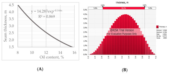
Figure 5.
Variability of oil content (A) and productive oil shale seam thickness (B).
Based on our case study data, the commercial seam thickness and oil content in it can be estimated by the following formula:
where H is the seam thickness, OC—oil content.
H = 14.287exp−0.144∗OC,
3.3. Monte Carlo Simulation
For the simulation of the oil content in the commercial seam as a main variability, a triangle distribution is utilised, and for Seam Utilisation and Reporting Recoveries, a PERT distribution for min, max, and weighted average values is utilised (Figure 6). In Figure 6A, all layers, including low-grade limestone material are considered. These outcomes should be taken into account while considering the beneficiation process. Figure 6B demonstrates the outcomes only for oil shale layers that are processed to achieve the required retorting feed grade of 16%. Figure 6C demonstrates oil shale seam utilisation (SU), which is the volume of limestone layers divided by oil shale layers. The retorting plant recoveries based on historical data are shown in Figure 6D.
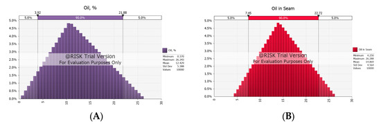
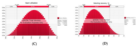
Figure 6.
Oil yield from the commercial oil shale seam.
It should be noted that this shale oil is not a final product and it requires additional refinery processes to produce final saleable oil and chemical products.
Based on our case study, the developed method proposes to consider relationships of in situ (RoM) grade and tonnage material (waste + oil shale) to the beneficiated material (Retorting Feed Product) grade and tonnage which is actually the Seam Utilisation (SU) factor, and to take into account the retorting plant recoveries (RR):
Recovered oil (kg) = RoM ∗ SU ∗ RR.
Using input parameters received from our case study, Monte Carlo modelling demonstrated that the recovered oil from the retorting process ranges from 57 to 69 kg per tonne of RoM material (Figure 7).
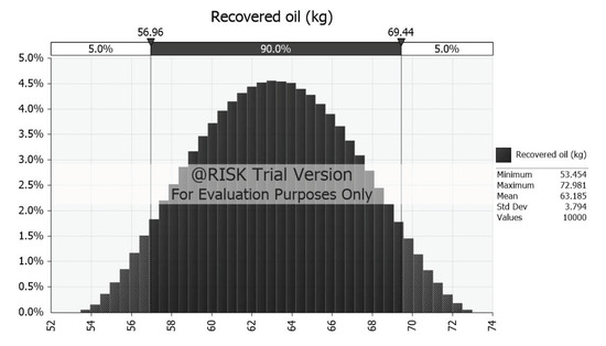
Figure 7.
Recovered oil.
4. Discussion
Zelenin and Ozerov suggested some industrial classification of oil shale, which involves the combination of estimation criteria characterising the industrial value of each type of oil shale by considering its quality. They proposed Sapropelic at a 12.5 MJ/kg oil content over 30%, Sapropelic–Humus at a 8.4–12.5 MJ/kg oil content 10–12%, and Humus–Sapropelic at a 6.3–8.4 MJ/kg oil content below 10% [12].
These proportions of oil content to calorific value are based on different types of oil shale and cannot be used for a good correlation analysis. Baukov derived relationships only between calorific value and density; Grabovskiy developed correlation coefficients for ash and calorific value but not in relation to oil content [11,12].
Reinsalu et al. [8,9] derived that the calorific value and oil content are in direct relation to the kerogen content. Kerogen’s calorific value is 35 ± 3 MJ/kg; thus, the oil shale calorific value formula is
where K is kerogen fraction (100% = 1), and its oil content formula is
Q = 35 K, MJ/kg,
T = 65.5 K = 1.86 Q %.
However, this formula can be valid only for the Kukersite type of oil shale based in Estonia.
For this study, calorific value and oil content data from the operational oil shale projects located in Estonia, China, and Brazil were analysed. Based on this analysis, the correlation coefficients for oil content and calorific value were produced (Figure 8). R2 = 0.9 shows a confident level of correlation.
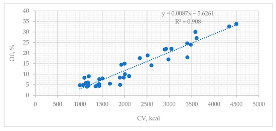
Figure 8.
Calorific Value vs. Oil content.
The received correlation coefficient between oil and calorific value can be used as a modifying factor in cases where oil shale deposits are estimated in accordance with Mineral Reserve codes and must be re-estimated to Petroleum (Oil) Reserves.
Oil = 0.0087 ∗ CV − 5.6261.
The Monte Carlo simulation shows that for oil shale, the calorific value varied from 1556 to 3949 kcal/kg, and the oil content lies between 8.2% and 28.6% for the derived relationship (Figure 9).
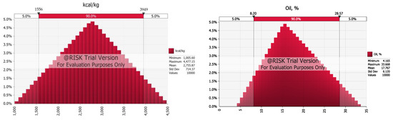
Figure 9.
Simulated calorific Value vs. Oil content.
The above-analysed data are recommended for stochastic modelling of possible outcomes for recoverable oil based on calorific value. For example, at a calorific value of 2000 kcal/kg, the Monte Carlo simulations show that it ranges from 9.6 to 13.8% (Figure 10).
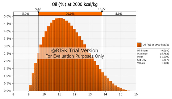
Figure 10.
Variation of oil content at 2000 kcal/kg.
Simulation results also demonstrated that there is only a 5% chance that the oil content will be less than 9% (Figure 10).
The proposed methodology will help examine oil shale reserves for shale oil projects. The derived modifying factor is capable of converting mineral reserves into petroleum reserves.
The results of this study may be useful for feasibility studies estimating oil shale quantity and quality in order to consider their utilisation area. Some oil shale deposits have good potential for development but need to be re-estimated in accordance with the most sophisticated extraction and processing technologies. According to this study, oil shale deposits can be characterised as having a suitable oil content and an appropriate heating value for industrial projects.
5. Conclusions
A comprehensive method for the modified estimation of oil shale mineable reserves for shale oil projects was developed. The study methodology analysed data from 96 worldwide oil shale deposits to develop consolidated commercial estimation criteria characterising oil shale by calorific value, oil content, conditional organic mass (COM), and ash content.
A case study on Kukersite type oil shale, which is used for the production of shale oil, power generation, and numerous chemical products, was produced. Based on the case study results, the developed method proposes to consider the relationships of in situ oil shale grade and tonnage material (oil shale + limestone) to the oil retorting feed material grade and tonnage by taking into account the retorting plant oil recovery. Using these as input parameters, a Monte Carlo simulation derived the likely results for the recovered oil from the retorting process and demonstrated that it ranged from 57 to 69 kg per tonne of RoM material. For this, a Monte Carlo stochastic modelling algorithm was developed.
From commercial oil shale characteristic data analysis, the correlation coefficient between oil and calorific value was received: Oil = 0.0087 ∗ CV − 5.6261.
This correlation can be used as a modifying factor to convert mineral reserves to petroleum reserves.
These specific practical numerical results can be applied to testing various oil shale deposits. The results of this study are useful for feasibility studies estimating oil shale quantity and quality in relation to justifying their utilisation. Several oil shale deposits might have potential for extraction but need to be re-estimated in accordance with the most sophisticated development and processing methods.
The results obtained in this case study on the specific production facilities and based on a database from 96 oil shale deposits are prospective for use in various regions and are prospective for the countries in which the data was used for analysis.
Author Contributions
Conceptualisation, S.S.; methodology, S.S.; software, S.S.; validation, S.S.; formal analysis, S.S.; investigation, S.S.; resources, S.S.; data curation, S.S.; writing—original draft preparation, S.S., A.R.Q., Z.D. and G.K.; writing—review and editing, S.S.; visualisation, S.S.; supervision, S.S.; project administration, S.S.; funding acquisition, S.S. All authors have read and agreed to the published version of the manuscript.
Funding
This research was funded by Nazarbayev University Grant Programs: Research Grant #20122022FD4128 and Collaborative Research Project #091019CRP2104.
Data Availability Statement
Data available on request due to privacy restrictions. The data presented in this study are available on request from the corresponding author. The data are not publicly available due to confidentiality agreements between parties.
Acknowledgments
This study is supported by Nazarbayev University Grant Programs: Research Grant #20122022FD4128 and Collaborative Research Project #091019CRP2104.
Conflicts of Interest
The authors declare no conflict of interest.
Correction Statement
This article has been republished with a minor correction to the Funding statement. This change does not affect the scientific content of the article.
Appendix A
| # | Name | Ash, % | Conditional Organic Mass, % | Oil, % | Semicoke, % |
| 1 | Olenyek (Russia, Yakutia) | 6.9 | 87.7 | ||
| 2 | Kvarntorp (Sweden) | 79 | 20.0 | 6.7 | 86.4 |
| 3 | Kukersite (Estonia) | 46.5 | 35.5 | 23.3 | 71.0 |
| 4 | Tetraspis (Estonia) | 79 | 15.2 | 6.4 | 89.9 |
| 5 | Ashinsk (Russia, Bashkiria) | 69.7 | 14.8 | 6.3 | 90.2 |
| 6 | Turovo (Byelorussia) | 70.1 | 17.2 | 8.6 | 87.1 |
| 7 | Lyuban (Byelorussia) | 71.1 | 11.7 | 6.3 | 90.2 |
| 8 | Ukhta (Russia, Komyi) | 76.4 | 10.6 | 4.3 | 94.6 |
| 9 | Chernozatonsk (Kazakhstan) | 36.2 | 54.0 | 22.8 | 57.4 |
| 10 | Lemeza (Russia, Bashkiria) | 72.1 | 27.7 | ||
| 11 | Selenyakh (Russia, Yakutia) | 53.7 | 11.9 | ||
| 12 | Antrim (USA) | 82.6 | 16.7 | 3.7 | 90.4 |
| 13 | Westwood (Geat Britain, Scotland) | 77.8 | 19.0 | 8.2 | 86.6 |
| 14 | New Glasgow (Canada) | 76.9 | 18.8 | 5.3 | 88.7 |
| 15 | Nova Scotia (Canada) | 62.4 | 34.4 | 18.8 | 77.7 |
| 16 | Ermelo (South Africa) | 44 | 54.2 | 17.6 | 75.6 |
| 17 | Kenderlyk, the Kalyn-Kara seam (Kazakhstan) | 51.6 | 48.4 | 9.7 | 70.0 |
| 18 | Kenderlyk, the Karaungur seam (Kazakhstan) | 76.4 | 21.7 | 13.6 | 76.7 |
| 19 | Kenderlyk, the Saikan seam (Kazakhstan) | 77.2 | 22.0 | ||
| 20 | Ust-Kamenogorsk (Kazakhstan) | 74 | 22.8 | 8.0 | 84.0 |
| 21 | Pashin (Russia, Perm District) | 73.4 | 26.5 | 6.0 | 86.4 |
| 22 | Glen Davis (Australia) | 51.6 | 48.4 | 30.9 | 64.1 |
| 23 | Puertollano (Spain) | 63 | 35.0 | 17.8 | 78.4 |
| 24 | Irati (Brazil) | 64.2 | 34.0 | 10.8 | 82.6 |
| 25 | Otain (France) | 73.7 | 19.8 | 8.2 | 87.2 |
| 26 | St.-Hilaire (France) | 69.3 | 27.3 | 9.5 | 85.9 |
| 27 | Cerro Largo (Uruguay) | 78.4 | 21.6 | 4.2 | 81.6 |
| 28 | Verkhnetutonchansk (Russia, Krasnoyarsk District) | 31.2 | 63.3 | ||
| 29 | Omolon, Astronomicheskaya River region (Russia) | 78.3 | 21.5 | ||
| 30 | Omolon, Levyi Kedon River region (Russia) | 82.2 | 17.6 | ||
| 31 | Bogoslov, seam II (Russia, Yekaterinburg District) | 36.1 | 60.9 | 21.9 | 62.8 |
| 32 | Alyouisk (Russia, Irkutsk District) | 60.8 | 38.9 | 9.2 | 81.7 |
| 33 | Budagovo, (Russia, Irkutsk District) | 45.6 | 25.2 | ||
| 34 | Budagovo, humic sapropelite (Russia, Irkutsk District) | 28.5 | 68.6 | 5.2 | 72.0 |
| 35 | Budagovo, humic sapropelite (Russia, Irkutsk District) | 52 | 42.8 | 18.9 | 72.1 |
| 36 | Bouinsk (Russia, Tatarstan) | 65 | 24.0 | 8.5 | 76.9 |
| 37 | Voronye-Voloskovsk (Russia, Vyatka District) | 75.3 | 20.1 | 5.7 | 87.5 |
| 38 | Würtenberg (Germany) | 70.8 | 9.5 | 4.5 | 94.0 |
| 39 | Sysol, Ibsk deposit (Russia, Komyi) | 72.7 | 21.4 | 7.7 | 76.8 |
| 40 | Kashpir (Russia, the Volga oil shale basin) | 58.2 | 30.5 | 12.0 | 79.8 |
| 41 | Kimmeridge (Great Britain, England) | 37.7 | 59.8 | 25.5 | 60.2 |
| 42 | Levosviyazh (Russia, Tatarstan) | 68.3 | 23.4 | 8.8 | 81.4 |
| 43 | Manturovo (Russia, Nyzni Novgorod district) | 57.3 | 39.2 | 12.9 | 72.0 |
| 44 | ObshchiSyrt, seam P3A (Russia, the Volga oil shale basin) | 56.2 | 33.8 | 11.6 | 73.7 |
| 45 | Perelyub-Blagodatsk (Russia, the Volga oil shale basin) | 47.2 | 45.6 | ||
| 46 | Simbirsk (Russia, the Volga oil shale basin) | 62 | 31.9 | 9.2 | 81.2 |
| 47 | Kharanor (Russia, Chita District) | 76.4 | 23.6 | 6.4 | 88.0 |
| 48 | Khakhareisk, boghead (Russia, Irkutsk District) | 42.3 | 34.5 | ||
| 49 | Khakhareisk, oil shale (Russia, Irkutsk District) | 43.9 | 56.1 | 11.4 | 76.9 |
| 50 | Chagan (Russia, Orenburg District) | 35.7 | 56.7 | 24.9 | 56.0 |
| 51 | Sysol, Poingsk region (Russia, Komyi) | 66.8 | 27.9 | ||
| 52 | Savelyev (Russia, the Volga oil shale basin) | 61.4 | 27.8 | 10.5 | 80.5 |
| 53 | Yarenga (Russia, Komyi) | 22.4 | 76.0 | 32.6 | 43.2 |
| 54 | Nebi Musa (Jordan) | 63.1 | 22.0 | 13.6 | 80.4 |
| 55 | Olenyek, boghead (Russia, Jakutia) | ||||
| 56 | Timahdit (Morocco) | 68.8 | 23.1 | 5.6 | 92.9 |
| 57 | Um-Barek (Israel) | 57.2 | 24.7 | 6.4 | 88.4 |
| 58 | Efyie (Israel) | 56.1 | 23.9 | 7.6 | 87.9 |
| 59 | Baisun (Uzbekistan) | 55.2 | 38.0 | 13.5 | 73.3 |
| 60 | Eastern Chandyr (Uzbekistan) | 66.1 | 18.8 | 5.0 | 85.0 |
| 61 | Eastern Urtabulak (Uzbekistan) | 53.9 | 39.8 | 10.6 | 72.3 |
| 62 | Kapali (Uzbekistan) | 60.1 | 29.7 | 7.6 | 83.8 |
| 63 | Kultak-Zevardy (Uzbekistan) | 62.6 | 22.8 | 6.2 | 83.0 |
| 64 | Pamuk (Uzbekistan) | 63.7 | 15.6 | 3.7 | 87.3 |
| 65 | Sangruntau (Uzbekistan) | 74.8 | 23.9 | 6.1 | 84.9 |
| 66 | Todinsk (Uzbekistan) | 65.7 | 27.8 | ||
| 67 | Shurasan (Uzbekistan) | 63.2 | 9.5 | 3.5 | 93.5 |
| 68 | Bulgary (Tadjikistan) | 62.8 | 29.1 | ||
| 69 | Garibak (Tadjikistan) | 51.2 | 48.6 | 16.5 | 78.4 |
| 70 | Kulyiali (Tadjikistan) | 77.3 | 22.6 | 3.1 | 91.6 |
| 71 | Lyangar (Tadjikistan) | 88.6 | 11.3 | ||
| 72 | Tereklitau (Tadjikistan) | 75.9 | 16.4 | 6.6 | 85.8 |
| 73 | Yarmuk (Syria) | 59.5 | 5.4 | ||
| 74 | Boltysh (Ukraine) | 61.5 | 34.9 | 17.5 | 72.9 |
| 75 | Green River, Rifle, Colorado (USA) | 60.3 | 20.6 | 13.7 | 80.3 |
| 76 | Green River, Utah (USA) | 61.6 | 19.4 | 11.5 | 82.9 |
| 77 | Borov Dol (Bulgaria) | 77 | 19.7 | 8.2 | 88.0 |
| 78 | Pirin (Bulgaria) | 60.9 | 34.5 | 13.9 | 72.8 |
| 79 | Mandra (Bulgaria) | 58.7 | 27.7 | 18.0 | 77.0 |
| 80 | Menilitic (Ukraine) | 79.6 | 19.9 | ||
| 81 | Gurkovo (Bulgaria) | 83.3 | 10.8 | 4.2 | 91.7 |
| 82 | Krasava (Bulgaria) | 75.5 | 10.9 | 5.3 | 91.2 |
| 83 | Koprinka (Bulgaria) | 83.3 | 15.6 | 6.0 | 88.3 |
| 84 | Novodmitrovo (Ukraine) | 74.1 | 21.1 | 5.1 | 86.3 |
| 85 | Nevada (USA) | 46.2 | 53.2 | ||
| 86 | Orepuki (New Zealand) | 32.7 | 65.6 | 24.8 | 57.6 |
| 87 | Condor (Australia) | 64.5 | 33.0 | 6.2 | 83.6 |
| 88 | Aleksinac (Yugoslavia) | 79 | 18.2 | 10.3 | 79.9 |
| 89 | Mae Sot (Thailand) | 68 | 21.0 | 26.1 | 66.3 |
| 90 | Pula (Hungary) | 56 | 33.2 | ||
| 91 | Tremembé-Taubaté paper shale (Brasil) | 60.3 | 39.5 | 21.1 | 71.7 |
| 92 | Tremembé-Taubaté lumpy shale (Brasil) | 82.3 | 17.4 | 4.0 | 89.4 |
| 93 | Guandun (China) | 72.1 | 25.9 | ||
| 94 | Huadian (China) | 73.7 | 20.3 | 9.5 | 82.9 |
| 95 | Fu Shun (China) | 75.4 | 21.2 | 7.8 | 84.7 |
| 96 | Maomin (China) | 73.4 | 25.2 | 8.8 | 84.1 |
| Average | 63.93 | 29.0 | 11.86 | 79.07 | |
| Min | 22.40 | 5.40 | 3.10 | 25.20 | |
| Max | 88.60 | 76.00 | 45.60 | 94.60 |
References
- Dyni, J.R. Geology and Resources of Some World Oil-Shale Deposits. Oil Shale 2003, 20, 193–252. [Google Scholar] [CrossRef]
- Matheson, S.G.; Sorby, L.A. Proposals for the reporting of oil shale resources in Queensland, Australia. Fuel 1990, 69, 1073–1208. [Google Scholar] [CrossRef]
- Veiderma, M. Estonian Oil Shale-Resources and Usage. Oil Shale 2003, 20, 295–303. [Google Scholar] [CrossRef]
- Kuzmiv, I.; Fraiman, J. Technical-Economic Parameters of the New Oil Shale Mining—Chemical Complex in Northeast Estonia. Energy Sources 2006, 28, 681–693. [Google Scholar] [CrossRef]
- Golubjev, N. Solid Oil Shale Heat Carrier Technology for Oil Shale Retorting. Oil Shale 2003, 20, 324–332. [Google Scholar] [CrossRef]
- Dupre, K.; Ryan, E.M.; Suleimenov, A.; Goldfarb, J.L. Experimental and Computational Demonstration of a Low-Temperature Waste to By-Product Conversion of U.S. Oil Shale Semi-Coke to a Flue Gas Sorbent. Energies 2018, 11, 3195. [Google Scholar] [CrossRef]
- He, W.; Tao, S.; Hai, L.; Tao, R.; Wei, X.; Wang, L. Geochemistry of the Tanshan Oil Shale in Jurassic Coal Measures, Western Ordos Basin: Implications for Sedimentary Environment and Organic Matter Accumulation. Energies 2022, 15, 8535. [Google Scholar] [CrossRef]
- Reinsalu, E.; Valgma, I.; Väli, E. Usage of Estonian Oil Shale. Oil Shale 2008, 25, 101–114. [Google Scholar]
- Valgma, I.; Reinsalu, E.; Sabanov, S.; Karu, V. Quality Control of Oil Shale Production in Estonian Mines. Oil Shale 2010, 27, 239–249. [Google Scholar] [CrossRef]
- Sabanov, S.; Mukhamedyarova, Z. Prospectivity analysis of oil shales in Kazakhstan. Oil Shale 2020, 37, 269–280. [Google Scholar] [CrossRef]
- Golistyn, M.; Dumler, L.; Orlov, I. Geology of Coal and Oil Shales Deposits in USSR; Nedra: Moscow, Russia, 1973; Volume 5. (In Russian) [Google Scholar]
- Zelenin, N.; Ozerov, I. Handbook on Oil Shales (Spravochnik po Gorjuchim slantsam); Nedra: Leningrad, Russia, 1983. (In Russian) [Google Scholar]
- Speirs, J.; McGlade, C.; Slade, R. Uncertainty in the availability of natural resources: Fossil fuels, critical metals and biomass. Energy Policy 2015, 87, 654–664. [Google Scholar] [CrossRef]
- Li, J.; Yang, Q.; Liu, Y.-Q. Mapping of Petroleum and Minerals Reserves and Resources Classification Systems. In Proceedings of the International Field Exploration and Development Conference, Chengdu, China, 23–25 September 2020; pp. 3405–3416. [Google Scholar]
- Biglarbigi, K.; Crawford, P.; Carolus, M.; Dean, C. Rethinking World Oil-Shale Resource Estimates. In Proceedings of the SPE Annual Technical Conference and Exhibition, Florence, Italy, 20–22 September 2010. [Google Scholar]
- Knaus, E.; Killen, J.; Biglarbigi, K.; Crawford, P. An Overview of Oil Shale Resources. In Oil Shale: A Solution to the Liquid Fuel Dilemma; American Chemical Society: Washington, DC, USA, 23 February 2010. [Google Scholar] [CrossRef]
- McGlade, C.E. A review of the uncertainties in estimates of global oil resources. Energy 2012, 47, 262–270. [Google Scholar] [CrossRef]
- Xu, Y.; Lun, Z.; Pan, Z.; Wang, H.; Zhou, X.; Zhao, C.; Zhang, D. Occurrence space and state of shale oil: A review. J. Pet. Sci. Eng. 2022, 211, 110183. [Google Scholar] [CrossRef]
- Smith, J.L. Estimating the future supply of shale oil: A Bakken case study. Energy Econ. 2018, 69, 395–403. [Google Scholar] [CrossRef]
- Gong, X.; Tian, Y.; McVay, D.A.; Ayers, W.B.; Lee, W.J. Assessment of Eagle Ford Shale Oil and Gas Resources. In Proceedings of the SPE Unconventional Resources Conference, Calgary, AL, Canada, 5–7 November 2013. [Google Scholar] [CrossRef]
- Misund, B.; Osmundsen, P. Valuation of proved vs. probable oil and gas reserves. Cogent Econ. Financ. 2017, 5, 1385443. [Google Scholar] [CrossRef]
- Brandt, A. Converting Oil Shale to Liquid Fuels: Energy Inputs and Greenhouse Gas Emissions of the Shell in Situ Conversion Process. Environ. Sci. Technol. 2008, 42, 7489–7495. [Google Scholar] [CrossRef]
- Kang, Z.; Zhao, Y.; Yang, D. Review of oil shale in-situ conversion technology. Appl. Energy 2020, 269, 115121. [Google Scholar] [CrossRef]
- Malozyomov, B.V.; Martyushev, N.V.; Kukartsev, V.V.; Tynchenko, V.S.; Bukhtoyarov, V.V.; Wu, X.; Tyncheko, Y.A.; Kukartsev, V.A. Overview of Methods for Enhanced Oil Recovery from Conventional and Unconventional Reservoirs. Energies 2023, 16, 4907. [Google Scholar] [CrossRef]
- Wang, H.; Su, J.; Zhu, J.; Yang, Z.; Meng, X.; Li, X.; Zhou, J.; Yi, L. Numerical Simulation of Oil Shale Retorting Optimization under In Situ Microwave Heating Considering Electromagnetics, Heat Transfer, and Chemical Reactions Coupling. Energies 2022, 15, 5788. [Google Scholar] [CrossRef]
- Yaritani, H.; Matsushima, J. Analysis of the Energy Balance of Shale Gas Development. Energies 2014, 7, 2207–2227. [Google Scholar] [CrossRef]
- Shi, H.; Zhao, H.; Zhou, J.; Yu, Y. Experimental investigation on the propagation of hydraulic fractures in massive hydrate-bearing sediments. Eng. Fract. Mech. 2023, 289, 109425. [Google Scholar] [CrossRef]
- Manjunath, G.L.; Liu, Z.; Jha, B. Multi-stage hydraulic fracture monitoring at the lab scale. Eng. Fract. Mech. 2023, 289, 109448. [Google Scholar] [CrossRef]
- Raukas, A.; Punning, J.-M. Environmental problems in the Estonian oil shale industry. Energy Environ. Sci. 2009, 2, 723–728. [Google Scholar] [CrossRef]
- Birdwell, J.E.; Washburn, K.E. Rapid Analysis of Kerogen Hydrogen-to-Carbon Ratios in Shale and Mudrocks by Laser-Induced Breakdown Spectroscopy. Energy Fuels 2015, 29, 6999–7004. [Google Scholar] [CrossRef]
- Reinsalu, E. Mining Engineering Handbook ‘Eesti mäendus III’; Tallinn University of Technology, Department of Mining: Tallinn, Estonia, 2019; pp. 126–127. ISBN 9789949430970. Available online: https://digikogu.taltech.ee/et/item/b19567af-1af8-4301-8606-089bedb5e9f8 (accessed on 15 August 2019).
- Urov, K.; Sumberg, A. Characteristics of Oil Shales and Shale-Like Rocks of Known Deposits and Outcrops. Oil Shale 1999, 16, 1–64. [Google Scholar] [CrossRef]
- Aarna, I. Developments in production of synthetic fuels out of Estonian oil shale. Energy Environ. 2011, 22, 541–552. [Google Scholar] [CrossRef]
- Ots, A. Oil Shale Fuel Combustion: Properties. Power Plants. Boiler’s Design. Firig. Mineral Matter Behavior and Fouling. Heat Transfer. Corrosion and Wear; Tallinna Raamatutrükikoda: Tallinn, Estonia, 2006; ISBN 9949137101/9789949137107. [Google Scholar]
- Alar Konist, A.; Loo, L.; Valtsev, A.; Maaten, B.; Siirde, A.; Neshumayev, D.; Tõnu Pihu, T. Calculation of the Amount of Estonian Oil Shale Products from Combustion in Regular and Oxy-Fuel Mode in a CFB Boiler. Oil Shale 2014, 31, 211–224. [Google Scholar] [CrossRef]
- Wang, X.; Xiong, J.; Xie, J. Evaluation of Measurement Uncertainty Based on Monte Carlo Method. MATEC Web Conf. 2018, 206, 04004. [Google Scholar] [CrossRef][Green Version]
- Ni, Y. Practical Evaluation of Uncertainty in Measurement, 5th ed.; China Zhijian Publishing House, Standards Press of China: Beijing, China, 2015; pp. 35–54. [Google Scholar]
- Pyrcz, M.J.; Deutsch, C.V. Geostatistical Reservoir Modeling; Oxford University Press: New York, NY, USA, 2014. [Google Scholar]
- Deutsch, C.V.; Journel, A.G. GSLIB: Geostatistical Software Library and User’s Guide; Oxford University Press: New York, NY, USA, 1998. [Google Scholar]
- Chile, J.P.; Delfiner, P. Geostatistics: Modeling Spatial Uncertainty, 2nd ed.; Wiley Series in Probability and Statistics; John Wiley & Sons: Hoboken, NJ, USA, 2012. [Google Scholar]
- Clark, C.E. The PERT model for the distribution of an activity. Oper. Res. 1962, 10, 405–406. [Google Scholar] [CrossRef]
- Lambrigger, D.D.; Shevchenko, P.V.; Wüthrich, M.V. The quantification of operational risk using internal data, relevant external data and expert opinion. J. Oper. Risk 2007, 2, 3–27. [Google Scholar] [CrossRef]
- Karwanski, M.; Grzybowska, U. Modeling Correlations in Operational Risk. Acta Phys. Pol. A 2018, 133, 1402–1407. [Google Scholar] [CrossRef]
- Sabanov, S. Comparison of Unconfined Compressive Strengths and Acoustic Emissions of Estonian Oil Shale And Brittle Rocks. Oil Shale 2018, 35, 26–38. [Google Scholar] [CrossRef]


Disclaimer/Publisher’s Note: The statements, opinions and data contained in all publications are solely those of the individual author(s) and contributor(s) and not of MDPI and/or the editor(s). MDPI and/or the editor(s) disclaim responsibility for any injury to people or property resulting from any ideas, methods, instructions or products referred to in the content. |
© 2023 by the authors. Licensee MDPI, Basel, Switzerland. This article is an open access article distributed under the terms and conditions of the Creative Commons Attribution (CC BY) license (https://creativecommons.org/licenses/by/4.0/).