

Optimal Capacity of a Battery Energy Storage System Based on Solar Variability Index to Smooth out Power Fluctuations in PV-Diesel Microgrids


Abstract
1. Introduction
- Proposing to consider the impact of the SIVI in determining the SBOC in PV-diesel microgrids and determining their correlation;
- Developing empirical estimates, based on linear regressions, to estimate the SBOC by only considering the SIVI and without requiring the use of detailed simulation studies;
- Defining the sensitivity of the SBOC versus the battery and ambient parameters.
2. Solar Irradiance Variability
3. Simulation Model and Determination of SB Capacity
3.1. Power Smoothing Algorithms
3.1.1. Moving Average (MA) Technique
3.1.2. Ramp Rate Control (RR) Technique
3.2. SB’s Capacity
3.3. Proposed Approximate Method Based on SIVI
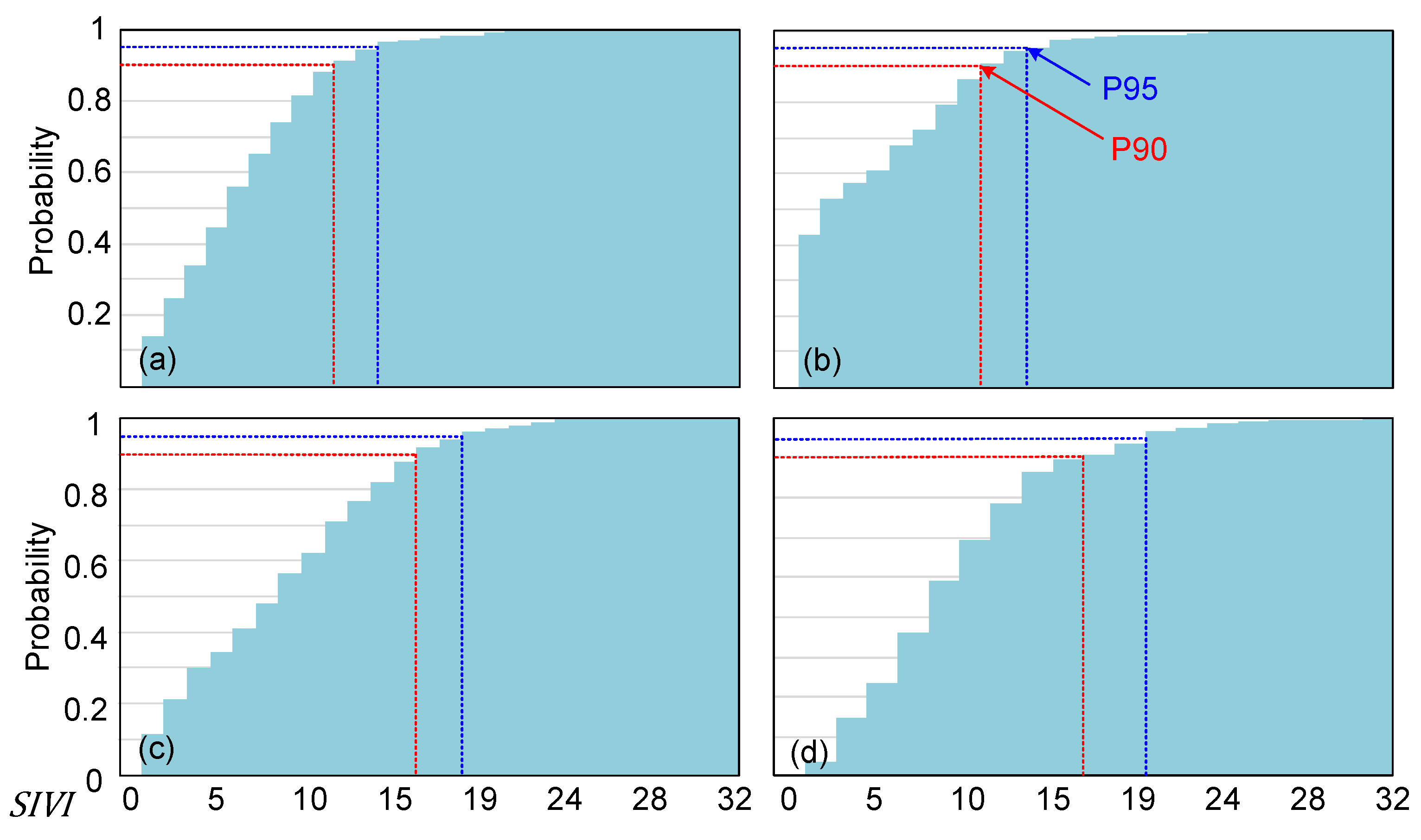
4. Performance Evaluation
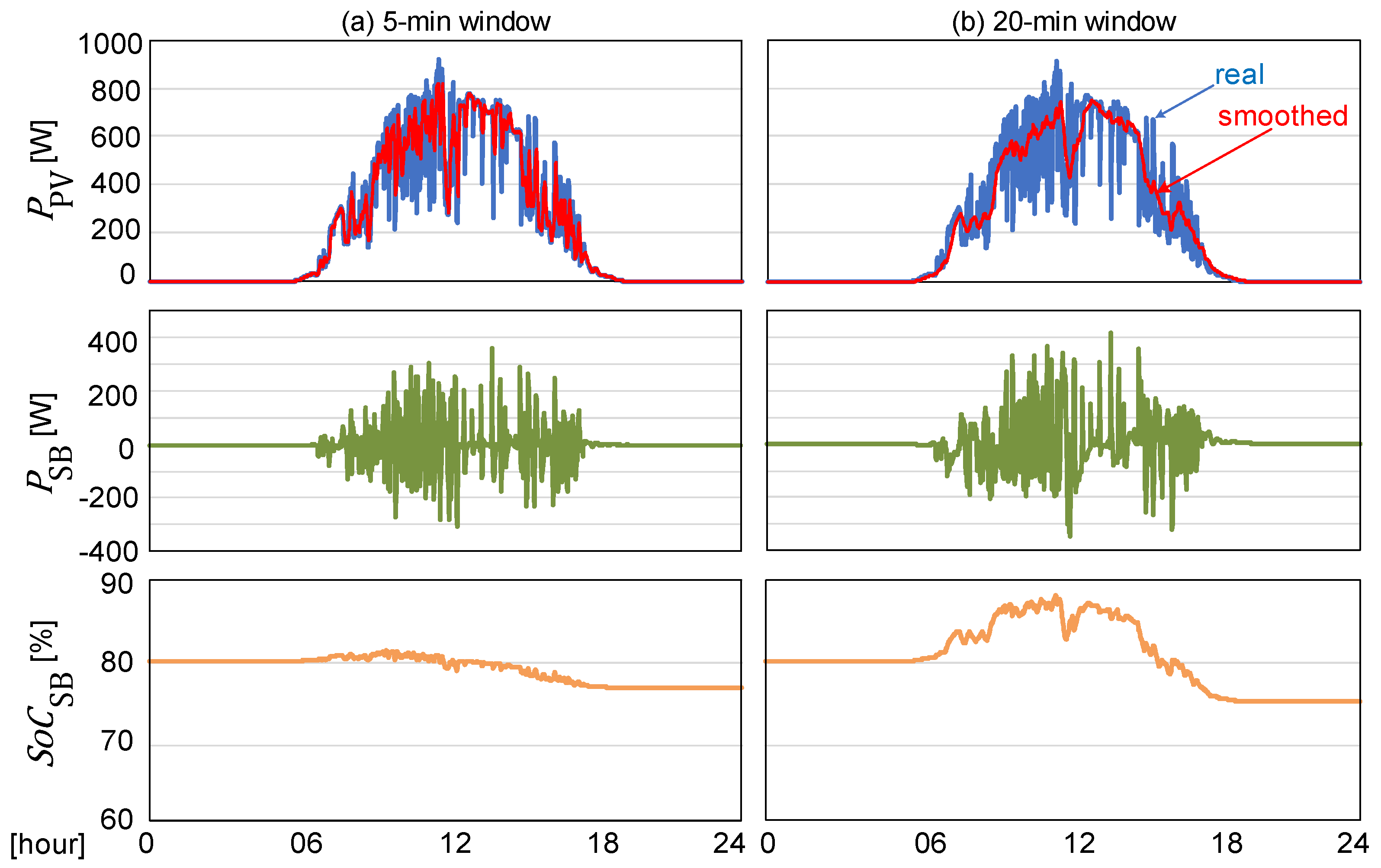
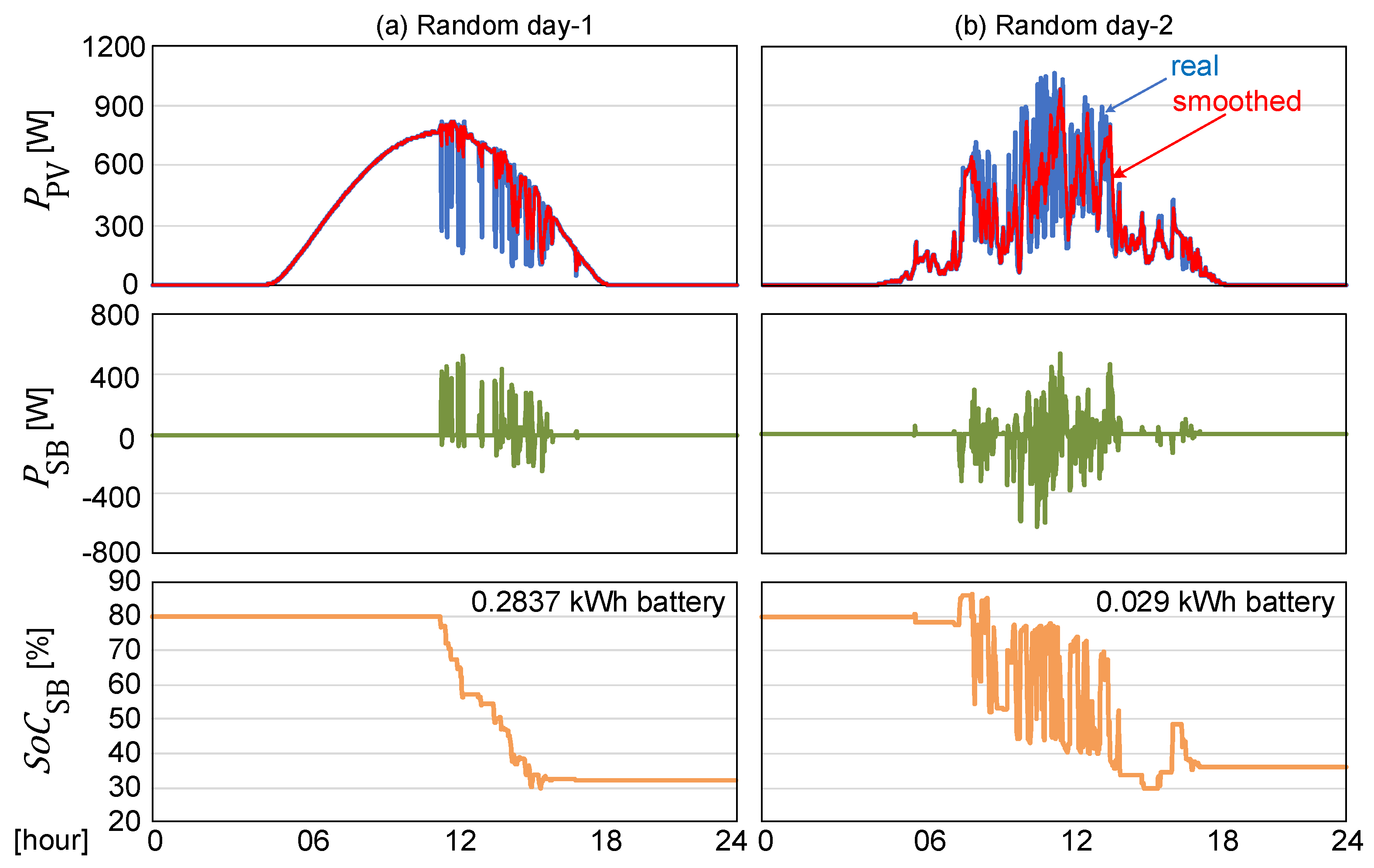
4.1. Single-Day Study Results
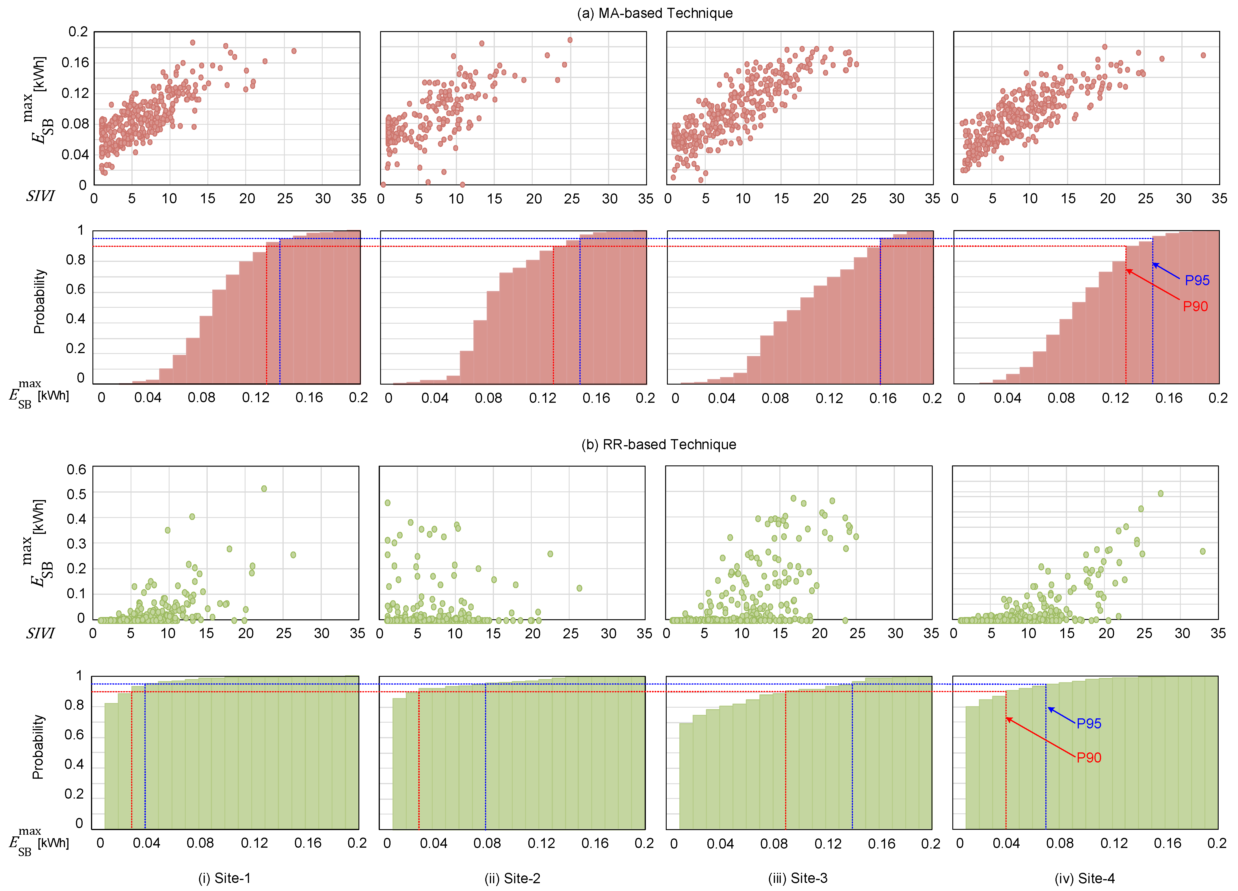
4.2. SB Selection Results
5. Comparative Analysis
6. Sensitivity Analysis
6.1. Window Size of the MA Technique
6.2. Limit of the RR Technique
6.3. SB’s Maximum Allowed DoD
6.4. SB’s Initial SoC
7. Practical Considerations and Limitations
8. Conclusions
Author Contributions
Funding
Data Availability Statement
Conflicts of Interest
Nomenclature
| 1. Abbreviations | |
| CDF | Cumulative distribution function |
| DoD | Depth of discharge |
| GHI | Global horizontal irradiance |
| MA | Moving average |
| PONE | Probability of non-exceedance |
| PV | Photovoltaic |
| RR | Ramp rate |
| SB | Smoothing battery |
| SBOC | Smoothing battery’s optimal capacity |
| SIVI | Solar irradiance variability index |
| SoC | State of charge |
| 2. Parameters and Variables | |
| SB’s nominal capacity | |
| SB’s nominal capacity defined by linear regression | |
| RR limit | |
| MA window size | |
| Smoothed output using MA technique | |
| Raw (unsmoothed) output from PV system | |
| Smoothed output using RR control technique | |
| SB’s net output under the MA control technique | |
| SB’s net output under the RR control technique | |
| Approximate SBOC | |
| Maximum allowable change in PV output in a time step (based on RR control limit) | |
| Averaging interval for SIVI calculation | |
Appendix A. Chronological Simulation Method
Appendix A.1. SB Section for a Single-Day
- (a)
- Retrieving the solar irradiance for the time step from the available dataset;
- (b)
- Calculating the PV system’s expected output power from (A1) in Appendix B;
- (c)
- Employing the MA- or RR-based smoothing technique and calculating the SB’s charging/discharging status and level from (5) or (6);
- (d)
- Calculating the smoothed output power of the PV system considering the SB’s influence;
- (e)
- Updating the SB’s SoC from the Kinetic battery model described in (A2) and (A3) in Appendix B;
- (f)
- Applying the SB’s empty or full status (based on ) to update its charging/discharging level, if required.
Appendix A.2. SBOC Selection
- (a)
- Collecting 1-min (or higher) resolution solar irradiance data for the site over at least one year;
- (b)
- Running the single-day SB selection for each day in the dataset;
- (c)
- Calculating the empirical CDFs and PONE levels for the dataset;
- (d)
- Selecting a smoothing level based on the PONE of the results and calculating the SBOC according to selected smoothing level.
Appendix B. Modeling of PV and SB Systems
Appendix C. Technical Parameters

| Parameter | Symbol | Value | Remarks |
|---|---|---|---|
| PV nominal rating | 1000 [Wp] | ||
| Environmental derating factor | 90 [%] | Assuming light to moderate soiling and dust | |
| Manufacturer output tolerance | 95 [%] | AS/NZS 4509.2 Recommendation [40] | |
| Power-temperature coefficient | 0.38 [%] | Datasheet value for a crystalline silicon module from a Tier-1 manufacturer [44] | |
| Inverter efficiency | 95 [%] | Average value for a grid-tied PV inverter from a Tier-1 manufacturer [45] |
| Discharge time (hours) | 1 | 3 | 5 | 8 | 10 |
| Discharge current (A) | 242.4 | 115.7 | 79.8 | 55.23 | 47.01 |
References
- Nayar, C. Innovative remote micro-grid systems. Int. J. Environ. Sustain. 2012, 1, 53–65. [Google Scholar] [CrossRef]
- Lazard’s Levelized Cost of Energy Analysis, Version 11.0; 2017; pp. 1–21. Available online: https://www.philipwarburg.com/wp-content/uploads/attachments/lazard-levelized-cost-of-energy-version-110.pdf (accessed on 1 July 2023).
- Susanto, J.; Shahnia, F.; Ludwig, D. A framework to technically evaluate integration of utility-scale photovoltaic plants to weak distribution systems. Appl. Energy 2018, 231, 207–221. [Google Scholar] [CrossRef]
- Somayajula, D.; Crow, M.L. An integrated active power filter-ultracapacitor design to provide intermittency smoothing and reactive power support to the distribution grid. IEEE Trans. Sustain. Energy 2014, 5, 1116–1125. [Google Scholar] [CrossRef]
- Wang, G.; Ciobotaru, M.; Agelidis, V.G. Power smoothing of large solar PV plant using hybrid energy storage. IEEE Trans. Sustain. Energy 2014, 5, 834–842. [Google Scholar] [CrossRef]
- Teleke, S.; Baran, M.E.; Bhattacharya, S.; Huang, A.Q. Rule-based control of battery energy storage for dispatching intermittent renewable sources. IEEE Trans. Sustain. Energy 2010, 1, 117–124. [Google Scholar] [CrossRef]
- Datta, M.; Senjyu, T.; Yona, A.; Funabashi, T. Photovoltaic output power fluctuations smoothing by selecting optimal capacity of battery for a photovoltaic-diesel hybrid system. Electr. Power Compon. Syst. 2011, 39, 621–644. [Google Scholar] [CrossRef]
- Wang, D.; Ge, S.; Jia, H.; Wang, C.; Zhou, Y.; Lu, N.; Kong, X. A demand response and battery storage coordination algorithm for providing microgrid tie-line smoothing services. IEEE Trans. Sustain. Energy 2014, 5, 476–486. [Google Scholar] [CrossRef]
- Khodabakhsh, R.; Sirouspour, S. Optimal control of energy storage in a microgrid by minimizing conditional value-at-risk. IEEE Trans. Sustain. Energy 2016, 7, 1264–1273. [Google Scholar] [CrossRef]
- Sun, Z.; Li, Z.; Gao, L.; Zhao, X.; Han, D.; Gan, S.; Guo, S.; Niu, L. Grafting Benzenediazonium Tetrafluoroborate onto LiNixCoyMnzO2 materials achieves subzero-temperature high-capacity lithium-ion storage via a diazonium soft-chemistry method. Adv. Energy Mater. 2018, 9, 1802946. [Google Scholar] [CrossRef]
- Sun, Z.; Li, Z.; Wu, X.L.; Zou, M.; Wang, D.; Gu, Z.; Xu, J.; Fan, Y.; Gan, S.; Han, D.; et al. A practical li-ion full cell with a high-capacity cathode and electrochemically exfoliated graphene anode: Superior electrochemical and low-temperature performance. ACS Appl. Energy Mater. 2019, 2, 486–492. [Google Scholar]
- Sun, Z.; Wu, X.L.; Xu, J.; Qu, D.; Zhao, B.; Gu, Z.; Li, W.; Liang, H.; Gao, L.; Fan, Y.; et al. Construction of bimetallic selenides encapsulated in nitrogen/sulfur co-doped hollow carbon nanospheres for high-performance sodium/potassium-ion half/full batteries. Nano Micro. Small 2020, 16, 1907670. [Google Scholar] [CrossRef]
- Senjyu, T.; Datta, M.; Yona, A.; Funabashi, T.; Kim, C.H. PV output power fluctuations smoothing and optimum capacity of energy storage system for PV power generator. Int. Conf. Renew. Energy Power Qual. (ICREPQ) 2018, 1, 35–39. [Google Scholar] [CrossRef]
- Marcos, J.; Storkël, O.; Marroyo, L.; Garcia, M.; Lorenzo, E. Storage requirements for PV power ramp-rate control. Sol. Energy 2014, 99, 28–35. [Google Scholar] [CrossRef]
- Marcos, J.; de la Parra, I.; Garcia, M.; Marroyo, L. Control strategies to smooth short-term power fluctuations in large photovoltaic plants using battery storage systems. Energies 2014, 7, 6593–6619. [Google Scholar] [CrossRef]
- Sandhu, K.; Mahesh, A. A new approach of sizing battery energy storage system for smoothing the power fluctuations of a PV/wind hybrid system. Int. J. Energy Res. 2016, 40, 1221–1234. [Google Scholar] [CrossRef]
- Mahesh, A.; Sandhu, K.; Rao, K.V. Optimal sizing of battery energy storage system for smoothing power fluctuations of a PV/wind hybrid system. Int. J. Emerg. Power Syst. 2017, 18, 20160105. [Google Scholar] [CrossRef]
- Sasmal, R.P.; Sen, S.; Chakraborty, A. Solar photovoltaic output smoothing: Using battery energy storage system. In Proceedings of the National Power System Conference, Bhubaneswar, India, 19–21 December 2016; pp. 1–5. [Google Scholar]
- Desta, A.; Courbin, P.; Sciandra, V. Gaussian-based smoothing of wind and solar power productions using batteries. Int. J. Mech. Eng. Robot. Res. 2017, 6, 154–159. [Google Scholar] [CrossRef]
- Nazaripouya, H.; Chu, C.C.; Pota, H.R.; Dagh, R. Battery energy storage system control for intermittency smoothing using optimized two-stage filter. IEEE Trans. Sustain. Energy 2018, 9, 664–675. [Google Scholar] [CrossRef]
- Li, X.; Hui, D.; Lai, X. Battery energy storage station-based smoothing control of photovoltaic and wind power generation fluctuations. IEEE Trans. Sustain. Energy 2013, 4, 464–473. [Google Scholar] [CrossRef]
- Meng, J.; Luo, G.; Ricco, M.; Swierczynski, M.; Stroe, D.I.; Teodorescu, R. Overview of Lithium-ion battery modeling methods for state-of-charge estimation. Appl. Sci. 2018, 8, 659. [Google Scholar] [CrossRef]
- Song, M.; Gao, C.; Shahidehpour, M.; Li, Z.; Lu, S.; Lin, G. Multi-time-scale modeling and parameter estimation of TCLs for smoothing out wind power generation variability. IEEE Trans. Sustain. Energy 2019, 10, 105–118. [Google Scholar] [CrossRef]
- Zhang, F.; Wang, G.; Meng, K.; Zhao, J.; Xu, Z.; Dong, Z.Y.; Liang, J. Improved cycle control and sizing scheme for wind energy storage system based on multiobjective optimization. IEEE Trans. Sustain. Energy 2017, 8, 966–977. [Google Scholar] [CrossRef]
- Zhou, Y.; Yan, Z.; Li, N. A novel state of charge feedback strategy in wind power smoothing based on short-term forecast and scenario analysis. IEEE Trans. Sustain. Energy 2017, 8, 870–879. [Google Scholar] [CrossRef]
- Zhang, F.; Meng, K.; Xu, Z.; Dong, Z.; Zhang, L.; Wan, C.; Liang, J. Battery ESS planning for wind smoothing via variable-interval reference modulation and self-adaptive SOC control strategy. IEEE Trans. Sustain. Energy 2017, 8, 695–707. [Google Scholar] [CrossRef]
- Savkin, A.V.; Khalid, M.; Agelidis, V.G. A constrained monotonic charging/discharging strategy for optimal capacity of battery energy storage supporting wind farms. IEEE Trans. Sustain. Energy 2016, 7, 1224–1231. [Google Scholar] [CrossRef]
- Brekken, T.K.; Yokochi, A.; Von Jouanne, A.; Yen, Z.Z.; Hapke, H.M.; Halamay, D.A. Optimal energy storage sizing and control for wind power applications. IEEE Trans. Sustain. Energy 2011, 2, 69–77. [Google Scholar] [CrossRef]
- Lohmann, G.M. Irradiance variability quantification and small-scale averaging in space and time: A short review. Atmosphere 2018, 9, 264. [Google Scholar] [CrossRef]
- Australian Government Bureau of Meteorology—One Minute Solar Data. Available online: http://reg.bom.gov.au/climate/reg/oneminsolar (accessed on 1 October 2018).
- Stein, J.S.; Hansen, C.W.; Reno, M.J. The variability index: A new and novel metric for quantifying irradiance and PV output variability. In Proceedings of the World Renewable Energy Forum, Denver, CO, USA, 13–17 May 2012; pp. 13–17. [Google Scholar]
- Australian Renewable Energy Agency. Hybrid power generation for Australian off-grid mines. Tech. Rep. 2018. [Google Scholar]
- Ellis, A.; Schoenwald, D.; Hawkings, D.; Willard, S. PV output smoothing with energy storage. In Proceedings of the 38th IEEE Photovoltaic Specialists Conference, Austin, TX, USA, 3–8 June 2012; pp. 1523–1528. [Google Scholar]
- Greenwood, W.; Lavrova, O.; Mammoli, A.; Cheng, F.; Willard, S. Optimization of solar PV smoothing algorithms for reduced stress on a utility-scale battery energy storage system. In Proceedings of the Electrical Energy Storage Applications and Technologies Conference, San Diego, CA, USA, 21–23 October 2013; Sandia National Laboratories: Albuquerque, NM, USA, 2013. [Google Scholar]
- Olympic Batteries DC2-500 Technical Data Sheet. Available online: https://www.olympicbatteries.com.au/wp-content/uploads/2020/09/Spec-Sheet-for-DC2-500-AusCell.pdf (accessed on 1 July 2023).
- SMA Sunny Boy Storage 3.7/5.0/6.0 Technical Data Sheet. Available online: https://files.sma.de/downloads/SBSxx-10-DS-en-31.pdf (accessed on 1 July 2023).
- Terlouw, T.; AlSkaif, T.; Bauer, C.; van Sark, W. Multi-objective optimization of energy arbitrage in community energy storage systems using different battery technologies. Appl. Energy 2019, 239, 356–372. [Google Scholar] [CrossRef]
- Marcos, J.; Marroyo, L.; Lorenzo, E.; Alvira, D.; Izco, E. Power output fluctuations in large scale PV plants: One year observations with one second resolution and a derived analytic model. Prog. Photovolt. Res. Appl. 2011, 19, 218–227. [Google Scholar] [CrossRef]
- Press, W.H.; Tuekolsky, S.A.; Vetterling, W.T.; Flannery, B.P. Numerical Recipes in C: The Art of Scientific Computing, 2nd ed.; Cambridge University Press: Cambridge, UK, 2002; pp. 397–401. [Google Scholar]
- AS/NZS 4509.2; Stand-Alone Power Systems—Part 2: System Design Guidelines. Standards Australia: Sydney, Australia, 2010.
- Manwell, J.F.; Rogers, A.; Hayman, G.; Avelar, C.T.; McGowan, J.G.; Abdulwahid, U.; Wu, K. Hybrid2: A Hybrid System Simulation Model, Theory Manual; Technical Report; National Renewable Energy Laboratory: Golden, CO, USA, 2006. [Google Scholar]
- Manwell, J.F.; McGowan, J.G.; Abdulwahid, U.; Wu, K. Improvements to the Hybrid2 battery model. In Proceedings of the American Wind Energy Association Windpower 2005 Conference, Denver, CO, USA, 15–18 May 2005. [Google Scholar]
- Manwell, J.F.; McGowan, J. Extension of the kinetic battery model for wind/hybrid power systems. In Proceedings of the 5th European Wind Energy Association Conference, Macedonia, Greece, 10–14 October 1994; pp. 284–289. [Google Scholar]
- Sunpower 225 Solar Panel Technical Data Sheet. Available online: https://www.energymatters.com.au/images/sunpower/SPR-225_com.pdf (accessed on 1 July 2023).
- SMA Tripower 5000TL–12000TL Technical Data Sheet. Available online: https://files.sma.de/downloads/STP12000TL-DEN1723-V10web.pdf (accessed on 1 July 2023).


| Refs. | High-Resolution Data | ≥1 Year of Solar Data | Multiple Locations | Battery Model |
|---|---|---|---|---|
| [7,13] | ✓ (20 s) | ✗ (1 day) | ✗ | ✗ |
| [14,15] | ✓ (5 s) | ✓ (1 year) | ✗ | ✗ |
| [16] | ✗ (1 h) | ✓ (1 year) | ✓ (two) | ✓ (Kinetic) |
| [17] | ✗ (1 h) | ✓ (1 year) | ✓ (two) | ✓ (Kinetic) |
| [18] | ✓ (1 min) | ✗ (1 day) | ✗ | ✗ |
| [19] | ✗ (1 h) | ✗ (1 day) | ✗ | ✗ |
| [20] | ✓ (30 s) | ✗ (1 day) | ✗ | ✗ |
| [21] | ✓ (≤1 min) | ✗ (1 h) | ✗ | ✓ (Internal resistance) |
| This paper | ✓ (1 min) | ✓ (1 year) | ✓ (11) | ✓ (Kinetic) |
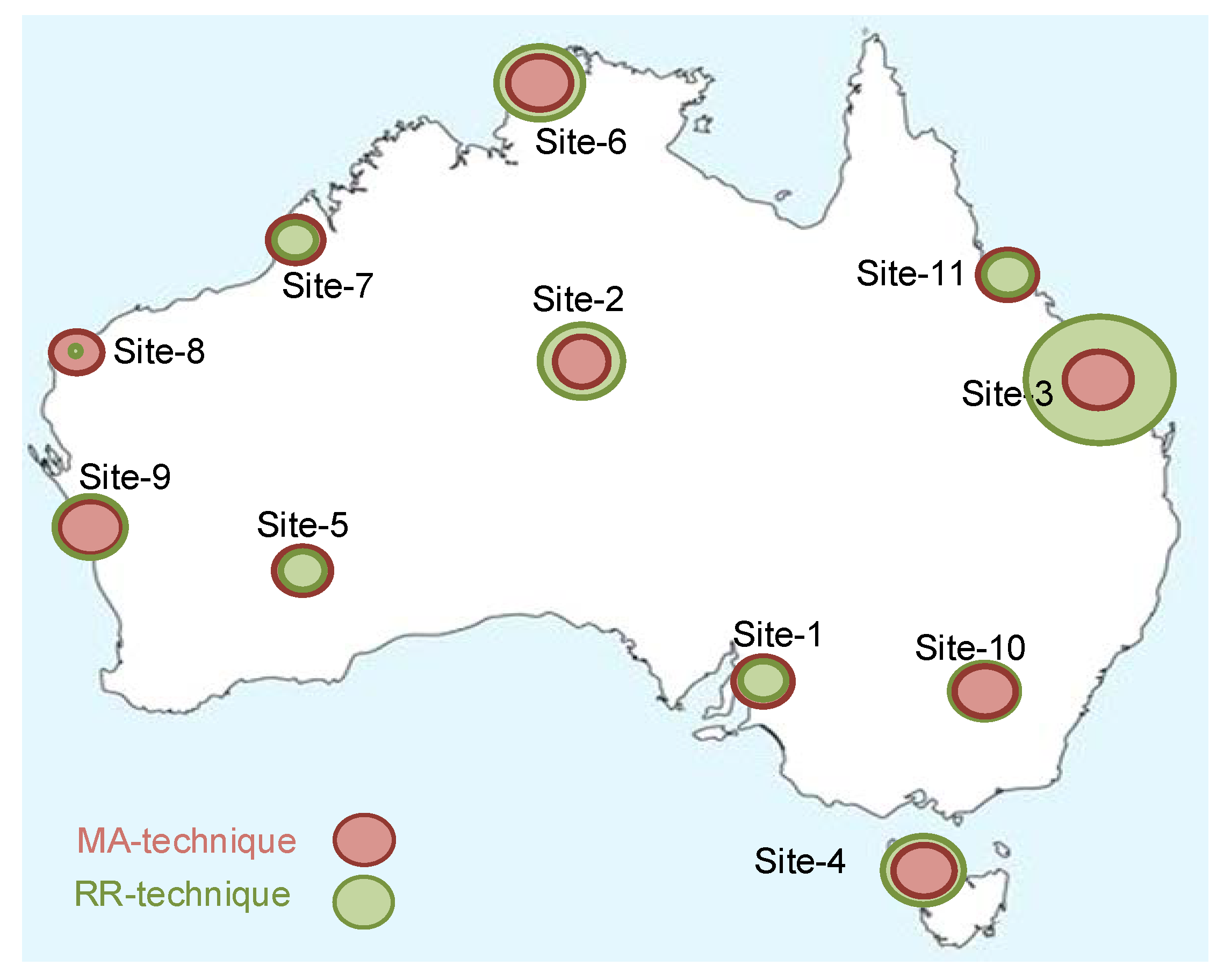
| Site | Name | State | Longitude (°) | Latitude (°) |
|---|---|---|---|---|
| 1 | Adelaide | South Australia | −34.9285 | 138.6007 |
| 2 | Alice Springs | Northern Territory | −23.6980 | 133.8807 |
| 3 | Rockhampton | Queensland | −23.3791 | 150.5100 |
| 4 | Cape Grim | Tasmania | −40.6833 | 144.6833 |
| 5 | Kalgoorlie | Western Australia | −30.7490 | 121.4660 |
| 6 | Darwin | Northern Territory | −12.4634 | 130.8456 |
| 7 | Broome | Western Australia | −17.9614 | 122.2359 |
| 8 | Learmonth | Western Australia | −22.2312 | 114.0888 |
| 9 | Geraldton | Western Australia | −28.7774 | 114.6150 |
| 10 | Wagga | New South Wales | −35.1082 | 147.3598 |
| 11 | Townsville | Queensland | −19.2590 | 146.8169 |
| PONE | Site-1 | Site-2 | Site-3 | Site-4 |
|---|---|---|---|---|
| P50 | 4.8 | 2.0 | 8.4 | 8.2 |
| P75 | 7.2 | 8.4 | 12.5 | 12.1 |
| P90 | 11.1 | 10.2 | 15.3 | 15.4 |
| P95 | 12.4 | 12.7 | 17.8 | 18.5 |
| P99 | 22.1 | 21.3 | 22.5 | 23.4 |
| P100 | 26.3 | 25.0 | 25.0 | 32.9 |
| Site | MA (10 min) | RR Limit (5%) |
|---|---|---|
| 1 | 0.7786 | 0.5633 |
| 2 | 0.7348 | 0.5750 |
| 3 | 0.8577 | 0.5966 |
| 4 | 0.8180 | 0.6981 |
| 5 | 0.7724 | 0.6914 |
| 6 | 0.7755 | 0.5629 |
| 7 | 0.7302 | 0.4431 |
| 8 | 0.8294 | 0.6383 |
| 9 | 0.7521 | 0.4469 |
| 10 | 0.7849 | 0.4334 |
| 11 | 0.8149 | 0.4621 |
| Average of all sites | 0.7862 | 0.5556 |
| Site No. | MA (10-min) | RR Limit (5%) | ||||
|---|---|---|---|---|---|---|
| Model | Detailed [kWh/kWp] | Approximate [kWh/kWp] | Deviation [%] | Detailed [kWh/kWp] | Approximate [kWh/kWp] | Deviation [%] |
| 1 | 0.140 | 0.150 | 7.1 | 0.111 | 0.149 | 34.2 |
| 2 | 0.142 | 0.152 | 7.0 | 0.212 | 0.152 | −28.3 |
| 3 | 0.159 | 0.175 | 10.1 | 0.362 | 0.188 | −48.1 |
| 4 | 0.144 | 0.179 | 24.3 | 0.198 | 0.194 | −2.0 |
| 5 | 0.136 | 0.163 | 19.9 | 0.109 | 0.168 | 54.1 |
| 6 | 0.150 | 0.167 | 11.3 | 0.214 | 0.176 | −17.8 |
| 7 | 0.130 | 0.152 | 16.9 | 0.100 | 0.151 | 51.0 |
| 8 | 0.123 | 0.140 | 13.8 | 0.019 | 0.132 | 594.7 |
| 9 | 0.151 | 0.177 | 17.2 | 0.174 | 0.192 | 10.3 |
| 10 | 0.144 | 0.165 | 14.6 | 0.166 | 0.173 | 4.2 |
| 11 | 0.140 | 0.154 | 10.0 | 0.118 | 0.155 | 31.4 |
| Technique | |||
|---|---|---|---|
| MA with 10-min window | 0.0046 | 0.0567 | 0.0315 |
| RR with 5% ramp limit | 0.0074 | −0.0221 | 0.0709 |
| SBOC Sizing Method | SBOC [kWh/kWp] | Annual Coverage [%] | |
|---|---|---|---|
| Existing Methods | Peak energy exchange | 0.131 | 92.8 |
| Hourly chronological simulation | 0.619 | 100.0 | |
| Methods of this paper | 1-min chronological simulation (P95 desired level) | 0.140 | 95.0 |
| Approximate method (P95 desired level) | 0.150 | 96.5 | |
Disclaimer/Publisher’s Note: The statements, opinions and data contained in all publications are solely those of the individual author(s) and contributor(s) and not of MDPI and/or the editor(s). MDPI and/or the editor(s) disclaim responsibility for any injury to people or property resulting from any ideas, methods, instructions or products referred to in the content. |
© 2023 by the authors. Licensee MDPI, Basel, Switzerland. This article is an open access article distributed under the terms and conditions of the Creative Commons Attribution (CC BY) license (https://creativecommons.org/licenses/by/4.0/).
Share and Cite
Susanto, J.; Shahnia, F. Optimal Capacity of a Battery Energy Storage System Based on Solar Variability Index to Smooth out Power Fluctuations in PV-Diesel Microgrids. Energies 2023, 16, 5658. https://doi.org/10.3390/en16155658
Susanto J, Shahnia F. Optimal Capacity of a Battery Energy Storage System Based on Solar Variability Index to Smooth out Power Fluctuations in PV-Diesel Microgrids. Energies. 2023; 16(15):5658. https://doi.org/10.3390/en16155658
Chicago/Turabian StyleSusanto, Julius, and Farhad Shahnia. 2023. "Optimal Capacity of a Battery Energy Storage System Based on Solar Variability Index to Smooth out Power Fluctuations in PV-Diesel Microgrids" Energies 16, no. 15: 5658. https://doi.org/10.3390/en16155658
APA StyleSusanto, J., & Shahnia, F. (2023). Optimal Capacity of a Battery Energy Storage System Based on Solar Variability Index to Smooth out Power Fluctuations in PV-Diesel Microgrids. Energies, 16(15), 5658. https://doi.org/10.3390/en16155658