Modelling and Validation of Typical PV Mini-Grids in Kenya: Experience from RESILIENT Project

Abstract

PV-based mini-grids are identified as a feasible and, often, only economically viable option for the electrification of Kenyan remote and scattered rural areas, where connection to the national grid is challenging, and the related costs are high, if not prohibitive. This paper presents the analysis of typical Kenyan PV mini-grids by using some results of the work in the project “Reliable, Efficient and Sustainable Mini-Grids for Rural Infrastructure Development in Kenya (RESILIENT)”. After presenting average annual and seasonal daily load profiles of residential and small commercial mini-grid customers identified from the measured demands, the paper introduces the main mini-grid components and their models, including a simplified, but reasonably accurate, model of a mini-grid battery storage system based on the manufacturer’s charge–discharge curves. All mini-grid components are assembled in a scalable and easily reconfigurable simulation model of an actual Kenyan PV mini-grid, and they are implemented for the evaluation of PV mini-grid performance and the potential for expansion and connection of additional residential and small commercial customers. During the validation of the developed simulation model using available measurement data, an empirical approach for adjusting the PV system output power is specified for a more accurate match with the measurements. The presented results indicate the importance of the information on the actual control algorithms and control settings of the mini-grid energy management systems, on the thermal dependencies and characteristics of both PV generation system and battery storage system, and on the availability of on-site measurements of temperature and input solar irradiance. The developed PV mini-grid model can be used for further analyses, such as to study the techno-economic performance of different mini-grid configurations, to identify the optimal sizing of mini-grid components, and to specify efficient control and operation schemes based on the locally available resources.

1. Introduction

1.1. Context and Motivation

The republic of Kenya has set ambitious targets in its long-term development plan (“Kenya Vision 2030”): to achieve universal access to electricity by 2030, as well as to ensure reliable, clean, and affordable energy for all citizens [1,2]. In recent years, despite the challenges posed by the COVID-19 pandemic, Kenya has maintained progress towards universal electricity access, which is estimated to currently be at 75% [3]. Since 2018, this effort has been underpinned by the Kenya National Electrification Strategy (KNES), which specifies a multifaceted electrification strategy of both on-grid and off-grid energy generation systems. Amongst the latter, the KNES includes stand-alone solar home systems, commonly denoted as “pico-grids”, and isolated microgrids, commonly denoted as “mini-grids” [2]. In particular, mini-grids are often identified as the only economically viable option for the electrification of remote and scattered rural areas, where connection to the national grid is challenging and the related costs are high, if not prohibitive. There is also evidence suggesting that, even in the areas that are relatively close to the national grid, mini-grids may offer quicker access and a more reliable power supply than the national grid, which frequently experiences supply interruptions and power outages, as well as long restoration times after the power outages [4].

Existing mini-grids in Kenya are predominantly based on photovoltaic (PV) generation systems, typically in combination with additional electrical (i.e., battery) energy storage. The main challenge for the economic viability of these PV-based mini-grids is the low electricity demand of households (residential load) and the small productive use of energy (PUE) customers (small commercial load). This paper presents the analysis of a typical Kenyan PV mini-grid by using some results of the work in project “Reliable, Efficient and Sustainable Mini-Grids for Rural Infrastructure Development in Kenya (RESILIENT)”. The RESILIENT project is aimed at studying existing PV-based mini-grids, with a view of improving them by incorporating multi-vector energy generation and storage in rural areas, which include a supply of thermal energy for heating, cooking, cooling and food storage, or transportation by two-wheel (2-W) and three-wheel (3-W) electric bikes and vehicles. In the context of existing PV mini-grids in Kenya, the project focuses on the replacement and avoidance of energy sources with high CO₂ emission, such as petrol and diesel for transportation and back-up power, kerosene and paraffin for lighting, liquefied petroleum gas (LPG) for cooking, etc., where significant decarbonisation can be achieved through increased utilisation of locally available renewable energy resources.

1.2. A Brief Review of Related Literature

Several studies in existing literature evaluate how the addition of PUE customers to the existing mini-grids can address a variety of challenges, including economic sustainability and the promotion of local community developments [5,6]. For example, the findings from [7] state that PUE activities can improve the utilisation of solar PV-based mini-grids, where the predominant demand from residential customers occurs during the night hours and where direct PV generation is used less than the energy stored in the dedicated battery storage system. Support for PUE activities with flexible demands will help avoid the issue of underutilized mini-grid systems due to low electricity demands, ultimately resulting in a more affordable electricity supply for mini-grid customers [8,9].

A recent review paper, [10], considers various aspects of renewable-based mini-grids in developing countries and provides a list of tools used for the optimal designing and planning of mini-grids, discussing their key features and limitations, as well as providing references to relevant studies that have employed them. The most common approaches for the optimal design of mini-grids and their techno-economic analysis are related to the use of commercial software and metaheuristic algorithms, e.g., [11,12]. It is important to note, however, that the majority of the previous work focused on planning and designing mini-grid systems, with a much lower number of references aimed specifically at the analysis and validation of existing mini-grids. Furthermore, due to a general lack of actual or prior mini-grid electricity consumption data, artificial load profiles, based on assumed electricity demands, are often used [13,14]. This highlights the importance of the findings presented in [15], where actual demand data from eight mini-grids in Kenya are compared with electricity consumption estimated from energy-use surveys, confirming that actual mini-grid demands may be overestimated up to a factor of four. The overestimated demands, then, can have significant financial implications for mini-grid developers, as they may lead to potential financial losses and result in higher electricity tariffs to recoup the investment in over-sized systems, making mini-grids less appealing to customers in low-income areas.

This paper aims to fill some of the identified gaps in the existing literature, on the modelling and validation of PV mini-grids, by utilizing data and measurements from an actual mini-grid in Kenya and presenting average annual and seasonal daily load profiles of the main types of mini-grid customers. The presented analysis is based on the work in the RESILIENT project, where three rural communities that operate mini-grids in Nyamira County, Nakuru County, and Kisii County are selected as the pilot sites for evaluating their potential for extension and the connection of new customers, as well as for the deployment of three field trials of multi-vector mini-grids, integrating electrical, thermal, transport, and other energy vectors into typical PV mini-grid systems. The PUE activities in these mini-grids include: posho mills (maize milling), hatcheries, and agricultural value chains activities, such as post-harvesting processes (cold storage, solar drying, ice making). At the time of writing this paper, the three field trials in the selected pilot rural communities are in progress, with each of them aiming to evaluate the benefits of deploying specific multi-vector energy extensions to the existing PV mini-grid:

(1)

Use of 2-W and 3-W EVs, with locally available battery charging and battery swapping stations, for transporting goods and people;

(2)

Electrical heating of water, supplemented with a solar-thermal plant and thermal energy storage system, for related PUE activities, e.g., the breeding of black soldier fly larvae as chicken feed;

(3)

Water pumping and purification plant (by reverse osmosis) in an existing PV mini-grid rural community without proximate access to a clean drinking water source.

1.3. The Main Contributions of the Paper

The main contributions of this paper are:

• Specification of typical PV-based mini-grids in Kenya and Sub-Saharan Africa, including average annual and seasonal daily load profiles of main types of customers;
• Formulation of a suitable empirical approach for evaluating variations and uncertainties in the output powers of a PV system when solar irradiance measurements at the actual PV mini-grid site are not available;
• Development and validation of a simplified, but reasonably accurate, battery storage model based on the manufacturer’s charge–discharge curves;
• Evaluation of PV mini-grid performance and the potential for expansion and connection of additional residential and PUE customers based on the use of actual field data.

The rest of this paper is structured as follows: an overview of typical solar PV-based mini-grids in Kenya is presented in Section 2; Section 3 describes the modelled mini-grid components; modelling of mini-grid loads is presented in Section 4; Section 5 discusses modelling of renewable energy resources; Section 6 provides the results of the validation of the developed mini-grid model; Section 7 discusses the potential for an extension of the considered mini-grid; conclusions and closing discussion are provided in Section 8.

2. Typical Kenyan PV-Based Mini-Grid

2.1. A Brief Overview and Some Statistical Data

Currently, Kenya has around 500 mini-grids in operation or under construction (of which, 324 are PV-based), mainly serving areas with limited access to the national grid, the majority of which are in rural villages. Due to a very good year-round availability of the solar energy resource, Kenyan mini-grids typically combine PV generation with battery energy storage, and they also have a diesel generator for a back-up power supply.

Table 1. Number of mini-grids listed by installed PV capacity in Kenya.

Installed PV Mini-Grid Capacity	Number of Sites
0 to 50 kWp	155
51 to 100 kWp	112
101 to 150 kWp	33
151 to 200 kWp	8
201 to 250 kWp	5
>251 kWp	11

. The number of mini-grids, listed by installed PV capacity, shows some statistical data extracted by the authors, for Kenyan PV mini-grids, in terms of the installed generation capacity.

2.2. Typical Mini-Grid PUE Applications

Typical PUE applications in Kenyan mini-grids for activities within the agriculture sector include: solar-powered water pumping systems for boreholes, shallow wells and surface water, solar sprayers, and farm irrigation systems. Furthermore, grain milling, drying, grinding, hulling, threshing, crushing, oil pressing, and walk-in cold rooms for the preservation of fruits and vegetables are additional agricultural PUE activities related to post-harvest handling. The main barriers and challenges encountered in the business models identified in this category are the high upfront costs of the machinery and the scarcity of spare parts. Some of the PUE cases in the dairy, poultry, and livestock sector include chillers and freezers for meat preservation, as well as cold rooms or chillers tanks for milk preservation. Egg incubators and chicken brooders are also commonly found to be mini-grid PUEs in this segment, where high upfront costs have been noted as the main challenge. Examples of PUE applications in the fishing industry include: portable rechargeable lights, battery powered boat motors, and ice-making machines.

The PUE mini-grid applications in the small to medium enterprise (SME) segment mostly represent commercial activities and businesses, such as dressmaking shops, welding and woodwork workshops, phone charging, car/solar battery charging, electronics repair shops, salons and barbershops, as well as water purification and shops/vending/retail premises.

The PUE applications in the electric mobility sector include the use of electric bikes and smaller 2-W/3-W electric vehicles as alternatives to internal combustion engines (ICEs). The primary barriers to the growth of the electric mobility market include high up-front costs associated with purchasing the vehicles, limited charging infrastructure, a scarcity of spare parts and repair expertise, tough terrain that often results in damage to the vehicles, and a general lack of supporting policies to compete with ICE alternatives.

2.3. Opportunities for Further PUE Applications in Mini-Grids

PV mini-grid developers are actively incorporating PUE activities as “demand-stimulation” approaches while, at the same time, testing different business models in order to determine which would work best for each activity. In particular, the PUEs that can sustain year-round demand will have strong beneficial impacts on mini-grid developers in terms of increased revenue, which derives from consumers’ ability to pay for electricity as they generate income from PUE. At the same time, the increased electricity demand could translate to lower electricity costs for the consumer.

In the three rural villages that were surveyed in the RESILIENT project, around 98 % of households still cultivate their crops manually. This presents an opportunity to increase crop production and productivity through the promotion of mechanized farming practices, including farm irrigation systems. Other farming opportunities include the promotion of “value addition” through the agricultural processing of cultivated crops.

Most households also struggle with the lack of nearby access to drinking water. This provides an opportunity to increase accessibility to potable, high-quality water through secure boreholes, water pumping, water treatment, and rainwater harvesting. Furthermore, the findings of the study of the three considered Kenyan rural communities indicate heavy use of firewood and kerosene for cooking, heating, and lighting. This presents a potential to reduce high smoke and CO₂ emissions through the promotion of alternative and clean sources of energy, such as biofuels and renewable-based electricity. Finally, in one of the three villages, there was a black soldier fly (BSF) facility for processing fruit waste from the local markets for fertiliser and chicken food production, for which thermal energy was required for heating and drying. This BSF plant was included in the field trials of multi-vector energy supply (electricity and thermal energy generation and storage) in one of the considered PV mini-grids with a view of evaluating benefits for a medium to large-sized PUE customer.

3. Mini-Grid Modelling

3.1. Description and Layout of the Modelled PV Mini-Grid

The mini-grid model presented in this section is based on an actual Kenyan mini-grid (Gionseri B site in Kisii County), which was selected as one of the pilot rural communities in the RESILIENT project. The Gionseri B mini-grid was commissioned in 2020 and is still operational, serving around 1875 customers and 374 households, as well as a communal/administrative building, which are all connected through single-phase metered service connections. The PV system peak output power and battery storage capacity in this mini-grid are 59.4 kWp and 142.2 kWh, respectively. The owner and operator of the Gionseri B mini-grid is Power Hive East Africa Ltd. (PH), and a pre-paid metering system is used for both residential and PUE customers, which include chicken brooders, EV charging stations, and posho mills.

Figure 1a depicts the Gionseri B mini-grid layout, which is used to develop the electrical network schematic (single-line diagram) displayed in Figure 1b. The main mini-grid model components are: the PV array, consisting of 180 polycrystalline PV panels, (each rated at 330 Wp); a pack of LiFePo batteries for energy storage, rated at 162 kWh; a three-phase DC-AC inverter, rated at 50 kW; a 315 V/400 V transformer with 50 kVA power. In cases when PV generation and battery storage, together, cannot supply the mini-grid load, or in case of an emergency, the Gionseri B mini-grid has a 12 kW back-up diesel generator. Key assumptions for the developed mini-grid model include:

• While the general structure of the mini-grid and its components is known, the actual circuit designs and controls of each part/component (e.g., battery charger or inverter controllers) are taken from available manufacturer specifications or assumed as the typical ones when this information was not available.
• A “Perturb & Observe” algorithm was used to model maximum power point tracking (MPPT) control.
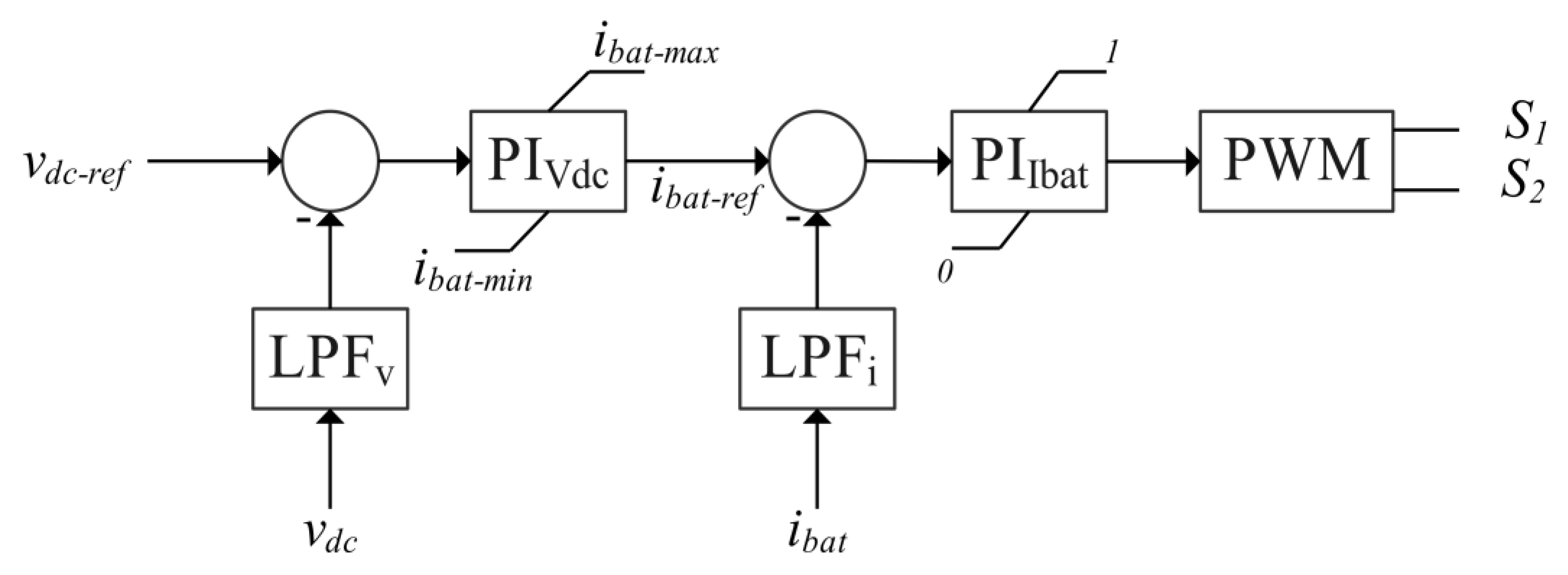
• Proportional integral (PI) controllers are assumed to be the main controller type for battery and inverter, for which parameters are fitted using available measurement data, i.e., they are not designed through the control system design process.

The following subsections describe, in more detail, the modelled mini-grid components and controls that are developed using modelling software from [16].

3.2. Mini-Grid Model Components

3.2.1. PV Panels

The modelled PV array, with total peak power output of 59.4 kWp, consists of a number of interconnected individual PV modules from [17]: 10 parallel strings, each with 18 series-connected modules. Electrical characteristics of the PV panels are listed in

Table 2. Electrical characteristics of modelled PV panel from [17].

Description	Value
Cell Type	Polycrystalline, 6-inch
Nominal Maximum Power	330 W
Voltage at Maximum Power Point	37.2 V
Current at Maximum Power Point	8.88 A
Open Circuit Voltage	45.6 V
Open Circuit Current	9.45 A
Module Efficiency	16.97%
Operating Temperature	−40 °C~+85 °C

and illustrated in Figure 2, comparing data from the manufacturer’s specification with the results of simulation. The PV array simulation model is developed in [16] using [17,18], which incorporates both user-settable and pre-defined PV modules, including the one from [17]. The I–V curves for different solar irradiance levels and ambient temperatures in Figure 2 show that the simulation model (dash-dot lines) closely matches manufacturer data (solid lines).

3.2.2. Energy Storage System–-Lithium-Iron Phosphate (LiFePo) Battery Pack

The daily surplus PV power output (i.e., exceeding the demand of the mini-grid loads) is used for charging the battery storage units for later use, typically during the night hours or when solar irradiance levels are low (early morning, late afternoon, and evening or due to a dense cloud coverage during the day). Although the total battery storage capacity is 162 kWh, only 146 kWh are utilised, as the minimum state of charge (SoC), below which discharging is prevented to maximise the battery lifetime, is set to 20%. The LiFePo battery pack consists of two parallel strings, each with 10 series-connected battery modules from [19].

Table 3. Characteristics of the modelled battery module from [19].

Description	Value (Single Module)	Value (Battery Pack)
Battery Type	LFP (LiFePO4)
Battery Model	M38210-S
Operating Temperature Range	−10 °C~+50 °C
Depth of Discharge (DoD)	90%
Cycle Life	≥6000
Nominal Voltage	38.4 V	384
Internal Resistance	≤10 mΩ	≤250 mΩ
Operating Voltage Range	36~43 V	360~430 V
Energy Capacity	8.1 kWh	162 kWh
Usable Capacity	7.3 kWh	146 kWh
Maximum Charge Current	105 A (0.5 C)	210 A
Maximum Discharge Current	105 A (0.5 C)	210 A

lists characteristics of the modelled battery module.

Equivalent Battery Model Based on Charge–Discharge Curves

The component libraries from [20] contain a pre-built battery model/block that implements a generic dynamic model that represents the most common types of rechargeable batteries (i.e., Lithium–Ion, Lead–Acid, Nickel–Cadmium, and Nickel–Metal–Hydride). However, this battery model was impractical for evaluating mini-grid performance due to the computational complexity and long simulation times. Accordingly, this paper presents an alternative simplified approach for modelling battery storage, based on the available manufacturer charge–discharge curves. This model is simple yet reasonably accurate, enabling, for example, the simulation of daily (24 h) values in a much shorter time, while correctly modelling the key battery characteristics—particularly, variations of SoC values—due to the charging and discharging, e.g., following daily generation profiles of PV plants and daily load profiles of demands (both are modelled with a 1 h step).

The steady-state value of battery voltage will vary based on the battery SoC and the rate of charging or discharging in the actual operating conditions. A Thévenin equivalent circuit, as shown in Figure 3, consisting of a voltage source connected in series with a variable SoC-dependent resistor, is used to represent a simplified battery model in steady state. The SoC, which is the ratio of energy storage in the battery at a given time to the rated energy storage capacity of the battery, will determine the V_OC. The relationship between SoC and $V_{OC}$ can be calculated from the charge–discharge curves in the manufacturer’s specification shown in Figure 4. At one specific SoC value, five $V_{bat}$ values can be observed depending on the corresponding current-curve. Using the linear fitting, the value of $V_{oc}$ and $R_{bat}$ can be calculated for all SoC points from Equation (1), giving the relationship between $V_{OC}$ and SoC.

The specific current flowing for a period of time into/out of the battery will cause the change in the energy stored (SoC), based on the corresponding charge–discharge curves provided by the manufacturer [10]. The change of the energy stored in the battery will then change the battery open circuit voltage, $V_{OC}$, which is dependent only on the SoC in the model. Flow of the current through R_bat will also result in a voltage drop, which then determines the new battery voltage. The model can replicate steady-state battery voltage values, due to the changes of SoC caused by charge–discharge current, as expressed in Equation (1).

$$\begin{array}{cc}{V}_{bat}=V_{oc}-I_{bat} R_{bat};& \begin{array}{cc}{I}_{bat}>0& discharging\\ I_{bat}<0& charging\end{array}\end{array}$$

(1)

where: $V_{bat}$ is the terminal battery voltage; $I_{bat}$ is the discharging–charging current; $V_{oc}$ is the internal open circuit voltage, and $R_{bat}$ is the internal SoC-dependent series resistance. A positive value of $I_{bat}$ denotes the discharging of the battery, while a negative value denotes charging. The terminal voltage $V_{bat}$ is higher than $V_{oc}$ when the battery is charging, but lower when discharging, due to the voltage drop across the series resistance $R_{bat}$. The simulation model is built with battery voltage $V_{bat}$ as the model output and battery current $I_{bat}$ as the input.

For a given/constant ambient temperature, the battery charge–discharge characteristics are given in the manufacturer’s datasheet [21], which also provides data on the changes in V_bat at different temperatures. The total capacity of the battery cell changes with the increase in the battery temperature, but that change is small: the change of the battery temperature from rated temperature (25 °C) to 55 °C will impact the change of the battery voltage by only 0.2%. Therefore, in the presented model of the battery, the effect of the temperature is not considered.

For a general representation, the discharge capacity, $C_{dis}$, given by the manufacturer datasheet [21], as given in Figure 4a, can be converted using Equation (2) into the SoC, as shown in Figure 4b, which is the usual way to represent the battery capacity.

$$SoC=\frac{C_{rated}-C_{dis} }{C_{rated}}\times 100$$

(2)

where $C_{rated}$ is the rated capacity of the battery pack, $C_{dis}$ is the discharged capacity resulting due to the flow of the current, and SoC is the state of charge in percentage.

Model of the Battery Pack

Operating points at different SoC with different discharging currents can be used to obtain relationships for open circuit voltage ($V_{oc}$) and series resistance ($R_{bat}$) as functions of battery SoC, e.g., in the form of a look-up table. In Figure 5, polynomial fitting is used as a suitable way to accurately represent changes of the $V_{oc}$ (fifth order polynomial, Equation (1)) and $R_{bat}$ (fourth order polynomial, Equation (2)) for a single cell, where the highest R² value among the tried polynomial fits is selected for modelling.

$$\begin{array}{cc}{V}_{oc}=& 13.56{\left(SoC\right)}^5-34.93{\left(SoC\right)}^4+33.03{\left(SoC\right)}^3\\ & -14.06{\left(SoC\right)}^2+2.77\left(SoC\right)+3.00\end{array}$$

(3)

$$\begin{array}{cc}{R}_{bat}=& 12.39{\left(SoC\right)}^4-25.53{\left(SoC\right)}^3+\\ & 18.68{\left(SoC\right)}^2-5.68\left(SoC\right)+1.32\end{array}$$

(4)

where $V_{oc}$ is cell voltage in Volts; SoC is the per-unit state of charge varying from 0 (completely discharged battery) to 1 (fully charged battery), $R_{bat}$ is the internal series resistance of the battery in mΩ, and all constants are given with two decimal points in all fittings.

The open circuit voltage of a whole battery pack is obtained by multiplying the nominal single-cell voltage (3.2 V) by the number of series-connected cells in a module (i.e., 12 cells) and, then, by the number of series-connected modules in a pack (i.e., 10 modules), which equals the total nominal battery voltage of 384 V. Similarly, the nominal capacity of the battery pack is obtained by multiplying the single-cell capacity of 105 Ah (1 C for 1 cell, i.e., the rated/maximum charging or discharging current for 1 cell, is 0.5 C or 105 A) by the number of parallel connected cells in a module (i.e., 2) and the number of modules in the battery pack (i.e., 2), which equals a total nominal battery capacity of 420 Ah. As mentioned, the battery is controlled to not be discharged below 20 % of SoC, so the usable capacity of the whole battery pack will be 336 Ah or 129 kWh. The open circuit voltage of the battery pack can be calculated using Equation (5), while the series resistance can be calculated using Equation (6).

$$V_{oc-pack}=V_{oc-cell}\times N_{sm}\times N_{sp}$$

(5)

$$R_{bat-pack}=R_{bat-cell}\times \frac{N_{sm}}{N_{pm}}\times \frac{N_{sp}}{N_{pp}}$$

(6)

where $V_{oc-pack}$ is the open circuit voltage for a whole battery pack; $R_{bat-pack}$ is the equivalent internal series resistance of the whole battery pack; $V_{oc-cell}$ is the open circuit voltage of a battery cell; $R_{bat-cell}$ is the internal series resistance of a battery cell; $N_{sm}$ is the number of the series-connected cells in a module; $N_{pm}$ is the number of the parallel connected battery cell in a module; $N_{sp}$ is the number of series-connected modules in the pack, and the $N_{pp}$ is the number of parallel connected battery modules in the pack.

Figure 6 shows the circuit model of the battery pack, where the output is $V_{OC}$, as determined by the SoC level. The integral block calculates the change in SoC, as shown in Equation (7), from the initial SoC, SoC_in value, which is also an input in the integral block.

$$SoC=\frac{-\int i_{bat}\left(t\right) dt}{Capacity \left(As\right)}+So{C}_{in}$$

(7)

3.2.3. Power Electronic Converters

The modelled mini-grid has both DC and AC buses, as illustrated in Figure 1, where a central inverter rated at 50 kW is utilised to convert DC power, from either the PV system or battery storage to AC power, to supply electricity to the mini-grid AC loads. Both the solar PV array and battery are connected to the same DC–AC inverter, which also has a Maximum Power Point Tracking (MPPT) control, shown as a separate DC–DC converter block in Figure 1. Finally, a bidirectional DC–DC boost converter is installed for the charging and discharging of battery energy storage system.

In the developed model, three separate converters are designed to correctly represent the actual operation of the mini-grid, all of which are described in the next sub-sections.

DC-DC Boost Converter for PV Array Power

A DC–DC boost converter is modelled for the connection of the PV panels to the common DC bus, as shown in Figure 7. As the voltage output of the PV panel is not constant, but it varies with the input solar irradiance and temperature, the boost converter is controlled to extract the maximum power from the PV array, where the duty cycle is set by the MPPT control and Pulse Width Modulation (PWM) technique that regulates the operation of the converter’s power electronic switch. $L_{pv}$ and $C_{pv}$ comprise the input filter connected at the PV terminals. $S_{pv}$ represents the status of the power electronic device (MOSFET or IGBT), and D represents diode. $C_{dc}$ is the capacitor connected at the terminals of the common DC bus. While designing the boost converter, the $C_{dc}$ will be the sum of the all the capacitors connected at the DC bus terminal.

The controller schematic for the boost converter is shown in Figure 8. The PV boost converter operates in two modes. In Mode 1, when the state of charge SoC is below 99.9%, the converter functions in MPPT mode, and the PV boost converter is controlled to achieve MPPT by regulating the voltage at the PV input terminal to the optimal power point during normal operation. When the power generated by the PV array exceeds the load demand, the battery will charge until it reaches $So{C}_{max}$ (99.9 %). Once this occurs, the controller switches to Mode 2 (curtailment mode), where it maintains a constant DC voltage to ensure that the power output of the PV system matches the power required by the load. At this point, the battery will no longer charge, and the power output of the PV system must be curtailed.

$$d=\left\{\begin{array}{cc}MPPT\left(v_{pv},i_{pv}\right)& SoC\le 99.9\%\\ P{I}_{Ipv}\left(i_{pv-ref}-LP{F}_i·i_{pv}\right)& SoC>99.9\%\end{array}\right.$$

(8)

$$i_{pv-ref}=P{I}_{Vdc}\left(v_{dc-ref}-LP{F}_v·v_{dc}\right)$$

(9)

The controller’s two modes of operation are specified by Equations (8) and (9), where $v_{pv}$ and $i_{pv}$ are the voltage and current output of the PV system fed-in to MPPT and where output of the MPPT is the duty cycle required to operate the boost converter at MPP. $v_{dc-ref}$ is the DC bus voltage reference, $v_{dc}$ is the feedback voltage of the DC bus, and their difference is fed into PI controller ($P{I}_{Vdc}$) to set the reference ($i_{pv-ref}$) for the current control loop. A low pass filter ($LP{F}_v$) is used for the feedback voltage to remove high frequency variation in the voltage due to switching. The difference of the feedback current ($i_{pv}$) and the reference current is inputted into another PI controller $\left(P{I}_{Ipv}\right)$, which sets the required duty cycle to operate the PV boost converter in curtailment mode. Another low-pass filter ($LP{F}_i$) is used for the feedback current. The $i_{pv\_ref}$ has the upper limit of maximum current that could be supplied by the PV system and a lower limit of 0, since power can flow only in one direction. The upper limit for the duty cycle is set to 1, while the lower limit is 0. The switch $S_{pv}$ is derived with this duty cycle by a PWM technique.

The “Perturb & Observe” (P&O) MPPT algorithm is used in the mini-grid model, presented in Figure 9, due to its simplicity. It is implemented on the PV-side of the DC–DC boost converter to vary the duty cycle in order to generate the required voltage reference for the boost converter and extract the maximum power output for all operating conditions.

DC-DC Boost Converter for Battery Control

Figure 10 displays the battery-side bi-directional DC–DC boost converter that is modelled to control the battery storage system, while its charge controller is shown in Figure 11. The battery controller is modelled as a simple two-stage PI, controlled to track a current reference, which keeps the DC bus voltage at the specified value. Increased DC bus voltage indicates that the power from the PV is greater than the power utilized by the load, which will result in a negative current reference, indicating the battery charging status. If the power from the PV system is below the power demanded by the load, the DC bus voltage will begin to drop, triggering the discharging of the battery.

$$d=P{I}_{Ibat}\left(i_{bat-ref}-LP{F}_i·i_{bat}\right)$$

(10)

$$i_{bat-ref}=P{I}_{Vdc}\left(v_{dc-ref}-LP{F}_v·v_{dc}\right)$$

(11)

The battery controller equations are outlined in Equations (10) and (11), where $V_{dc-ref}$ is the reference DC voltage, and $v_{dc}$ is the feedback DC bus voltage inputted through a low pass filter ($LP{F}_v$). A PI controller ($P{I}_{Vdc}$) is used to set the reference current for the current control loop. The upper limit of reference current is maximum allowed discharging current (a positive value), while the lower limit is the maximum allowed charging current (a negative value). Another PI controller ($P{I}_{Ibat}$) is used for the current control loop. The error signal is generated by comparing reference current ($i_{bat-ref}$) and feedback current ($i_{bat}$) after passing through a low pass filter to remove high frequency components. The output of the $P{I}_{Ibat}$ will be the duty cycle required to drive the bidirectional DC–DC converter. $S_1$ and $S_2$ are the power electronic switches, which are operated in complimentary fashion with the help of PWM.

DC-AC Inverter

The mini-grid inverter is supplying a mixture of single-phase and three-phase loads via a four-wire, three-phase distribution network. A neutral conductor is often needed to provide a current path for the unbalanced loads or when different phases of an inverter need to be independently operated (so that the coupling effects among the phases are minimised). Accordingly, the modelled inverter is supplemented with a neutral conductor connecting to the mini-grid distribution network, i.e., the actual mini-grid inverter is modelled as a three-phase, four-wire inverter with split DC link capacitors, as shown in Figure 12.

Figure 13 illustrates the PI-based control scheme implemented in dq-frame (on both the d and q-axis) to control the output voltage and current of the inverter, where the reference output currents in dq-frame, $I_{d-ref}$ and $I_{q-ref}$, are generated to stabilize the output AC voltage. If the reference current is constant, the inverter is controlled as a constant current source ($P_{load}=P_{pv}-P_{bat}$). The reference voltage for the d-axis is the peak value of the inverter output line voltage ($V_{d-ref}=315$ V), while the reference voltage for the q-axis is zero ($V_{q-ref}=0$).

$$\begin{gathered} d_d=P{I}_{Iac}\left(I_{d-ref}-i_d\right)-{\omega }_0{L}_f{i}_q \\ {d}_q=P{I}_{Iac}\left(I_{q-ref}-i_q\right)-{\omega }_0{L}_f{i}_d \end{gathered}$$

(12)

$$\begin{gathered} I_{d-ref}=P{I}_{Vac}\left(V_{d-ref}-v_{Cd}\right)+i_{Ld}-{\omega }_0{C}_f{v}_{Cq} \\ {I}_{q-ref}=P{I}_{Vac}\left(V_{q-ref}-v_{Cq}\right)+i_{Lq}-{\omega }_0{C}_f{v}_{Cd} \end{gathered}$$

(13)

Equations given in (12) and (13) describe the inverter controller, where $d_d$ and $d_q$ are the duty cycle used to drive the inverter in dq-frame, respectively; $i_d$ and $i_q$ are the feedback currents in dq-frame; $L_f$ is the filter inductance; ${\omega }_0$ is the grid frequency in rad/s; $I_{d-ref}$ and $I_{q-ref}$ are the reference currents in dq-frame; $v_{Cd}$ and $v_{Cq}$ are the feedback voltages across the filter capacitor; $i_{Ld}$ and $i_{Lq}$ are the currents flowing through the filter inductor; $V_{d-ref}$ and $V_{q-ref}$ are the reference AC voltages in dq-frame. $P{I}_{Iac}$ and $P{I}_{Vdc}$ are the PI controllers for the current and voltage control loops, respectively.

3.2.4. Low-Pass Output Filter

To meet power quality requirements in terms of the sinusoidal AC voltage waveform supplying the mini-grid loads, a low-pass filter is necessary to filter out harmonics due to the inverter PWM switching operation (and connected non-linear loads). Figure 14 shows the schematics of the designed LC-type filter. The resonant frequency is calculated using Equation (14), while the inductor and capacitor values in the LC-type filter can be calculated using Equations (15) and (16).

$$f_0=\frac{1}{2\pi }\frac{1}{\sqrt{LC}}$$

(14)

$$C_{fmax}\le \frac{0.05\times P}{2\pi ·f·V^2}$$

(15)

$$L_{fmax}\le \frac{0.1\times V^2}{2\pi ·f·P}$$

(16)

where $C_{fmax}$ and $L_{fmax}$ are the maximum limits for the filter capacitor and inductor; $P$ is the rated power of the inverter, and $V$ is the rated RMS voltage. Once the maximum values are calculated, any combination of inductor and capacitor values can be used until $f_0\gg f_s$, where $f_0$ is the resonance frequency of the filter, and $f_s$ is the AC supply system frequency.

Table 4. The LC filter elements.

Description	Value
Cfmax	80.2 µC
Lfmax	1.1 mH
Lf	1.1 mH
RLf	0.1096 Ω
Cf	46.206 µC
RCf	1 µΩ
f0	706 Hz

lists the values used for the modelled low-pass LC filter.

3.2.5. Three-Phase Transformer

A 50 kVA, 315 V/400 V three-phase transformer is installed in the modelled mini-grid, serving as both an isolation transformer between the inverter and the load side and as a voltage regulation component. The transformer adds leakage inductance on the load-side (inductor $Lg$ in Figure 14b), forming an LCL-type filter with the corresponding component values listed in

Table 5. The LCL filter elements.

Description	Value
Lf	1.1 mH
RLf	0.1096 Ω
Cf	46.206 µC
RCf	1 µΩ
Ltran	0.5053 mH (0.08 pu)
Rtran	1.9845 mΩ (0.001 pu)
f0	1250 Hz

. The resonant frequency of the LCL filter can be calculated as shown in Equation (17).

$$f_0=\frac{1}{2\pi }\sqrt{\frac{L_f+L_g}{L_f{L}_g{C}_f}}$$

(17)

3.2.6. Distribution Network (Overhead Lines and Cables)

In the modelled mini-grid, the power distribution network was made of 400 V three-phase power lines spread to an average radius of 1 km (the farthest pole to the PV generation plant, positioned in the centre of the mini-grid, is at a distance of around 1.6 km). Figure 15 shows a map representation of the modelled mini-grid, indicating the general layout and geographical spread of the mini-grid distribution network (the names of the actual locations on the map are neither needed nor relevant for the presented analysis). All distribution lines are modelled as a simple series RL branch, for which values are taken from the manufacturer datasheet in [22].

4. Mini-Grid Load Modelling and Demand Time-Series

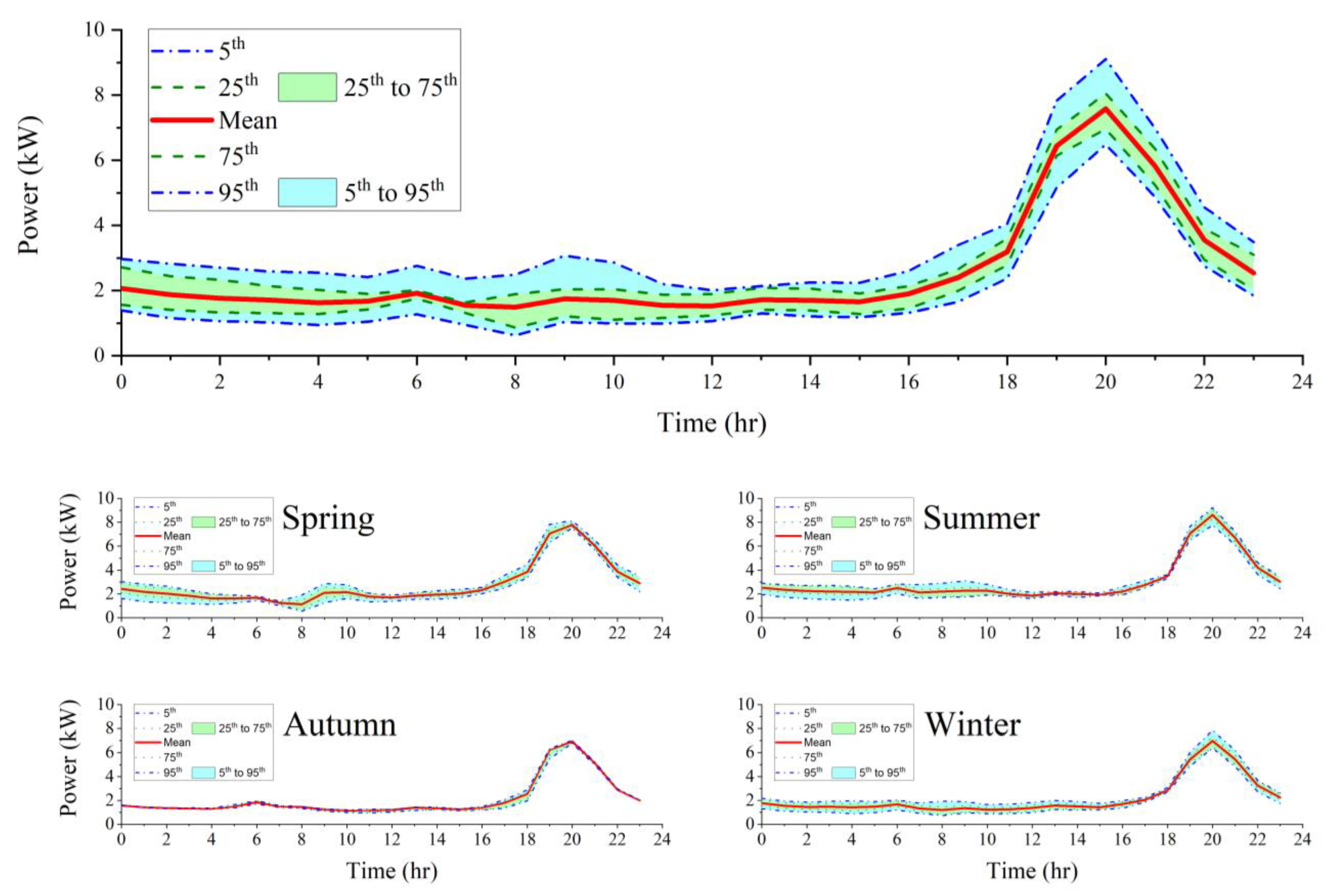
4.1. Demand of Residential Customers

Based on the hourly electricity metering data, available for a period of around two years, the demands of the 374 single-phase connected households were aggregated into a lumped residential load and modelled as a balanced three-phase voltage-independent “constant PQ power” load type, represented by the corresponding average annual and seasonal daily demand load profiles, together with the corresponding 5th, 25th, 75th, and 95th percentiles.

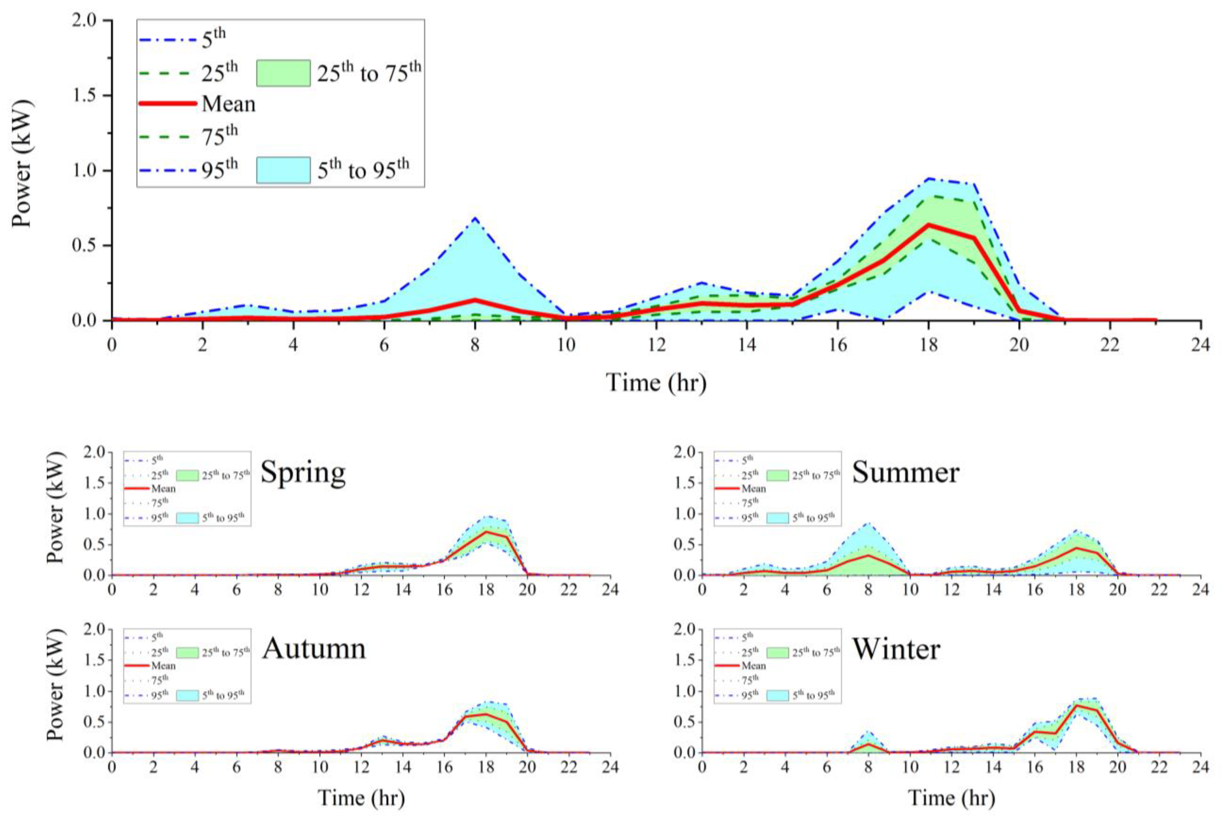
4.2. Demand of PUEs Customers

Similarly, using the available hourly electricity metering data for the PUE loads, the average annual and seasonal daily load profiles (with 5th, 25th, 75th, and 95th percentiles), for three types of PUEs (i.e., chicken brooders, EV charging stations, and posho mills) were identified and used for modelling as three-phase balanced “constant PQ power” loads.

4.3. Total Mini-Grid Demand

Utilizing mini-grid hourly readings of all residential and PUE customers for one year, their average daily and peak demands, together with 5th, 25th, 75th, and 95th percentiles, are calculated. Figure 16 and Figure 17 show average annual and seasonal total mini-grid demands and residential load demands (with percentile ranges), respectively. Similarly, the average annual and seasonal daily demands, as well as their percentile ranges, for EV charging stations are shown in Figure 18, while Figure 19 and Figure 20 show these values for the posho mills and chicken brooders PUE loads, respectively.

Electricity demand for lighting and home appliances (e.g., cooking, TVs, refrigerators, etc.) accounts for the majority of mini-grid households’ energy use. The peak demand of the total mini-grid load happens in the evening, as Figure 16 illustrates. This is due to the peak and bulk of residential demand, Figure 17, occurring in the evening, when solar energy is not available, leading to a heavy reliance on the mini-grid battery storage. By exploiting the flexibility of the residential demand, non-critical or flexible loads can be moved to off-peak times, thus maximizing the use of available solar PV generation and improving the overall mini-grid load factor (e.g., through promoting the use of electric cookers). The same concept of load shifting may be applied to different types of PUEs, such as posho mills and chicken brooders, where peak evening demand appears to coincide with the residential load, as shown in Figure 19 and Figure 20, respectively.

The demand for EV charging stations, however, is primarily present during the day, suggesting that controlled daily-charging of EV batteries (the EVs are operated on a battery-swapping regime) helps to make up for the off-peak demand of residential and other PUE customers and to maximize the use of available solar energy. However, there is a sizeable EV demand in the evening in Figure 18, when mini-grid battery storage is used, which is possibly due to the need to charge all available batteries (including those returned in the evening after the use on the current day) for planned activities on the next day.

Figure 19 shows that, for the majority of the year, posho mills demand peaks in the evening, coinciding with the demand for residential load. Additionally, Figure 20 shows that the demand of the chicken brooders mostly occurs during the night-hours, when PV generation is not available (the brooders were field-trialled within the community for a limited period of time, and this demand was absent in autumn when the brooders were not active in the provided dataset). Such a load profile competes with household energy demand during the night and requires additional storage capacity if the number of brooders is to be increased in the future.

5. Modelling of Renewable Energy Resources

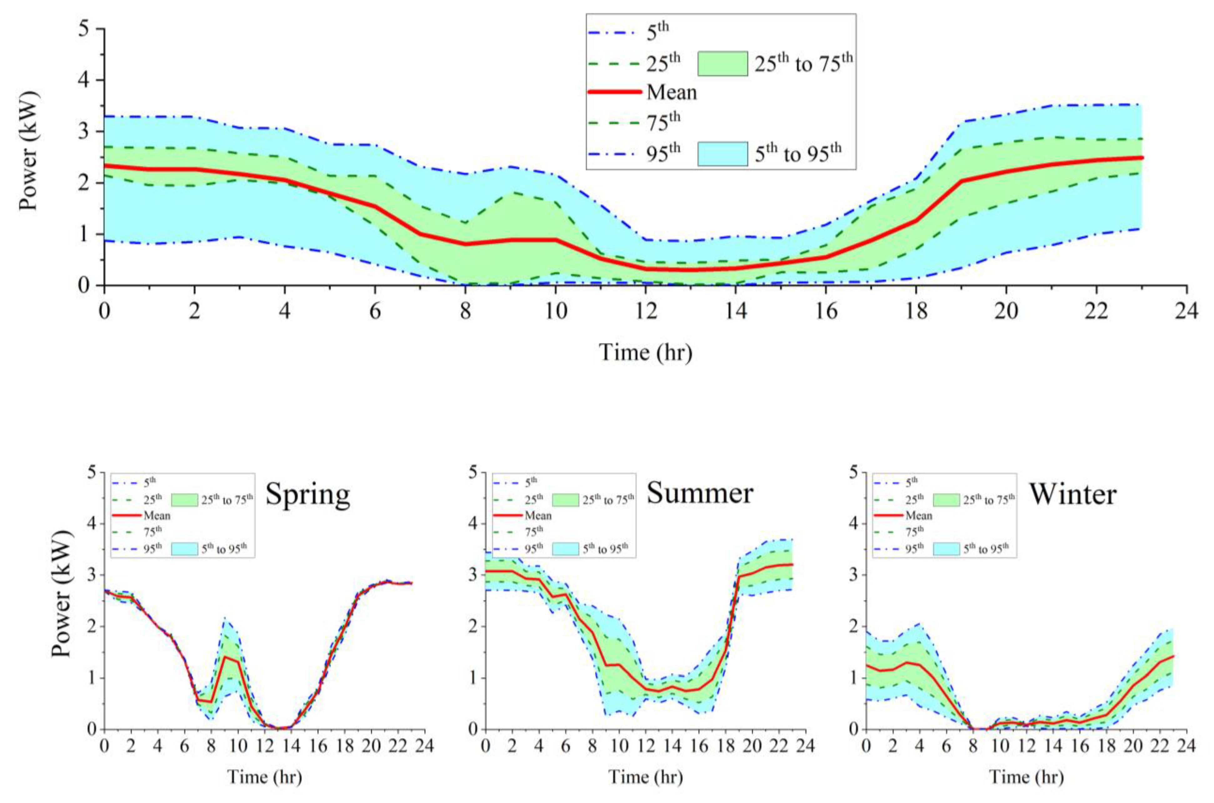
5.1. Solar Irradiance

Daily and seasonal variations of solar energy resources, i.e., solar irradiance, generally follow predictable patterns, but they are typically strongly impacted by the local weather conditions, e.g., cloud coverage, precipitation, temperature variations, etc., which then introduce uncertainties in the power outputs of PV generation systems. This highlights the importance of assessing related weather conditions for the correct evaluation of the variations and uncertainties in the PV system output powers, which can be done either by using local measurements of weather data or by extracting these data from some of the available solar irradiance calculators/databases, e.g., from [23].

As no weather data, including solar irradiance, were available at the location of the modelled mini-grid, the solar irradiance data from [23] are used for the analysis, where global horizontal irradiance (GHI) data, at a 15 min resolution, are upscaled to 1 h average values, imported into the model, and used to run mini-grid simulations.

5.2. Ambient Temperature and Other Meteorological Parameters

The same weather database [23] was used to retrieve other meteorological data, including ambient temperature and cloud opacity, with an overview of average monthly values for 2021 given in

Table 6. Monthly average values of GHI, ambient temperature, and cloud opacity, as well as sunrise and sunset times at the beginning of the month, for the modelled Gionseri B mini-grid site.

Year 2021	Air Temperature (°C)	GHI (W/m2)	Cloud Opacity (%)	Sunrise Time	Sunset Time
January	18.4	221.1	45.8	06:46	18:53
February	19.1	235.1	45.9	06:51	18:57
March	19.6	260.2	42.5	06:46	18:51
April	17.6	230.7	54.9	06:38	18:42
May	17.0	217.6	41.7	06:35	18:38
June	16.9	226.1	31.3	06:39	18:42
July	16.9	207.1	37.9	06:44	18:47
August	17.9	224.6	36.4	06:42	18:46
September	17.8	218.2	46.2	06:33	18:37
October	18.7	236.9	43.0	06:23	18:29
November	18.7	232.6	44.0	06:22	18:29
December	18.1	207.2	46.9	06:32	18:40

(the main rain season is in the April–May period).

6. Results and Validation

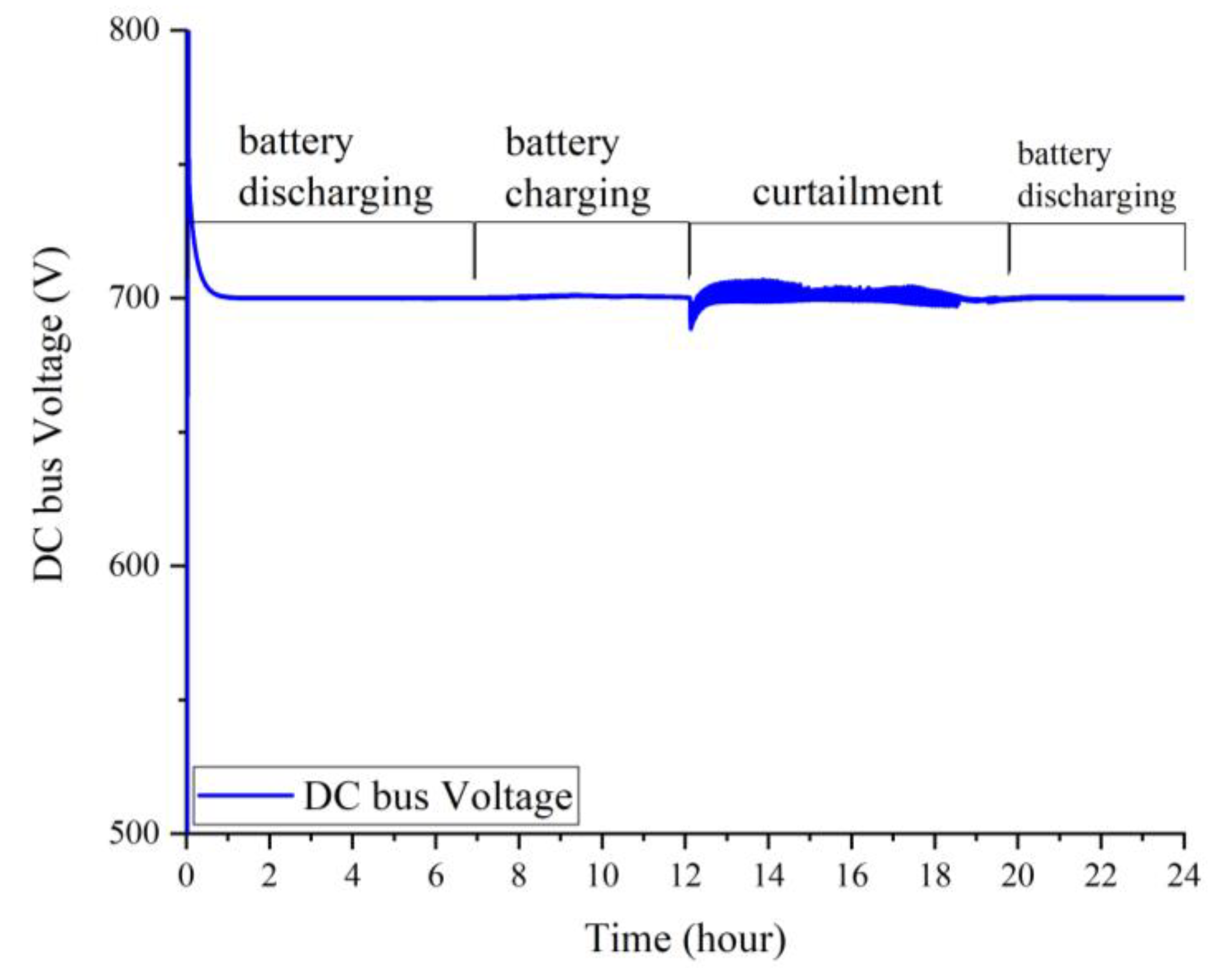
6.1. Validation of Mini-Grid Inverter Model

Figure 21 and Figure 22 show, respectively, the simulation results for the mini-grid inverter/filter operation (voltage and current waveforms before and after the filter) and for the controlled DC bus voltage. As can be seen in Figure 21, the operation of the implemented dq-frame control of the three-phase off-grid inverter is as expected, while the results for the voltage/current output of the LCL-type filter (i.e., transformer output) demonstrates that it meets the necessary power quality requirements for supplying loads connected to the mini-grid. Figure 22 shows that the DC bus voltage remains stable throughout the 24 h simulation period and for the different mini-grid operation modes, such as battery charging/discharging and PV curtailment.

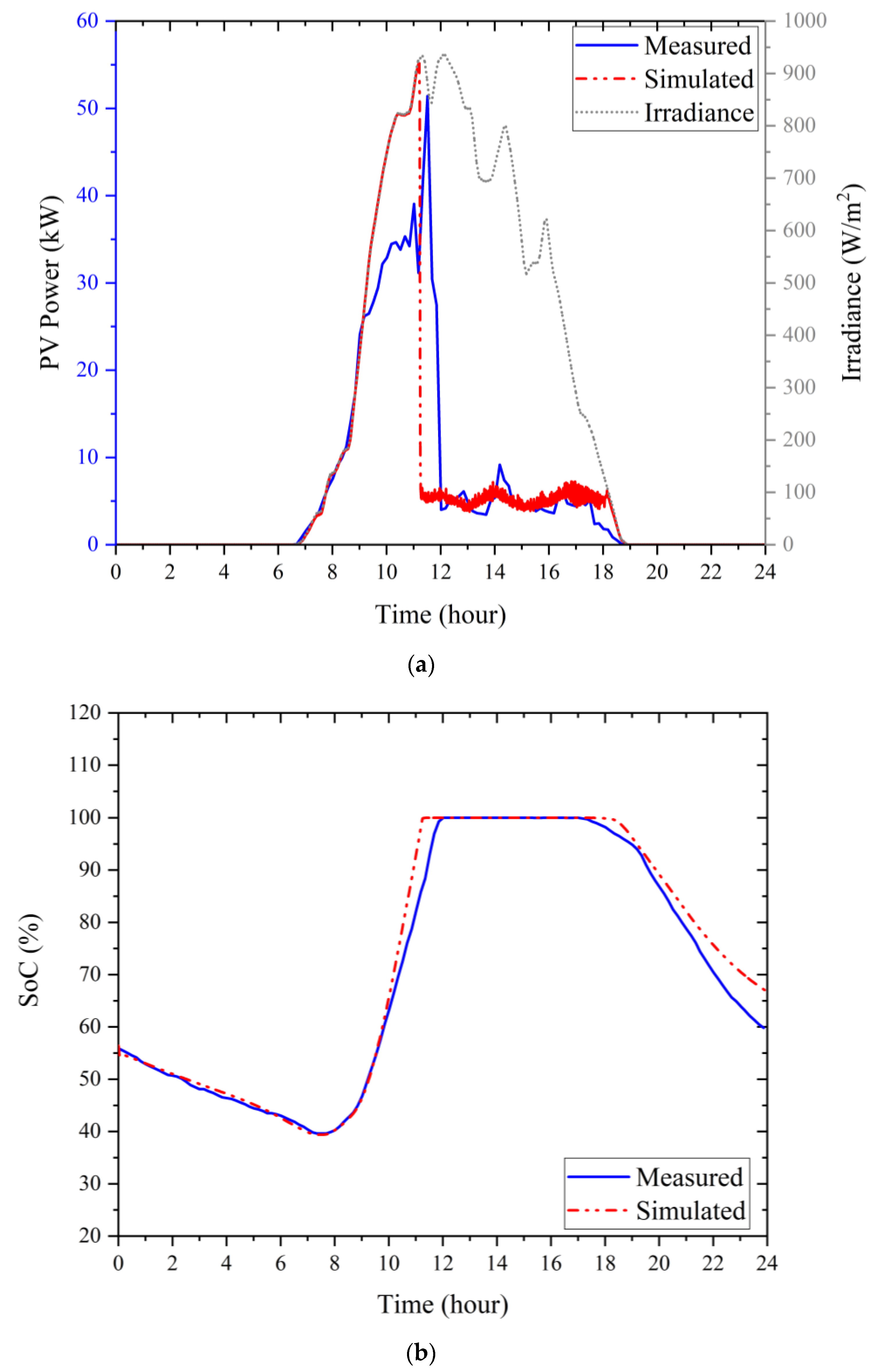
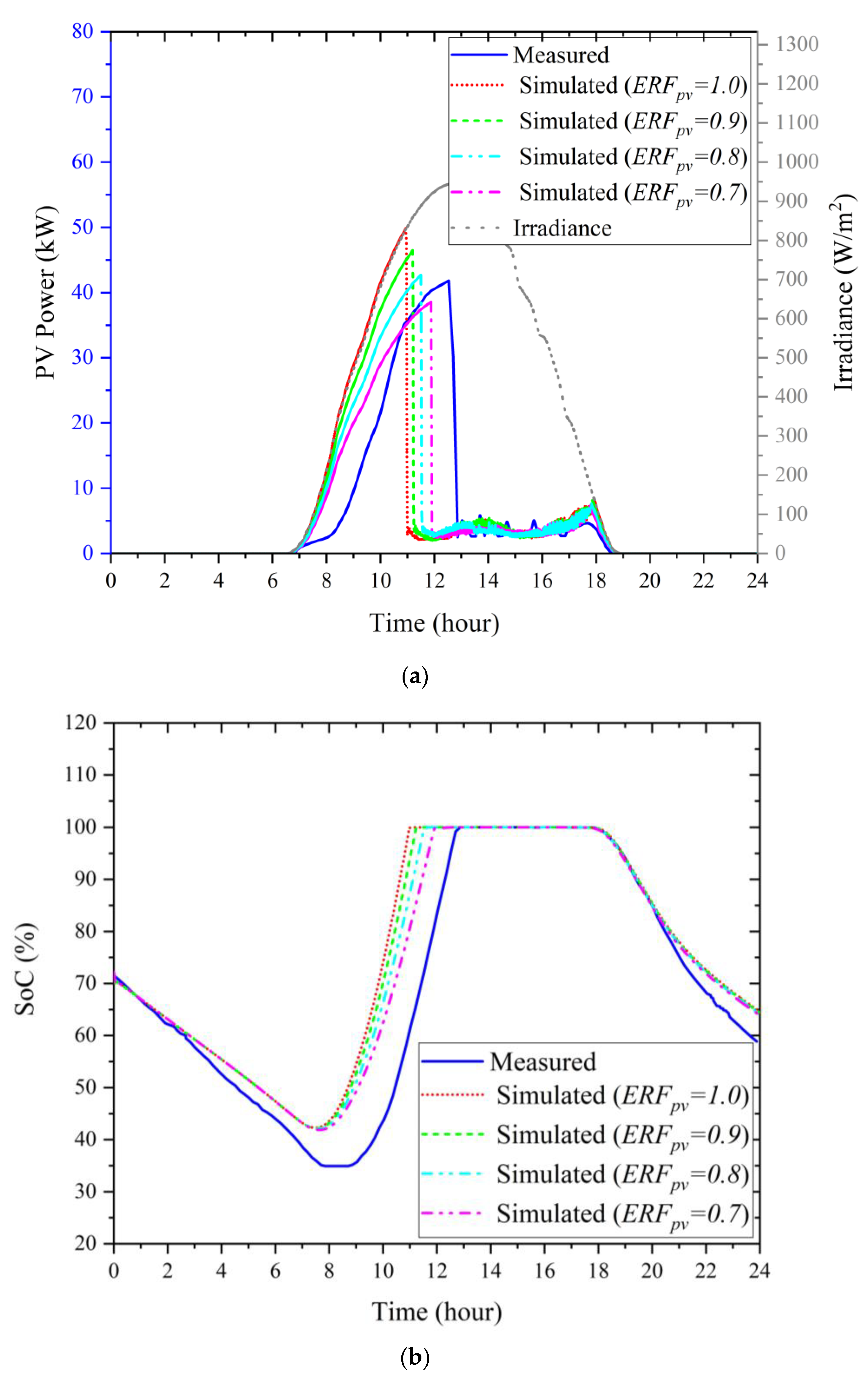
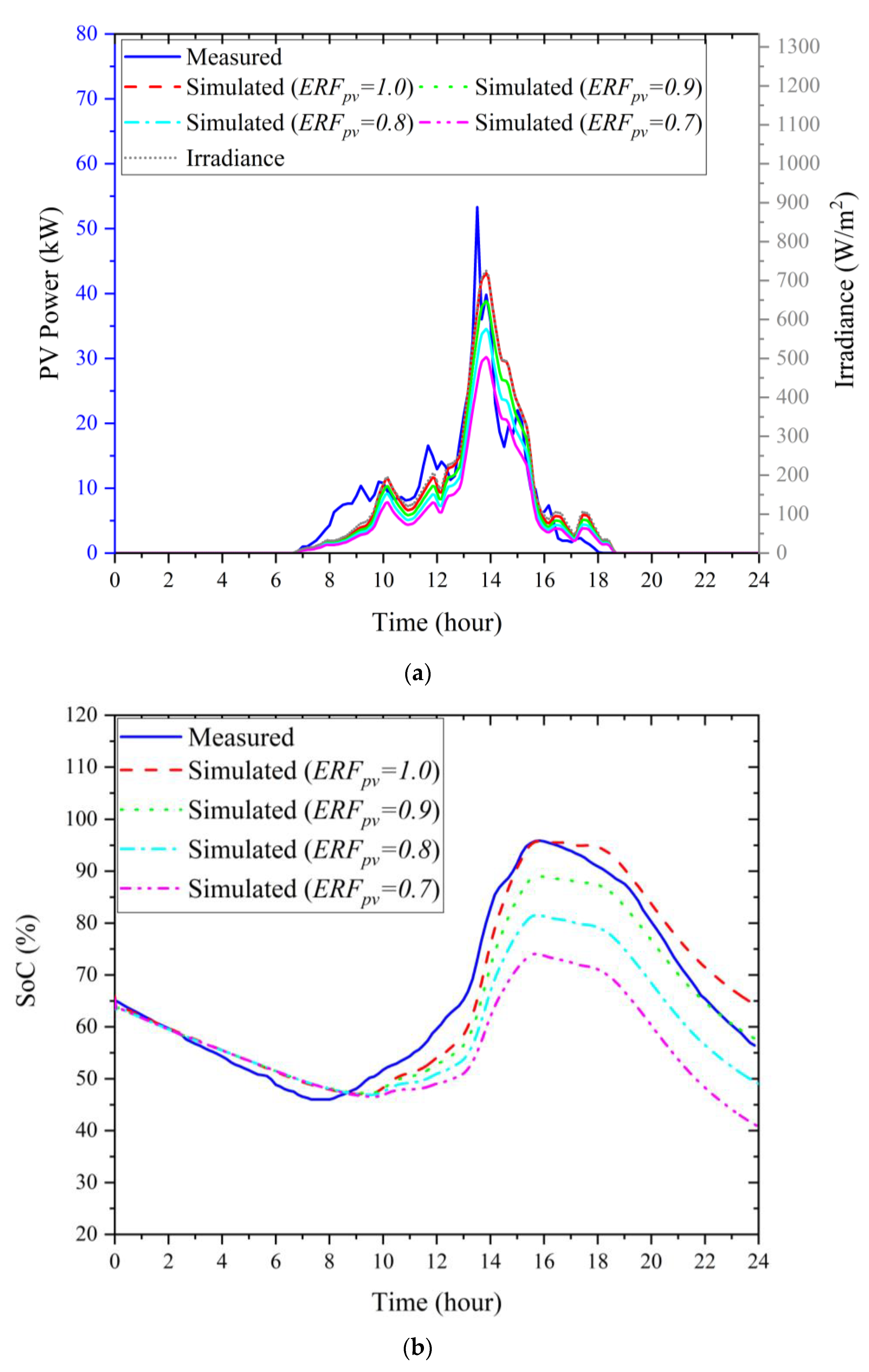
6.2. Validation of Mini-Grid PV System and Battery Storage Models

In order to validate the developed mini-grid model, this section compares the results of simulations with the actual mini-grid measurements. The first set of results is related to a day with a combination of clear sky and cloudy sky conditions. As seen in Figure 23-a, the simulation results closely align with recorded data until around 09:30 h, when the energy management system (EMS) starts to limit some of the available PV power before the battery reaches 100% SoC. As the full information on the EMS control settings that impact this PV curtailment was not available, it was not possible to include related controls in the developed mini-grid model. However, outside of the partial PV curtailment period in Figure 23-a (09:30–12:00 h), the mini-grid model simulation results closely match the logged EMS measurements in terms of PV generation and battery voltage, as well as current and SoC. It is worth noting that, as Figure 23 shows, significant curtailment of available PV generation is initiated when battery SoC reaches 100%, which is confirmed by both the simulation results and the actual measurements.

Figure 24 presents another comparison of simulation results with actual EMS measurements for a clear sunny day. As Figure 24-a illustrates, even though the weather conditions are clear sky on a sunny day (solar irradiance is plotted by a black dotted line), the actual PV production (blue solid line) is lower than the simulated PV production (red dotted line). Due to the absence of on-site measurements of solar irradiance, PV panel temperature, battery temperature, etc., which might have caused a decrease in the measured PV outputs, the actual reasons for the reduced PV power output could not be confirmed. Furthermore, internal control settings of the EMS are also unknown and, therefore, not modelled, although they could be based on some parameters (e.g., multi-stage charging of the battery, battery temperature, etc.) that may limit/curtail the available PV power before the battery reaches full capacity (e.g., to prevent overcharging of the battery, to extend the lifetime of the battery, or to avoid safety issues related to the increase in battery temperature).

In the absence of on-site measurements of weather data and full information on the settings of the EMS controls, the variations and uncertainties in the PV output power are modelled by introducing “empirical reduction factor” (ERF_pv), which is, in Figure 24, compared for the base case (“ERF_pv = 1.0”, red line) and for three cases with reduced PV power outputs (“ERF_pv = 0.9”, green dashed line, “ERF_pv = 0.8”, light-blue dash-dotted line, and “ERF_pv = 0.7”, maroon dash-dotted line).

A further discrepancy can be seen at the start of the day in Figure 24b, when solar irradiance taken from [23] and shown in Figure 24a with a dotted black line starts to raise, but the measured PV output power (solid blue line) does not increase proportionally with it. Instead, the gradient of the increase in the measured PV power output is lower at the start of the day, which also coincides with the change of battery operating mode from discharging to charging: the start of the battery charging in the simulation is around one hour before it is indicated by the actual measurements (which also show a period when the battery is “idling”, i.e., neither charging nor discharging). This “delay” of the measured SoC data with respect to the simulated SoC values, which is due to a lower generated PV power than what it should be based on the available solar irradiance, will result in the battery reaching 100% SoC later in the day, as compared to the simulation results in Figure 24b. A possible reason for the measured PV output power curve having a different gradient at the start of day could be that the MPPT is activated some time afterwards. Although the available EMS data are not sufficient to confirm this possible cause (no measured solar irradiance and no continuous DC voltage measurements were available), it was found, by visiting the mini-grid site, that the DC voltage level adjusted by the EMS at the start of the day is lower (around 530 V) than the expected MPP voltage (around 660 V), i.e., the PV panels are operated in the constant current region of their I–V curves, thereby producing lower power output than the one corresponding to the estimated input solar irradiance.

Figure 25 further compares results for a combined clear sky and cloudy sky day from Figure 23 with two ERF_pv values of 1.0 and 0.8. The simulation results in Figure 25a with ERF_pv = 1.0 are a better match to the measured PV output power for the period from the start of the charging cycle until the SoC of the battery (Figure 25b) is around 50%, as compared to the simulations with ERF_pv = 0.8. Afterwards, however, the simulation results with ERF_pv = 0.8 show better matching, and they correctly indicate when battery charging stops (i.e., when battery SoC is 100%). This suggests that a suitable ERF_pv should be implemented only after the battery reaches a threshold SoC.

As mentioned, the data on actual solar irradiance and set points of the EMS controls are not available, and the most likely reason for a partial curtailment of the PV power output, in this case, is thought to be the adjustment of the lower battery charging current/power in order to limit the increase in battery temperature. In other words, on a clear day (not on a cloudy day), the battery temperature will increase much faster when the sky is clear, and maximum solar irradiance results in maximum charging current, which should be reduced to prevent an excessive increase in battery temperature. In order to check that assumption, the next considered example is a full cloudy day in Figure 26.

For a whole day with cloudy sky in Figure 26, the battery SoC did not reach 100% during the day due to the lower solar irradiance levels on the PV panels caused by cloud coverage. This is, mostly, correctly indicated by the weather database results for solar irradiance from [23] (black dotted line). Importantly, there is no need to apply ERF_pv values lower than unity on this day, as for most of the day, charging currents are low and, therefore, not expected to result in excessive increase of battery temperature. It should be noted again, however, that the presented simulation results may not fully reflect the real conditions at the mini-grid site, as they are based on inputs from a satellite-based weather database in [23], which may not correctly account for location-specific factors, such as cloud coverage, presence of obstructions casting shadows on the PV panels, albedo effect, and scattered light at the actual mini-grid site. Nevertheless, the presented results clearly indicate the importance of including temperature dependency and other relevant thermal aspects in both the PV system model and battery energy storage model, either directly—when related measurement data are available,—or indirectly—when empirical-based or otherwise identified adjustment factors are used—as presented in this paper.

To illustrate the benefits of using appropriate empirical adjustment factors such as ERF_pv in this paper,

Table 7. The RMS and MAPE indices for simulation models with different ERF_pv values on the considered days.

Case	ERFpv	PV Power			Battery SoC
		RMSE	MAPE (%)	ΔEn * (kWh)	RMSE	MAPE (%)
Combined Clear/Cloudy Day	1.0	6.72	12.15	7.35	3.33	2.60
	0.9	5.59	10.70	6.55	2.52	2.09
	0.8	2.73	9.72	5.50	2.03	1.92
	0.7	3.72	10.31	4.01	2.67	2.55
Clear Day	1.0	11.98	17.27	−4.52	11.77	12.17
	0.9	10.74	16.82	−4.33	10.71	11.24
	0.8	9.38	15.13	−5.79	9.43	10.17
	0.7	7.74	12.76	−7.52	7.85	8.94
Cloudy Day	1.0	2.87	13.17	1.61	3.88	4.78
	0.9	2.76	14.07	−12.11	4.30	4.83
	0.8	3.09	16.61	−25.718	8.69	9.49
	0.7	3.74	18.36	−39.17	13.62	14.21

* ΔEn = Simulated PV energy production—Measured PV energy production.

compares different error metrics, root mean square error (RMSE), mean average percentage error (MAPE), and the difference between simulated and metered energy production (ΔEn) for the three considered days with different weather conditions. The lower values of all error indices represent better matching of simulation results with specific ERF_pv values and measured values, but they are not conclusive indicators of a better model.

Based on the values in Table 7, particularly regarding energy production results, the best match of simulation results with the measurements is obtained for ERF_pv = 0.8 on clear and combined clear–cloudy days, as well as for ERF_pv = 1 on cloudy days.

7. Evaluating Options for Mini-Grid Extension and Connection of New Customers

Figure 27a shows that, primarily due to a low total mini-grid demand, available PV power output is regularly curtailed (“wasted”) after the battery is fully charged, which typically happens around noon (12:00 h). This means that there is significant spare capacity in the existing mini-grid system to connect new loads (e.g., residential or PEU customers), which is analysed in this section. The original oversizing of a mini-grid can often be explained by overreliance on energy use surveys, which tend to substantially exaggerate actual consumption of electricity [15], or simply by more favourable financing and procurement terms, from the point of view of the installer, based on scale and on projected expansion of customer base [24].

In the further text, the potential of the Gionseri B mini-grid for connecting additional load (residential or PUE customers) is evaluated using daily load profiles from Section 4 for two cases: (a) based on the calculated annual average daily demand and (b) based on the specific day of the peak demand.

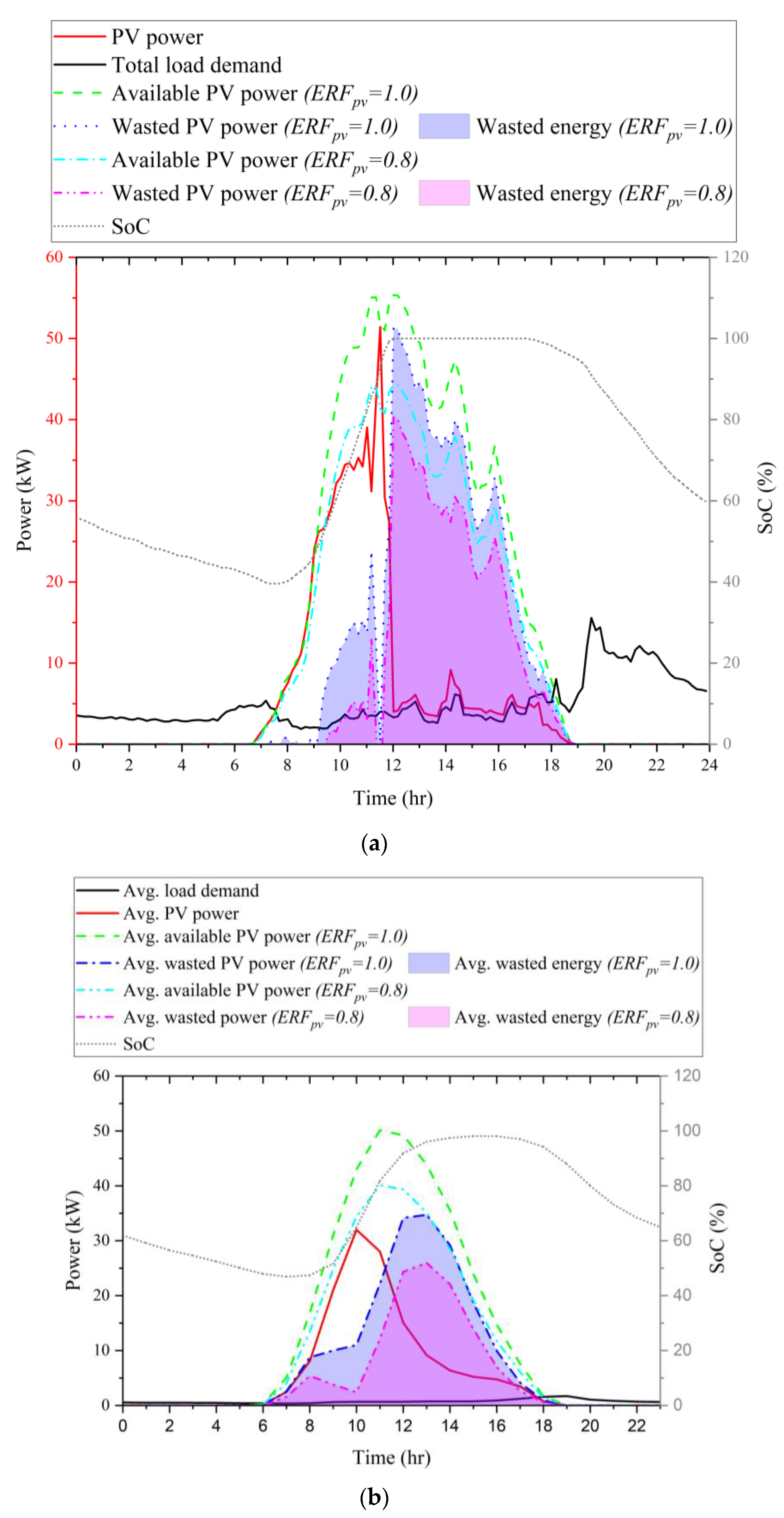
7.1. Mini-Grid Potential for Connecting New Customers Based on Annual Average Daily Profiles

Using solar irradiance data from [23] and models developed in the previous sections, the expected annual average daily energy production for the Gionseri B mini-grid site is 323 kWh for ERF_pv = 1 and 258 kWh for ERF_pv = 0.8, while the actual annual average daily energy production is 125 kWh. Accordingly, around 198 kWh (for ERF_pv = 1) and around 133 kWh (for ERF_pv = 0.8) are not used due to a low demand, resulting in significant daily PV generation curtailment after the battery storage reaches 100% SoC. This is illustrated in Figure 27a using recorded data for the same day as in Figure 23, as well as in Figure 27b using annual average daily profiles. In both cases, due to a relatively low total mini-grid demand (red line), the battery reaches 100% SoC at around noon (green line), and it stays there until late afternoon/early evening hours (until PV output reduces due to low solar irradiance), allowing for the evaluation of “curtailed power” (maroon line) and “curtailed energy” (light-blue shaded area), which is evident from a comparison of “available PV power” (blue line) and “actual PV power” (black line).

Equation (18) is used to estimate the maximum number of additional residential or PUE customers that can be connected to the existing mini-grid based on the annual average daily energy use, as shown in

Table 8. Maximum number of new residential and PUE customers using annual average daily demand (the first value in the last column is for ERF_pv = 1, while the second value is for ERF_pv = 0.8).

Customer Type	No. of Existing Customers	Average Daily Energy Used by One Customer	No. of New Customers that Could Be Connected (Each Type Excluding the Others)
Residential	374 houses	0.114 kWh	1730/1166 houses
EV Charging	1	6.936 kWh	28/19
Posho Mills	2	1.512 kWh	130/88
Chicken Brooders	3	3.152 kWh	62/42

.

$$N_{ce}=\frac{E_{dc}}{E_{dd}}$$

(18)

where $N_{ce}$ is the maximum number of new customers that can be connected using average daily demand, $E_{dc}$ is the average daily curtailed (or “wasted”) energy, and $E_{dd}$ is the average daily energy demand by load type.

7.2. Mini-Grid Potential for Connecting New Customers Based on Rated System Power and Peak Demand

Based on the PV mini-grid maximum/rated power capacity and peak demand of specific types of customers, Equation (19) can be used to estimate the maximum number of residential and PUE customers that can be connected to the existing mini-grid, as shown in

Table 9. Maximum number of new customers using peak power demand values.

Customer Type	Maximum Power Demand by a Single Customer	No. of New Customer that Could Be Connected (Each Type Excluding the Others)
Residential	Shared Peak: 12 kW/374	987 houses
	Single Peak: 1738 W	16
EV Charging	4032 W	7
Posho Mills	2120.5 W	14
Chicken Brooders	4247 W	7

.

$$N_{pe}=\frac{P_{rated}-P_{pload}}{P_{pd}}$$

(19)

where $N_{pe}$ is the maximum number of new customers operating at their peak demand; $P_{rated}$ is the rated power of the inverter (i.e., 50 kW); $P_{pload}$ is the peak demand of the total load; $P_{pd}$ is the power demand of the considered load type.

7.3. Discussion of Socio-Behavioural Aspects Influencing Design and Operation of Mini-Grids

Beyond the technical analysis provided in this paper, social aspects loom large in the data and in the recommendations that could be made. As an example, the daily demand profiles of posho mills identified in Figure 19 suggest a pattern of operation that is poorly matched with available daily solar irradiance resource. The possible reasons might be that posho mills are used for the processing of the harvest gathered or bought during the day and then brought for milling in the evening, or it may be that the mill operators have other duties during the day and are only available in the evening. This suggests that suitable changes in electricity demands, e.g., to follow more closely to available solar energy resources, might first require socio-behavioural changes related to the activities performed by the involved community members. These and other related aspects will be analysed in a follow-up paper, which will explore socio-behavioural context of energy use in Kenyan mini-grids, including their analysis through the lens of Gender Equality and Social Inclusion.

8. Discussion and Conclusions

8.1. Discussion of the Presented Analysis and Results

After presenting an overview of typical Kenyan PV mini-grid applications and average daily load profiles of the residential and PUE customers that are identified from the measured demands, the paper introduces the main mini-grid components and their models, including a simple, yet reasonably accurate, model of a mini-grid battery storage system based on the manufacturer’s battery charge–discharge curves. All mini-grid components are then assembled in a scalable and easily reconfigurable simulation model of an actual Kenyan PV mini-grid. Afterwards, the developed simulation model is validated using available measurement data and implemented for the evaluation of PV mini-grid performance, potential for expansion, and connection of additional residential and PUE customers. The presented PV mini-grid model can be used for further analysis, such as to study techno-economic performance of different mini-grid configurations, to identify optimal sizing of mini-grid components, and to specify efficient control and operation schemes based on the locally available resources.

The initial comparison of the results of PV mini-grid simulations with available measurements confirmed that the simulations follow the overall patterns of the recorded mini-grid data. However, due to the unavailability of information on the actual control algorithms and control settings of the mini-grid energy management systems, as well as the absence of on-site weather data (most importantly, measurements of input solar irradiance), the initial simulation results obtained using a satellite imagery weather database did not fully match the recorded data. Therefore, a suitable empirical approach for adjusting the PV system output power (on clear days but not on cloudy days) is presented and discussed in terms of the improved model accuracy.

The presented results also indicate the importance of the correct modelling of thermal dependencies and characteristics of both PV generation systems and battery storage systems. Although the thermal models of the PV generation and battery systems are not considered in the presented analysis, with the main reason, again, being that the information about the relevant thermal parameters was not available, this is a subject of the further work by the authors in the RESILIENT project.

8.2. Main Conclusions

In Kenya, PV mini grids are recognized as a feasible and, often, only practical solution for meeting the government’s long-term development plan for increased electricity access in remote and scattered rural areas. Low electricity demands, however, pose a major barrier to the financial viability of mini-grids, ultimately limiting their potential for the provision of a sustainable, reliable, and affordable energy supply.

Low electricity demand in rural mini-grids can be attributed to several factors. One of the main reasons is the low income of the households, i.e., their inability to afford the costs associated with using electricity from the mini-grids. Another reason is that many households in rural areas still rely on the use of traditional energy sources, such as firewood for cooking and kerosene for lighting, which, in practice, reduce electricity demands in mini-grids. Low mini-grid demands highlight the importance of a careful evaluation of the energy needs of residential and small commercial customers during the mini-grid planning and design stages, as well as even more careful evaluation of the options for increasing the demands from existing customers, for assessing the potential for connecting new customers, and for extension into a multi-vector energy supply during the mini-grid operational stage. This paper considered these aspects of the analysis of mini-grids and presented the details of the development of a versatile simulation model of an actual mini-grid in Kenya, which was also validated using the measurement data available from RESILIENT project.

It should be noted that RESILIENT project considers deployment of multi-vector mini-grids, integrating electrical, thermal, transport, and other energy vectors into typical PV mini-grid systems. This approach can stimulate new demand for electricity, as it enables the provision of a wider range of essential services, such as those for water purification, heating, cooling, and transportation, and it allows for local development through the PUE activities. Additionally, the integration of renewable-based energy vectors can allow for a significant decarbonisation through a much higher utilisation of locally available energy resources, which will then help to reduce the costs associated with mini-grid electricity generation and distribution. This, in turn, will help to address poverty in rural communities by lowering electricity tariffs through the increased mini-grid revenues, making electricity supply in mini-grids more affordable. Finally, socio-economic aspects, in the context of the specific community where the mini-grid is installed, must be carefully considered, both regarding the interpretation of the data and in terms of the designs of mini-grids that will maximise utilization of the resources by combining different energy vectors in target generation and the storage system, by integrating suitable PUE activities, and by offering incentives to customers for adopting different patterns of energy use.

At the time of writing this paper, field trials in selected pilot mini-grid communities in RESILIENT project are ongoing. After the three selected trials end and after the collected information and measurement data are processed (the three trials are, respectively, related to: using electric vehicles/bikes for transporting goods and people; combining electrical and thermal energy generation and storage; adding a water purification plant to an existing PV mini-grid), benefits of deploying multi-vector energy systems will be evaluated in more detail and reported in a separate paper.

References

1. Kenya Vision 2030 Flagship Programmes and Projects Progress Report (FY 2020/2021). Kenya Vision 2030. Aug. 2022. Available online: https://vision2030.go.ke/publication/kenya-vision-2030-flagship-programmes-and-projects-progress-report-fy-2020-2021/ (accessed on 15 December 2022).
2. Kenya National Electrification Strategy: Key Highlights 2018. Available online: https://pubdocs.worldbank.org/en/413001554284496731/Kenya-National-Electrification-Strategy-KNES-Key-Highlights-2018.pdf (accessed on 15 December 2022).
3. African Energy Outlook 2022. Development Policy and Performance Portal. Available online: https://development.finance.go.ug/knowledge-centre-reports/african-energy-outlook-2022 (accessed on 5 December 2022).
4. Antonanzas-Torres, F.; Antonanzas, J.; Blanco-Fernandez, J. State-of-the-Art of Mini Grids for Rural Electrification in West Africa. Energies 2021, 14, 990. [Google Scholar] [CrossRef]
5. van Hove, E.; Johnson, N.; Blechinger, P. Evaluating the impact of productive uses of electricity on mini-grid bankability. Energy Sustain. Dev. 2022, 71, 238–250. [Google Scholar] [CrossRef]
6. Liu, Y.; Bah, Z. Enabling development impact of solar mini-grids through the community engagement: Evidence from rural Sierra Leone. Energy Policy 2021, 154, 112294. [Google Scholar] [CrossRef]
7. ESMAP. Mini Grids for Half a Billion People: Market Outlook and Handbook for Decision Makers; Executive Summary; Energy Sector Management Assistance Program (ESMAP) Technical Report 014/19; World Bank: Washington, DC, USA, 2019. [Google Scholar]
8. Contejean, A.; Verin, L. Making Mini-Grids Work: Productive Uses of Electricity in Tanzania. International Institute for Environment and Development, 2017. Available online: https://www.iied.org/16632iied (accessed on 5 January 2023).
9. Kirubi, C.; Jacobson, A.; Kammen, D.; Mills, A. Community-Based Electric Micro-Grids Can Contribute to Rural Development: Evidence from Kenya. World Dev. 2009, 37, 1208–1221. [Google Scholar] [CrossRef]
10. Zebra, E.I.C.; van der Windt, H.; Nhumaio, G.; Faaij, A.P.C. A review of hybrid renewable energy systems in mini-grids for off-grid electrification in developing countries. Renew. Sust. Energ. Rev. 2021, 144, 111036. [Google Scholar] [CrossRef]
11. Emad, D.; El-Hameed, M.; El-Fergany, A. Optimal techno-economic design of hybrid PV/wind system comprising battery energy storage: Case study for a remote area. Energy Convers. Manag. 2021, 249, 114847. [Google Scholar] [CrossRef]
12. Mokhtara, C.; Negrou, B.; Bouferrouk, A.; Yao, Y.; Settou, N.; Ramadan, M. Integrated supply-demand energy management for optimal design of off-grid hybrid renewable energy systems for residential electrification in arid climates’. Energy Convers. Manag. 2020, 221, 113192. [Google Scholar] [CrossRef]
13. Hartvigsson, E.; Ehnberg, J.; Ahlgren, E.; Molander, S. Linking household and productive use of electricity with mini-grid dimensioning and operation. Energy Sustain. Dev. 2021, 60, 82–89. [Google Scholar] [CrossRef]
14. Bhattacharyya, S. Mini-grid based electrification in Bangladesh: Technical configuration and business analysis. Renew. Energy 2015, 75, 745–761. [Google Scholar] [CrossRef] [Green Version]
15. Blodgett, C.; Dauenhauer, P.; Louie, H.; Kickham, L. Accuracy of energy-use surveys in predicting rural mini-grid user consumption. Energy Sustain. Dev. 2017, 41, 88–105. [Google Scholar] [CrossRef] [Green Version]
16. The MathWorks, I. Simulink, Natick, Massachusetts, United State. 2022. Available online: https://uk.mathworks.com/help/simulink/ (accessed on 15 October 2022).
17. Canadian Solar MaxPower CS6U-330P. Available online: https://ourolux.com.br/media/sparsh/product_attachment/Datasheet_M_dulo_330W_-_Canadian_-_CS6U330P.pdf (accessed on 1 October 2022).
18. PV Array. Implement PV Array Modules—Simulink. Available online: https://uk.mathworks.com/help/sps/powersys/ref/pvarray.html;jsessionid=1af41c5c3fe0b10a1fe9cba7a774 (accessed on 1 November 2022).
19. BATTERY M38210-S Model. Available online: https://www.alphaess.com/Public/Uploads/uploadfile/files/20220620/Datasheet_EN_M38210-S_V06.07092021.pdf (accessed on 1 October 2022).
20. Simulink Generic Battery Model. Available online: https://uk.mathworks.com/help/sps/powersys/ref/battery.html (accessed on 1 November 2022).
21. Timlee, Eve LF105 3.2V 105ah Lifepo4 Battery Cell Specification (Datasheet). Energie Panda, 12 January 2022. Available online: http://www.dcmax.com.tw/LF105%283.2V105Ah%29.pdf (accessed on 15 November 2022).
22. East African Cables, Table39 100.0sq XLPE-AAC. Available online: https://www.eacables.com/images/eac_technical_brochure_new.pdf (accessed on 20 November 2022).
23. SolCast, Solar Forecasting and Modelling Based on Weather Satellite Imagery. Available online: https://solcast.com/ (accessed on 12 September 2022).
24. Agenbroad, J.; Kelly, C.; Kendall, E.; Stephen, D. Minigrids in the Money: Six Ways to Reduce Minigrid Costs by 60% for Rural Electrification. Rocky Mountain Institute. 2018. Available online: www.rmi.org/insight/minigrids2018 (accessed on 15 February 2023).
Figure 1. Mini-grid (a) layout; (b) single-line diagram (Gionseri B site in Kenya).
Energies 16 03203 g001
Figure 2. Comparison of PV panel characteristics from manufacturer data in [17] (solid lines) and the simulation model (dash-dot lines), for I–V characteristics, at (a) different solar irradiance levels; (b) different ambient temperatures.
Energies 16 03203 g002
Figure 3. Thévenin equivalent circuit of the battery model.
Energies 16 03203 g003
Figure 4. Variations in battery terminal voltage for different charge–discharge currents: (a) manufacturer data [12]; (b) simulation results.
Energies 16 03203 g004
Figure 5. Polynomial curve fittings: (a) internal series resistance; (b) open-circuit voltage.
Energies 16 03203 g005
Figure 6. Implemented model of the battery pack.
Energies 16 03203 g006
Figure 7. Model of the PV-side DC–DC boost converter.
Energies 16 03203 g007
Figure 8. Block diagram of the control system for boost converter interfacing PV system and DC bus.
Energies 16 03203 g008
Figure 9. The P&O MPPT algorithm.
Energies 16 03203 g009
Figure 10. Model of the battery bi-directional boost converter.
Energies 16 03203 g010
Figure 11. Block diagram of battery controller.
Energies 16 03203 g011
Figure 12. Model of the split DC link three-phase, four-wire inverter topology.
Energies 16 03203 g012
Figure 13. Block diagram of inverter controller.
Energies 16 03203 g013
Figure 14. The LC low-pass filter schematics: (a) without transformer; (b) with transformer acting as the load-side inductor and forming the resulting LCL-type filter.
Energies 16 03203 g014
Figure 15. A map representation of the distribution network of the modelled mini-grid.
Energies 16 03203 g015
Figure 16. Average annual and seasonal whole mini-grid (total) daily demand load profiles (with percentile ranges).
Energies 16 03203 g016
Figure 17. Average annual and seasonal residential daily load profiles (with percentile ranges).
Energies 16 03203 g017
Figure 18. Average annual and seasonal EV charging station daily load profiles (with percentile ranges).
Energies 16 03203 g018
Figure 19. Average annual and seasonal posho mill daily load profiles (with percentile ranges).
Energies 16 03203 g019
Figure 20. Average annual and seasonal chicken brooder daily load profiles (with percentile ranges).
Energies 16 03203 g020
Figure 21. Inverter voltage and current waveforms before and after the LCL-type filter.
Energies 16 03203 g021
Figure 22. The DC bus voltage (controlled around 700 V) over the simulation period (24 h).
Energies 16 03203 g022
Figure 23. Validation results of PV and the battery storage system: (a) PV output power; (b) battery SoC% (combined clear sky and cloudy sky day).
Energies 16 03203 g023
Figure 24. Validation results of PV and battery storage system: (a) PV output power; (b) battery SoC% (clear sky day).
Energies 16 03203 g024
Figure 25. Additional validation results for the same day in Figure 23: (a) PV output power; (b) battery SoC%.
Energies 16 03203 g025
Figure 26. Validation results of PV and the battery storage system: (a) PV output power; (b) battery SoC% (cloudy sky during the whole day).
Energies 16 03203 g026
Figure 27. Illustration of mini-grid operation with significant curtailment of available PV power, after the battery is fully charged, due to a low total demand: (a) same day as in Figure 23, (b) average annual daily values/profiles.
Energies 16 03203 g027