Abstract
Accurate and efficient short-term power load forecasting is crucial for ensuring the stable operation of power systems and rational planning of electricity resources. However, power load data are often characterized by nonlinearity and instability due to external factors such as meteorological conditions and day types, making accurate load forecasting challenging. While some hybrid models can effectively capture the spatiotemporal features of power load data, they often overlook the multi-periodicity of load data, leading to suboptimal feature extraction and efficiency. In this paper, a novel hybrid framework for short-term load forecasting based on TimesNet and temporal convolutional network (TCN) is proposed. Firstly, the original load data are preprocessed to reconstruct a feature matrix. Secondly, the TimesNet transforms the one-dimensional time series into a set of two-dimensional tensors based on multiple periods, capturing dependencies within different time scales and the relationships between different time scales in power load data. Then, the temporal convolutional network is employed to further extract the temporal features and long-term dependencies of the load data, enabling a more global pattern to be obtained for temporal information. Finally, the results of load forecasting can be achieved from the fully connected layer based on the extracted features. To verify the effectiveness and generalization of the proposed model, experiments have been conducted based on the ISO-NE and Southern China datasets. Experimental results show that the proposed model greatly outperforms the long short-term memory (LSTM), TCN, TimesNet, TCN-LSTM, and TimesNet-LSTM models. The proposed model reduces the mean absolute percentage error by 20% to 43% for the ISO-NE dataset and by 10% to 31% for the Southern China dataset, respectively.
1. Introduction
The forecasting of the power load is of crucial importance for the management, scheduling and dispatching operations in modern power systems [1,2,3,4]. It has been demonstrated that the UK power industry had an increased operation cost of 10 million GBP as the load forecasting error increased by 1% [5,6]. As a result, improving the accuracy of power load forecasting holds significant importance for the power systems. Accurate power load forecasting enables power plants to make precise resource planning and investment decisions, thereby avoiding supply–demand imbalances, optimizing power dispatch and supply capabilities, and ensuring grid reliability and stability. Moreover, precise load forecasting can enhance the operational efficiency of the electricity market, leading to the maximization of economic and social benefits. Based on the forecasting horizons, the time scales of load forecasting can be categorized into short-term (a few hours to a few days), medium-term (several weeks to several months), and long-term (several years) [7]. The long-term load forecasting aims to provide guidance for long-term decision making and planning of power systems, while the short-term load forecasting (STLF) can supply prior load information to help energy companies plan energy production units and decide the amount of energy resources needed to deliver. Therefore, a reliable STLF is essential for the day-to-day operation and maintenance of an increasingly complex power systems [8].
However, as a typical time series data, power load data are influenced by various external factors such as temperature, season, and day types. It may exhibit complex patterns and trends in different time periods, and its statistical properties may vary over time [9,10]. The nonlinear and non-stationary characteristics of power load data present challenges in improving prediction accuracy [11]. Over the past few decades, a significant amount of work has been conducted by researchers in the field of STLF with the aim of improving prediction accuracy. Initially, traditional statistical models such as linear regression model [12], autoregressive integrated moving average model [13], and exponential smoothing model [14] were the predominant methods used for the field of time series. These approaches rely on historical load data and seasonal patterns to forecast future load demand by using linear theories. However, due to the nonlinear and nonstationary characteristics of load data, it is difficult to achieve an ideal training effect and then an accurate prediction by using the statistical models. To overcome this issue, machine-learning-based methods for STLF have evolved and are widely used to accurately predict the load demand. These methods include artificial neural networks (ANN) [15], support vector machines (SVM) [16], random forests regression [17], etc. Although machine learning models can capture the nonlinear relationships and complex patterns in load data, they struggle to address the time series characteristics of load data and manually adjust hyperparameters to achieve a good prediction effect [18,19].
With the development of computer technology, deep learning methods with outstanding learning abilities and adaptive functions were investigated in many areas including computer vision, natural language processing, speech recognition, and load forecasting [20]. Convolutional neural network (CNN) is a typical deep learning method that possesses high flexibility in capturing local features and spatial relationships of time series [21,22]. However, CNN still has difficulty extracting the long-term temporal features of time series data and is not suitable for the STLF problem. To address this problem, temporal convolutional network (TCN) was proposed and used to predict short-term load demand [23]. The TCN is a variant of CNN that combines the advantages of CNNs and recurrent neural networks. Therefore, TCN-based models have been widely used for extracting the spatial and temporal features of time series because of its dilated casual convolutions and expanded receptive field. Lara et al. proposed a TCN-based model to improve the prediction accuracy of the energy demand. The experimental results showed that the proposed model outperformed the recurrent network-based model in prediction accuracy [24].
In addition, recurrent neural network (RNN) has also been conducted to forecast the load demand due to its capability to retain information and recognize temporal dependencies [25]. However, the RNN-based models suffer from the issues of gradient vanishing and exploding, which makes it challenge to capture and learn long-term dependencies, resulting in inferior performance. Thus, long short-term memory (LSTM) networks have been developed to handle the extraction of temporal dependencies of load data. It has been extensively demonstrated that the LSTM achieved superior performance in STLF owing to its unique architecture with memory cells and gate mechanisms [26]. However, the LSTM model exhibits limitations in computational efficiency and parallelism, which leads to time-consuming training and then prevents scaling to massive load data. To address these issues, Transformer was developed to handle the contextual features by taking full advantage of multi-headed attention modules and its capability to be parallelized [27]. The multi-headed attention mechanism learns the dependencies among time points in the input sequence without explicitly relying on the sequential order of time steps. Additionally, Transformer can better capture long-term dependencies and exhibits great performance for handling long sequence data. However, Transformer can only capture long-range correlations, but cannot recognize the local features hidden within complex time series, as well as the inherent correlations between different time periods [28]. To solve complex temporal variations, a method called TimesNet has been introduced to model temporal two-dimensional (2D) variations for general time series analysis [29]. Compared with these methods mentioned above, the TimesNet model considers the presence of multiple periods in time series data. It proposes a modularized architecture for modeling time variations by transforming one-dimensional (1D) time series into 2D space, allowing the data to simultaneously exhibit features of intraperiod and interperiod variations. Therefore, the TimesNet effectively extracts the multi-periodic characteristics of the time series by capturing the temporal 2D variations efficiently, presenting great generality and performance.
It should stress that hybrid models have been adopted by many researchers in the field of load forecasting, they combine the advantages of various modules to obtain superior performance. For example, Kim et al. proposed a CNN-LSTM hybrid model that extracts spatial and temporal features to predict household energy consumption [30]. Raf et al. utilized a CNN-LSTM model to process long-time series load data and forecast future demand over a significant time span [31]. Jonas et al. introduced a hybrid model called TCN-LSTM and demonstrated its superior performance on multiple sequence learning tasks [32]. It should be noted that as the number of hidden layers of deep neural networks is increased, these models can easily learn full features of the input data. However, with the increase in hidden layers, it often leads to the gradient vanishing or the occurrence of degradation. To overcome this problem, the residual neural network (ResNet) architecture was proposed [33]. The core idea of ResNet is to construct skip connections by introducing residual connections, where the output of the previous layer is directly added to the input of subsequent layers. This skip connection allows gradients to propagate faster through the network, enabling deeper learning and facilitating easier optimization and training.
Although the hybrid models have leveraged the advantages of various deep learning modules and improved the forecasting accuracy, certain in-depth features of time series are often overlooked, leaving some areas for further being improved. In order to achieve higher prediction accuracy in the field of STLF, according to the above discussions, this paper proposes a novel hybrid model for STLF based on TimesNet and TCN. It incorporates residual connection modules and multiple feed-forward layers to optimize the network structure and enhance the nonlinear representations of load data. The proposed model consists of the following steps. Firstly, the raw data are preprocessed, including the normalization of the temperature and load data using min-max normalization, as well as one-hot encoding of season, holiday, and weekend. Then, an input matrix can be reconstructed. Secondly, the input data are fed into the TimesNet module through the feed-forward layer. The TimesNet module transforms the 1D time series into a 2D space, capturing both intra-period and inter-period variations. The temporal 2D variations can be effectively extracted from the transformed tensor using a parameter-efficient inception block, enabling the extraction of dependencies within different time scales and the relationships between different time scales from the power load data. Thirdly, the data are further processed by the TCN module through another set of feedforward layers to capture the temporal features and long-term dependencies of the power load data. Finally, the linear layer is applied to perform the prediction of the power load data, yielding the prediction results. Experimental results demonstrate that the proposed model outperforms other existing models in terms of performance and robustness. The main contributions of this paper can be summarized as follows:
- (1)
- A novel hybrid framework combining TimesNet and TCN is proposed for short-term load forecasting. The deep learning framework employs a shallow structure, ensuring efficient training. The proposed model can effectively exploit the intricate temporal variations of load data and obtain a more reliable load forecasting.
- (2)
- The load data have inherent multi-periodicities, such as daily, weekly, monthly, seasonal periods, etc. The TimesNet utilizes a transformation of 1D time series into a 2D space, enabling the capture of temporal patterns from different periods of the load data.
- (3)
- The TCN is integrated into the TimesNet-based framework to enhance the ability to capture the temporal features and long-range dependencies among time points of the load series. The dilated causal convolution employed by TCN contributes to capturing the global correlation of the whole load series.
- (4)
- In order to enhance the nonlinear representations of the input matrix before the TimesNet and TCN modules, a feed-forward layer added over a residual connection is introduced to optimize the network structure, resulting in improved prediction accuracy.
- (5)
- The proposed model is performed experiments on two real-world power load datasets. The experimental results demonstrate that the proposed model achieves superior performance in the field of STLF compared to other benchmarking models.
2. Methodology
This paper proposes a hybrid framework for STLF based on the TimesNet and TCN models. Additionally, residual modules and feed-forward layers are introduced to optimize the overall network architecture, thereby enhancing the nonlinear representations and improving its performance. After preprocessing the raw load data, it is sequentially processed through the aforementioned modules to accomplish short-term load prediction. The detailed descriptions of each module and the overall network framework are as follows.
2.1. Forecasting Architecture
This section introduces the two model architectures used in this paper: TimesNet and TCN models. The TimesNet focuses on the multi-periodic characteristics presented in the electricity load data. It innovatively extends the 1D time series data to a 2D space analysis, capturing the 2D temporal variations based on multiple periods in the electricity load data [29]. It employs a parameter-efficient inception block to extract these features efficiently. The TCN is a neural network structure designed for time series modeling and prediction. It utilizes a series of convolutional layers to learn temporal patterns in the time series data. The convolutional layers can capture local dependencies within the time series and process the input sequence in parallel. Therefore, TCN is more efficient in handling long-term dependencies. The following sections provide detailed descriptions of these two architectures.
2.1.1. TimesNet
In the real world, time series often exhibit multiple periodicities and are influenced by the mutual interactions among these periods, resulting in highly complex variations. This complexity poses challenges for modeling time series data in short-term load forecasting. Conventional approaches in time series analysis primarily focus on the continuity and recursion of time series while overlooking the underlying multi-periodicity. In contrast, TimesNet treats individual time points in a time series as relatively independent. On one hand, it considers overlapping time segments, capturing the interplay between different segments and emphasizing the inter-period variation. On the other hand, it examines the relationships between individual time points within each segment, focusing on the variations between adjacent moments within the same period, which are referred to as intra-period variations [29]. However, traditional methods for modeling time series in 1D space fail to aggregate time points of different periods into the same phase, instead, they are scattered throughout the entire time series, making it challenging to achieve mutual attention. Additionally, these methods are unable to identify the impact relationships between different time segments, making it difficult to capture both types of changes simultaneously in 1D space modeling. To address this issue, TimesNet extends the analysis of temporal variations into a 2D space, as shown in Figure 1. The 1D time series is reshaped into a 2D tensor, where each column contains time points within a period, and each row contains time points corresponding to the same phase across different periods.
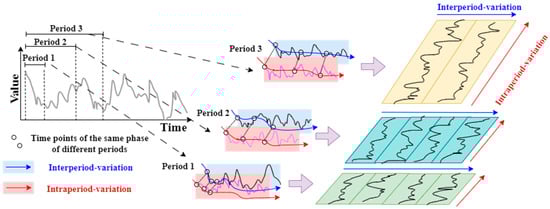
Figure 1.
Multi-periodicity and temporal 2D variation of time series.
In TimesNet, the TimesBlock is designed to integrate the aforementioned process and effectively model the two types of variations with the parameter-efficient inception block. The configurations of TimesNet will be described in detail below.
The Theory of Transformation from 1D Variation into 2D Variation
In order to capture and represent the temporal variations within and between periods consistently, it is essential to investigate the periodicities of the time series. This can be achieved by applying the Fast Fourier Transform (FFT) along the time dimension of the 1D time series, denoted as , where represents the time length and denotes the input feature dimension. The FFT computation on the time dimension allows us to identify the periodic patterns presented in the time series as follows:
where represents the strength of each frequency component in . The largest of frequencies correspond to the most significant periodic lengths in the time series. This process can be succinctly described as follows:
As illustrated in Figure 2, the original 1D time series is folded based on the selected periods. This process can be formalized as follows:
where refers to the process of appending zeros at the end of the sequence to ensure that the sequence length is divisible by . By performing the aforementioned operations, we obtain a set of 2D tensors , where each corresponds to the 2D temporal variations dominated by the period .
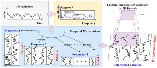
Figure 2.
A univariate example to illustrate 2D structure in time series.
TimesBlock
The architecture of TimesNet is shown in Figure 3. For the -th layer of the TimesBlock, the input is , and can be extracted 2D temporal variations by using 2D convolutional processing. The process can be formalized as:
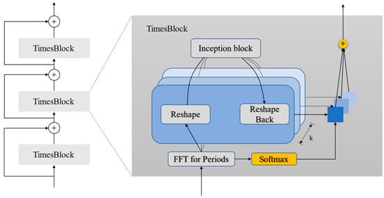
Figure 3.
Overall structure of the TimesNet.
The whole process of TimesBlock for capturing temporal 2D variations of time series will be elaborated in detail, which consists of the following four sub-processes:
- (1)
- Transforming 1D time series to 2D tensor.
First, the 1D temporal features of the input are extracted for periods and transformed into a 2D tensor to represent the 2D temporal changes. Following the process described in the previous discuss, the formulas can be rewritten as:
- (2)
- Capturing 2D temporal variations representation.
For the 2D tensors , which possess 2D locality, we can utilize 2D convolutions to extract information. Here, we adopt the classical Inception model.
- (3)
- Transforming 2D tensor to 1D Space.
After capturing the temporal features, we convert them back to 1D space for information aggregation.
where , represents the removal of the zeros added during the operation in step (1).
- (4)
- Adaptive aggregation.
Similar to the design in Autoformer [28], the adaptive fusion is performed by taking the weighted sum of the obtained 1D representations based on their corresponding frequency values, resulting in the final output.
TimesBlock is capable of simultaneously capturing fine-grained and multi-scale temporal 2D patterns [29]. As a result, compared to directly extracting features from 1D time series, TimesNet achieves more efficient representation learning.
2.1.2. Temporal Convolutional Network
The TCN captures the temporal features and long-term dependencies of load data by using a unique architecture with causal convolution, dilated convolution, and residual connections. Each module in TCN has the following detailed descriptions:
- (1)
- Causal convolution
TCN adopts a unique causal convolution that ensures the causal relationship of the input sequence, meaning the network’s output is only dependent on past inputs. Taking Figure 4a as an example, the output at time is only related to previous inputs , and it is independent of future inputs . As a result, it can avoid the leakage of future data, making causal convolution more suitable for capturing the intrinsic patterns in power load data.
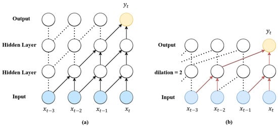
Figure 4.
(a) Causal convolution; (b) dilated convolution.
- (2)
- Dilated convolution
Although the stacking of causal convolutional layers can increase the receptive field of the network, the number layers of causal convolution will be increased for a long sequence and then lead to the gradient vanishing and exploding. The TCN introduces dilated convolutions to exponentially increase the receptive field of the network. Dilated convolution involves sampling the input of the upper layer with a certain interval, and the dilation rate grows exponentially with a base of 2 [34]. In this way, it can achieve a large receptive field with fewer layers of the network. The computation formula for dilated convolution is as follows:
where is the dilation rate, is the filter size, and represents the convolution of the past state. Thus, the dilated convolution significantly reduces the network complexity and improves computational efficiency.
- (3)
- Residual block
To ensure the stability of TCN with a large number of layers, residual connections were introduced between two dilated convolutional layers [35]. The advantage is that it avoids the loss of too much information during the feature extraction process of TCN. The residual module is mainly composed of two dilated causal convolutions, batch normalization, dropout, ReLU activation function, and other modules, as shown in Figure 5a. Additionally, the residual block adopts a convolution to ensure the same dimensions of the input and output. Figure 5b illustrates a deep TCN model stacked by multiple residual blocks. Therefore, a deep TCN enables the network to look back into the past for feature extraction to obtain long-range dependencies.
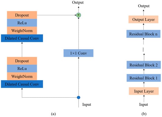
Figure 5.
(a) The structure of the TCN; (b) deep TCN.
2.2. Ensemble Framework
In order to achieve higher prediction accuracy, this paper proposes a novel hybrid framework for STLF based on TimesNet and TCN. Figure 6 shows the flow chart of the ensemble framework. The overall process of the load forecasting can be roughly divided into four steps. According to the flow chart of the proposed model, the detailed descriptions of each step are as follows:
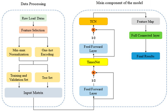
Figure 6.
Flow chart of the ensemble framework.
Step 1: Data processing. Real-world load data are usually corrupted with missing values or outliers due to malfunction of sensors or human error [35]. This will inevitably affect the prediction accuracy of the model. To overcome this issue, the following methods can be used to handle missing values or outliers. For example, missing data can be replaced with the average of the previous and next time points, or with the data from the same time point of the previous day. Afterward, the load demand and temperature will be normalized by min-max normalization and day types will be processed by one-hot encoding. Finally, the load demand and external factors are reconstructed in an input matrix.
Step 2: Feature extraction. Feature extraction is very important for achieving high accuracy of STLF. Firstly, the input matrix is fed into the feed-forward layer with residual connection to enhance its nonlinear representations. Secondly, the output will be passed through the TimesNet module to extract the dependencies within different time scales and the relationships between different time scales of the power load data. Finally, the feature matrix is processed through the feed-forward layer with a residual connection and then fed into the TCN module, leveraging its excellent time series processing capabilities to extract temporal features and long-term dependencies of the power load data. It is worth mentioning that in this study, residual connections were introduced in the feedforward process to optimize the network performance.
Step 3: Load Forecasting and Parameter Optimization. After completing the feature extraction of the power load data through the aforementioned steps, the load forecasting is achieved from the fully connected layer. Then, the model parameters are validated using the validation set. If the model shows an improvement in accuracy on the validation set, the current model parameters will be saved and the model is updated for further training. Otherwise, the model training continues until the optimal model is obtained.
Step 4: Model Evaluation. After obtaining the optimal model through Step 3, the performance of the model is verified by using the testing set. The mean absolute percentage error (MAPE) and root mean square error (RMSE) are used as evaluation indices to evaluate the performance of the proposed model.
3. Experiments Results and Analysis
To evaluate the effectiveness of the proposed model in this paper, a series of experiments will be conducted on a public dataset. Additionally, in order to highlight the advantages of the proposed model, it will be compared with other TCN-based models. The hyper-parameters of these models will be adjusted based on previous experience to achieve optimal performance. All models will be run on a PC with Inter core i7-11800H CPU and NVIDIA Tesla V100S-PCIE-32 GB GPU. In this study, the programming environment is PyTorch 1.10 and CUDA 10.2. The PyTorch is a widely used deep learning framework that offers a variety of pre-trained models, tools, and extension libraries, facilitating the development and training of deep neural network models. Additionally, the PyTorch supports efficient computations on GPUs, accelerating training processes. In the following, we will provide a detailed description of experimental settings, feature selection and preprocessing, as well as comparative analysis of experimental results.
3.1. Experimental Design
3.1.1. Data Preparation
In order to evaluate the effectiveness and generalization of the proposed model, two datasets were utilized to perform experiments. The first dataset was collected from a public dataset of ISO-NE (New England) [36], which consists of power load from 1 March 2003 to 31 December 2014 in New England of the United States. The dataset includes load demand, temperature, and day types with one-hour resolution. A total of 43,920 sets of data are selected for experiments. According to the ratio of 8:1:1, the training set consists of 35,136 data points, while the validation and testing sets contain 4392 data points. The second dataset was collected from the state grid of a region in Southern China. The time range was from 1 January 2012 to 10 February 2014 with sampling every 15 min [37]. The total dataset with 106,176 sets will divided into a training set, a validation set, and a testing set with the proportion of 8:1:1. The ISO-NE public dataset was used to analyze the feature selection and processing and compare with other benchmarking models to verify the superior performance of the proposed model, while the Southern China dataset was adopted to further exhibit the generalization of the proposed model.
3.1.2. Sliding Window Settings
The setting of the sliding window is crucial for accurate and effective data processing. The length and step size of the sliding window needs to be carefully determined to meet two aspects: capturing sufficient historical information and maintaining reasonable computational complexity [38]. Thus, after extensive optimization experiments, the length of a sliding window is 24 steps with a step size of 1. It means that each sliding window contains 24 rows of data and then all models predict the load demand of the next step through the features of the previous 24 steps.
3.1.3. Comparative Models
To validate the superior performance of the proposed model, the following models are used for comparison in this study: CNN, LSTM, TCN, TimesNet, TCN-LSTM, and TimesNet-LSTM. The hyper-parameters of all these models are adjusted appropriately based on previous experience to optimize their performances.
3.1.4. Model Evaluation Criteria
In order to evaluate the performance of the proposed model, it is convenient to use the MAPE and RMSE as evaluation indices. The smaller the values of MAPE and RMSE, the higher the prediction accuracy of the model. The formulas for MAPE and RMSE are defined as follows:
where represents the total number of prediction points, represents the true value, and represents the predicted value.
3.2. Feature Selection and Processing
Due to various external factors, power load data often exhibit fluctuations and randomness, making accurate load prediction challenging. Therefore, selecting appropriate features is crucial to improve the prediction accuracy of the model. To select suitable features as inputs for the model, an analysis of the original dataset is required. Figure 7 shows the change of load demand for 30 days in the New England region of the United States. It is evident that the changing trend of power load data exhibits a weekly pattern, with smaller fluctuations during weekdays and significantly higher load during weekends. This observation suggests that the reduced overall electricity load on weekends may be due to the shutdown of institutions such as companies and factories with high electricity consumption. Similarly, some national holidays are also likely to have a significant impact on the power load. Figure 8 depicts the profiles of power load and temperature over 6 years based on the ISO-NE dataset. It can be observed that the power load has 12 peaks and valleys, because the power demand usually reaches peaks when the temperature is very high or low. Therefore, temperature and day types have a significant impact on STLF. Considering the periodicity, randomness, trend, and external factors affecting electricity load, the experiments select five features, i.e., power load, temperature, holidays, seasons, and weekends, for load forecasting.
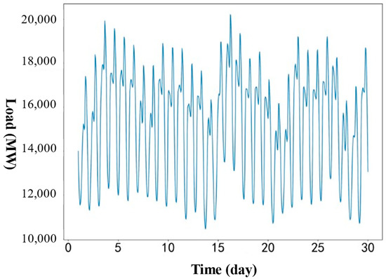
Figure 7.
Daily load profile of 30 days for ISO-NE dataset.
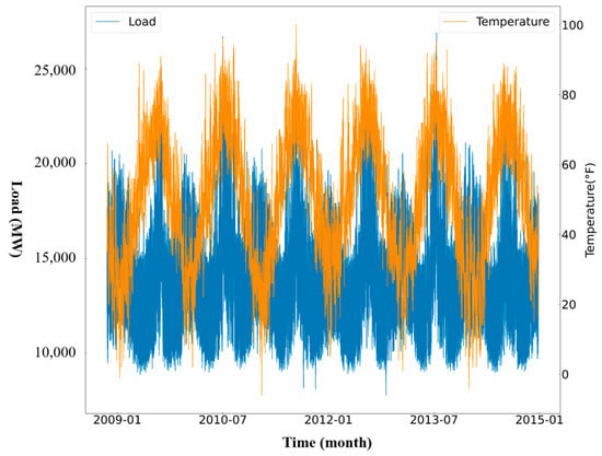
Figure 8.
Daily load and temperature profile of 6 years for ISO-NE dataset.
To improve the stability and accelerate the convergence speed of the model, we performed min-max normalization on the electricity load and temperature data. The min-max normalization scales the data to a specific range, ensuring that the feature data has a consistent scale and eliminating differences between various features, thereby enhancing the performance and stability of the model. The formula for min-max normalization is defined as follows:
where represents the entire time series, represents the normalized feature value, is the original feature value, and and are the minimum and maximum values of the feature in the dataset. Additionally, the one-hot encoding is used for holiday, weekday, weekend, and quarter. The specific processing method is shown in Table 1. After the feature selection and processing of the original load data, a feature matrix is reconstructed and then input into the ensemble framework for training the model to obtain experimental results.

Table 1.
One-hot encoding.
3.3. Comparative Analysis of Experimental Results
To validate the superiority of the proposed model, the following prediction models were selected for comparative experiments: CNN, LSTM, TCN, TimesNet, TCN-LSTM, and TimesNet-LSTM. To ensure the credibility of the results, efforts were made to keep other unrelated factors consistent, such as the selection and partitioning of training, validation, and testing sets. Additionally, based on previous experience, the hyperparameters of each model were adjusted appropriately to achieve optimal performance. Furthermore, each model was trained and tested at least five times, and the experimental results were averaged.
3.3.1. ISO-NE Dataset
Table 2 presents the experimental results of all these models based on ISO-NE dataset. For the single models, compared to CNN, the MAPE and RMSE of the LSTM and TCN are decreased by 8.8%, 11% and 10.9%, 13%, respectively. This is because power load data primarily consists of time series with strong trends, periodicities, and uncertainties. However, CNN is limited to capturing local spatial features, resulting in poor performance in time series analysis. Additionally, as widely applied models in time series processing, TCN and LSTM showed superior performances in the extraction of temporal features, and TCN achieves a 2.4% decrease in terms of MAPE compared to LSTM. This can be attributed to the ability of TCN’s convolutional operations to directly capture patterns across different time intervals, addressing the issues of gradient vanishing and exploding gradients commonly encountered in LSTM when modeling long-term dependencies in time series. Furthermore, as a newly proposed model, TimesNet exhibits exceptional performance with a significant reduction of 23.4% and 14.6% in terms of MAPE and RMSE compared to TCN. This is because TimesNet models the transformation of 1D time series into 2D variations, enabling an in-depth mining of the dependencies within different time scales and relationships between different times scales. By employing the renowned Inception block for extracting complex temporal changes of the transformed 2D tensors through 2D convolutions, TimesNet achieves a higher prediction accuracy compared to traditional RNN-based models.
Table 2.
The evaluation metrics for load forecasting of each model for ISO-NE dataset.
For hybrid models, compared to their constituent single models, the MAPE and RMSE values of the hybrid models show varying degrees of improvement. For example, compared to TCN and LSTM, the TCN-LSTM hybrid model achieves a decrease of 13.6%, 15.6% and 8.1%, 10.4% in terms of MAPE and RMSE, respectively. Furthermore, compared to LSTM and TimesNet, the TimesNet-LSTM hybrid model achieves a decrease of 28.9%, 4.8% and 19.7%, 3.4% in terms of MAPE and RMSE, respectively. These results demonstrate the advantages of hybrid models used in the field of power load forecasting. Hybrid models leverage the strengths of their individual modules, allowing for the utilization of their individual characteristics. It is obvious that, combing the powerful capabilities of TimesNet and TCN, the TimesNet-TCN hybrid model achieves the best performance in this study. Compared to other hybrid models, the proposed model achieves significant decreases in terms of MAPE and RMSE. For example, compared to the TCN-LSTM model, the proposed model achieves a decrease of 32.9% in MAPE and 15.8% in RMSE. Furthermore, compared to TimesNet-LSTM model, the proposed model achieves a decrease of 20.3% in MAPE and 6.1% in RMSE. These results can be attributed to the powerful capabilities of TimesNet and TCN, utilizing causal convolutions and dilated convolutions, to capture the temporal features and long-term dependencies of time series data in a more global manner. It should point out that the proposed model requires more running time due to the multiple convolutional layers in the Inception block of TimesNet. However, the running time of the proposed model only increases by 1.2% compared to that of the TimesNet model. In the real application for massive data, the costing time of the proposed model is acceptable when considering the improvement of the prediction accuracy.
In order to visually demonstrate the superiority of the proposed model, Figure 9 presents the load prediction curves of all the models and the actual load data for 24 h. One can find that the predicted load values of all the models can roughly fit the changing trend of the actual load data. However, the proposed model shows a stronger fitting capability to the actual load data compared to other comparative models, especially during the peak or valley region.
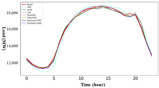
Figure 9.
Load forecasting profiles of all models for 24 h based on ISO-NE dataset.
3.3.2. Southern China Dataset
Table 3 shows the experimental results of all these models based on the Southern China dataset. Compared with Table 2, the values of MAPE of these models are larger than those of the ISO-NE dataset while the values of RMSE are smaller than those of the ISO-NE dataset. It is because the time resolution of the Southern China dataset is only 15 min and the length of the sliding window with 24 steps only covers a time span of 6 h. In this case, the multi-periodicity of load data cannot be reflected obviously compared to the ISO-NE dataset and the overall deviation of the predicted load values will also be significantly increased accordingly. Compared to the single models, such as CNN, LSTM, TCN, and TimesNet, the MAPE of the proposed model is decreased by 40.2%, 30.7%, 29.9%, and 17.6%, respectively. At the same time, the RMSE of the proposed model is also decreased by 54.6%, 50%, 49.2%, and 35.5%, respectively. For hybrid models, the MAPE and RMSE of the proposed model are decreased by 21.8% and 37.8% compared to those of the TCN-LSTM hybrid model. Moreover, compared to the TimesNet-LSTM hybrid model, the proposed model achieves a decrease of 10.3% in MAPE and 11% in RMSE. In addition, Figure 10 shows the load prediction curves of all the models for 6 h based on the Southern China dataset. One can see that although the predicted load values of all these models roughly fit the changing profile of actual load, the predicted load of the proposed model is the most consistent with the actual load. These results further demonstrate that the TimesNet network can capture the temporal patterns from the load data with multi-periodicities compared to other single models. Furthermore, it is necessary to integrate the TCN into the TimesNet-based framework to enhance the ability to capture the temporal features and long-range dependencies among the time points of the load series. Therefore, the proposed model has superior performance and a strong generalization capability in STLF.
Table 3.
The evaluation metrics for load forecasting of each model for Southern China dataset.
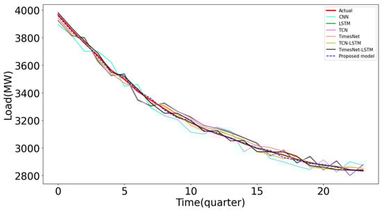
Figure 10.
Load forecasting profiles of all models for 6 h based on Southern China dataset.
3.3.3. Comparison of the Proposed Model with Other Reported Models
With the development of smart grid, it is increasingly easy to collect power load data and other external factors. More and more works have been devoted to investigating STLF in recent years. The predicted results of some papers reported recently were selected to compare with that of the proposed model for the same ISO-NE dataset, as shown in Table 4. One can see that the proposed model outperforms other reported models in terms of MAPE. For example, Ref. [32] used multiple ResNets to improve the prediction accuracy of STLF. However, the ResNet is a variant of CNN and cannot effectively capture temporal features and long-range dependences of the load data. Ref. [33] proposed a multivariate TCN model to parallelly process input variables to improve the prediction accuracy. Although the proposed model can capture the temporal features and long-range dependencies of load data, it cannot extract the intraperiod- and interperiod-variations of multi-periodicities. Refs. [29,31] were developed to fully capture the temporal and spatial features of load data. Although they have achieved higher accuracy of STLF, these works did not exploit the intricate temporal variations of load series. Therefore, we can conclude that the proposed model in this study can not only extract the local correlations and long-range dependencies of the load data, but also capture the temporal patterns from the different periods of the load data.
Table 4.
Performance comparison of some reported models based on ISO-NE dataset.
4. Conclusions
This paper proposed a novel hybrid model for STLF based on TimesNet, TCN and feed-forward layer with a residual connection. Firstly, TimesNet transformed the 1D time series into a set of 2D tensors based on multiple periods, presenting a 2D temporal variation. Then, through the parameter-efficient inception block, complex time variations were extracted, including the dependencies within different time scales and the relationships between different time scales. Secondly, TCN introduced causal convolutions, dilated convolutions, and residual connections to further extract the temporal features and long-term dependencies of the time series in a global manner. Thirdly, the feed-forward layer with residual connection was located before the TimesNet and TCN modules to enhance the nonlinear representations of the input matrix. Finally, the task of STLF is accomplished through fully connected layers.
The proposed model was evaluated by ISO-NE and Southern China datasets. Compared to other models, the experimental results demonstrated that the proposed model reduced the MPAE by 20% to 43% and the RMSE by 6% to 32.8% for the ISO-NE dataset, and the MAPE by 10% to 40% and the RMSE by 11% to 54.6% for the Southern China dataset. Overall, the novel framework developed in this study greatly improved the prediction accuracy and had strong generalization in STLF. Thus, the proposed model can contribute to the stable operation of the power systems, thereby improving economic and social benefits.
There is still an amount of work to be performed as future work. The TimesNet costs a large amount of computational time due to its ability to extract temporal features in a 2D space. Although the incorporation of the TCN indeed enhances the feature extraction capabilities and improves the accuracy of STLF, it does not reduce the computational time of the TimesNet. In future work, we aim to exploit improvements within the TimesNet framework to address the computational efficiency. Moreover, we will further optimize the extraction capabilities of features of the model to achieve higher prediction accuracy.
Author Contributions
Conceptualization, C.Z. and J.W.; methodology, C.Z.; software, M.L.; validation, C.Z., J.W. and M.L.; formal analysis, C.Z. and S.D.; investigation, M.L. and S.D.; resources, Q.W.; data curation, C.Z. and M.L.; writing—original draft preparation, C.Z.; writing—review and editing, M.L.; visualization, J.W.; supervision, Q.W.; project administration, M.L. and S.D.; funding acquisition, M.L. and S.D. All authors have read and agreed to the published version of the manuscript.
Funding
This research was funded by the National Natural Science Foundation of China under Grant 61865011 and Grant 62065012, and in part by the Natural Science Foundation of Jiangxi Province of China under Grant 20212BAB202031, and in part by the Interdisciplinary Innovation Fund of Natural Science, Nanchang University under Grant 9167-28220007-YB2111, and in part by the National College Students’ Innovation and Entrepreneurship Training Program under Grant 2022CX260.
Data Availability Statement
Data available in a publicly accessible repository that does not issue DOIs Publicly available datasets were analyzed in this study. These data can be found here: https://www.iso-ne.com/isoexpress/web/reports/load-and-demand (accessed on 7 June 2022) and https://github.com/keatoncu/Southern-China-Dataset (accessed on 7 June 2022).
Conflicts of Interest
The authors declare that they have no known competing interests or personal relationships that could have influenced the work reported in this paper.
Nomenclature
| Abbreviations | parameters | ||
| STLF | short-term power load forecasting | T | time length |
| TCN | temporal convolutional network | input feature dimension | |
| LSTM | long short-term memory | A | strength of each frequency |
| ANN | artificial neural networks | frequencies | |
| SVM | support vector machines | periodic lengths | |
| CNN | convolutional neural network | input at time t | |
| RNN | recurrent neural network | d | dilation rate |
| FFT | fast fourier transform | k | filter size |
| MAPE | mean absolute percentage error | true value | |
| RMSE | root mean square error | predicted value |
References
- Kong, W.; Dong, Z.Y.; Jia, Y.; Hill, D.J.; Xu, Y.; Zhang, Y. Short-term residential load forecasting based on LSTM recurrent neural network. IEEE Trans. Smart Grid 2019, 10, 841–851. [Google Scholar] [CrossRef]
- Hafeez, G.; Alimgeer, K.S.; Khan, I. Electric load forecasting based on deep learning and optimized by heuristic algorithm in smart grid. Appl. Energy 2020, 269, 114915. [Google Scholar] [CrossRef]
- Liu, J.; Li, Y. Study on environment-concerned short-term load forecasting model for wind power based on feature extraction and tree regression. J. Clean. Prod. 2020, 264, 121505. [Google Scholar] [CrossRef]
- Makrygiorgou, J.J.; Karavas, C.S.; Dikaiakos, C.; Moraitis, I.P. The electricity market in Greece: Current status, identified challenges, and arranged reforms. Sustainability 2023, 15, 3767. [Google Scholar] [CrossRef]
- Xiao, L.; Shao, W.; Liang, T.; Wang, C. A combined model based on multiple seasonal patterns and modified firefly algorithm for electrical load forecasting. Appl. Energy 2016, 167, 135–153. [Google Scholar] [CrossRef]
- Zhang, L.; Harnefors, L.; Nee, H.-P. Power-synchronization control of grid-connected voltage-source converters. IEEE Trans. Power Syst. 2010, 25, 809–820. [Google Scholar] [CrossRef]
- Hong, T.; Fan, S. Probabilistic electric load forecasting: A tutorial review. Int. J. Forecast. 2016, 32, 914–938. [Google Scholar] [CrossRef]
- Wang, H.; Ruan, J.; Wang, G.; Zhou, B.; Liu, Y.; Fu, X.; Peng, J. Deep learning-based interval state estimation of AC smart grids against sparse cyber attacks. IEEE Trans. Ind. Inform. 2018, 14, 4766–4778. [Google Scholar] [CrossRef]
- Boglou, V.; Karavas, C.; Karlis, A.; Arvanitis, K.G.; Palaiologou, I. An optimal distributed RES sizing strategy in hybrid low voltage networks focused on EVs’ integration. IEEE Access 2023, 11, 16250–16270. [Google Scholar] [CrossRef]
- Boglou, V.; Karavas, C.-S.; Karlis, A.; Arvanitis, K. An intelligent decentralized energy management strategy for the optimal electric vehicles’ charging in low-voltage islanded microgrids. Int. J. Energy Res. 2022, 46, 2988–3016. [Google Scholar] [CrossRef]
- Karavas, C.-S.G.; Plakas, K.A.; Krommydas, K.F.; Kurashvili, A.S.; Dikaiakos, C.N.; Papaioannou, G.P. A review of wide-area monitoring and damping control systems in Europe. In Proceedings of the 2021 IEEE Madrid PowerTech, Madrid, Spain, 28 June–2 July 2021; pp. 1–6. [Google Scholar]
- Song, K.-B.; Baek, Y.-S.; Hong, D.H.; Jang, G. Short-term load forecasting for the holidays using fuzzy linear regression method. IEEE Trans. Power Syst. 2005, 20, 96–101. [Google Scholar] [CrossRef]
- Zhang, J.; Wei, Y.-M.; Li, D.; Tan, Z.; Zhou, J. Short term electricity load forecasting using a hybrid model. Energy 2018, 158, 774–781. [Google Scholar] [CrossRef]
- Deng, Z.; Wang, B.; Xu, Y.; Xu, T.; Liu, C.; Zhu, Z. Multi-scale convolutional neural network with time-cognition for multi-step short-term load forecasting. IEEE Access 2019, 7, 88058–88071. [Google Scholar] [CrossRef]
- Ling, S.H.; Leung, F.H.F.; Lam, H.K.; Lee, Y.-S.; Tam, P.K.S. A novel genetic-algorithm-based neural network for short-term load forecasting. IEEE Trans. Ind. Electron. 2003, 50, 793–799. [Google Scholar] [CrossRef]
- Li, W.; Yang, X.; Li, H.; Su, L. Hybrid forecasting approach based on GRNN neural network and SVR machine for electricity demand forecasting. Energies 2017, 10, 44. [Google Scholar] [CrossRef]
- Aprillia, H.; Yang, H.-T.; Huang, C.-M. Statistical load forecasting using optimal quantile regression random forest and risk assessment index. IEEE Trans. Smart Grid 2021, 12, 1467–1480. [Google Scholar] [CrossRef]
- Soon, F.C.; Khaw, H.Y.; Chuah, J.H.; Kanesan, J. Hyper-parameters optimization of deep CNN architecture for vehicle logo recognition. IET Intell. Transp. Syst. 2018, 12, 939–946. [Google Scholar] [CrossRef]
- Aly, H.H.H. A proposed intelligent short-term load forecasting hybrid models of ANN, WNN and KF based on clustering techniques for smart grid. Electr. Power Syst. Res. 2020, 182, 106191. [Google Scholar] [CrossRef]
- Deng, L.; Yu, D. Deep learning: Methods and applications. Found. Trends® Signal Process. 2014, 7, 197–387. [Google Scholar] [CrossRef]
- Eskandari, H.; Imani, M.; Moghaddam, M.P. Convolutional and recurrent neural network based model for short-term load forecasting. Electr. Power Syst. Res. 2021, 195, 107173. [Google Scholar] [CrossRef]
- Sheng, Z.; Wang, H.; Chen, G.; Zhou, B.; Sun, J. Convolutional residual network to short-term load forecasting. Appl. Intell. 2021, 51, 2485–2499. [Google Scholar] [CrossRef]
- Bai, S.; Kolter, J.Z.; Koltun, V. An empirical evaluation of generic convolutional and recurrent networks for sequence modeling. arXiv 2018, arXiv:1803.01271. [Google Scholar]
- Lara-Benítez, P.; Carranza-García, M.; Luna-Romera, J.M.; Riquelme, J.C. Temporal convolutional networks applied to energy-related time series forecasting. Appl. Sci. 2020, 10, 2322. [Google Scholar] [CrossRef]
- LeCun, Y.; Bengio, Y.; Hinton, G. Deep learning. Nature 2015, 521, 436–444. [Google Scholar] [CrossRef] [PubMed]
- Chung, J.; Gulcehre, C.; Cho, K.; Bengio, Y. Empirical evaluation of gated recurrent neural networks on sequence modeling. arXiv 2014, arXiv:1412.3555. [Google Scholar]
- Vaswani, A.; Shazeer, N.; Parmar, N.; Uszkoreit, J.; Jones, L.; Gomez, A.N.; Kaiser, L.; Polosukhin, I. Attention is all you need. arXiv 2017, arXiv:1706.03762. [Google Scholar]
- Wu, H.; Xu, J.; Wang, J.; Long, M. Autoformer: Decomposition transformers with auto-correlation for long-term series forecasting. In Proceedings of the Advances in Neural Information Processing Systems, Online, 6–14 December 2021; Volume 34, pp. 22419–22430. [Google Scholar]
- Wu, H.; Hu, T.; Liu, Y.; Zhou, H.; Wang, J.; Long, M. TimesNet: Temporal 2D-variation modeling for general time series analysis. arXiv 2023, arXiv:2210.02186. [Google Scholar]
- Kim, T.-Y.; Cho, S.-B. Predicting residential energy consumption using CNN-LSTM neural networks. Energy 2019, 182, 72–81. [Google Scholar] [CrossRef]
- Rafi, S.H.; Nahid-Al-Masood; Deeba, S.R.; Hossain, E. A short-term load forecasting method using integrated CNN and LSTM network. IEEE Access 2021, 9, 32436–32448. [Google Scholar] [CrossRef]
- Cai, W.; Zhang, W.; Hu, X.; Liu, Y. A hybrid information model based on long short-term memory network for tool condition monitoring. J. Intell. Manuf. 2020, 31, 1497–1510. [Google Scholar] [CrossRef]
- He, K.; Zhang, X.; Ren, S.; Sun, J. Deep residual learning for image recognition. In Proceedings of the IEEE Conference on Computer Vision and Pattern Recognition (CVPR), Las Vegas, NV, USA, 27–30 June 2016; pp. 770–778. [Google Scholar]
- Lea, C.; Vidal, R.; Reiter, A.; Hager, G.D. Temporal convolutional networks: A unified approach to action segmentation. In Proceedings of the Computer Vision—ECCV 2016 Workshops, Amsterdam, The Netherlands, 8–10, 15–16 October 2016; pp. 47–54. [Google Scholar]
- Hua, H.; Liu, M.; Li, Y.; Deng, S.; Wang, Q. An ensemble framework for short-term load forecasting based on parallel CNN and GRU with improved ResNet. Electr. Power Syst. Res. 2023, 216, 109057. [Google Scholar] [CrossRef]
- ISO New England-Energy, Load, and Demand Reports. Available online: https://www.iso-ne.com/isoexpress/web/reports/load-and-demand (accessed on 7 June 2022).
- Southern China Data Set. Available online: https://github.com/keatoncu/Southern-China-Dataset (accessed on 7 June 2022).
- Liu, M.; Sun, X.; Wang, Q.; Deng, S. Short-term load forecasting using EMD with feature selection and TCN-based deep learning model. Energies 2022, 15, 7170. [Google Scholar] [CrossRef]
- Kondaiah, V.Y.; Saravanan, B. A modified deep residual network for short-term load forecasting. Front. Energy Res. 2022, 10, 1038819. [Google Scholar] [CrossRef]
- Wan, R.; Mei, S.; Wang, J.; Liu, M.; Yang, F. Multivariate temporal convolutional network: A deep neural networks approach for multivariate time series forecasting. Electronics 2019, 8, 876. [Google Scholar] [CrossRef]
Disclaimer/Publisher’s Note: The statements, opinions and data contained in all publications are solely those of the individual author(s) and contributor(s) and not of MDPI and/or the editor(s). MDPI and/or the editor(s) disclaim responsibility for any injury to people or property resulting from any ideas, methods, instructions or products referred to in the content. |
© 2023 by the authors. Licensee MDPI, Basel, Switzerland. This article is an open access article distributed under the terms and conditions of the Creative Commons Attribution (CC BY) license (https://creativecommons.org/licenses/by/4.0/).