Abstract
Achieving a good level of resilience to extreme events caused by severe weather conditions is a major target for operators in modern power systems due to the increasing frequency and intensity of extreme weather phenomena. Moreover, regulatory authorities are pushing transmission and distribution operators to prepare resilience plans suitably supported by Cost–Benefit Analyses (CBAs). In this context, this paper proposes a CBA framework based on Optimization via Simulation (OvS) for the selection of the optimal portfolio of resilience enhancement measures. Starting from a comprehensive set of candidate grid hardening and operational measures, the optimal mix is identified by applying a novel two-step procedure based on an efficient application of the generalized pattern search heuristic technique. Risk indicators for the CBA are quantified, accounting for probabilistic models of climate changes. Moreover, the potential cascading outages due to multiple component failures provoked by extreme events are simulated on selected scenarios. The examples carried out on an IEEE test system show the effectiveness of the approach in identifying the best portfolio of resilience enhancement measures depending on climate change projections and costs of the measures, while the application to the model of a large portion of the Italian EHV transmission system demonstrates the practicability of the approach in real-world studies to support operators in different power system management phases, from planning to operation.
1. Introduction
The topic of resilience has entered the agenda of transmission and distribution system operators worldwide with the aim to improve power supply performances in the case of extreme events, such as those caused by severe weather conditions [1]. Resilience indeed is defined by CIGRE as “the ability to limit the extent, severity and duration of system degradation following an extreme event” [2]. System operators are often urged by regulatory authorities to prepare resilience plans, and they call for tools supporting them in performing a Cost–Benefit Analyses (CBA) to prioritize the interventions in their resilience plans [3].
A useful classification of resilience enhancement measures (also for the sequel of the paper) distinguishes the “passive” measures, aimed at hardening the system infrastructure to make it less vulnerable to threats, from the “active” measures, aimed at achieving smarter system operation. The hardening of tower supports is an example of the former type of measure, while generation redispatching is an example of the latter.
Research is very active in developing methodologies and tools to help operators attain this goal.
In [4], the benefits of several measures against windstorms are assessed via sequential Monte Carlo (MC) simulations for the UK system. The risk-based resilience assessment methodology in [5] relies on detailed analytical models of component vulnerabilities, countermeasures, and threats, and it accounts for potential cascading failures. It can be used to quantify the benefits in terms of reduced risk of loss of load for both hardening and operational measures against extreme events, in particular wet snow events.
The objective of enhancing grid resilience at minimum costs is studied in [6,7,8,9,10,11,12]. Notably, the optimization framework based on conditional value at risk in [6] is aimed at re-designing distribution substations with minimum cost and limited risk exposure to generic severe events. In [7], investment portfolios that offer the highest resilience enhancements against potential risks caused by generic natural hazards are optimized using a sequential MC simulation. Reference [7] focuses on the selection of the most resilience-oriented investments among a predefined set of hardening alternatives without assessing the potential of measures at the operation stage. Reference [10] proposes a decision framework to minimize investments in the hardening and selective expansion of power and gas distribution networks and operation costs considering the feasibility of the solutions under natural disasters: as in [7], the focus is on hardening solutions.
In most papers [4,6,7], the environmental events are simulated as “possible realizations” of a hazard based on historical data; however, climate changes (CCs) may affect the features (frequency, duration, severity, and extension) of the hazard itself over the typical multi-year horizons of grid planning. In [8], the authors evaluate some scenarios to account for the effects of potential future high temperatures due to climate evolution on the usable power of generating plants, but climate evolution (in terms of water availability and maximum temperatures) is preliminarily accounted for, considering only a limited set of possible future scenarios.
Reference [9] presents a method for modeling the value of resilience that is flexible and scalable across multiple types of models. The article describes a framework for incorporating duration-dependent customer damage functions into planning and operational models.
In [11], the authors present a two-level optimization algorithm for a resilience-oriented planning of both transmission and distribution grids, considering only investment costs without operational measures. In addition, in this case hazard scenarios are modeled based on historical data series concerning past events.
In [12], the hazard scenarios are modeled considering historical data about the paths followed by hurricanes in the same area in the past, without considering the potential modification of frequency and intensity of the phenomena due to climate changes.
Many references [6,7,11,12] do not evaluate the potential cascading failures following the disturbances induced by the threat; however, in recent years more and more attention has been devoted to this topic in resilience studies [13,14].
To summarize, the main limitations highlighted in the current methodologies for resilience assessment and enhancement are the following: (1) most of the methods quantify the costs and the benefits related to a limited set of measures identified “a priori” on a qualitative basis (e.g., operators’ experience), but they do not directly identify the most cost-effective mix of both passive and active measures; (2) analyses are performed neglecting (or considering in a simplified way) the impact of CCs, even if the lifetime of power infrastructures may span over several tens of years in which CCs may be relevant: in many cases only historical data are used to probabilistically characterize the hazard; (3) the impact of multiple contingencies caused by threats is generally assessed with Optimal Power Flow (OPF) tools without considering the actual response of the power system protection, control, and defense systems, which can actually lead to cascade tripping and thus to extensive customer disconnections.
To address the above gaps, the innovative aspects of this paper are as follows: (1) the general framework for resilience optimization that identifies the most cost-effective portfolio of hardening and operational measures to be deployed over different phases of power system management, from long-term planning to operation: the framework is based on Optimization via Simulation (OvS) and can be applied to different threats; it should be mentioned that previous methods proposed by the authors, e.g., [4,7], were limited to evaluating the benefits and costs related to predefined solutions or, at most, to optimizing a combination of a limited set of predefined interventions; (2) the integration of the probabilistic modeling of CC effects in the decision-making framework; (3) the exploitation of a cascading failure simulator to assess the actual response of power systems to multiple contingencies; (4) the application of an efficient solution algorithm, based on a generalized pattern search, to also optimize the resilience for realistic grids with hundreds of nodes.
The paper is organized as follows: Section 2 presents the rationale of the CBA on the basis of the proposed decision-making framework. Section 3 describes the formulation of the optimization problem and the solution algorithm. Section 4 and Section 5 present the application results on a test system and on a large portion of a real power system, respectively. Some conclusions are drawn in Section 6.
2. Problem Formulation
This section presents the rationale of the decision-making framework and the mathematical formulation of the underlying optimization problem.
2.1. Overview
Many definitions of resilience have been elaborated on in the last decades by regulating and standardizing entities. The definition of resilience adopted in the present paper is the one proposed by the CIGRE Working Group C4.47 [2] and recalled in the Introduction.
Resilience enhancement can be addressed by implementing passive measures such as asset hardening to make the infrastructure more robust to weather threats. However, active operational measures, such as the redispatch of conventional generation or the activation of emergency generation, can also be effective in preventing disturbances or in speeding up the restoration process, respectively. Resilience planning, aimed at selecting the portfolio of measures that assures the best balance between costs of interventions and benefits for resilience out of a possibly wide set of passive and active candidate measures, is quite more challenging than simply assessing predefined solutions; thus, innovative methodologies are needed.
In fact, passive measures are decided in the planning stage in order to be available at the target time horizon (months or years later), but operational measures are activated in the operational planning or operation stages, i.e., just before the critical situation or while it is unfolding.
Moreover, for the analysis of different threats, in addition to the threats’ models themselves, specific vulnerability models (either statistical or analytical, and physics-inspired) of grid components are needed, as well as those of the resilience enhancement measures. The latter can be either threat-specific (e.g., antitorsional devices against wet snow accretion on overhead lines) or generic (e.g., load shedding). The resulting optimization problem is mixed-integer, non-linear, and time-dependent (dynamic); therefore, it is computationally very challenging.
2.2. Cost–Benefit Analysis of Resilience Enhancement Measures
A CBA is a general approach used to assess and rank the convenience of planned interventions such as new lines [15,16]. In the resilience context, it can be applied to evaluate projects such as the installation of antitorsional devices to prevent wet snow accretion on overhead line conductors. Operational measures can be alternative or complementary to hardening; therefore, they should be accounted for in a CBA as well.
The basic concept of a CBA is to compare the costs and benefits of an intervention. A hardening intervention is characterized by both investment costs, e.g., infrastructure construction and equipment procurement, and by operation and maintenance costs, e.g., the maintenance of the hardened asset over its service life. Active measures may require investment costs as well, e.g., the purchase of dedicated emergency generators, the design and installation of defense schemes, the retrofitting needed to enable resources such as distributed generation to provide resilience-related services such as black start and electrical island control, etc. Operational costs are associated with preventive (decided in the operational planning stage) or corrective (decided in real time) activations in the case of expected or ongoing critical situations. Some examples are the costs for conventional generation redispatch, emergency generation fuel, etc. Maintenance costs also apply to dedicated assets managed by grid operators, such as emergency generators. In the sequel of this paper, the costs considered for active measures will be limited to preventive and corrective activations, without the loss of generality for the overall CBA approach.
The benefits of the interventions can be defined as the reduction in the costs incurred by “insufficient” resilience, i.e., in the case of events leading to power supply and/or infrastructure disruption:
- energy not served to customers;
- repair of damaged infrastructure (components and personnel costs).
When the costs of measures for resilience enhancement rise, those due to system disturbances in the case of extreme events decrease, and vice versa. A CBA approach can be used to compare different hardening solutions with each other or with respect to active solutions but also to compare different preventive or corrective solutions for a given grid-hardening configuration.
As resilience assessment regards the long-term performances of the system subject to rare events, the evaluation of the potential benefits calls for the analysis of power system response to possible events under different initial states over a multi-year period. For any hour of the time period (therefore for any state of the electrical system under consideration), the relevant quantities must be evaluated, i.e., the expected costs of the energy not served, of the repair actions, of the implementation of corrective actions, and of the preventive actions, which may or may not depend on the specific state of the power system.
2.3. Mathematical Formulation and Indicators
The mathematical formulation considers all of the above aspects. In general, for each hour h, a configuration and state of the power system are defined by the following:
- A specific topological hardening configuration with respect to the initial available components (e.g., corresponds to the set of initially existent components). The set of potential topological hardenings is Ω.
- A specific system state Xh at hour h characterized in terms of power system operating conditions (i.e., components in service, load, and generation patterns) and in terms of a specific threat scenario.
For each hour h, a set of critical contingencies (j = 1, …, Nctg,h) is also identified. To solve the potential problems in the system’s capability to supply energy in the case of these contingencies, it is possible to search for a set of preventive measures (which change the system state from Xh to Xh′, thus reducing the contingency impact on the system) and Nctg,h sets of corrective measures . In the case that no corrective and preventive actions are considered, sets and are equal to the null set (Ø). In the case of no preventive actions, system state Xh′ coincides with state Xh.
For each hour h, the economic benefit associated with the implementation of resilience measures is defined as the reduction in repair and ENS costs with respect to the initial state with no measures deployed. The net benefit Q is defined as the difference between the economic benefit and the costs for the implementation of corrective and preventive actions on a system state potentially subject to topological hardenings of set and to preventive and corrective actions :
where BENEFITs are expressed as in Equation (2)
COSTs are given by Equation (3):
and
- and are the probability of occurrence of contingency j in the initial state of the system Xh (with no measures deployed) and the probability of the same contingency j after the deployment of possible hardening measures and of the potential preventive measures that modify the system state from to , respectively.
- and are the energy not served to customers due to contingency j applied to initial state and to state , respectively, obtained after a preventive change of state also considering corrective measures which limit the contingency impact.
- is the cost to implement preventive active measures to change the system state from to in order to improve the system response to the set of contingencies which are anticipated as “critical” for state Xh by a screening method (see Section 3.1.2).
- is the cost for corrective measures aimed at limiting the impact of contingency j: it depends on hardening solutions and on the system state Xh potentially modified to by preventive measures . Recall that system state coincides with when no preventive actions are deployed.
- It is assumed that corrective actions do not affect the repair costs because they are deployed after the threat has affected the infrastructure.
- and are the cost for the repair of the infrastructure after the occurrence of contingency j in states and , respectively: this cost depends on the system state and on the system hardening but also on active (preventive and corrective) measures deployed to reduce the impact of the contingency itself.
- CENS is the unitary Cost of the Energy Not Served and it corresponds to the VOLL (Value of Lost Load): the VOLL values to be used in the CBAs of system operators are typically provided by regulating authorities.
All the costs and the monetary benefits mentioned in the above formulas are actualized by applying an average discount rate r over the T hours of the study interval composed by Ty = T/8760 years.
The total costs and benefits for the deployment of active and passive measures over the T hours of the time horizon of the analysis are given in (4).
where represents the cost of implement the hardening solution . In particular, .
In order to define resilience-informed metrics for the CBA, it is necessary to actualize the costs and the benefits considering the discount rate r over all the Ty years according to the formulas in Equation (5) showing the actualization of benefits and costs on a yearly basis, in line with the indications provided in the Italian context for the execution of CBAs.
where and are the annual benefit and cost for the y-th year of analysis, respectively, i.e., the sum of terms in Equations (2) and (3) over all the hours of the y-th year, and y0 is the initial year of the analysis.
Two important indicators for the CBA to detect the optimal mix of measures are the following:
- The Total Net Benefit (TNB) due to active and passive measures in Equation (6):
- The System Utility Indicator (SUI), also called Benefit-to-Cost Ratio (BCR) in ENTSO-E CBA [16], defined as the ratio between actualized benefits and actualized costs:
In coherence with the CIGRE definition of resilience and with the indicators above, the resilience level of a power system is quantified in the methodology by computing the risk of the energy not served to the customers due to multiple contingencies triggered by extreme events over the time horizon of interest. This indicator can be calculated both before and after the application of the optimally chosen countermeasures: in the latter case it is called “residual expected energy not served”, “residual EENS”. The mathematical expression of the residual EENS is given in Equation (8).
Other indicators are potentially useful to quantify power system resilience, such as the CVar and Var metrics introduced in the literature [17]. In the proposed approach, the TNB, SUI, and EENS metrics are adopted for coherence with the Italian TSO.
3. The Proposed Optimization Methodology
The present section describes the methodology exploited to select the mix of resilience measures and based on a scenario-based approach.
Figure 1 shows the overall optimization approach.
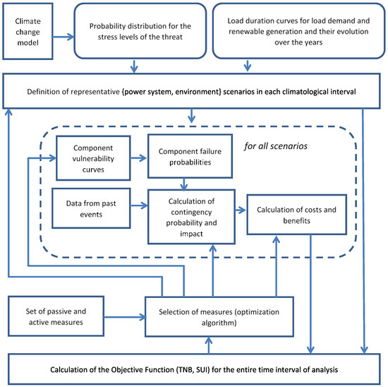
Figure 1.
Workflow of the optimization approach integrating the CBA indicators.
The subsequent subsections focus on the following aspects: (1) a scenario-based approach to integrate CBA indicators in the optimization problem, considering representative {power systems, environment} scenarios, (2) the modeling aspects concerning scenario uncertainties, (3) the formulation for the optimization of the portfolio of resilience enhancement measures via the CBA, (4) the relevant solution algorithm exploiting a direct search-based approach.
3.1. Integration of CBA Aspects in the Optimization Problem: A Scenario-Based Approach
The optimization problem must be applied to long-term scenarios characterized by the variability and uncertainty of the power system operating conditions as well as of the threat scenarios, including the effects of the climate changes.
One option would be to apply a Monte Carlo simulation; however, this approach would be very time consuming if it considers a large number of realistic generation/load and threat scenarios as well as reasonable evolutions of the climate changes for applications to large portions of real-world transmission grids. Moreover, the sampling of High-Impact, Low-Probability events in a Monte Carlo simulation requires long computational times, which can be partially limited using variance-reduction techniques such as Importance Sampling. For these reasons, a scenario-based framework with contingency enumeration is proposed, where a representative (and limited) set of scenarios is adopted to assess the interactions between the system and the environment over a long-term horizon. Probabilistic climatological models are integrated in the scenario building. The choice of a scenario-based approach is also consistent with the methodologies adopted, e.g., by the Italian TSO [18].
The proposed approach is based on the following assumptions:
- The operating points to be retained for the CBA in the optimization framework are selected considering only two stochastic variables representing plausible scenarios for load demand and renewable generation. The relevant distributions are derived from the duration curves of the total load and renewable generation available for each portion of the grid; the method used to select the representative set of operating points is described in Section 3.1.1.
- The maximum yearly stress levels associated with a threat are represented via a generalized extreme value distribution (GEV) with parameters which can be considered constant in each climatological interval of a sufficiently short duration so that the effect of climate changes can be considered negligible (e.g., 5–10 years). Thus, the Ty years of the study horizon are divided into climatological intervals ∆tp, p = 1, …, Np.
The main steps for scenario generation are as follows:
- Selection of representative {power system, environment} scenarios on the basis of the probabilistic models for CC effects and of projected duration curves.
- Definition of a set of contingencies involving the components which are more prone to fail in each scenario.
- Simulation of the impacts of contingencies.
3.1.1. Selection of Representative {Power System, Environment} Scenarios
The first step consists of the selection of a representative set of scenarios in terms of load demand and renewable generation patterns, as well as threat intensity conditions in the long run. The scenario-based approach is very suitable for optimization purposes, as it allows different levels of accuracy and time burden depending on the number of discrete values which the stochastic variables used in the problem (i.e., load demand, threat intensity, and renewable generation) can take. This aspect can be very helpful in the analysis of large power systems.
Each scenario is a specific combination of the load/generation pattern subject to a specific threat intensity. The way these discrete values for load demand, threat intensity, and renewable generation are chosen depends on the specific technique used to select the representative scenarios.
A possible way to perform the selection of the representative scenarios starts from a complete simulation of the uncertainties using a Monte Carlo simulation, followed by clustering of similar situations using techniques such as the Fast Forward Method (FFM) [19]. The selection of the N representative scenarios can benefit from the information available from the TSO (e.g., a large set of plausible operating points of the grid and realistic historical series of maximum threat intensity over the grid under study).
Regardless of the chosen aggregation method, starting from a set of operating points representative of PS operation over the years, the similarity among scenarios regarding threats and load/generation patterns can be assessed using metrics which represent the attitude of the specific operating point under specific threat conditions from the set above to initiate cascading outages in the presence of multiple contingencies, e.g., the net ability index [20], other topological indexes [21], and the profile of p.u. loadings of the branches in the grid.
Such metrics allow the identification of a limited set of {threat/load/generation} scenarios which are representative of the most frequent conditions in the annual operation of PS and which effectively aggregate scenarios that are similar in terms of exposure to threat events and response to cascading outages. Once this identification is completed, the optimization process of resilience measures can thus be performed for a subset of operating points, each one representing a typical load/generation/threat pattern which occurs over a year with significant frequency. The discussion of different metrics is out of the scope of this paper.
The number of scenarios to be retained for the CBA can be selected also considering the recommendations in [22], where ENTSO-e highlights the importance of selecting multiple scenarios to deal with the uncertainties concerning the evolution of load demand and generation capacity.
In the present paper, the scenario selection starts from the discretization of the continuous probability distributions of the load and renewable generation patterns as well as of the stress levels of the threat. In particular, based on the available data for the test system under study (i.e., the load and renewable generation duration curves and the statistics on maximum annual threat intensities over the grid), the methodology evaluates the following:
- NL discrete values of the p.u. loads and NG values of p.u. RES injections are set;
- the GEV distribution of threat intensity is discretized into Nth values for each p-th climatological interval Δtp. A specific GEV distribution is derived for each location in the grid based on historical data statistics.
In other words, the hour-based formulation in Equation (1) considering T hours is translated into a scenario-based formulation accounting for N scenarios with N < T. In particular, N represents the total number of threat/load/generation scenarios over all the climatological intervals, i.e., N = Nth × NL × NG × Np. The generic scenario is indicated with index n.
For each climatological interval, the methodology considers NL,G = NL × NG power system operating conditions (accounting for the load and generation capacity variations over the multi-year horizon) and Nth discrete intensity values of the threat. It is worth noting that in the general methodology formulation, load and renewable generation pattern and threat intensity can be modeled as correlated variables: a copula-based approach briefly recalled in Section 3.1.2 is used to quantify the probability of occurrence of each threat/load/generation scenario.
The probability distribution of threat intensity over the generic p-th climatological interval is represented as a pmf (probability mass function) over the discrete threat values, whose probabilities PTh(th, Δtp) depend on both the threat value and the climate change interval.
Given each threat value th, the conditional probabilities of the NL,G system operating conditions st associated with each climatological interval ∆tp are mutually exclusive and exhaustive, i.e.,
The (hourly) probability of component failure for each threat scenario is assessed by evaluating the vulnerability curves of the components at a variable stress value equal to th (for each threat scenario). These probabilities can also be very high, but, considering that extreme events occur only in a few hours during the year, these values are also consistent with the annual component failure rate for the same threat. These probabilities are used to calculate the probabilities of contingencies needed to evaluate the benefits of active (corrective and preventive) measures on an hourly basis.
Under these hypotheses, the total benefits and costs of the CBA can be expressed in terms of scenarios as in Equation (10), instead of a sum over hours as in Equations (4), where the lowercase variables x, , , and represent the discretizations over the n = 1,…, N scenarios of the corresponding hourly based variables from the CBA, i.e., states X and X′ (depending on both operating conditions of power system and threat intensity), the hardening solutions and , and the active measures for each system state at hour h. System state x is characterized in terms of the discrete values of load L, generation G, and threat Th.
where Nth is the number of threat scenarios per climatological interval, while NL,G is the number of system operating conditions (meant as a combination of load and generation patterns) with a conditioned probability , given a specific climatological interval and a specific scenario for the stress variable of the threat.
More details on the modeling of uncertainties related to load/generation/threat scenarios and climate change effects are presented in Section 3.4.
3.1.2. Contingency Screening and Indicator Calculation
The second step consists of identifying the multiple contingencies to be analyzed in each threat/load/generation scenario with adverse weather conditions: this task can lead to combinatorial explosion issues if not addressed properly, especially in the case of large power systems. To this purpose, the methodology applies the contingency screening method described in [18] and adopted by the Italian TSO for contingency selection in the resilience assessment methodology jointly developed with RSE. Starting from the information about the groups of grid assets being struck by the individual threat events recorded in the past, the algorithm allows the identification of clusters of lines which tend to fail together (with the overhead lines, OHLs, being the most vulnerable grid components to the wet snow threat). This clustering limits the set of lines considered for the contingency generation: in fact, the combinatorial explosion of the problem is stopped by considering only multiple N-k branch contingencies within the same cluster (assuming a maximum cardinality of the cluster, i.e., a number of elements). After that, the algorithm uses a copula-based approach to perform a probability-based screening of the contingencies to be further analyzed: in particular, the algorithm applies a Gaussian copula (chosen due to the limited amount of data needed to characterize it) on binary variables F with values of f representing the status of grid components in each cluster (f = 0 for “in service” and f = 1 for “out of service”). The correlation matrix R to characterize the Gaussian copula is derived from the historical records of past events in the grid already used to identify the clusters of lines.
Sklar’s theorem [23] applied to discrete (particularly binary) variables, the probability of the occurrence of a given set S of components in service and a set NS of outaged components, can be written as an algebraic sum of the cumulative distribution of probability of the copula C evaluated at suitable points according to the general formula indicated in Equation (11).
where , while given in Equation (12) is a vector with q components s1, …, sq, where sj can be fj or fj − 1.
In the case of more clusters, the methodology assumes independence among failures affecting lines belonging to different clusters. More details on the contingency selection algorithm can be found in [18]. The conversion from an hourly based simulation to a scenario-based simulation (see Section 3.1.1) determines that the set of contingencies is also detected for each N scenarios.
3.1.3. Quantification of Contingency Impacts
The last step consists of evaluating the impact of contingencies to identify the ENS, also taking into account the cascading failures potentially triggered by multiple contingencies following extreme events. In fact, the CBA indicator to be maximized (Total Net Benefit or System Utility Index) depends on the ENS due to contingencies: the ENS impact indicator cannot be expressed as an analytic function of the decision variables, but it is evaluated by simulating the system response to the contingencies associated with each threat intensity value.
The quantification of such an impact indicator requires the following:
- the simulation of the response of the electrical system following the application of the contingency, which means the simulation of any cascade tripping and the intervention of the control, protection, and defense systems;
- the simulation of the phases of infrastructure repair and the recovery of electricity supply, which depends on the weather conditions in which this phase takes place (e.g., an intense snowfall slows down the maintenance teams from reaching the location of the damaged component).
The proposed methodology exploits a robust load-flow-based quasi-static cascading outage simulator described in [13] to evaluate the potential cascading outages following the initiating events triggered by extreme weather.
As far as the recovery process is concerned, different models with increasing complexity are available in the methodology, from a detailed quantification of the recovery time which accounts for repair crew delays due to adverse weather to statistical models which estimate the recovery time by elaborating historical utility data, as in [24].
At the end of this step, the set Cn of critical contingencies is identified (i.e., the contingencies with a not-null ENS) for each scenario n.
3.2. Uncertainty Modeling
This section provides some details on the modeling aspects concerning scenario uncertainties and climate change effects, with specific reference to the threat dealt with in the case study, i.e., wet snow.
3.2.1. Load, Generation, and Threat Scenario Uncertainties
As indicated in Section 3.1.2, a copula-based approach is used to quantify the probability of the threat, load, and generation scenarios: these probabilities are calculated by applying a Gaussian copula used to model the possible correlations among the three discretized stochastic variables at each location, i.e., the intensity value of the threat, the load demand, and the non-programmable RES generation [23]. The inputs for this algorithm are the probability distributions of the three discretized variables and the linear correlation matrix among these variables on the basis of statistical analyses performed on historical data series. In mathematical form, the absolute probability of each threat/generation/load scenario in the case of two discrete values for each variable (i.e., “HIGH” and “LOW”) is given in Equation (13).
where values of are equal to 0 and 1 in the case of threat “LOW” and threat “HIGH”, respectively. Similarly, values and and an overall vector of value v = [vTh vG, vL] are defined. Vector represents a vector with three components, sTh, sG, and sL, which can be vTh (vG, vL) or vTh − 1 (vG − 1, vL − 1). By defining the set of index positions m = {Th, G, L} in vectors v and s, one can evaluate the function as in Equation (14).
The probabilistic modeling of the threat depends on the type of threat discussed, but the framework is flexible and allows the integration of any probabilistic model. For wet snow, the stress variable is the linear mass of wet snow in kg/m, while the vulnerability model is represented by a lognormal distribution around an expected maximum value of snow load. This value is linked to the most vulnerable subcomponent of the OHL, which is the cross-arms according to the analyses in [25]. From [25], the authors identified a range of possible maximum linear loads around 8–10 kg/m. The probability of a high value of threat at any location of the grid component (in particular OHLs) is evaluated from the return periods of a value of 8 kg/m, which generally represents a limit value of resistance for the cross-arms. These return periods are provided by probabilistic models of climate evolution for any climatological interval [26].
3.2.2. Modeling of Climate Change Effects
The CC probabilistic modeling is performed by exploiting climatological models able to provide the return periods of maximum threat values under a stationarity assumption. The data sources in Section 4 and Section 5 consist of an ensemble of different climatological models [26]: for any threat value (kg/m for wet snow) and for any future climatological interval, this ensemble quantifies the probability of overcoming the specific threat value in the specific climatological interval and location of the map. As far as the past evolution of the climate in the period of 2000–2020 is concerned, two data sources are used in the case studies: a meteorological reanalysis dataset and the ensemble of climatological models applied to the period of 2000–2020. The probabilistic models for climate evolution used in Section 4 and Section 5 are derived from different elaborations of the abovementioned reanalysis dataset and climatological models:
- A first model, MOD1, assumes the reanalysis dataset as the source data for the reconstruction of past events. It computes the variations of the overcoming probability among the different climatological intervals for each climatological model, for each threat value, and for each location. Then, it averages these variations and adds these averages to the overcoming probabilities derived from the meteorological reanalysis dataset referring to past periods. In practice, the mean evolution of the climate based on the ensemble of climatological models is added to the maps from the meteorological reanalysis. This implies a smooth evolution of the climate over the intervals.
- A second model, MOD2, computes the overcoming probability of each threat value, at any location, for each climatological interval, as the average of the corresponding overcoming probabilities for the ensemble of the climatological models.
In both models, MOD1 and MOD2, the outcomes consist of the elaboration of one map for each threat value and each climatological interval (assuming the validity of the GEV assumption for the threat), representing the probability to overcome the specific threat value at each location. After that, any GEV—defined for any location and for any climatological interval—is discretized considering a “high value” and a “low value” of the stress variables (the latter being the typical stress variable value used for the design of OHLs).
This accounts for the different effects that probabilistic models of climate evolution may have on the optimal mix of resilience enhancement measures. More details on the ensemble of climatological models can be found in [26].
3.3. Optimizing the Portfolio of Resilience Enhancement Measures via CBA: The Mathematical Formulation
The formulation of the optimization problem (i.e., objective function, OF, and constraints) can greatly depend on the targets of the stakeholders (operators and energy authority). This paper applies a formulation which is in line with the scope of the CBA typically performed by TSOs. The OF can be represented by one of the indicators used in the CBA and reported in Section 2.3, i.e., the SUI or TNB, and it is maximized over the space of possible active and passive measures .
In particular, the optimization process aims to identify the optimal set of active and passive measures for improving resilience, starting from a predefined set of possible measures. A (binary) decision variable is associated with the activation of each one of these measures. In general, the set of resilience enhancement measures depends on the threat to be analyzed; moreover, even for the same threat, there can be different types of measures (e.g., burying a line, strengthening the cross-arms of an overhead line, and inserting anti-rotational devices for the “snow sleeve” threat) with different unitary costs.
The proposed methodology is general, but the measures may vary depending on the specific threat under study. Thus, without a loss of generality, it is worth noting that the application of the methodology focuses on the wet snow threat in this paper and the following not binding assumptions are set:
- Two passive measures are simulated: the former is aimed at reducing the vulnerability of components (line towers) to the aforementioned threat; the latter consists of applying antitorsional devices to line wires (both phase conductors and shield wires), thus avoiding the formation of a wet snow sleeve;
- A preventive measure consisting of the redispatch of conventional generation and in the possible reduction in generation from Renewable Energy Sources (RES);
- A corrective measure consisting of load or generation shedding in the case of overloads caused by a contingency.
The selection of candidates for reinforcements is a fundamental task for very large power systems; however, the complexity of such selection is even increased when considering climate changes. In fact, the climate evolution may determine a shift in the grid areas with the highest number of failures related to the threat. Thus, a sound selection of the candidates should account for this by performing a climate-dependent ranking of the reinforcement candidates. To this purpose, the branches are ranked according to the decreasing order of indicators as in Equation (16):
where is the probability of exceeding the critical load over the spans of the i-th branch (intended as the maximum exceedance probability over the spans of branch i), while is the same probability for the p-th interval ∆tp. is the failure return period for branch i (on the basis of historical failure records). In particular, the search space of the problem is limited by selecting a maximum number NMAX of candidates with the lowest indicators.
The constraints of the problem are the following:
- Maximum costs for each typology of measure (hardening, preventive, or corrective) in terms of CBA variables as in Equation (17).
- The persistence of a hardening measure over the climatological intervals: a hardening action implemented for a specific threat scenario of a climatological interval ∆tp also applies to any other subsequent threat scenario and system state belonging to the climatological intervals p′ > p.
- The rate of improvement of the failure return period of an asset in the case that a hardening measure is deployed for that asset, e.g., 10% with respect to its original value.
- A constraint on the maximum admissible residual EENS (expected energy not served), a common resilience metric recalled in Section 2.2 to evaluate the effectiveness of the optimal mix proposed by the two alternative OFs: in fact, the lower the residual EENS the more resilient the system is after the deployment of the optimal mix of measures.
- The specific constraints related to active measures are as follows:
- ○
- active power limits for generators in the preventive action;
- ○
- amount of load available for shedding for each load node (for corrective actions).
In particular, the decision variables are binary, in line with the scenario-based formulation in Equation (9) and Section 3.1.1, and they are included in the following vectors:
- Vector with length NPL × Ncomp × Np, related to the deployment of NPL types of available passive measures. In particular, the present paper models two passive measures (antitorsional devices or support hardening solution) in the p-th climatological interval on Ncomp assets selected on the basis of past weather event information (see also (15)); it is worth noting that the current implementation of the methodology assumes that each asset candidate to reinforcement can undergo a single intervention, either tower support hardening or the deployment of antitorsional devices. Partial multiple interventions on the same asset (e.g., the deployment of antitorsional devices on different portions of the line or the reinforcements of different sets of tower supports) are not considered but they can be easily integrated in the methodology.
- Vector with length N related to the deployment of preventive measures aimed at improving the security of current scenario n corresponding to system operating condition st in the p-th climatological interval and for the threat intensity value th.
- Vector with length N related to the deployment of a corrective measure aimed at limiting the impact of contingencies which can occur in the current scenario n (possibly modified by preventive measures) corresponding to the system operating condition st in the p-th climatological interval and for the threat intensity value th.
It is worth noting that in the formulation of the algorithm a solution is represented in vector form, while the candidate measures are collected in sets.
3.4. Solution Algorithm: A Direct Search-Based Approach
This Section describes the two-stage solution algorithm based on a direct search technique, pointing out the rationale behind the selection of this type of techniques.
3.4.1. The Rationale: Problem Structure and Available Solution Algorithms
The selection of the solution algorithm depends on the structure of the specific problem to be solved. In particular, the abovementioned optimization problem falls in the category of Binary Non-Linear Programming (BNLP), which is a subset of Mixed-Integer Non-Linear Programming (MINLP). They both belong to the NP-hard complexity class, which means that finding an optimal solution is computationally expensive and may require exponential time in the worst-case scenario.
The problem implies several peculiar complexities:
- The computation of the OF in the proposed problem generally takes a long time due to the generally large number of contingencies to be simulated for each scenario and the need to also simulate possible cascading outages to determine the energy not served.
- The high dimensionality of decision variable space: the number of potential combinations of active and passive measures is very high and grows fast with the number of threat/load/generation scenarios analyzed.
Since in the present problem the objective function can only be computed by running a simulation where the decision variables can take only integer (binary) values, second-order and first-order methods, relying on the differentiability of the objective function, cannot be applied.
Exact methods evaluating the OF only at integral points also have different limitations which discourage their use: for example, an exhaustive search would lead to an unacceptable computational burden due to the high dimensionality of the problem. As no effective lower bounds can be computed for the OF in the present problem, branch and bound would also not be efficient enough (equaling an exhaustive search approach). A necessary condition for dynamic programming, which subdivides the problem as a sequence of decision stages, is that the problem has an optimal substructure, i.e., it is possible to construct an optimal solution from optimal solutions of its subproblems. Unfortunately, this condition is not satisfied by the present problem.
Since the exact methods are not satisfactory, as often happens with BNLP and MINLP problems, solving the optimal mix problem requires the use of heuristic algorithms to find a sufficiently good solution within a reasonable amount of time [27]. In the case where randomization or memory strategies are also used, the heuristic method is called metaheuristic.
The complexity in evaluating the OF requires the use of OvS (Optimization via Simulation) techniques. Moreover, the OF, being related to the outcome of cascading simulation, cannot be differentiated with respect to the decision variables. This favors the use of heuristic methods which require a low number of OF evaluations to obtain reasonable solutions. Typical constructive/destructive heuristics, such as the greedy method, allow for a low number of OF evaluations but are unlikely to provide reasonably good solutions for the present problem, because they can only add or remove elements from the solution without ensuring the best tradeoff between active and passive measures. Recombination metaheuristics (such as Scatter search or Genetic algorithms) can be very effective, as they combine sets of elements coming from different solutions. However, since they all work on a population of solutions, they typically require a high number of objective function evaluations, and this constitutes a big drawback given the problem under consideration [27].
Exchange heuristics seem to be the best option, as they require only a few function evaluations if well-tuned to the problem and can be more effective than constructive heuristics as the set of allowed operations is larger—in particular, they allow both the addition and the removal of elements from the solution.
Direct search represents a promising exchange heuristic. It belongs to the class of deterministic “derivative free” optimization algorithms that do not require the calculation of gradients or higher-order derivatives of the OF but compare the values of the OF in different iterations to find a direction to search for the optimal value.
One of the most promising direct search algorithms is represented by GPS (generalized pattern search) [28]. At each step, the algorithm searches for a set of points, called mesh, around the current one, namely the point calculated in the previous step of the algorithm. The mesh is formed by adding the current point to a scalar multiple of a set of vectors called a pattern. If the pattern search algorithm finds a point in the mesh that improves the objective function at the current point, the new point becomes the current point in the next phase of the algorithm. GPS allows the consideration of non-linear constraints on decision variables. Under often-verified conditions, reference [28] showed the convergence of the pattern search method towards stationary points, which can be local minima, local maxima, or even saddle nodes. As with all heuristic and metaheuristic methods, this method does not generally guarantee the identification of the overall excellent but of a sub-optimal solution that is still useful for engineering purposes. Compared to global search techniques such as simulated annealing, pattern search reaches a solution (albeit sub-optimal) in less time. However, GPS efficiency decreases as the number of decision variables increases. The high dimensionality of the search space for the specific optimization problem is dealt with by an iterative optimization approach based on two stages, where each stage is used to optimize a typology of measure (active or passive).
3.4.2. The Proposed Two-Stage Solution Direct Search Algorithm
Algorithm 1 presents the pseudo-code of the different stages of the adopted algorithm. A minimum nomenclature is mentioned in the nomenclature section. The solution is expressed as a vector X of binary variables representing the deployment of passive solutions on candidate lines in climatological intervals and the deployment of active measures on the stressed scenarios, as mentioned in the previous section. In other words, X is the concatenation of vectors , , and in Section 3.2 and is referred as to passive measures, preventive measures, and corrective measures, respectively.
| Algorithm 1. Two-stage iterative optimization algorithm |
| Stage 0—Initialization phase run base case (no measures deployment) to detect sets of ENS En and contingencies Cn, for any scenario n = 1 … N Identify set ℑ of critical lines, involved in the base case in critical contingencies, with ctgs ∈ Cn, and En > 0, in scenario n ∈ N with intensity value “HIGH” for threat over the climatological intervals Identify the possible sequences of deployment of passive measures over the candidate lines Λl with l ∈ ℑ q = 0; While < > OR number of iterations not exceeded OR OR q = 0 q = q + 1 Begin |Stage 1—Optimization of hardening solutions () Begin Set the same active measures deployed in solution at stage 2 at iteration q − 1 Calculate the OF over all the Nd possible sequences of hardening of candidate lines over climatological intervals, i.e., the dispositions with repetition of the time intervals associated to the candidate lines, discarding the sequence of passive measures found at solution Select the solution i.e., the sequence of hardenings for the candidate lines which assures the lowest OF among the analysed sequences End If < > OR |Stage 2—Optimization by GPS applied to best reinforcements and smart actions () Begin If q > 1 Set an initial solution with the same lines reinforced as in solution at iteration q and no active measures deployed. Define the set of reinforced lines as set ϒ(q) where dim(ϒ(q)) < dim(ℑ).Initialise new solution vector s.t. dim() = Np × dim(ϒ(q)) + 2 × dim(N) Else Set two initial guesses : (i) the former has the same set ϒ(q) of lines reinforced as in solution at iteration q where dim(ϒ(q)) < dim(ℑ) and no active measures deployed; (ii) in the latter guess solution the lines of set ϒ(q) are NOT reinforced and corrective measures are deployed at stressed scenarios responsible for not null ENS. End Find solution by applying GPS algorithm to initial guess/es End Else break end end end return solution |
For the sake of clarity, the meaning of some variables is reported from the nomenclature section:
= Vector of binary decision variables representing the solution at the end of Stage 1 and iteration q,
= OF variation at first checkpoint at iteration q,
= OF variation at second checkpoint at iteration q,
XCP = Subvector of generic solution X, including the binary decision variables which indicate the potential activation of preventive and corrective action measures in the N scenarios, thus dim(XCP) = 2 × N;
ϒ(q) = Subset of lines of set ℑ which are selected by the proposed algorithm at Stage 1 at iteration q of the optimization and remain candidates in Stage 2;
= Vector of binary decision variables representing the solution at the end of Stage 2 and iteration q, dim() = dim(ϒ(q)) + 2 × dim(XCP);
= Vector of binary decision variables representing a guess solution at the end of Stage 2 and iteration.
The stages of the algorithm are described below:
Initialization phase—Detects the ENS and the contingencies in the different scenarios to provide inputs to Stage 1 at iteration q = 0.
Subsequent stages are computed iteratively until a stopping criterion is met.
Stage 1—Optimizes the hardening solutions by searching in the possible sequences of deployment of passive measures of the candidate lines. Specifically, if one defines Λl as the set of climatological intervals in which line l ∈ ℑ is a candidate for the reinforcement, the possible sequences of deployment of passive measures on all candidate lines belonging to ℑ over the climatological intervals correspond to the dispositions with repetition of the intervals associated to each candidate line l ∈ ℑ: the number of sequences is equal to , where represents the dimension of the Cartesian Product over the sets Λl.
In iteration 1, no active measures are deployed, while in generic iteration q, the active measures deployed are inherited from Stage 2 at iteration q − 1 and the sequence of passive measures coming from Stage 2 at iteration q − 1 is not examined again.
Parallelization of the OF computation over the possible sequences, together with a pre-selection of the candidates based on the ENS of the contingencies in the base case, favors an efficient solution of Stage 1.
Stage 2—The lines for which Stage 1, at generic iteration q, suggests reinforcements are collected in set ϒ(q) and represent the candidate hardening solutions in Stage 2 optimization at iteration q which is performed via GPS on a reduced search space consisting of set ϒ(q) for hardening measures from Stage 1 at the same iteration q and the set of active (corrective and preventive) measures on the stressed scenarios responsible for the not-null ENS.
The stopping criteria (combined with an “OR” logic) are the following:
- No significant improvement in the OF (i.e., the OF improvements are lower than the specified threshold ϒ);
- The two solutions are the same;
- The maximum number of iterations is overcome.
The proposed algorithm verifies the stopping criteria in two “checkpoints”:
- The former checkpoint compares the solutions and the relevant OFs between Stage 1 and Stage 2 of any iteration;
- The latter checkpoint compares the solutions and the relevant OFs between Stage 2 at iteration q and Stage 1 at iteration q + 1.
As far as the initialization of the guess solution for GPS is concerned, in iteration 1, two initial guess solutions in the GPS method in Stage 2 are adopted, specifically the condition with the complete deployment of passive measures detected in the previous stage, Stage 1, and the condition where only corrective measures are deployed in the stressed scenarios responsible for the majority of the ENS. This enlarges the search space for Stage 2. In the generic iteration q > 1, the guess solution coincides with .
4. Proof of Concept
This section describes a preliminary application of the methodology to a geolocalized version of the IEEE Reliability Test System (RTS) [29]: the reduced dimensions of the power system under study allow a detailed discussion of the results, highlighting the potentialities of the method itself. The 230 kV part of the RTS is assumed to be located in the Alpine areas in the northeast of Italy, areas frequently exposed to wet snow events. The 138 kV part is assumed to be located in the pre-Alpine area where such events are less frequent. The one-line diagram of the test system is reported in Figure 2.
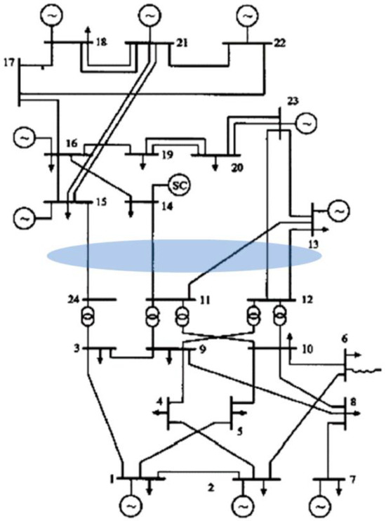
Figure 2.
One-line diagram of the test system, highlighting the interface between voltage levels. The numbers reported in the diagram represent the bus identifiers.
According to the geolocalization assumptions above, the probabilistic model for wet snow events on the test system was elaborated starting from the meteorological reanalysis dataset MERIDA [30] which accounts for past weather events that also occurred in the area under study. In the present case study, the generation of the threat/load/renewable generation scenarios performed using the Copula theory formulation in Section 3.1.2 assumes that there is no correlation between load demand and renewable generation, while there is a negative correlation of −0.8 between the threat intensity and the renewable generation which accounts for potential reductions in the power production from renewable plants due to adverse weather conditions (this also represents a conservative assumption for resilience assessment analyses). The discussion of possible methods to select the representative scenarios is out of the scope of the paper.
The failure return periods of the 33 OHLs of the test system are obtained by combining the abovementioned wet snow probabilistic models with the vulnerability models for the lines. Table 1 reports the failure return periods (RP) for the branches which are assumed to be more frequently affected by the same extreme weather event. This means that the correlations among the events of a simultaneous exceedance of a high value for the threat stress variable (e.g., high linear load of wet snow) at these lines are the highest ones, given the historical recorded events. A correlation matrix R, already introduced in Section 3.1.2, is used to describe the correlation of these exceedance events over the lines of the test system. With reference to the clustering process of the grid assets recalled in Section 3.1.2, the matrix R reported in Table 2 is characterized by a high positive correlation among the first five branches (0.9) and between the last two OHLs (0.8). Thus, the tool considers these two clusters of OHLs with correlated weather events for the generation of the multiple contingencies. The average yearly increases in load and generation capacity are set to 1 and 5%, respectively. The adopted average discount rate over multi-year interval is 4%, as in [31].

Table 1.
Failure return periods for the OHLs with the highest correlations among the events of simultaneous exceedance of a high value for the threat stress variable.
Table 2.
The linear correlation matrix R (b) for the OHLs with the highest correlations among the events of simultaneous exceedance of a high value for the threat stress variable.
Two hardening measures are considered:
- The reinforcement of OHL subcomponents (in particular, towers): in the optimization framework, the model of this countermeasure was applied by moving the vulnerability curve of the OHL subcomponents (specifically towers) towards higher values of the stress variables (wet snow linear mass in kg/m), thus representing a higher resistance of such a subcomponent to wet snow actions.
- The application of antitorsional devices to increase torsional rigidity of the wires (shield wires and conductors), thus preventing the formation of wet snow sleeves: the model of this countermeasure was performed by reducing the wet snow load to which the OHL subcomponents are subject in the “HIGH threat” scenarios described below by a derating factor which depends on the number and spacing of antitorsional devices on the line spans, according to the model the authors introduce in [32].
The preventive measure is the redispatch of conventional generation to avoid cascading tripping due to overloads, while the corrective action consists of load shedding actions performed in the case of contingency occurrence to relieve potential security problems.
The unitary costs adopted for the resilience enhancement measures are adapted from [31] and they are reported in Table 3.
Table 3.
Unitary costs for active and passive measures (amu = arbitrary monetary unit).
Unless differently specified, the cost of emergency load shedding is set equal to the cost of the energy not served, i.e., 4 × 10⁴ amu/MWh.
The optimization cases described in this paper assume realistic values for the upward and downward redispatching costs, which are applied to all generators. However, specific upward and downward redispatching costs can be set for each generating unit. Antenna connections were excluded from the reinforcement candidates because the fulfillment of the security criterion is strictly required; thus, any investment aimed at assuring the security criterion (such as the reinforcement of antenna connections) can be ascribed as a benefit to system security rather than to its resilience.
Both OFs mentioned in Section 3.2 are used in the optimization. The final level of resilience of the system is measured through the residual EENS associated with the scenarios after the deployment of the optimal portfolio of resilience enhancement measures.
Though the methodology is general, its assumed that two discrete states (“HIGH” and “LOW”) are set for load, generation, and threat variables. In particular, Table 4 reports the correspondence between the scenario ID and the value (H or L, standing for “HIGH” or “LOW”, respectively) for each discretized variable. It is worth noting that for any climatological interval, each variable (load, generation, and threat intensity) can assume two values, “Low” and “High”; however, the same sequence is associated with different scenarios because, e.g., the “High” level for the load variable in the first climatological value corresponds to a different load demand with respect to the “High” level for the load variable in the second and the third climatological intervals due to the evolution of load demand among the intervals. A similar consideration applies to the generation variable “G” due to the evolution of renewable installed power over the decades. In addition, the probability associated with the “High” level of threat intensity changes over the climatological intervals due to climate change effects. This explains why different scenarios are associated with the same sequence of “High” and “Low” values of the stochastic inputs of the problem.
Table 4.
Correspondence between scenarios and levels H and L for threat (TH), load (L), and generation (G) variables.
The “initial” operating point for each scenario of load and renewable generation has been computed using an AC OPF which evaluates the most convenient dispatch of conventional generators in order to assure the N security of the initial operating points.
Three intervals (p = 1, …, 3) are considered with a length of 10 years each. The climatic scenarios adopted for the optimization cases refer to the three intervals 2021–2030, 2031–2040, and 2041–2050. They stem from the elaboration of an ensemble of climatological models [26] and are discussed in Section 3.4.2. The elaboration provides the probability of overcoming the critical value of wet snow linear mass (8 kg/m) for any point of a regular mesh in the portion of the area under study and for each of the three 10-year climatological intervals.
The two probabilistic models discussed in Section 3.4.2, MOD1 and MOD2, were adopted for climate evolution. For illustrative purposes, Figure 3a–c shows the maps of the probability of overcoming the 8 kg/m threshold of wet snow linear mass referring to the northeast of Italy for the three climatological intervals and considering the MOD2 model to probabilistically represent the CC effects.
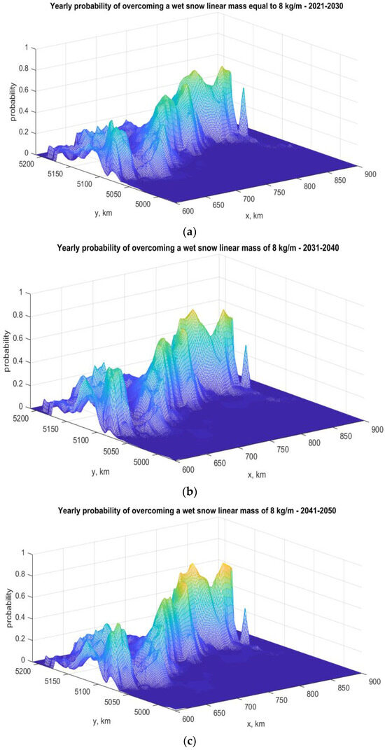
Figure 3.
(a–c) Map of the probability of overcoming the critical wet snow linear mass (8 kg/m) for three different climatological intervals (2021–2030, 2031–2040, and 2041–2050) based on probabilistic model MOD2 for CC effects.
Table 5 summarizes the description and the goal of each described optimization case. For each case, the tool computes the residual EENS, the SUI, and the TNB indexes, in addition to all the costs related to the active and passive measures.
Table 5.
Summary of the optimization cases on IEEE RTS.
The assessment of power system resilience, considering the MOD1 model for climate change effects and no resilience enhancement measures deployed over the 30-year horizon, starts from the selection of the N-k contingencies for each scenario on the basis of the screening methodology described in Section 3.1.2. The performed resilience assessment analysis shows the following:
- In the most stressed operating points (scenario #6), 27 N-k contingencies with not-negligible probability are detected, of which 6 (listed in Table 6) are critical because they provoke significant amounts of energy not served mainly due to cascading failures along the interface between the 230 and 138 kV areas. The blue area in Figure 2a includes the lines affected by the threat. Each line in Table 6 is represented as “Bx-By”, where “x” and “y” are the IDs of the buses corresponding to the line terminals.
Table 6. List of contingencies causing energy not served in stressed scenario #6.Table 6. List of contingencies causing energy not served in stressed scenario #6.
Contingency ID Contingency Description ENS (MWh) 1 B11-B13; B11-B14; B12-B13; B15-B24 2.1418 × 10⁴ 2 B11-B13; B11-B14; B12-B13; B12-B23 4.5828 × 10⁴ 3 B11-B14; B12-B13; B12-B23; B15-B24 2.1418 × 10⁴ 4 B11-B13; B12-B13; B12-B23; B15-B24 2.4538 × 10⁴ 5 B11-B13; B11-B14; B12-B23; B15-B24 2.1418 × 10⁴ 6 B11-B13; B11-B14; B12-B13; B12-B23; B15-B24 2.1418 × 10⁴ More specifically, the critical contingencies consist of N-4 and N-5 contingencies on the branches of the interface between the 138 and 230 kV areas of the grid. Contingencies #1, 3, and 5 cause the overload of the remaining line connecting the two areas with its consequent tripping and the separation of the two areas. This in turn causes the loss of all the load nodes in the 138 kV area due to a generation deficit.Contingency #2 causes the overloading of branches B24-B15, B24-B03, and B03-B09: the largest overload affects branch B03-B09, which trips first. This causes in turn an unsustainable operating point (indicated by the load flow divergence in the post-tripping condition): this is quantified by assuming the complete blackout of the RTS grid.Contingency #6 directly causes the separation of the 230 and 138 kV areas of the grid, with the consequent blackout of the 138 kV area due to a generation deficit.In other scenarios with a “HIGH” load associated with climatological intervals 2 and 3 (e.g., scenarios 14 and 22 in Table 4), similar cascade patterns as the ones in scenario 6 are identified. - The total EENS is equal to 2.075 × 10³ MWh over 30 years under the MOD1 hypothesis, mainly due to the contingencies triggering the cascade patterns above in the three climatological intervals. As reported in Section 4.4.1, adopting MOD2 for CC effects leads to a different (in particular, a higher) value of the total EENS.
The typical output of the optimization cases consists of the optimal portfolio of measures to boost resilience, obtained by maximizing one of the two OF alternatives, i.e., the Total Net Benefit (TNB) or the System Utility Index (SUI) introduced in Section 2.3. The costs of the measures are summed up in a table for each optimization case:
- The actual costs for hardening solutions (tower support hardening or antitorsional device installation and maintenance);
- The expected costs for preventive and corrective measures deployed. The term “expected” is used to clarify that the costs also include the probability of occurrence of extreme events and the probability of N-k contingencies (the latter is included in the costs for corrective measures).
4.1. Base Case with Model MOD1 for CC Effects (Sim 1)
Table 7 and Table 8 report the portfolio of resilience enhancement measures suggested by the methodology based on the unitary costs in Table 3. The meaning of the scenario IDs reported in brackets in the rows related to active measures in result tables such as Table 7 is explained in Table 4, while the lines which undergo a hardening measure are represented by the codes of their terminal nodes (“Bxx”) separated by a dash.
Table 7.
Portfolio of active and passive measures suggested with TNB-based OF. Optimization case sim 1, model MOD1 for CC effects.
Table 8.
Portfolio of active and passive measures suggested by SUI-based OF. Optimization case sim 1, model MOD1 for CC effects.
It is worth noting that for both OFs hardening solutions are identified. In the TNB-oriented optimization, the relatively low costs for antitorsional devices favor the adoption of such a measure from the first interval. The residual EENS passes from 2.075 × 10³ MWh in the base case to 0 MWh; the TNB is equal to 5.6585 × 10⁷ amu over 30 years and the SUI is equal to 93.89. In the SUI-based optimization, the TNB is equal to 1.0464 × 10⁷ amu (lower than the one obtained with TNB optimization) and the SUI is 139.52 (larger than the one in the TNB-oriented optimization): the residual EENS in the case of the SUI-based optimization for the wet snow threat is 1702 MWh. The passive measure consists of the deployment of antitorsional devices on branches B12-B13 and B11-B14 in intervals 1 and 3, respectively, in the TNB-based optimization, while in the SUI-based optimization antitorsional devices are applied only to branch B11-B14 in interval 1. The corrective actions, which consist of load- and generation-shedding actions, are deployed in the stressed scenarios in intervals 1 and 2 only in the TNB-based optimization. It is worth noting that for any passive measure the optimization methodology accounts for the relevant capital costs in the first interval (e.g., interval 1 for the deployment of anti-torsional devices in branch B12-B13) and the relevant operational costs (much smaller than the capital ones) in the subsequent intervals (e.g., intervals 2 and 3 for branch B12-B13 in Table 7).
4.2. Effect of the Increase in the Unitary Capital Cost of the Antitorsional Devices in the Case of Model MOD1 for CC Effects (Optimization Case 2)
From the base case, it is evident that the most cost-effective hardening solution is the application of antitorsional devices instead of support/line hardening measures (as expected). The second case considers a higher unitary cost for the application of the antitorsional devices (from 100 to 250 amu/device). The optimized portfolios of resilience enhancement measures are reported in Table 9 for the TNB-based optimization.
Table 9.
Portfolio of active and passive measures suggested with TNB based OF. Optimization case 2, model MOD1 for CC effects.
In this case, the total SUI (TNB) over 30 years is equal to 43.02 (5.5864 × 10⁷ amu): in particular, the results show a slight decrease in the TNB with respect to the base case (from 5.6585 × 10⁷ amu to 5.5864 × 10⁷ amu) due to the higher capital costs for antitorsional devices. However, the portfolio is less cost-effective with respect to the one proposed in the base case; in fact, the SUI index passes from 93.89 to 43.02. In the SUI-based optimization (see Table 10), the SUI (TNB) over 30 years passes from 139.52 (1.0464 × 10⁷ amu) to 66.26 (2.0506 × 10⁵ amu). It is worth noting that the TNB drastically decreases because no passive measures are suggested because of the higher capital costs in this optimization case: the only active measure deployed is a corrective action in interval 3, which results in a limited TNB over the 30-year horizon. The residual EENS is very high (2055 MWh), with only a 1% reduction in its initial value.
Table 10.
Portfolio of active and passive measures suggested with SUI based OF. Optimization case 2, model MOD1 for CC effects.
4.3. Effect of Lower Unitary Costs for the Deployment of Corrective Actions in the Case of Model MOD1 for CC Effects (Optimization Case 3)
This case assumes the same values of costs as in optimization case 2, but the unitary costs for the corrective actions are lowered from 4 × 10⁴ to 4 × 10³ amu/MWh. The optimal portfolios of resilience enhancement measures are reported in Table 11 and Table 12 respectively for the TNB- and SUI-oriented optimizations. In the TNB-based optimization, the SUI (TNB) index increases from 43.02 (5.5864 × 10⁷ amu) to 58.18 (5.6210 × 10⁷ amu) thanks to the reduction in the unitary costs of corrective actions. For the same reason, in the SUI-based optimization, the SUI (TNB) index increases from 66.27 (2.0507 × 10⁵ amu) to 648.13 (2.0789 × 10⁵ amu).
Table 11.
Portfolio of active and passive measures suggested with TNB-based OF. Optimization case 3, model MOD1 for CC effects.
Table 12.
Portfolio of active and passive measures suggested with SUI based OF. Optimization case 3, model MOD1 for CC effects.
In the SUI-based optimization, the choice to deploy the corrective action measures only in interval 3 is linked to the need to maximize the SUI index over 30 years: assuming the SUI as the OF implies the selection of the most cost-effective measure, and thus also a not-negligible residual EENS (equal to 2.055 × 10³ MWh over 30 years for this optimization case).
If one poses a constraint to the maximum admissible residual EENS (e.g., set to 1000 MWh), the SUI-based optimization indicates a different portfolio (see Table 13), where the corrective actions are deployed in all three climatological intervals: the residual EENS is 631.86 MWh, but the SUI is lower than in the previous case (388.48 versus 648.13). However, the TNB for this case is equal to 3.3518 × 10⁷ amu (higher than the 2.0789 × 10⁵ amu obtained from the SUI-based optimization without the minimum residual EENS constraint, but lower than 5.5864 × 10⁷ amu, the TNB obtained from the TNB-based optimization).
Table 13.
Portfolio of active and passive measures suggested with SUI and a constraint on maximum admissible residual EENS (set to 103 MWh). Optimization case 3, model MOD1 for CC effects.
4.4. Effect of the Probabilistic Model for CC Effects (Optimization Case 4)
The same optimization cases previously described (simulations 1, 2, and 3) were re-run utilizing the model MOD2. First of all, the initial “performance” of the system in terms of EENS with no measures deployed is different due to the different estimation of the frequency of extreme events with the new probabilistic modeling for CC effects. In particular, the initial EENS is about 4.5435 × 10³ MWh, against the 2.075 × 10³ MWh evaluated with the previous model: this is due to the fact that the current modeling assumes that extreme events show higher probabilities of occurrence in each climatological interval as well as larger increases in their probabilities between subsequent intervals, with respect to the MOD1 model for CC effects.
4.4.1. Base Case (Optimization Case 4a)
This case assumes the unitary cost for the corrective action and the capital cost for antitorsional devices shown in Table 3. The portfolio suggested by the TNB-based and SUI-based optimizations are reported respectively in Table 14 and Table 15.
Table 14.
Portfolio of active and passive measures suggested with TNB-based OF. Optimization case 4a, model MOD2 for CC effects.
Table 15.
Portfolio of active and passive measures suggested with SUI-based OF. Optimization case 4a, model MOD2 for CC effects.
With model MOD2, the SUI-based optimization suggests the deployment of antitorsional devices in the third climatological interval: the high probability of occurrence of extreme events, which characterizes the MOD2 mode, together with the relatively high unitary costs of active measures (40 kamu/MWh for corrective actions), makes less convenient the deployment of active measures, which are activated only in the case of adverse weather (preventive actions) and/or of contingency occurrence (corrective actions).
The residual EENS is equal to 3.1584 × 10³ MWh (due to the absence of the measure in intervals 2 and 3) and the SUI (TNB) is equal to 199.07 (3.3981 × 10⁷ amu). The TNB-based optimization results in a negligible residual EENS: the SUI (TNB) is equal to 133.87 (1.1810 × 10⁸ amu). It is worth noting that the different probabilistic model for the climate evolution determines different probabilities of occurrence of the N-k contingencies associated with the not-null ENS, which in turn determines different prioritizations of the line interventions (specifically, the deployment of antitorsional devices).
In particular, the model MOD1 for CC effects applied to the TNB-based optimization suggests the deployment of such devices on lines B12-B13 and B11-B14, while the model MOD2 for CC effects indicates the convenience to deploy such devices on branches B11-B13 and still B11-B14. The selection of branch B11-B13 in the SUI-based optimization is due to the fact that this branch is the most cost-effective compromise between capital/operational costs and the benefit to resilience obtained from the upgrade of the branch.
The introduction of the maximum admissible residual EENS constraint in the SUI-based optimization results in a less cost-effective solution: Table 16 reports details about the portfolio suggested by the algorithm.
Table 16.
Portfolio of active and passive measures suggested through SUI-based optimization with residual EENS constraint. Optimization case 4a, model MOD2 for CC effects.
The SUI index decreases from 199.07 to 144.35 (which is however higher than the SUI index obtained from the TNB-based optimization). This constraint allows a higher TNB value (from 3.3981 × 10⁷ amu to 9.2016 × 10⁷ amu). The deployment of antitorsional devices on branch B11-B13 is anticipated from interval 3 to interval 1, and this type of measure is applied also to branch B11-B14 in interval 3. The residual EENS is equal to 996 MWh.
4.4.2. Higher Capital Costs for the Antitorsional Devices (Sim 4b)
This scenario assumes a higher capital cost for antitorsional devices (from 100 to 250 amu/device) in the presence of the model MOD2 for CC effects. No significant changes are found in the solutions with respect to sim 4a (see Table 17 and Table 18): in the TNB-based optimization, in particular, the increase in the antitorsional capital costs reduces the TNB (from 1.1810 × 10⁸ to 1.1625 × 10⁸ amu) and the SUI index (from 133.86 to 43.48).
Table 17.
Portfolio of active and passive measures suggested with TNB-based OF. Optimization case 4b, model MOD2 for CC effects.
Table 18.
Portfolio of active and passive measures suggested with SUI-based OF. Optimization case 4b, model MOD2 for CC effects.
In particular, the solution suggested changes from a mix of active and passive measures (sim 4a) to the deployment of only passive measures to three branches (B11-B13, B11-B14, and B12-B13) instead of two (B11-B13, B11-B14). This counterintuitive solution is due to the fact that the additional benefit obtained from the deployment of antitorsional devices on branch B12-B13 in interval 3 and the anticipation of the deployment of the same device type on branch B11-B14 from interval 3 to interval 1 plus the reduction in the costs for active measures in the three intervals overcome the additional costs due to the increase in the (both capital and operational) costs related to the passive measures.
The SUI-based optimization suggests also deploying corrective actions in the three intervals to compensate for the higher costs of passive measures to be deployed in the third interval: the SUI index decreases from 199 to 43.49. However, the TNB over 30 years passes from 3.3981 × 10⁷ amu to 6.4147 × 10⁷ amu, thanks to the lower ENS in the first two intervals. The residual EENS improves from 3.1584 × 10³ MWh (in sim 4a) to 2044 MWh.
Again, the introduction of the maximum admissible residual EENS constraint into the SUI-based optimization brings a lower SUI index (passing from 84.63 to 64.48) but a higher TNB value (from 6.4147 × 10⁷ amu to 9.6368 × 10⁷ amu). The residual EENS is equal to 800 MWh, thus lower than 1000 MWh (the maximum value set for the optimization case). Table 19 reports details about the portfolio suggested by the algorithm.
Table 19.
Portfolio of active and passive measures suggested through SUI-based optimization with residual EENS constraint. Optimization case 4b, model MOD2 for CC effects.
4.4.3. Lower Unitary Costs for the Corrective Actions (Sim 4c)
Starting from the unitary costs of 250 amu/device set in optimization case 2, this case assumes a lower unitary cost for corrective actions (from 4 × 10⁴ to 4 × 10³ amu/MWh) in the presence of model MOD2. The results of the TNB-based optimization do not change with respect to the outputs of optimization case 4b.
Table 20 reports the portfolios of measures proposed using the SUI-based OF: the optimizer suggests a portfolio of corrective action measures still applied in interval 1, and the deployment of such measures in intervals 2 and 3 would also bring lower SUI indexes. The residual EENS is equal to 4.2707 × 10³ (−6% with respect to the base case), while the SUI (TNB) index is equal to 1090.91 (2.6119 × 10⁶ amu). In addition, for this case, the constraint of the maximum residual EENS is applied to the SUI-based optimization.
Table 20.
Portfolio of active and passive measures suggested with SUI-based OF without residual EENS constraint. Optimization case 4c, model MOD2 for CC effects.
Table 21 reports the relevant results considering a maximum residual EENS equal to 1000 MWh. The residual EENS is equal to 800.33 MWh, which is lower than the constraint; however, the SUI is 181.18, which is lower than the SUI value (1090.91) previously obtained without any constraint on the residual EENS. This means that the cost effectiveness of the measure decreases if a minimum residual EENS target is also set: in fact, in order to reach the residual EENS target, only active measures are not sufficient, and the methodology suggests deploying a passive measure (applying the antitorsional devices) on branch B11-B13 in interval 3. The relatively higher costs for passive measures—with respect to active measure costs—cause a reduction in the cost effectiveness of the portfolio.
Table 21.
Portfolio of active and passive measures suggested through SUI-based OF with residual EENS constraint of 1000 MWh. Optimization case 4c, model MOD2 for CC effects.
As far as the time performance of the solution algorithm is concerned, the mean computation time over all the optimization cases is around 15 min on an Intel® Xeon® Gold 6248R CPU, 128 GB RAM, two-processor 3.00 GHz machine. The maximum number of iterations run by the two-stage algorithm over all the optimization cases is 3 (significantly lower than the maximum number of iterations set to 20).
5. Application to a Real-World Case Study
This section presents and discusses the application of the methodology to a realistic system to demonstrate its scalability to large systems.
5.1. Test System and Optimization Cases
The test system is a model of a significant portion of the Italian transmission and sub-transmission system dated back to the early 2000s and located in the northeast of the peninsula: it is worth noting that the adopted grid and its operating points are used only for research purposes, and they do not reflect the way the TSO currently manages the same grid portion. The adopted model contains 700 electric nodes, about 800 lines (cables and OHLs), and 100 generators. The load demand was increased by 10% with respect to the available operating point to stress the system. In the present case study, the generation of the threat/load/renewable generation scenarios is still performed using the Copula theory formulation in Section 3.1.2, and it considers the same linear correlation coefficients among the three variables Th, L, and G reported in Section 4. The “high” and “low” values of the variables “load” and “renewable generation” for future climatological intervals are derived from the available statistics (e.g., duration curves) and from the rates of increase in load demand and installed renewable generation.
Figure 4a,b reports the one-line diagrams of the two grid areas where the grid interventions suggested by the methodology are located. For confidentiality reasons, all the substation names were anonymized.
Figure 4.
One-line diagram of the two areas under study in the 132 kV Italian grid in the Dolomites (a) and in the South-Eastern Alps (b), with an explicit indication of the bus code only for the grid nodes mentioned in the results subsection. Arrows, dots, lines and circles with “G” symbol represent respectively loads, buses, branches and generators.
The threat under study is wet snow, which is a major cause of failures in the region under study. The set of active and passive measures, the unitary costs of the measures (Table 3), and the probabilistic models MOD1 and MOD2 for CC effects are the same as the ones used in the previous case study and described in Section 3.4.2.
Again, both the OFs mentioned in Section 3.2 are used in the optimization. The final level of resilience of the system is measured through the residual EENS associated with the scenarios after the deployment of the optimal portfolio of resilience enhancement measures.
Table 22 summarizes the description and the goal of each described optimization case. For each case, the tool computes the residual EENS and the SUI and TNB indexes, in addition to all the costs related to the active and passive measures.
Table 22.
Summary of the optimization cases for the real world case study.
Unlike the cases on the IEEE RTS, the optimization cases on the realistic power system model were run considering a maximum order of contingency (number of simultaneously failed components) equal to 5 and a maximum number of candidates for passive measures equal to 30. Under these assumptions, the computation time is around 45 min for each optimization case using an Intel® Xeon® Gold 6248R CPU, 128 GB RAM, two-processor 3.00 GHz machine. The increase in the contingency set cardinality as well as of the number of candidates for passive measures result in higher computational times.
5.2. Optimization Case 1: The Base Case
Table 23 reports the costs for active and passive measures in the case of the TNB-based optimization: it is worth noticing that antitorsional devices (much cheaper than tower support reinforcements) are selected to harden lines BUS1-BUS2 and BUS5-BUS2 in the Alpine area of Cencenighe and lines BUS3-BUS4 in the Cadore area (see Figure 5a) since the first climatological interval, while the hardening of line BUS3-BUS6 is postponed to the third climatological interval. This allows a reduction in the EENS indicator from 228.7 MWh to 38.5 MWh over the 30-year horizon. The final SUI index is equal to 33.6 over the 30-year horizon, and the Total Net Benefit is equal to 6.9 × 10⁶.
Table 23.
Optimal portfolio suggested with TNB based OF. Model MOD1 for CC effects.
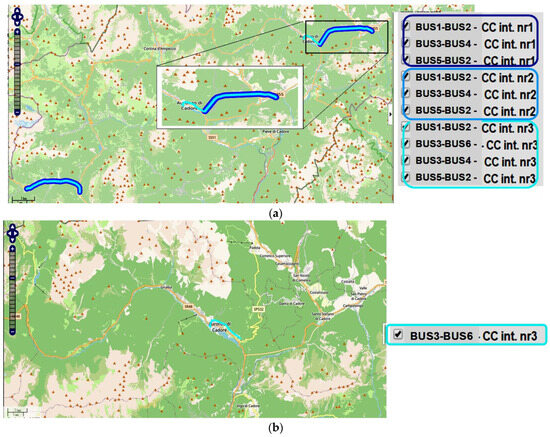
Figure 5.
Location of the line to be hardened according to the TNB-based (a) and SUI-based (b) optimizations in the case of MOD1 model for CC effects and standard unitary costs as from Table 3. Dark blue, blue, and cyan lines indicate the lines which undergo the deployment of antitorsional devices in climatological intervals 1, 2, and 3, respectively.
Table 24 reports the portfolio of resilience enhancement measures suggested by the methodology in the case of an SUI-centered optimization: it is worth noting that only the hardening intervention on branch BUS3-BUS6 is suggested in the third climatological interval (see Figure 5b). In fact, the SUI index suggests more cost-effective solutions (as it optimizes the ratio and not the difference between benefits and costs). Even though lower expenses are required with the SUI-based indicator, the residual EENS obtained from this SUI optimization is much higher than under the TNB-based optimization (183 MWh, a 20% reduction in the initial EENS, against 38.5 MWh, which represents an 84% reduction in the same initial EENS). The TNB and SUI attained with the SUI-driven optimization are equal to 2.0493 × 10⁶ amu and 116.45, respectively.
Table 24.
Optimal portfolio suggested with SUI based OF. Model MOD1 for CC effects.
It is worth noting that no active measures are suggested, because the proposed active measures are aimed at stopping potential cascading failures (by correctively shedding loads or preventively redispatching generators); however, in the grid portion under study, most of the contingencies with the highest probabilities do not imply cascading failures but simply consist of the damages to the lines feeding the primary substations causing the lack of supply to customers. This point represents an interesting outcome of the analysis because the methodology highlights the application limits of operational measures in enhancing power system resilience.
5.3. Optimization Case 2: Effect of a Different Probabilistic Model for CC Effects
The base case scenario was re-run starting from the probabilistic model MOD2 for climate evolution, which assumes a more significant change in the climate over the intervals.
Table 25 and Table 26 indicate the solution for the two optimization runs respectively with TNB and SUI based OF’s: in particular, it is worth noting that the TNB-driven optimization suggests a more expensive mix which, however, is more effective in reducing the residual EENS in the system (passing from 436 MWh before the optimization to 34.2 MWh after the optimization). The envisaged solution consists of applying the antitorsional devices to lines BUS3-BUS6 and BUS3-BUS4 in the Cadore area already in the first climatological interval and postponing the application of antitorsional devices to line BUS7-BUS8 in the Tolmezzo area to the third climatological interval. The TNB attained is equal to 2.1077 × 10⁷ amu, while the SUI is 87 (around 3 SUI points per year).
Table 25.
Optimal portfolio suggested with TNB based OF. Model MOD2 for CC effects.
Table 26.
Optimal portfolio suggested with SUI based OF. Model MOD2 for CC effects.
The SUI-driven optimization favors more cost-effective solutions at the expense of the residual EENS, which is higher (335 MWh wrt 34.2 MWh). The relatively high probability of extreme events suggests the adoption of an economic passive measure, i.e., the antitorsional devices, to lines BUS3-BUS9 and BUS3-BUS6 in the third climatological interval. In fact, though the TNB is lower than in the TNB-driven optimization (6.5061 × 10⁶ versus 2.1077 × 10⁷), the SUI is higher (142.4 versus 87 from the TNB-based optimization).
With respect to the probabilistic model MOD1 in sim 1, some interventions are common to optimization cases 1 and 2 (e.g., the anti-rotational devices are installed on lines BUS3-BUS6 in both optimization cases); however, the more significant changes in the climate evolution in sim 2 also suggest the need to reinforce another line, BUS7-BUS8, with anti-rotational devices in a lower-altitude area (Tolmezzo area, see Figure 6), where according to model MOD2 heavier wet snow events have a higher probability of occurring in the third climatological interval. The higher probabilities of extreme events associated with model MOD2 explain the higher SUI values and TNB values achieved in sim 2 with respect to sim 1.
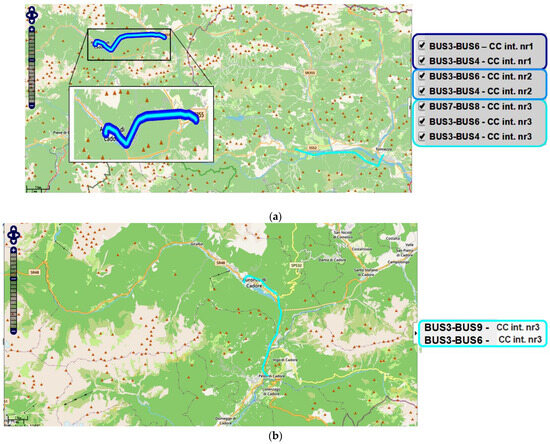
Figure 6.
Location of the line to be hardened according to the TNB-based (a) and SUI-based (b) optimization in the case of MOD2 model for CC effects and standard unitary costs as from Table 3. Dark blue, blue, and cyan lines indicate the lines which undergo the deployment of antitorsional devices in climatological intervals 1, 2, and 3, respectively.
6. Conclusions
The paper presented an Optimization via Simulation and scenario-based methodology aimed at finding the optimal mix of active and passive measures to boost system resilience to natural threats, also accounting for climate change effects and potential cascading failures. The proposed framework can be applied to any threat and any measure, it is very flexible, and it allows an efficient simulation of large portions of realistic power systems, which makes it adequate for TSO decision making for the prioritization of the interventions in the grid.
The application to the test system highlighted the ability of the methodology to indicate lines for passive measure deployment according to the optimization target, which can be chosen between Total Net Benefit (TNB) and System Utility Indicator (SUI) maximization. Moreover, the application has proven the sensitivity of the resulting mix of measures with respect to their unitary costs and to the climate change effects.
The case study applied to a large portion of the Italian transmission system subject to a wet snow threat demonstrates the applicability of the methodology to realistic-scale problems. As a general consideration, the TNB-based optimization and the SUI-based optimization with a constraint on the maximum admissible residual EENS appear to provide the most promising tradeoffs between technical effectiveness and cost efficiency.
Future works will consist of extending the optimization framework to other natural threats of interest (such as wind and floods) and of enlarging the library of available models for resilience enhancement measures.
Author Contributions
Conceptualization, E.C. and D.C.; methodology, E.C. and A.P.; software, A.P.; validation, E.C.; writing—original draft preparation, A.P.; writing—review and editing, E.C. and D.C.; supervision, E.C. All authors have read and agreed to the published version of the manuscript.
Funding
This work has been financed by the Research Fund for the Italian Electrical System under the Three-Year Research Plan 2022–2024 (DM MITE n. 337, 15.09.2022) in compliance with the Decree of 16 April 2018.
Data Availability Statement
Data on the Italian grid is unavailable due to confidentiality restrictions.
Conflicts of Interest
The authors declare no conflict of interest.
Nomenclature
| Cost–Benefit Analysis formulation | |
| set of corrective measures deployed for j-th contingency at hour h | |
| specific hardening configuration | |
| set of preventive measures deployed at hour h | |
| Xh | system state at hour h before the application of preventive measures |
| Xh′ | system state at hour h after the application of preventive measures |
| economic benefit for deploying corrective and pre-ventive actions on system state at hour h potentially subject to topo-logical hardenings of set | |
| costs for deploying corrective and preventive actions on system state at hour h potentially subject to topo-logical hardenings of set | |
| TNB | Total Net Benefit |
| SUI | System Utility Index |
| Scenario-based formulation of the optimization problem | |
| Np | number of climatological intervals |
| NL | number of load scenarios per climatological interval |
| NG | number of generation scenarios per climatological interval |
| NL,G = NL × NG | number of load/generation scenarios characterizing the system operating conditions per climatological interval |
| Nth | number of threat scenarios per climatological interval |
| N | Np × NL,G × Nth, total number of scenarios |
| n = 1, …, N | generic scenario (i.e., combination of climatological interval, load/generation scenario, and threat scenario) |
| p = 1, …, Np | generic climatic interval |
| Critical contingency | contingency causing ENS > 0, where ENS is the energy not served |
| Cn | set of the critical contingencies for scenario n |
| λn | set of lines involved in Cn, i.e., union of the lines of Cn |
| Λ | set of lines involved in Cn over all the N scenarios, i.e., union of λn over all the N scenarios |
| En | set of ENS of Cn in the initial configuration with “no measures” |
| NPL | number of available types of passive measures |
| conditional probability of occurrence of operating condition st associated with climatological interval p, given a certain threat value Th | |
| vector of binary decision variables with length NPL × Ncomp × Np for the deployment of the NPL passive measures on Ncomp components in the Np climatological intervals | |
| vector of binary decision variables with length N related to the deployment of preventive measures aimed to improve security of current scenario n corresponding to system operating condition st in the p-th climatological interval and for threat intensity value th | |
| vector of binary decision variables with length N related to the deployment of a corrective measure aimed at limiting the impact of contingencies which can occur in the current scenario n corresponding to system operating condition st (possibly modified by preventive measures) in the p-th climatological interval and for threat intensity value th. | |
| maximum admissible costs for the deployment of preventive measures | |
| maximum admissible costs for the deployment of corrective measures | |
| maximum admissible costs for the deployment of passive measures | |
| Threat and climate change modeling | |
| RPi | outage return period for i-th branch |
| probability of exceeding critical load over the spans of branch i derived from reanalysis of past events | |
| probability of exceeding critical load over the spans of branch i from climate change modeling for p-th climatological interval. | |
| Two-stage solution algorithm | |
| ℑ | set of candidate lines for reinforcements at the beginning of Stage 1 in the optimization algorithm |
| Λl | set of climatological intervals in which line l ∈ ℑ is a candidate for reinforcements |
| Nd | number of sequences of the deployment of passive measures on the candidate lines over the climatological intervals, |
| vector of binary decision variables representing the solution at the end of Stage 1 and iteration q | |
| OF variation at first checkpoint at iteration q where OF is the objective function | |
| OF variation at second checkpoint at iteration q | |
| XCP | subvector of generic solution X, including the binary decision variables which indicate the potential activation of preventive and corrective action measures in the N scenarios, thus dim(XCP) = 2 × N |
| ϒ(q) | subset of lines of set ℑ which are selected by the proposed algorithm at Stage 1 at iteration q of the optimization and remain candidates in Stage 2 |
| vector of binary decision variables representing the solution at the end of Stage 2 and iteration q, ) = dim(ϒ(q)) + 2 × dim(XCP) | |
| vector of binary decision variables representing a guess solution at the end of Stage 2 and iteration q | |
References
- Papic, M.; Ekisheva, S.; Robinson, J.; Cummings, B. Multiple outage challenges to transmission grid resilience. In Proceedings of the 2019 IEEE Power Energy Society General Meeting (PESGM), Atlanta, GA, USA, 4–8 August 2019; pp. 1–5. [Google Scholar]
- CIGRE WG C4.47. Defining power system resilience. Electra CIGRE J. 2019, 316, 1–3. [Google Scholar]
- ACER (EU Agency for the Cooperation of Energy Regulators). Opinion of ACER on ENTSO-e 3rd Draft Guideline for Cost Benefit Analysis of Grid Development Projects; ACER: Ljubljana, Slovenia, 2020; pp. 1–31. [Google Scholar]
- Panteli, M.; Trakas, D.N.; Mancarella, P.; Hatziargyriou, N.D. Power Systems Resilience Assessment: Hardening and Smart Operational Enhancement Strategies. Proc. IEEE 2017, 105, 1202–1213. [Google Scholar] [CrossRef]
- Ciapessoni, E.; Pitto, A.; Cirio, D. An Application of a Risk-Based Methodology to Anticipate Critical Situations Due to Extreme Weather Events in Transmission and Distribution Grids. Energies 2021, 14, 4742. [Google Scholar] [CrossRef]
- Moreno, R.; Strbac, G. Integrating high impact low probability events in smart distribution network security standards through CVAR optimisation. In Proceedings of the IET International Conference on Resilience of Transmission and Distribution Networks (RTDN), Birmingham, UK, 22–24 September 2015; pp. 1–6. [Google Scholar]
- Lagos, T.; Moreno, R.; Espinosa, A.N.; Panteli, M.; Sacaan, R.; Ordonez, F.; Rudnick, H.; Mancarella, P. Identifying Optimal Portfolios of Resilient Network Investments Against Natural Hazards, With Applications to Earthquakes. IEEE Trans. Power Syst. 2019, 35, 1411–1421. [Google Scholar] [CrossRef]
- Cesena, E.A.M.; Zhou, Y.; Gutierrez, J.N.M.; Zhu, W.; Panteli, M.; Mutale, J.; Mancarella, P.; Tomlinson, J.; Baisie, R.; Obuobie, E.; et al. Quantifying the Impacts of Modelling Assumptions on Accuracy and Computational Efficiency for Integrated Water-Energy System Simulations Under Uncertain Climate. IEEE Trans. Sustain. Energy 2022, 13, 1370–1382. [Google Scholar] [CrossRef]
- Anderson, K.; Li, X.; Dalvi, S.; Ericson, S.; Barrows, C.; Murphy, C.; Hotchkiss, E. Integrating the Value of Electricity Resilience in Energy Planning and Operations Decisions. IEEE Syst. J. 2020, 15, 204–214. [Google Scholar] [CrossRef]
- Zou, B.; Wang, C.; Zhou, Y.; Wang, J.; Chen, C.; Wen, F. Resilient co-expansion planning between gas and electric distribution networks against natural disasters. IET Gener. Transm. Distrib. 2020, 14, 3561–3570. [Google Scholar] [CrossRef]
- Ranjbar, H.; Hosseini, S.H.; Zareipour, H. Resiliency-oriented planning of transmission systems and distributed energy resources. IEEE Trans. Power Syst. 2021, 36, 4114–4125. [Google Scholar] [CrossRef]
- Souto, L.; Yip, J.; Wu, W.Y.; Austgen, B.; Kutanoglu, E.; Hasenbein, J.; Santoso, S. Power system resilience to floods: Modeling, impact assessment, and mid-term mitigation strategies. Int. J. Electr. Power Energy Syst. 2022, 135, 107545. [Google Scholar] [CrossRef]
- Ciapessoni, E.; Cirio, D.; Pitto, A. Cascadings in large power systems: Benchmarking static vs. time domain simulation. In Proceedings of the 2014 IEEE PES General Meeting Conference Exposition, Washington, DC, USA, 27–31 July 2014; pp. 1–5. [Google Scholar]
- Noebels, M.; Preece, R.; Panteli, M. AC Cascading Failure Model for Resilience Analysis in Power Networks. IEEE Syst. J. 2020, 16, 374–385. [Google Scholar] [CrossRef]
- European Commission. Guide to Cost-Benefit Analysis of Investment Projects: Economic Appraisal Tool for Cohesion Policy 2014–2020. 2014. Available online: https://ec.europa.eu/regional_policy/en/information/publications/guides/2014/guide-to-cost-benefit-analysis-of-investment-projects-for-cohesion-policy-2014-2020 (accessed on 18 May 2022).
- ENTSO-E. 4th Guideline for Cost Benefit Analysis of Grid Development Projects. Draft Version 4.0 for Public Consultation. 2022. Available online: https://eepublicdownloads.blob.core.windows.net/public-cdn-container/tyndp-documents/CBA/CBA4/221215_CBA4-Guideline_v1.0_for-public-consultation.pdf (accessed on 23 February 2023).
- Moreno, R.; Panteli, M.; Mancarella, P.; Rudnick, H.; Lagos, T.; Navarro, A.; Ordonez, F.; Araneda, J.C. From Reliability to Resilience: Planning the Grid Against the Extremes. IEEE Power Energy Mag. 2020, 18, 41–53. [Google Scholar] [CrossRef]
- Ciapessoni, E.; Pitto, D.C.A.; Faggian, P.; Pirovano, G.; Marzullo, F.; Falorni, F.; Scavo, F. A Methodology for Resilience-oriented Planning in the Italian Transmission System. In Proceedings of the 2021 AEIT International Annual Conference (AEIT), Torino, Italy, 4–8 October 2021; pp. 1–6. [Google Scholar]
- Heitsch, H.; Römisch, W. Scenario Reduction Algorithms in Stochastic Programming. Comput. Optim. Appl. 2003, 24, 187–206. [Google Scholar] [CrossRef]
- Bompard, E.; Pons, E.; Wu, D. Extended Topological Metrics for the Analysis of Power Grid Vulnerability. IEEE Syst. J. 2012, 6, 481–487. [Google Scholar] [CrossRef]
- Cotilla-Sanchez, E.; Hines, P.D.H.; Barrows, C.; Blumsack, S. Comparing the Topological and Electrical Structure of the North American Electric Power Infrastructure. IEEE Syst. J. 2012, 6, 616–626. [Google Scholar] [CrossRef]
- ENTSO-e. Cost Benefit Analysis for Electricity Balancing—General Methodology. Final Report Prepared by Frontier Economics and Consentec. 2015, pp. 1–34. Available online: https://consultations.entsoe.eu/markets/eb-cba/supporting_documents/150223_NCEB_General_CBA_methodology_for_consultation.pdf (accessed on 18 May 2022).
- Nelsen, R.B. An Introduction to Copulas, 3rd ed.; Springer: New York, NY, USA, 2006. [Google Scholar]
- Carrington, N.K.; Dobson, I.; Wang, Z. Extracting Resilience Metrics From Distribution Utility Data Using Outage and Restore Process Statistics. IEEE Trans. Power Syst. 2021, 36, 5814–5823. [Google Scholar] [CrossRef]
- Ciapessoni, E.; Cirio, D.; Pirovano, G.; Pitto, A.; Marzullo, F.; Lazzarini, A.; Scavo, F. Modeling the overhead line vulnerability to combined wind and snow loads for resilience assessment studies. In Proceedings of the 2021 IEEE Madrid PowerTech, Madrid, Spain, 28 June–2 July 2021; pp. 1–6. [Google Scholar]
- Faggian, P.; Decimi, G. An updated investigation about climate-change hazards that might impact electric infrastructures. In Proceedings of the of 2019 AEIT International Annual Conference (AEIT), Florence, Italy, 18–20 September 2019; pp. 1–5. [Google Scholar]
- Gendreau, M.; Potvin, J.Y. Handbook of Metaheuristics, 2nd ed.; Springer: New York, NY, USA, 2012. [Google Scholar]
- Lewis, R.M.; Torczon, V.; Trosset, M.W. Direct search methods: Then and now. J. Comput. Appl. Math. 2000, 124, 191–207. [Google Scholar] [CrossRef]
- Subcommittee, P.M. IEEE reliability test system. IEEE Trans. Power Appar. Syst. 1979, 98, 2047–2054. [Google Scholar] [CrossRef]
- Bonanno, R.; Lacavalla, M.; Sperati, S. A new high-resolution Meteorological Reanalysis Italian Dataset: MERIDA. Q. J. R. Meteorol. Soc. 2019, 145, 1756–1779. [Google Scholar] [CrossRef]
- TERNA. Documento Metodologico per l’Applicazione dell’Analisi Costi Benefici Applicata al Piano di Sviluppo 2021. Technical Teport. 2021, pp. 1–52. Available online: https://download.terna.it/terna/Documento_Metodologico_applicazione_analisi_costi_benefici_applicata_Piano_Sviluppo_2021_8d940b13ac09317.pdf (accessed on 21 April 2022). (In Italian).
- Ciapessoni, E.; Cirio, D.; Pitto, A.; Sforna, M. Quantification of the Benefits for Power System of Resilience Boosting Measures. Appl. Sci. 2020, 10, 5402. [Google Scholar] [CrossRef]


Disclaimer/Publisher’s Note: The statements, opinions and data contained in all publications are solely those of the individual author(s) and contributor(s) and not of MDPI and/or the editor(s). MDPI and/or the editor(s) disclaim responsibility for any injury to people or property resulting from any ideas, methods, instructions or products referred to in the content. |
© 2023 by the authors. Licensee MDPI, Basel, Switzerland. This article is an open access article distributed under the terms and conditions of the Creative Commons Attribution (CC BY) license (https://creativecommons.org/licenses/by/4.0/).