Article

Designing the Optimal Configuration of a Small Power System for Autonomous Power Supply of Weather Station Equipment

by
Boris V. Malozyomov
1,
Nikita V. Martyushev
2,*,
Elena V. Voitovich
3,
Roman V. Kononenko
4,
Vladimir Yu. Konyukhov
5,
Vadim Tynchenko
6,7,8,
Viktor Alekseevich Kukartsev
9 and
Yadviga Aleksandrovna Tynchenko
10,11
1
Department of Electrotechnical Complexes, Novosibirsk State Technical University, 20 Karla Marksa Ave., 630073 Novosibirsk, Russia
2
Department of Advanced Technologies, Tomsk Polytechnic University, 634050 Tomsk, Russia
3
Department of Industrial and Civil Engineering, Moscow Polytechnic University, 107023 Moscow, Russia
4
Computer Hardware and Software Laboratory, Institute of Information Technologies and Data Analysis, Irkutsk National Research Technical University, 664074 Irkutsk, Russia
5
Department of Automation and Control, Irkutsk National Research Technical University, 664074 Irkutsk, Russia
6
Digital Material Science: New Materials and Technologies, Bauman Moscow State Technical University, 105005 Moscow, Russia
7
Department of Technological Machines and Equipment of Oil and Gas Complex, School of Petroleum and Natural Gas Engineering, Siberian Federal University, 660041 Krasnoyarsk, Russia
8
Information-Control Systems Department, Institute of Computer Science and Telecommunications, Reshetnev Siberian State University of Science and Technology, 660037 Krasnoyarsk, Russia
9
Department of Materials Science and Materials Processing Technology, Polytechnical Institute, Siberian Federal University, 660041 Krasnoyarsk, Russia
10
Laboratory of Biofuel Compositions, Siberian Federal University, 660041 Krasnoyarsk, Russia
11
Department of Systems Analysis and Operations Research, Reshetnev Siberian State University of Science and Technology, 660037 Krasnoyarsk, Russia
*
Author to whom correspondence should be addressed.
Energies 2023, 16(13), 5046; https://doi.org/10.3390/en16135046
Submission received: 12 May 2023 / Revised: 22 June 2023 / Accepted: 27 June 2023 / Published: 29 June 2023

Abstract

:
Autonomous power systems serving remote areas with weather stations with small settlements are characterized by a fairly high cost of generating electricity and the purchase and delivery of fuel. In addition, diesel power plants require regular maintenance, have a relatively short service life during continuous operation and produce a large amount of emissions into the environment. This article discusses various methods of placing solar panels in the space for the autonomous power supply of weather station equipment. The principles of these methods are described and their advantages and disadvantages are outlined. The optimal algorithms of functioning for photomodules are described and their comparison regarding the main, significant parameters is carried out. The choice of the most effective algorithm for use at a weather station is made. The effective positioning of solar panels is also calculated, and positioning conditions are determined depending on the territorial location and various environmental conditions. Simulation of the power supply system of a weather station consisting of solar panels, batteries and inverters is performed. As a result, a practical example of the application of the method of selecting the optimal composition of equipment for a hybrid power system of a weather station territorially located in Siberia with different configurations of equipment is considered. In numerical terms, it was possible to reduce the cost of power equipment operation by more than 60% with a fairly low payback period of 5.5 years and an increased reliability of the power system, which is very important for autonomous power systems of northern weather stations.

1. Introduction

The unified energy system of Russia is highly centralized. A significant portion of all electricity consumed is generated by large power plants. Consumers of this electricity are mainly concentrated in the densely populated regions of European and, partially, Siberian parts of Russia. At the same time, approximately 60% of territories are not covered by an extensive energy network [1]. Approximately 10 million people live there [2]. Obviously, a characteristic feature of such areas is a very low population density in large, poorly developed territories in terms of production. Therefore, even in the presence of a developed energy system, a significant number of small and remote settlements remain outside of it. Such consumers include not only settlements or groups of settlements but also small farms, hotels or weather stations. Such objects are most often isolated from the centralized power supply. Therefore, in order to provide electricity, diesel generators are widely used here, the fuel for which is supplied from the central regions of Russia. However, the fact that such places have very weak transport links with industrialized areas strongly affects the cost of this resource. In this regard, the cost of electricity can be in a fairly wide range of 4–10 EUR/kWh [3].
Therefore, the development of renewable energy sources is an important task. It is economically feasible, and it is also the most environmentally beneficial solution. A system with such sources is called a microgrid [4].
There are four types of promising systems with renewable energy sources. These are autonomous systems, grid-connected systems, grid-connected systems with a backup power source and standby systems [5,6].
Autonomous systems used to be the most popular solution among these systems [7]. They were created to provide electricity to places where no other energy sources were available. The principle of such a system is quite simple: photovoltaic modules or/and wind turbines produce energy, which is stored in batteries and used when necessary [8]. When designing such a system, it is important to make sure that it will produce enough energy throughout the year.
Networked systems. This type of system is now particularly popular in North America, Europe and Australia [9]. This is due to the availability of subsidies for the installation of renewable sources, as well as the availability of green tariffs, through which the owner of the system has the opportunity to make money by selling excess electricity to the public grid. In 2019, Russia also passed a law “On microgeneration” [10]. This type of system assumes that the primary source of energy will be photovoltaic modules, for example, which will provide generation during the day and, in the evening and at night, when there is not enough energy, electricity from the general power grid will be used. The disadvantage of such a system is the fact that, if there is a power outage, the power supply from the solar panels will also stop [11]. This type of system can be useful when the peak of the electrical load coincides with the peak of solar activity; for example, when using air conditioners in hot countries. In addition, it is effective when the owners themselves use most of the generated energy [12].
Grid-connected systems with a backup power supply [13].
This type of system differs from grid-connected systems in that it also installs batteries, which make it possible to use the energy of one’s system when the mains power is off. This can be used, for example, to power the most important elements of the load (refrigeration equipment, heaters, etc.) while there is no electricity; or, power to the entire house can be supplied with one’s system, and, at times when there is not enough power, the system will supplement it with power from the grid. If there is likely to be a power outage for several days, an additional power source, such as a generator, can be used. This will allow the system to work as a highly efficient uninterruptible power supply. The disadvantage of such systems is the increased cost due to the use of batteries [14].
Standby system [15]. This type of system can find application in small home SES (often up to 1 kW). In it, the solar system, generating electricity, charges the batteries. The energy from the batteries goes to the necessary home load. When the batteries are discharged, the system automatically switches to mains power until the batteries are charged again [16]. In such a system, it is also possible to sell electricity to the grid at green rates, but only when the batteries are fully charged.
The geographical location of the weather station was chosen as the western region of Siberia (geographic latitude: 52.00; geographic longitude: 117.00). Siberia is promising for the development of renewable energy due to its location [17]. However, studies on the application of renewable energy sources in the territory of the region do not appear often, and the solar energy market in this area is virtually undeveloped. In addition, it can be noted that, in the territory of Siberia, according to [18], 23 diesel power plants with a total capacity of 2.5 MW are in operation. They are mainly used to provide electricity to small settlements. All this is accompanied by high costs for the purchase and delivery of fuel. According to various estimates, connecting such settlements to centralized networks will cost at least several hundred million euros. Thus, the development of RES in the region and, as a consequence, their application to such settlements and other objects, working from the RES, can provide significant cost savings and avoid the costs of connecting such areas to the central grid [19]. To extract the maximum power when using solar energy, the most commonly used devices have maximum power point tracking (MPPT) [20]. Their use is due to the fact that the value of the solar panel photomodule illumination parameter is not a constant. This parameter depends on the position of the sun, on the weather and on the ambient temperature. These factors cause changes in the load characteristic of the solar panel so that the withdrawn power is no longer optimal.
Issues of the optimization of energy consumption and power generation are quite relevant, especially for the power supply of autonomous power consumers, which are the devices of autonomous weather stations [21]. One of the ways to maximize the efficiency of solar panels is its proper positioning relative to the sun.

2. Selection of Equipment for the Autonomous Power Supply System of the Weather Station

2.1. Energy Consumption of the Object in Question

For the correct choice of equipment for a weather station using RES sources [22], it is necessary to set the initial load data. Figure 1 shows the meteorological station of the territory of Siberia.
The main parameter when selecting the electrical load of the weather station is the installed or rated electrical power of the equipment present at the site. It is necessary to take into account the equipment utilization factor, which depends on the fraction of time during which this equipment is under load. The capacity utilization factor is an important indicator for analyzing the efficiency of fixed assets. It is calculated as the ratio of actual capacity to planned capacity. For autonomous enterprises, the value of the coefficient of utilization is defined as 80%. Thus, the capacity factor characterizes the actual use of the equipment in comparison with its potential at the full load of the lines in the production cycle of the weather station. The equipment capacity utilization factor helps to determine the potential of the plant and how effectively the equipment is being used. This knowledge can help to build the production process without previous mistakes and help to maximize the use of available capacity.
Data on actual and potential capacity are taken for the same period of time. The peculiarity of measuring the power factor of the weather station is that the data for calculating the indicator are collected manually, performed on a daily basis. The potential value of power was formed during a given period, and the actual occupancy was determined each time, where electricity meters were used for this purpose.
When determining the total load capacity of the weather station, the efficiency of the equipment was also taken into account.
The load consumed by a weather station consists of a typical household load and specific equipment for meteorological research [23]. It is worth noting that not all meteorological equipment requires power, but only a small part.
It is worth noting that equipment such as a cloud meter and actual weather sensor requires additional heating during the cold season, which will also increase energy consumption during the heating period.
When determining the duration of the heating period, we used the standard that the heating season begins when the average daily temperature is +8 °C or lower and ends when the average daily temperature is +8 °C or higher. Thus, to identify the duration of the heating season, we used NASA data on the temperature in a given area [24,25]. Let us present them in the form of a graph in Figure 2.
We determined the duration of the heating season from the schedule. In this case, the heating season starts in September and ends in May.
The room was heated using an electric boiler, which is the most energy-efficient option for space heating compared with the use of standard heaters.
Let us present a list of electrical appliances that make up the load of the weather station in the form of a Table 1.
Based on these data, the power engineers of the weather station plan daily summer and winter load schedules of the weather station [26].
The December daily load schedule is shown in Figure 3. The June daily load schedule is shown in Figure 4.
Based on these data, we can conclude that most of the energy consumption in winter is for space heating [27]. In summer, the peak energy consumption is accounted for by the use of the electric stove.
Let us represent the monthly planned energy consumption of the weather station in the form of a graph (Figure 5).
Thus, the average annual consumption is 29,495.3 kWh/day.

2.2. Processing of Meteorological Data

Assessing the effectiveness of renewable energy sources for a given area requires data on solar insolation and wind speed in Siberia [28].

2.2.1. Solar Power

To determine the solar insolation, we used the source [29], which contains information about solar insolation on the horizontal surface for a 22-year period. Data on the average monthly solar insolation are presented in the form of a graph (Figure 6).
After analyzing the insolation graph, we obtained an average annual insolation of 3.51 kWh/m2/day.
An important point in determining the amount of energy produced by a solar panel is its positioning in space. For the object in question, which is located in the northern hemisphere, the optimal azimuth for the installation of solar modules is 180°.
The tilt of the solar panels also affects the final energy production [30,31].
Let us compare the total average monthly insolation depending on the angle of inclination of solar modules (Table 2).
Figure 7 shows a diagram of solar insolation as a function of the angle of inclination during the year.
Based on these data, the optimal angle of inclination for the installation of solar modules is 36° (Latitude—15°). The average annual increase is ~20%.
Thus, we can conclude that in order to obtain the maximum inflow of energy in a given area, the modules should be positioned strictly to the south, with an angle of inclination of 36°.

2.2.2. Influence of Different Light Conditions on the Production of Photovoltaic Modules

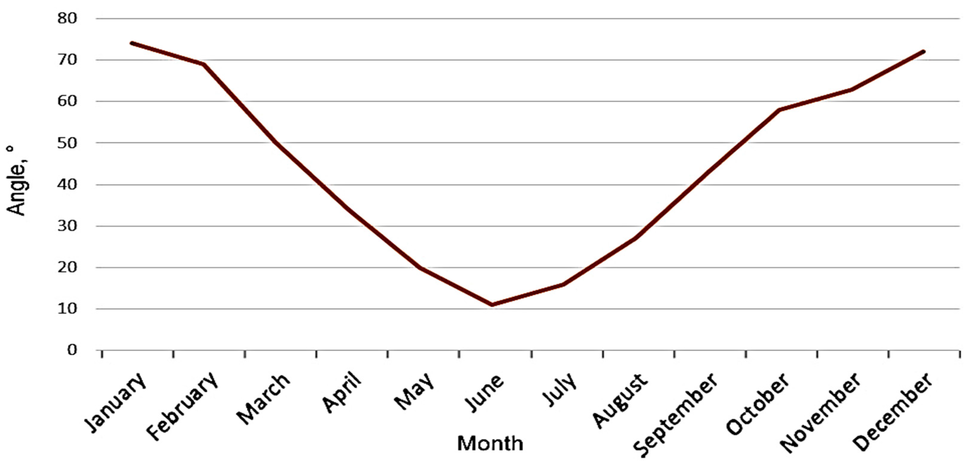
The Sun moves across the sky from east to west. The Sun’s position in the sky is determined by two coordinates, declination and azimuth. Declination is the angle between the line connecting the observer and the Sun and the horizontal surface. The azimuth is the angle between the direction to the Sun and the direction to the south.
It should also be taken into account that the direction to the magnetic south does not always coincide with the direction to the true south. There are true and magnetic poles that do not coincide with each other [32]. Accordingly, there are true and magnetic meridians and, from both of them, it is possible to read off the direction to the desired object. In one case, we deal with the true azimuth; in the other, with a magnetic azimuth. The true azimuth is the angle between the true (geographical) meridian and the direction to the object. The magnetic azimuth is the angle between the magnetic meridian and the direction to a given object. It is clear that the true and magnetic azimuths differ by the same value by which the magnetic meridian differs from the true meridian [33]. This value is called magnetic declination. If the compass needle deviates from the true meridian to the east, the magnetic declination is called east, and if the needle deviates to the west, the declination is called west. Eastern declination is often referred to as “+” (plus) and western declination as “−” (minus). Magnetic declination varies from place to place. Thus, for the Moscow region in Russia, for example, the declination is +6.5… +8.2° and, in general, in the territory of Russia, it varies within more significant limits [34].
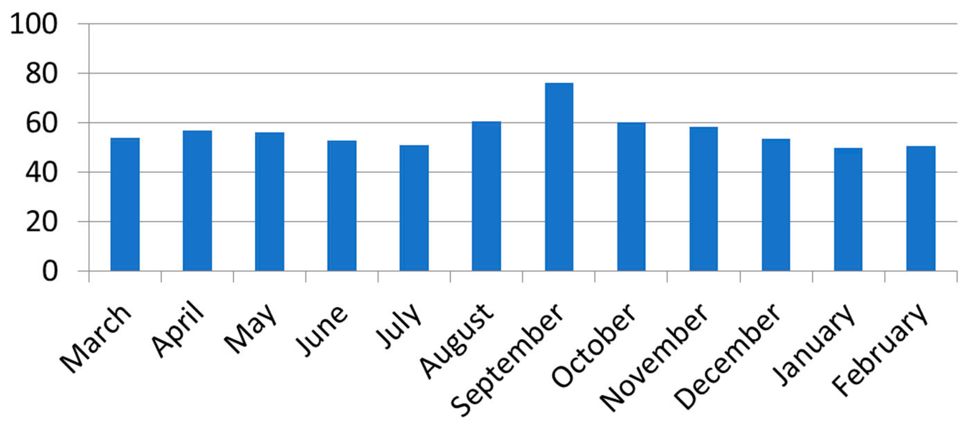
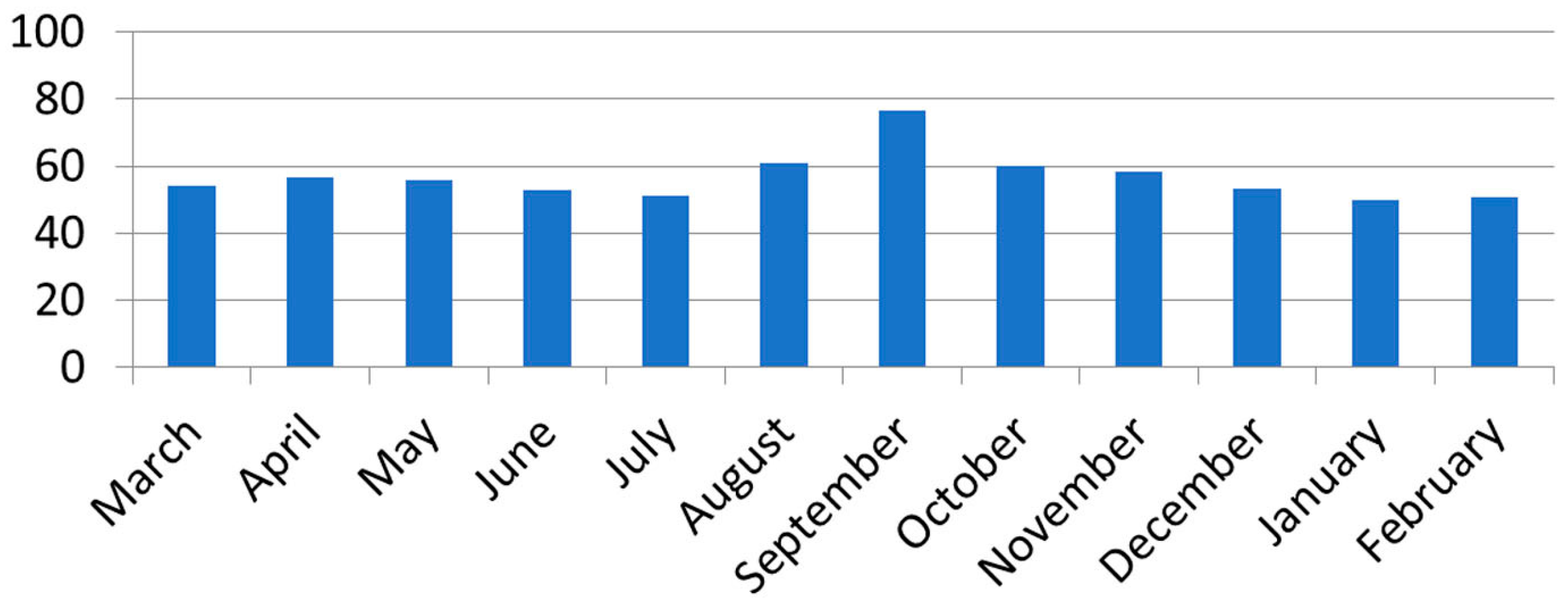
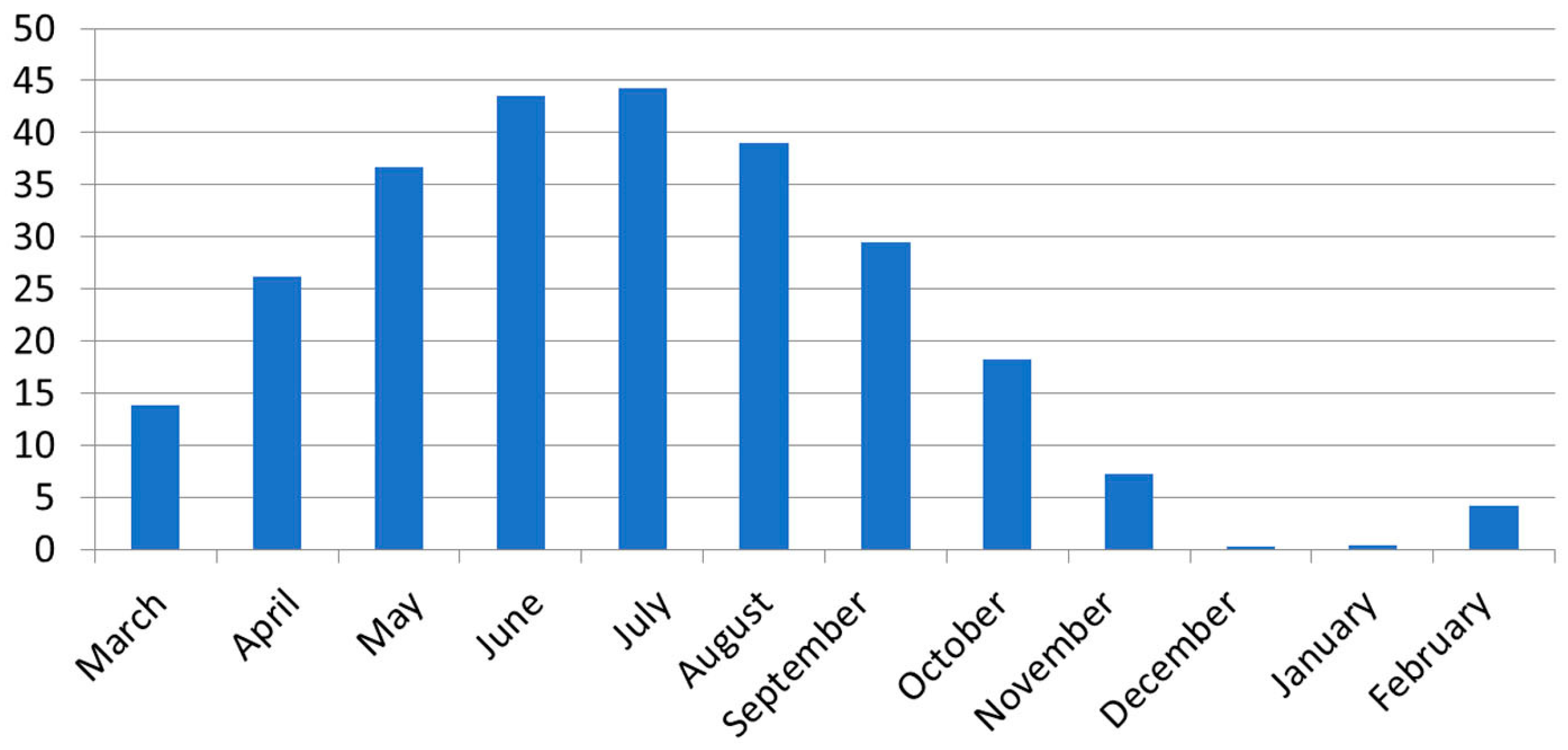
In practice, the solar panels must be oriented at a certain angle to the horizontal surface. Near the equator, the solar panels should be positioned at a very small angle (almost horizontal) in order for the rain to wash the dust and dirt off the PV modules.
Small deviations from this orientation do not play a significant role because, during the day, the Sun moves across the sky from east to west.
To maintain maximum power extraction from the solar panels, special algorithms called maximum power point tracking (MPPT) algorithms are used.
When reviewing the existing MPPT algorithms, it can be noted that there is a large variety of control algorithms. Among them, we can often distinguish:
  • Perturbation and observation algorithm (POA).
  • Adaptive perturbation and observation algorithm (APOA).
  • Algorithm of increasing conductivity (AIC).
  • Algorithm based on fuzzy control logic (ABFCL).
  • Algorithm based on neural networks (ABNN).
  • Fixed voltage algorithm (FVA).
  • Perturbation and observation algorithm (POA).
In the perturbation and observation method, the device changes the input resistance of the inverter by some small amount while changing the voltage on the solar cell (SC). If the power increases, the device continues to change the set parameter until the power no longer increases. This method is widely used, although it has certain disadvantages. Its main advantage is simplicity. Among the disadvantages are: the inability to clearly define the maximum power point (MPP), fluctuations in the operating point around the MPP, a reduced efficiency at a low value of light, and erroneous results when there is a sudden change in the light level.
2.
Adaptive perturbation and observation algorithm (APOA).
The main difference in the adaptive perturbation and observation algorithm (APOA) is that, when the MPP is found, the step by which the given parameter is changed changes depending on the value by which the power has changed. If, at the previous step, the power increased by a larger value than at the current step, then the step of increment will decrease. This allows for a faster and more accurate determination of the MPP.
3.
Algorithm of increasing conductivity (AIC).
In the algorithm of increasing conductivity (AIC), the values of the incremental source voltage and current are measured with a transducer [
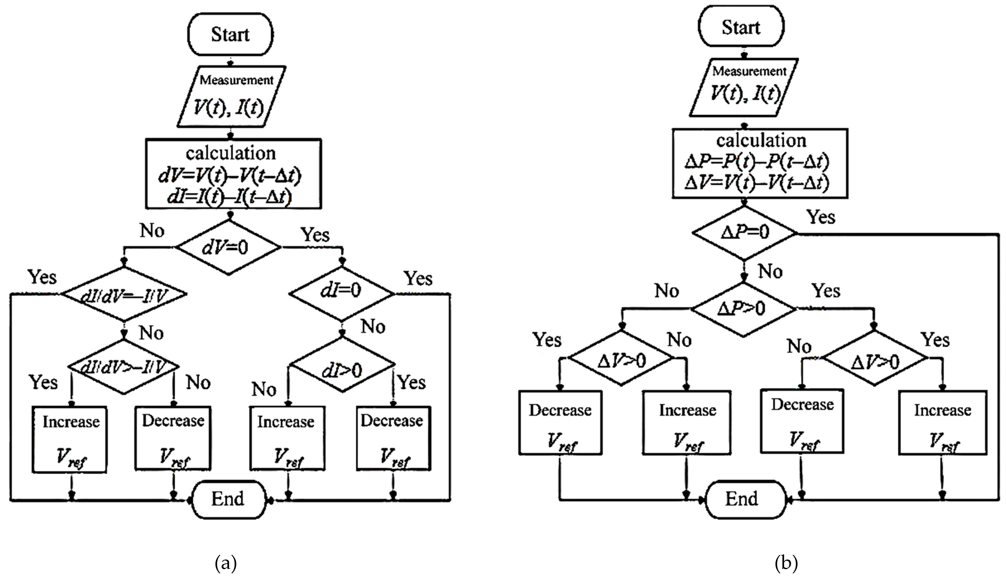
35]. Based on these data, the effect of changes in voltage is predicted. The computational complexity increases, but the speed of tracking changes in ambient conditions also increases. This method uses the increasing conductivity dI/dU to calculate the sign of the change in power with respect to the voltage dP/dU. This calculates the maximum power point and compares the increasing conductivity DI/DU with the solar panel conductivity (I/U). When the condition I/DU = I/U is fulfilled, the output voltage of the SC corresponds to the value of maximum power. The values are then maintained until the illuminance level changes.
As with the APOA method, the main drawback is that this method can easily make mistakes when the light level changes abruptly. Both of these methods are effective at finding the MPP at constant illuminance. However, when the illuminance changes on a slope, the tangent on which the algorithms are based continuously changes with the illuminance as a consequence of changes in the current and voltage not only being due to voltage perturbation. Therefore, the algorithms cannot determine what exactly the change in power is related to [35].
Another disadvantage is that the power value oscillates around the MPP in steady-state mode. This is due to the fact that the control is discrete and that the current and voltage are not constantly at the point of maximum power but fluctuate around it. The main differences in the algorithms AIC and APOA are shown in Figure 8.
Constant voltage algorithm. This method takes advantage of the fact that the ratio between the maximum power point voltage and the CB no-load voltage is approximately linear:
M M P P k 1 · V O C ,
where k 1 is a constant that depends on the characteristics of the photocells and must be determined initially;
M M P P is a voltage corresponding to the maximum power point;
V O C is a no-load voltage of the battery circuit.
To achieve this, we need to compare the values of M M P P and V O C at different levels of light and temperature. In general, the value of this constant ranges from 0.71 to 0.78.
When the value of the constant is determined, the MPP voltage values can be determined by measuring the no-load voltage of the battery. This requires the power converter to be switched off for a moment, which leads to a loss of power. The disadvantage is also the fact that this algorithm is not able to track a constant change in illumination since the voltage measurement process is not continuous. Another disadvantage is that the MPP selected by this method is not valid since the value of the constant is an approximation.
Depending on the application, this algorithm can be used. It is cheap and simple. It does not require a microcontroller (only one voltage sensor is used).
4.
Algorithm based on fuzzy control logic (ABFCL).
Another algorithm that has been gaining popularity lately is the algorithm based on fuzzy control logic (ABFCL), which has become popular in the last decade because it can handle imprecise input data, does not need an exact mathematical model and can handle nonlinearity [36]. Microcontrollers have played no small role in the popularization of fuzzy logic control. Fuzzy logic consists of three stages: phasification, fuzzy inference and defuzzification [4]. Phasification involves the process of converting numerical fuzzy input data into linguistic variables based on the degree of certain sets. Accessory functions are used to bind the score to each linguistic term. The number of affiliation functions used depends on the accuracy of the controller, but typically ranges from 5 to 7.
The input to a fuzzy controller is usually an error, E, and its increment ΔE. The error value can be chosen by the designer, but most often it is chosen as ΔP/ΔV. Thus,
E k = P k P k 1 V k V k 1 ,
Δ E k = E k E k 1 ,
where P k and P k 1 are the power of the photoelectric transducer on the current and previous cycle, respectively;
V k and V k 1 are output voltages of the photoelectric transducer on the current and previous cycles, respectively;
E k and E k 1 are the error on the current and previous measure, respectively;
Δ E k is the incremental error between measures.
The output of a fuzzy converter logic is usually a change in the power converter fill factor, ΔD, or a change in the DC circuit reference voltage, ΔV. The rule base, also known as fuzzy algorithm rules, relates the fuzzy output to fuzzy inputs based on the power converter used [5], which is shown in Table 3.
The last stage of fuzzy logic control is defuzzification. In this step, the output is converted from a linguistic variable to a numeric crisp variable, again using the membership functions. There are various methods for converting linguistic variables into crisp values. The most popular among them is the “center of gravity” method. The advantages of these controllers, in addition to dealing with imprecise input data, a lack of an exact mathematical model and handling nonlinearity, are a fast convergence and minimal fluctuations around the MPP. In addition, they have been shown to work well for step changes in illumination. It is worth noting, however, that no evidence has been found to support the fact that they work well for abrupt changes in illuminance. Another drawback is that their effectiveness depends largely on the skills of the designer, not only in choosing the right error calculation but also in creating an appropriate rule base.
5.
Algorithm based on neural networks (ABNN).
Another method well adapted to microcontrollers is the one based on neural networks. The simplest neural network consists of three layers: input, hidden and output. More complex neural networks are created with hidden layers added. The number of layers and the number of nodes in each layer, as well as the functions used in each layer, vary and depend on user knowledge. Thus, the input variables can be the parameters of the solar panel, its voltage and current, illumination and temperature or a combination of these. The outputs are usually one or more reference signals, such as the duty cycle value or DC link voltage. The performance of the neural network depends on the functions used by the hidden layer and how well the network has been trained [2]. To perform this learning process, pattern data between the inputs and outputs of the neural network are recorded over a long period of time so that the MPP can be accurately tracked [6]. The main disadvantage of this method is the fact that the data required for the training process must be specifically obtained for each PV array and its location because the characteristics of the PV array vary from model to model and the atmospheric conditions vary from location to location. These characteristics also change over time, so the neural network needs to be trained periodically.
6.
Fixed voltage algorithm (FVA).
This algorithm is based on the laws of circuit power and is based on applying a bias voltage from the collector voltage source through a voltage divider with respect to the operating point. The main drawback is the instability of the operating point. The reason for the instability of the operating point is that transistor amplifier stages do not operate under ideal conditions. They are influenced by a variety of factors: ambient temperature, fluctuations in the supply voltage and the presence of electric or magnetic fields in the space (the creation of parasitic inductions). Therefore, it is necessary to stabilize the operating point of the amplifier.
Let us compare the described algorithms in Table 4.
Thus, of the above algorithms, the fuzzy logic algorithm is optimal for the weather station. It has a high efficiency, while its operation is much easier than the algorithm based on neural networks, at a comparable cost. In addition, despite the fact that the implementation of this algorithm is a relatively complex task, it is assumed that, given the specifics of the structure, the implementation will be carried out by a qualified engineer, which, in general, eliminates problems during installation.
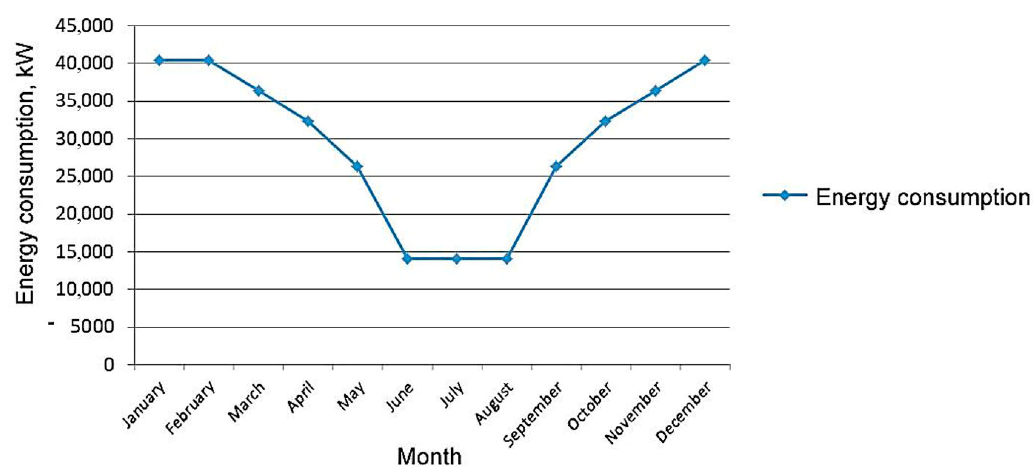
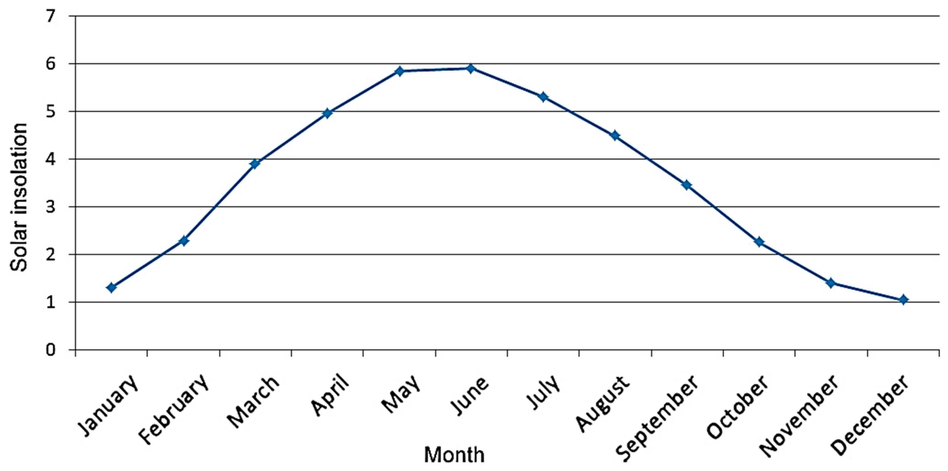
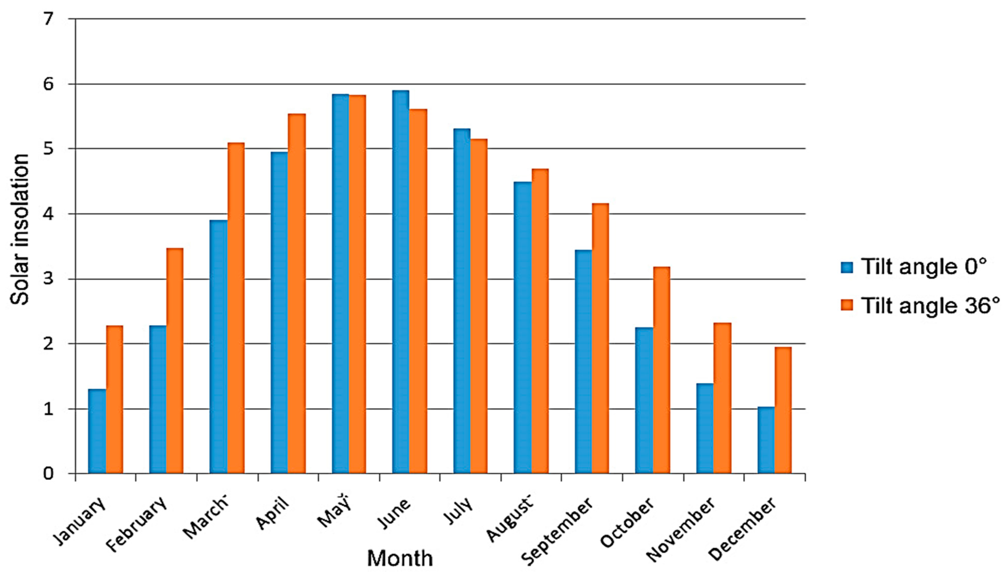
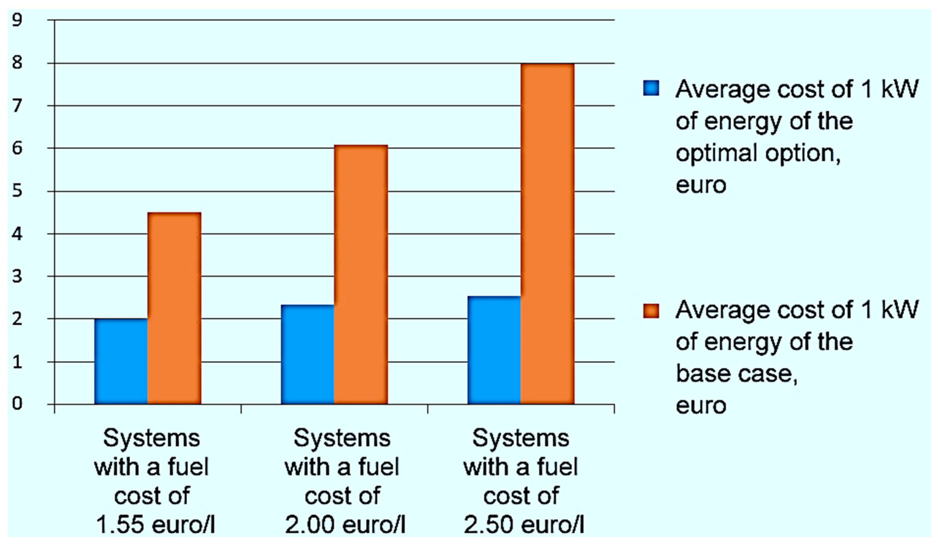
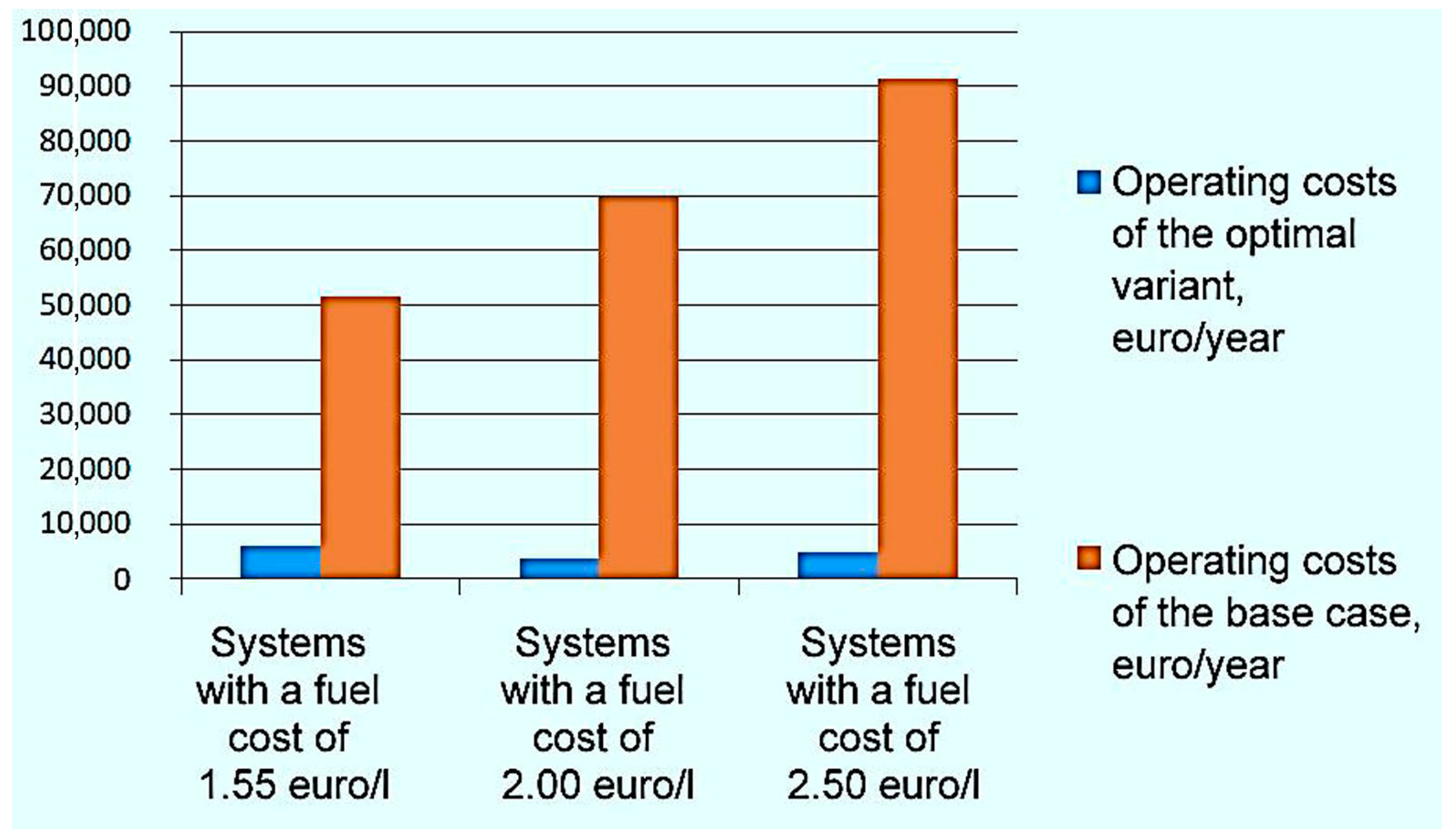
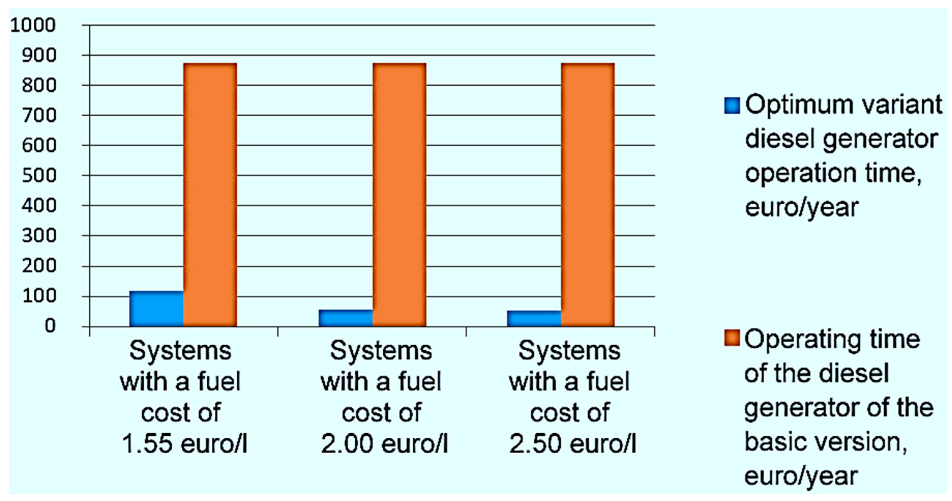
Depending on the spatial location and surrounding conditions, different positioning methods can be selected. In dense urban areas, the use of the static positioning method is more justified due to the lack of sufficient free space and the presence of shading from various objects, despite the fact that the efficiency of this method is significantly (18% or more) lower. When powering remote objects located in places with a low population density and large areas, such as small villages, weather stations and hotels, their use is more reasonable. In addition, when choosing a positioning method, it is important to consider the geographical location and it is desirable to perform calculations to identify the best one for the area (Figure 1, Figure 2 and Figure 3). For example, a comparison of tracking methods relative to Bangladesh [37] showed no significant difference in performance between single-axis and dual-axis positioning. The difference was 4.4%, which is disproportionate to the investment in the two-axis system.

3. Model for Building a Solar Panel Considering the Angle of the Solar Panels

Solar panels are most effective when they face the Sun and their surface is perpendicular to the Sun’s rays. Solar panels are usually placed on the roof or supporting structure in a fixed position and cannot follow the position of the Sun during the day. Therefore, solar panels are usually not at the optimum angle (90 degrees) throughout the day. The angle between the horizontal plane and the solar panel is usually called the tilt angle.
Due to the Earth’s movement around the Sun, there are also seasonal variations. The Sun does not reach the same angle in winter as it does in summer. Ideally, solar panels should be more horizontal in summer than in winter. Therefore, the tilt angle for summer operation is chosen less than for winter operation. If there is no possibility to change the angle twice a year, the panels should be located at the optimum angle, the value of which lies somewhere in the middle between the optimum angles for summer and winter. For each latitude, there is an optimal angle of inclination of the panels. Only for areas near the equator should the solar panels be placed horizontally.
The formula for calculating the capacity of solar panels is
P cp = E p · k · P ins E i n s ,
where Pcp is the power of the solar panels, W;
Ep is the energy consumption, Wh per day;
Eins is the average monthly insolation (from the table) kWh/m2/day;
Pins is the power of insolation on the ground surface in one square meter (1000 W/m2);
k is the coefficient of losses for the charging–discharging of accumulators and the conversion of direct voltage into alternating voltage, usually taken as equal to 1.2… 1.4.
The formula for calculating the energy produced by solar panels is
E v = E i n s · P s p P i n s · k ,
where P s p is the power of the solar panels, W;
E v  is generated by the solar panels, Wh per day;
E i n s  is the average monthly insolation (from the table) kWh/m2/day;
P i n s  is the power of insolation on the ground surface in one square meter (1000 W/m2);
k is the coefficient of losses on the charge–discharge of batteries and the conversion of direct voltage into alternating voltage, usually taken as equal to 1.2.
E v = E i n s · P s p P i n s · η .
Based on the information above, we derive the following formula for calculating the battery output:
E ( s b ) = E ( i n s ) · P ( s b ) P ( i n s ) · η .
where
E ( s b ) is the energy that the solar panel will be able to generate;
E ( i n s ) is a monthly insolation of an area of 1 m2;
P ( s b ) is a panel power rating;
η is the efficiency of the inverter, obtained at the moment of conversion of weak but constant voltage into constant voltage. This value can be excluded from the calculations if one allows the use of low voltage;
P ( i n s ) is the maximum insolation power of an area of 1 m2.
Note that the use of this formula assumes that the insolation and battery output are measured in the same units.
The monthly insolation value is required to estimate the rated capacity of the panels, which is needed in order for the monthly output to be provided. The formula is shown below:
P ( s b ) = P ( i n s ) · E ( s b ) E ( i n s ) · η .
Usually, the optimum slope angle for spring and fall is taken as equal to the latitude value of the terrain. For winter, 10–15 degrees are added to this value and, in summer, 10–15 degrees are subtracted from this value. This is why it is usually recommended to change the angle of slope from summer to winter twice a year. If there is no such opportunity, then the angle of inclination is chosen as approximately equal to the latitude of the terrain.
Thus, an important factor in obtaining maximum electrical power from the solar panel is to calculate the angle of the solar panels and their number needed to cover the needs of all electrical consumers.
Once the approximate amount of electricity required has been determined, one needs to find out what the insolation potential is in a particular area. To achieve this, one needs to obtain information concerning the radiation power of the Sun in one weather or another [38].
During the calculations, it is necessary to consider the angle at which the panels will be located. After all, the performance of the system will directly depend on their rotation to the Sun. The minimum requirement is to calculate the solar capacity for two cases: vertical and horizontal position of photovoltaic modules. If the most precise value is required, the tilt angle should be represented as the sum of the geographic latitude at which the object is located [39]. This value should not be deliberately reduced because, the larger it is, the higher the panels’ yield will be because dust or snow will not start to deposit on them.

3.1. Solar Angle in Winter and Summer

At this stage, let us find the approximate level of performance of the solar panels, i.e., let us calculate exactly how many modules will be needed to create a system with the previously specified capacity.
If we consider that the power of solar radiation is the maximum insolation, we can understand that the performance of the panel refers to the insolation of an area of 1 m2 in the same way as the battery power refers to the power of radiation of the Sun on the surface of our planet under favorable weather conditions. Thus, it is not difficult to find out the level of performance over a 30-day period. To achieve this, one needs to multiply the insolation index for the month by the value that is represented by the ratio of the maximum insolation power to the panel.
A solar panel produces the maximum possible power when the Sun’s rays are perpendicular to it. In this case, it is obvious that maximum efficiency can be achieved if the solar panel is always perpendicular to the Sun. A two-axis positioning system can provide this. However, it is worth bearing in mind that such a system has its disadvantages, which may well outweigh its advantages. Therefore, within the framework of this work, let us consider the advantages and disadvantages of different positioning methods.
The authors were able to identify four methods of positioning solar panels in space:
  • Static positioning.
  • A method taking into account seasonal changes in the slope angle.
  • Single-axis positioning.
  • Two-axis positioning.

3.2. Methods for Positioning Solar Panels in Space

3.2.1. Static Positioning

This method is the easiest to implement. It is mostly used in the private sector, as well as in small commercial and industrial sectors. In this method, the solar panels are fixed in one particular position, most often on roofs or on special ground structures. When using this method, it is especially important to choose the right direction for the location of the solar panel. For example, if the installation site is close to the equator, the battery should be placed as horizontally as possible. If located in the southern hemisphere, the panel should face north; if located in the northern hemisphere, it should face south. One can use information about the location of the Sun during the year to calculate the optimum angle of the panel. For example, we can calculate the optimal angle based on [40]. Let us perform the calculation for Siberia and present it as a graph (Figure 9, Figure 10 and Figure 11).
Based on the data obtained, we can identify the average value of the angle of the Sun’s position. In this case, it is 27.35 degrees.
As one can see from the figures, depending on the geographical location, the optimal angles of the batteries change differently during the year. The advantages of static positioning are that it is a simple and cheap method. It is the most reliable and requires virtually no maintenance. It also does not require a large amount of space; the solar panels can, for example, be mounted on the roof, which is almost impossible with tracking systems. In addition, with a static position, it is quite easy to consider factors such as wind load [41].

3.2.2. With Seasonal Change in the Slope Angle

In order to reduce the losses associated with a suboptimal solar array position, the tilt angle can be adjusted throughout the year. This method is called seasonal tilt adjustment. Then, for Siberia, the solar panel would need to be additionally shifted by −19 °C in winter and by +19 °C in summer (Table 5).
This adjustment will increase the power generation by 5% in winter and summer [41]. On the other hand, at low latitude, the seasonal change in the tilt angle makes no sense (Figure 10).

3.2.3. Single-Axis Positioning

Single-axis trackers are divided into trackers with horizontal (HSAT), tilt (TSAT) and vertical (VSAT) axes of rotation.
Horizontal axis trackers are preferably used in areas close to the equator (Figure 10). The design of such trackers allows for the compact placement of a large number of solar panels. For example, cascades of such panels are placed on a tube, which rotates on its axis and moves all the solar panels on it simultaneously. This is cost-effective and more reliable. Horizontal axial trackers can also be used at higher latitudes by adjusting the slope of the panel [42].
Vertical trackers are used mainly at high latitudes (Figure 11). Unlike horizontal trackers, they are less adapted to dense packing. In addition, when planning, it is worth considering shading to avoid power loss.
Tilted trackers include all trackers with a rotation axis between the vertical and horizontal axis. In certain situations, these trackers can produce more power. However, the tightness of these trackers is even less than that of vertical trackers and depends largely on the tilt angle and the latitude at which they are located.
Single-axis trackers are widespread because they are much cheaper than two-axis trackers and are more reliable and easier to use.

3.2.4. Two-Axis Positioning

This type of tracking has maximum efficiency, allowing the solar panel to follow the Sun exactly at all times. They can be placed at any latitude. In general, they are more versatile. However, they cost significantly more, need more space to be placed, are less reliable and are more difficult to operate.

3.3. Calculation of Solar Cell Power Depending on the Positioning Angle of the Solar Panel

The power of solar panels for stand-alone systems is selected based on the required power output, time of year and geographic location.
The required generated power is determined by the power required by the power consumers that are planned to be used. When calculating, it is worth taking into account the losses in the conversion of DC voltage into AC voltage, charge–discharge of batteries and losses in conductors [43].
Solar radiation is not constant and depends on many factors—the time of year, time of day, weather conditions and geographic location. These factors must also be taken into account when calculating the number of solar panels required. If one plans to use the system year-round, the calculation should take into account the most unfavorable months in terms of solar radiation.
When calculating for the Siberian region, we analyzed statistical data on solar activity over several years. Based on these data, it was possible to determine the averaged actual solar flux power per square meter of the Earth’s surface. These data were obtained from local and international weather services. The statistical data made it possible to predict, with minimal error, the amount of solar energy for our system, which was converted by the solar panels into electric power.
Consider the average daily insolation by month from one of the weather servers for Siberia. The data are given taking into account atmospheric phenomena and are averaged over twenty years.
The unit of insolation in Table 6 is kWh/m2/day.
The angle of inclination of the plane is degrees in relation to the ground (0°—insolation to the horizontal plane, 90°—insolation to the vertical plane, etc.), with the plane oriented to the south (Figure 12).
As can be seen, the most unfavorable month for this region is December, where the daily average insolation on the horizontal ground surface is 0.5 kWh/m2/day and, on the vertical, 1.22 kWh/m2/day. At an angle of inclination of the plane relative to the ground of 70 degrees, the insolation is 1.26 kWh/m2/day, and the optimal angle for December is 74 degrees. The most favorable month is June, where insolation to the horizontal surface is 5.27 kWh/m2/day and the optimal angle of inclination is 11 degrees.
The angle of inclination of the solar panel, when used year-round in a system that consumes on average the same power regardless of the season, should coincide with the optimal angle of inclination of the most unfavorable month in terms of the amount of solar radiation. The optimal angle of inclination for December in Moscow is 74 degrees, so it is worth installing a solar panel as, in other months, the insolation is noticeably greater, and, as a consequence, the production of electricity will be more than enough. Moreover, in winter, at angles of inclination of 70–90 degrees, the solar panel will not accumulate precipitation in the form of snow. If the task is to obtain maximum power from the solar panels throughout the year, it is required to constantly orient the solar panel perpendicular to the Sun [44].

3.4. Wind Energy

Average monthly values of wind speed at a height of 10 m are shown in Table 7.
These results are also confirmed by a study of the wind regime in Siberia [14].
Thus, the prospect of using wind power plants (WPPs) for this area is very low, since wind turbines produce declared power at a wind speed of 8–12 m/s [15], reaching their peak performance at 13–16 m/s. At the same time, the initial speed of the wind turbine is 2.5–3 m/s. Therefore, this type of renewable energy will not be considered further.

3.5. Selection of Equipment for Power Supply of the Weather Station

The choice of equipment is made in order to minimize the average cost per kW of energy produced by the system, so solar panels were selected as the main generators and diesel generators was selected as backup power, while wind turbines were excluded from consideration due to their inefficient use in the area.
Since taking into account the many factors for the rational choice of equipment is a complex mathematical problem, we used the software HOMER to obtain the most accurate optimal results.

3.5.1. Basic System Components

1. Delta bst 450-72 M HC solar panels, the characteristics of which are shown in Table 8.
These photovoltaic modules were chosen because of their good efficiency and peak power, which will reduce the area allocated for the installation of solar panels.
2. SmartWatt eco 5 k inverter. The characteristics are shown in Table 9.
This inverter was chosen because it meets all the stated requirements. It has an mppt controller, and supports parallel operation (up to nine units).
3. OPzV 500 rechargeable batteries. These batteries were chosen because they are maintenance-free, optimized for discharge/recharge operation and have a long service life.
The characteristics are shown in Table 10.
4. Fubag ds 5500 A ES diesel generator. The characteristics are shown in Table 11.
The diesel generator is definitely present in the power supply system as a backup power system. The diesel generator can also be used as a source when the solar panels are not able to generate enough energy to meet the needs of the weather station (overcast days, winter days, at night, etc.).
The generator capacity is enough to independently cover all the load required by the weather station at any time. Also an important parameter is the presence of the generator ATS so that the system without the participation of the operator can turn on the generator if necessary [45].

3.5.2. Additional Factors Affecting Power Generation

When modeling the power supply system, a number of factors must also be taken into account.
1. The location of the solar modules. In this work, it was proposed to install the solar panels on the ground so that there is no natural (trees) and artificial (buildings, masts, various meteorological equipment, etc.) shading, since even a small shading of one of the batteries can significantly affect the total power generated by the system.
Installing the panels on the ground has several advantages. First, they are convenient to maintain. Due to dust or snow pollution, solar panels can lose up to 20% of their efficiency. In addition, the modules installed on the ground, compared with the installation on the roof, will be less susceptible to overheating, and, as a consequence, will be more energy-efficient.
The temperature coefficient, which shows the power loss depending on the heating temperature of the panels. In order to establish the value of these losses, we used the following formula [41]
k T = ( 1.2 · T c 25   ° C ) · k P R ,
where T c is the ambient air temperature;
k P R is the coefficient of power loss due to heating (0.5).
The results of the calculations are summarized in Table 12 and presented in Figure 13.
Thus, we can conclude that there will be no power losses associated with the overheating of the PV modules.

3.5.3. Simulations in HOMER

The goal of the simulation was to design an optimal configuration of the small power system that can fully support the previously described load without power from the grid. The objective function was to minimize the total investment cost (TIC). The variables in this case were the number of: solar panels, batteries and inverters. In this case, the number of diesel generators was taken as 1.
In this case, the target function can be described by the following formula:
T I C = i = 1 n P V N P V i · C P V i + j = 1 n B A T N B A T j · C B A T j + k = 1 n P V N I N V k · C I N V k + l = 1 n D G C D G l
where NPV, NBAT, NINV are the number of elements of each component type, including: solar panels, batteries and inverters, respectively;
CPV, CBAT, CINV, CDG are the total investment cost of each type of component, including: solar panels, batteries, inverters and diesel generator, respectively [46].
Using all the data obtained above, we performed a simulation, the purpose of which was to identify the optimal combination of the proposed equipment based on the use of the system for 20 years [47,48].
Since taking into account all the numerous factors for the rational choice of equipment is a complex mathematical task, we used the software Homer pro (v3.14.2) [20] to obtain the most accurate optimal results. This software is probably the best modern software for the design of electrical networks. Homer pro can simulate the annual operation of a hybrid power system minute by minute. This gives an incredibly high degree of accuracy in estimating the electricity output of the proposed systems. With Homer pro, one can consider different combinations of system parameters simultaneously, as well as determine the most important variables and their best values. Thus, this program was designed to select the best equipment based on the input data. As the initial input data, the previously obtained data on insolation in the area in question were used (Figure 14).
After that, the annual monthly load schedule was filled in. An example of such a schedule is shown in Figure 15.
After that, the composition of the power supply system equipment was selected (Figure 16).
After that, each component of the system was filled according to the previously selected equipment. An example of filling is shown in Figure 17.
The calculated load of the weather station was taken with a factor of 1.1 to account for any unforeseen load, and with a coefficient of random changes in the load schedule of 5%. Thus, the average load of the weather station is 31.55 kW/day.
To ensure that the batteries work for the longest possible period of time, let us set their maximum depth of discharge to 30% (Figure 18).
Since it is not possible to calculate what the exact total cost of diesel fuel will be (including delivery to the selected location), simulations were conducted with three different prices: 1.55 EUR/L (nominal value) and 2 and 2.5 EUR/L.
All obtained systems were compared with the system, which uses only a diesel generator as a source of electricity (Figure 19).
The results of the simulation of the system with a cost of diesel fuel of 1.55 EUR/L are presented in Table 13.
It follows from the results that the renewable energy system will cost 55.75% less over a 20-year period, despite the fact that the initial capital for the system with RES is 37.5 times higher than in the basic system (Figure 20 and Figure 21). It is also worth noting that the system uses four single-phase inverters, selected earlier, in parallel mode. The use of this option compared to the use of a more powerful inverter is due to:
  • A lack of a single phase for more than 7.5 kW.
  • The selected object has no three-phase load and the presence of mainly one powerful consumer at any given time.
  • As a consequence of 2, the asymmetry of currents and voltages in the system.
  • The possibility of parallel operation of single-phase inverters.
  • Not much difference in cost between these options.
  • When using two or more inverters, if one of them fails, the others will remain in operation; as a consequence, the reliability of the system is higher.
The results of the simulation of the system with a cost of diesel fuel of 2 EUR/L are presented in Table 14.
For a given fuel cost, a system with RES would cost 61.6% less. At the same time, the initial investment also increases (51.6 times), which is associated with an increased number of solar modules, batteries and inverters. One can also see that the running time of the diesel generator has been reduced by two times, while fuel costs have increased by only 39% (Figure 22 and Figure 23). The cost of the basic version compared to the previous one has increased dramatically. The autonomous operation time has also increased. The payback period of the system has decreased.
The results of the simulation of the system with a cost of diesel fuel of 2.5 EUR/L are presented in Table 15.
At the given cost of diesel fuel, the total cost of the optimal variant is 68.4% cheaper than the base case (Figure 24). At the same time, the initial investment is 53.6 times more than in the base case, which is a little more than in the variant with a cost of diesel of 2.5 EUR/L, although the cost of fuel increased by 33.3% (Figure 25, Figure 26 and Figure 27). The payback period is 5.55 years.
Thus, a simulation was performed in order to establish the most optimal configuration of selected components at three different diesel fuel prices.
As a result, data were obtained on the value of the initial investment, the annual operating costs and the total cost of the systems and the payback period of the systems. The baseline and optimal options were compared.

4. Conclusions

In this work, we analyzed twenty years of information on solar activity based on statistical data for the Siberian region. Based on these data, we were able to determine the average actual solar flux power per square meter of the Earth’s surface. These data were obtained from local and international weather services. The statistical data made it possible to predict, with minimal error, the amount of solar energy for our system, which was converted by the solar panels into electric power.
We analyzed the data and obtained a picture of the averaging of daily insolation by months from one of the servers of weather services for Siberia. The data are given taking into account atmospheric phenomena and are averaged over twenty years.
We developed a model of an autonomous power supply system using renewable energy sources for a decentralized facility located in Siberia in the form of a weather station.
Based on the data obtained, modern components, available on the Russian market, were selected to create a power supply system. The consumer load schedule is presented and the average annual power consumption of meteorological stations was determined. Climatic conditions of the selected area were analyzed. Prospective renewable energy sources were selected. Various factors associated with energy losses in the use of renewable energy sources were considered. The conditions and location of the system were stipulated. The main components of the energy supply system were selected. A simulation was performed in order to establish the most optimal configuration of the selected components at three different diesel fuel prices.
An analysis of the current state of the market of renewable energy sources was carried out. The factors influencing the efficiency of systems with renewable energy sources were analyzed. As a result, the results of the technical and economic analysis of data on the value of the initial investment, operating annual costs and payback period of the autonomous energy systems were obtained. The basic and optimal options were compared and the most effective of them were identified.
The choice of the most effective algorithm for use at a weather station was made. The effective placement of solar panels was also calculated, and the conditions of placement depending on the territorial location and various environmental conditions were determined. A simulation of the power supply system of the weather station, consisting of solar panels, batteries and inverters, was conducted. As a result, a practical example of applying the method of selecting the optimal composition of equipment for the hybrid power supply system of the weather station, geographically located in Siberia, with different configurations of equipment was considered. In numerical terms, it was possible to reduce the cost of power equipment operation by more than 60% with a fairly low payback period of 5.5 years and increase the reliability of the power system, which is very important for autonomous power systems of northern weather stations.

Author Contributions

Conceptualization, N.V.M. and B.V.M.; methodology, R.V.K.; software, R.V.K.; validation, V.Y.K., V.A.K. and V.T.; formal analysis, V.Y.K. and E.V.V.; investigation, Y.A.T.; resources, V.A.K. and V.T.; data curation, Y.A.T.; writing—original draft preparation, N.V.M. and B.V.M.; writing—review and editing, B.V.M. and N.V.M.; visualization, E.V.V. and R.V.K. All authors have read and agreed to the published version of the manuscript.

Funding

This research received no external funding.

Data Availability Statement

The data presented in this study are available from the corresponding authors upon reasonable request.

Conflicts of Interest

The authors declare no conflict of interest.

References

  1. Zahraoui, Y.; Alhamrouni, I.; Mekhilef, S.; Basir Khan, M.R.; Seyedmahmoudian, M.; Stojcevski, A.; Horan, B. Energy Management System in Microgrids: A Comprehensive Review. Sustainability 2021, 13, 10492. [Google Scholar] [CrossRef]
  2. Tailor, R.; Bena, L.; Conka, Z.; Kolcun, M. Design of Management Systems for Smart Grid. In Proceedings of the 2021 Selected Issues of Electrical Engineering and Electronics (WZEE), Rzeszow, Poland, 13–15 September 2021. [Google Scholar]
  3. Mohseni, S.; Brent, A.C.; Burmester, D. Off-Grid Multi-Carrier Microgrid Design Optimisation: The Case of Rakiura-Stewart Island, Aotearoa-New Zealand. Energies 2021, 14, 6522. [Google Scholar] [CrossRef]
  4. Climate Action. Available online: https://ec.europa.eu/clima/eu-action/international-action-climate-change/climatenegotiations/paris-agreement_en (accessed on 18 October 2021).
  5. Min, H.S.; Wagh, S.; Kadier, A.; Gondal, I.A.; Azim, N.A.P.B.A.; Mishra, M.K. Edition: 7 Chapter: Renewable Energy Technologies; Min, H.S., Ed.; Ideal International E-Publication Pvt. Ltd.: Indore, India, 2018. [Google Scholar]
  6. Sustainable Developments. Available online: https://www.un.org/sustainabledevelopment/energy/ (accessed on 18 October 2021).
  7. Yelemessov, K.; Sabirova, L.B.; Martyushev, N.V.; Malozyomov, B.V.; Bakhmagambetova, G.B.; Atanova, O.V. Modeling and Model Verification of the Stress-Strain State of Reinforced Polymer Concrete. Materials 2023, 16, 3494. [Google Scholar] [CrossRef] [PubMed]
  8. Jurasz, J.; Canales, F.A.; Kies, A.; Guezgouz, M.; Beluco, A. A review on the complementarity of renewable energy sources: Concept, metrics, application and future research directions. Sol. Energy 2020, 195, 703–724. [Google Scholar] [CrossRef]
  9. Feddaoui, O.; Toufouti, R.; Labed, D.; Meziane, S. Control of an Isolated Microgrid Including Renewable Energy Resources. Serb. J. Electr. Eng. 2020, 17, 297–312. [Google Scholar] [CrossRef]
  10. Schurov, N.I.; Myatezh, S.V.; Myatezh, A.V.; Malozyomov, B.V.; Shtang, A.A. Inactive power detection in AC network. Int. J. Electr. Comput. Eng. 2021, 11, 966–974. [Google Scholar] [CrossRef]
  11. John Bhatti, H.; Danilovic, M. Making the World More Sustainable: Enabling Localized Energy Generation and Distribution on Decentralized Smart Grid Systems. World J. Eng. Technol. 2018, 6, 350–382. [Google Scholar] [CrossRef] [Green Version]
  12. Deng, Z.; Xiao, J.; Zhang, S.; Xie, Y.; Rong, Y.; Zhou, Y. Economic feasibility of large-scale hydro-solar hybrid power including long distance transmission. Glob. Energy Interconnect. 2019, 2, 290–299. [Google Scholar] [CrossRef]
  13. Shchurov, N.I.; Myatezh, S.V.; Malozyomov, B.V.; Shtang, A.A.; Martyushev, N.V.; Klyuev, R.V.; Dedov, S.I. Determination of Inactive Powers in a Single-Phase AC Network. Energies 2021, 14, 4814. [Google Scholar] [CrossRef]
  14. Li, H.; Liu, P.; Guo, S.; Ming, B.; Cheng, L.; Yang, Z. Long-term complementary operation of a large-scale hydro-photovoltaic hybrid power plant using explicit stochastic optimization. Appl. Energy 2019, 238, 863–875. [Google Scholar] [CrossRef]
  15. Ausfelder, F.; Beilmann, C.; Bertau, M.; Bräuninger, S.; Heinzel, A.; Hoer, R.; Koch, W.; Mahlendorf, F.; Metzelthin, A.; Peuckert, M.; et al. Energy Storage as Part of a SecureEnergy Supply. ChemBioEng Rev. 2017, 4, 144–210. [Google Scholar] [CrossRef] [Green Version]
  16. Li, F.F.; Qiu, J. Multi-objective optimization for integrated hydro-photovoltaic power system. Appl. Energy 2016, 167, 377–384. [Google Scholar] [CrossRef]
  17. Malozyomov, B.V.; Martyushev, N.V.; Sorokova, S.N.; Efremenkov, E.A.; Qi, M. Mathematical Modeling of Mechanical Forces and Power Balance in Electromechanical Energy Converter. Mathematics 2023, 11, 2394. [Google Scholar] [CrossRef]
  18. Lawan, S.M.; Abidin, W.A.W.Z. A Review of Hybrid Renewable Energy Systems Based on Wind and Solar Energy: Modeling, Design and Optimization; Wind Solar Hybrid Renewable Energy System: London, UK, 2020; 21p.
  19. Burger, C.; Froggatt, A.; Mitchell, C.; Weinmann, J. Decentralized Energy: A Global Game Changer; Ubiquity Press: Berkeley, CA, USA, 2020. [Google Scholar]
  20. Mohseni, S.; Brent, A.C.; Burmester, D. Community Resilience-Oriented Optimal Micro-Grid Capacity Expansion Planning: The Case of Totarabank Eco-Village, New Zealand. Energies 2020, 13, 3970. [Google Scholar] [CrossRef]
  21. Matrenin, P.; Safaraliev, M.; Dmitriev, S.; Kokin, S.; Ghulomzoda, A.; Mitrofanov, S. Medium-term load forecasting in isolated power systems based on ensemble machine learning models. Energy Rep. 2022, 8, 612–618. [Google Scholar] [CrossRef]
  22. Malozyomov, B.V.; Martyushev, N.V.; Kukartsev, V.A.; Kukartsev, V.V.; Tynchenko, S.V.; Klyuev, R.V.; Zagorodnii, N.A.; Tynchenko, Y.A. Study of Supercapacitors Built in the Start-Up System of the Main Diesel Locomotive. Energies 2023, 16, 3909. [Google Scholar] [CrossRef]
  23. Kirgizov, A.K.; Dmitriev, S.A.; Safaraliev, M.K.; Pavlyuchenko, D.A.; Ghulomzoda, A.H.; Ahyoev, J.S. Expert system application for reactive power compensation in isolated electric power systems. Int. J. Electr. Comput. Eng. 2021, 11, 3682–3691. [Google Scholar] [CrossRef]
  24. Asanov, M.S.; Safaraliev, M.K.; Zhabudaev, T.Z.; Asanova, S.M.; Kokin, S.E.; Dmitriev, S.A.; Obozov, A.J.; Ghulomzoda, A.H. An algorithm for calculation and selection of micro hydropower plant taking into account hydro-logical parameters of small watercourses mountain rivers of Central Asia. Int. J. Hydrog. Energy 2021, 46, 37109–37119. [Google Scholar] [CrossRef]
  25. Jurasz, J.; Dabek, P.B.; Kazmierczak, B.; Kies, A.; Wdowikowski, M. Large scale complementary solar and wind energy sources coupled with pumped-storage hydroelectricity for Lower Silesia (Poland). Energy 2018, 161, 183–192. [Google Scholar] [CrossRef]
  26. Yang, Z.; Liu, P.; Cheng, L.; Wang, H.; Ming, B.; Gong, W. Deriving operating rules for a large-scale hydro-photovoltaic power system using implicit stochastic optimization. J. Clean. Prod. 2018, 195, 562–572. [Google Scholar] [CrossRef]
  27. Martyushev, N.V.; Malozyomov, B.V.; Khalikov, I.H.; Kukartsev, V.A.; Kukartsev, V.V.; Tynchenko, V.S.; Tynchenko, Y.A.; Qi, M. Review of Methods for Improving the Energy Efficiency of Electrified Ground Transport by Optimizing Battery Consumption. Energies 2023, 16, 729. [Google Scholar] [CrossRef]
  28. Kougias, I.; Szabo, S.; Monforti-Ferrario, F.; Huld, T.; Bódis, K. A methodology for optimization of the complementarity between small-hydropower plants and solar PV systems. Renew. Energy 2016, 87, 1023–1030. [Google Scholar]
  29. Parastegari, M.; Hooshmand, R.A.; Khodabakhshian, A.; Zare, A.H. Joint operation of wind farm, photovoltaic, pump-storage and energy storage devices in energy and reserve markets. Int. J. Electr. Power Energy Syst. 2015, 64, 275–284. [Google Scholar] [CrossRef]
  30. Jure, M.; Zvonimir, G. Feasibility of the green energy production by hybrid solar + hydro power system in Europe and similar climate areas. Renew. Sustain. Energy Rev. 2010, 14, 1580–1590. [Google Scholar]
  31. Dinglin, L.; Yingjie, C.; Kun, Z.; Ming, Z. Economic evaluation of wind-powered pumped storage system. Syst. Eng. Procedia 2012, 4, 107–115. [Google Scholar] [CrossRef] [Green Version]
  32. Bekirov, E.A.; Strizhakov, K. Optimization of load distribution modes in a combined system with renewable energy sources. Motrol 2012, 1, 146–150. [Google Scholar]
  33. Martyushev, N.V.; Malozyomov, B.V.; Sorokova, S.N.; Efremenkov, E.A.; Qi, M. Mathematical Modeling of the State of the Battery of Cargo Electric Vehicles. Mathematics 2023, 11, 536. [Google Scholar] [CrossRef]
  34. Ma, T.; Lashway, C.R.; Song, Y.; Mohammed, O. Optimal renewable energy farm and energy storage sizing method for future hybrid power system. In Proceedings of the 2014 17th International Conference on Electrical Machines and Systems (ICEMS), Hangzhou, China, 22–25 October 2014; pp. 2827–2832. [Google Scholar]
  35. Shahirinia, A.H.; Tafreshi, S.M.M.; Gastaj, A.H.; Moghaddomjoo, A.R. Optimal sizing of hybrid power system using genetic algorithm. In Proceedings of the 2005 International Conference on Future Power Systems, Amsterdam, The Netherlands, 18 November 2005; pp. 1–6. [Google Scholar]
  36. Shchurov, N.I.; Dedov, S.I.; Malozyomov, B.V.; Shtang, A.A.; Martyushev, N.V.; Klyuev, R.V.; Andriashin, S.N. Degradation of Lithium-Ion Batteries in an Electric Transport Complex. Energies 2021, 14, 8072. [Google Scholar] [CrossRef]
  37. Gang, L.; Heqing, S.; Dragan, R. Power generation cost minimization of the grid-connected hybrid renewable energy system through optimal sizing using the modified seagull optimization technique. Energy Rep. 2020, 6, 3365–3376. [Google Scholar]
  38. Ma, T.; Mohammed, O. Economic analysis of real-time large scale PEVs network power flow control algorithm with the consideration of V2G services. In Proceedings of the 2013 IEEE Industry Applications Society Annual Meeting, Lake Buena Vista, FL, USA, 6–11 October 2013; pp. 1–8. [Google Scholar]
  39. Chen, S.X.; Gooi, H.B.; Wang, M.Q. Sizing of Energy Storage for Microgrids. IEEE Trans. Smart Grid 2012, 3, 142–151. [Google Scholar] [CrossRef]
  40. Xu, L.; Ruan, X.; Mao, C.; Zhang, B.; Luo, Y. An Improved Optimal Sizing Method for Wind-Solar-Battery Hybrid Power System. IEEE Trans. Sustain. Energy 2013, 4, 774–785. [Google Scholar]
  41. Safaraliev, M.K.; Odinaev, I.N.; Ahyoev, J.S.; Rasulzoda, K.N.; Otashbekov, R.A. Energy Potential Estimation of the Region’s Solar Radiation Using a Solar Tracker. Appl. Sol. Energy 2020, 56, 270–275. [Google Scholar] [CrossRef]
  42. Shakirov, V.A.; Artemyev, A.Y. The choice of a site for the placement of a wind power plant using computer modeling of terrain and wind flow. Bull. Irkutsk State Tech. Univ. 2017, 21, 133–143. [Google Scholar] [CrossRef]
  43. Manusov, V.; Nazarov, M. Energy Consumption Conditions Optimization of the Autonomous System Based on Carbon-Free Energy. In Proceedings of the 2020 Ural Smart Energy Conference (USEC), Ekaterinburg, Russia, 13–15 November 2020; pp. 93–96. [Google Scholar]
  44. Isametova, M.E.; Nussipali, R.; Martyushev, N.V.; Malozyomov, B.V.; Efremenkov, E.A.; Isametov, A. Mathematical Modeling of the Reliability of Polymer Composite Materials. Mathematics 2022, 10, 3978. [Google Scholar] [CrossRef]
  45. Matrenin, P.; Safaraliev, M.; Dmitriev, S.; Kokin, S.; Eshchanov, B.; Rusina, A. Adaptive ensemble models for medium-term forecasting of water inflow when planning electricity generation under climate change. Energy Rep. 2022, 8, 439–447. [Google Scholar] [CrossRef]
  46. Ghulomzoda, A.; Gulakhmadov, A.; Fishov, A.; Safaraliev, M.; Chen, X.; Rasulzoda, K.; Gulyamov, K.; Ahyoev, J. Recloser-Based Decentralized Control of the Grid with Distributed Generation in the Lahsh District of the Rasht Grid in Tajikistan, Central Asia. Energies 2020, 13, 3673. [Google Scholar] [CrossRef]
  47. Malozyomov, B.V.; Golik, V.I.; Brigida, V.; Kukartsev, V.V.; Tynchenko, Y.A.; Boyko, A.A.; Tynchenko, S.V. Substantiation of Drilling Parameters for Undermined Drainage Boreholes for Increasing Methane Production from Unconventional Coal-Gas Collectors. Energies 2023, 16, 4276. [Google Scholar] [CrossRef]
  48. Martyushev, N.V.; Malozyomov, B.V.; Sorokova, S.N.; Efremenkov, E.A.; Qi, M. Mathematical Modeling the Performance of an Electric Vehicle Considering Various Driving Cycles. Mathematics 2023, 11, 2586. [Google Scholar] [CrossRef]
Figure 1. Meteorological station.
Energies 16 05046 g001
Figure 2. Graph of the average monthly temperature in Siberia (blue line) and average daily temperature (red line).
Energies 16 05046 g002
Figure 3. December daily load schedule of the weather station.
Energies 16 05046 g003
Figure 4. June daily load schedule of the weather station.
Energies 16 05046 g004
Figure 5. Annual load of the weather station.
Energies 16 05046 g005
Figure 6. Solar insolation on the horizontal surface.
Energies 16 05046 g006
Figure 7. Solar insolation as a function of tilt angle.
Energies 16 05046 g007
Figure 8. Control algorithms: (a)—AIC; (b)—APOA.
Energies 16 05046 g008
Figure 9. Angle of the Sun during the year in Siberia.
Energies 16 05046 g009
Figure 10. Angle of the Sun during the year in Singapore.
Energies 16 05046 g010
Figure 11. Angle of the Sun during the year in Narvik.
Energies 16 05046 g011
Figure 12. Curve of average daily insolation by months from one of the servers of weather services for Siberia.
Energies 16 05046 g012
Figure 13. Power losses as a function of average monthly ambient air temperature.
Energies 16 05046 g013
Figure 14. Data on solar insolation.
Energies 16 05046 g014
Figure 15. Graph of the annual load of the facility.
Energies 16 05046 g015
Figure 16. Equipment composition of the facility.
Energies 16 05046 g016
Figure 17. Parameters of the solar panel.
Energies 16 05046 g017
Figure 18. State of charge of the battery during the year.
Energies 16 05046 g018
Figure 19. Consumption of diesel generator during the year.
Energies 16 05046 g019
Figure 20. Battery charge status during the year.
Energies 16 05046 g020
Figure 21. Consumption of diesel generator during the year.
Energies 16 05046 g021
Figure 22. State of charge of the battery pack during the year.
Energies 16 05046 g022
Figure 23. Consumption of diesel generator during the year.
Energies 16 05046 g023
Figure 24. Comparison of the net present value of the systems.
Energies 16 05046 g024
Figure 25. Comparison of the average cost of 1 kW of energy of the systems.
Energies 16 05046 g025
Figure 26. Comparison of system operating costs.
Energies 16 05046 g026
Figure 27. Comparison of operating times of diesel generator systems.
Energies 16 05046 g027
Table 1. Load of the weather station.
TypeNamePower, WattQuantity, pcs.
Household loadLamps88
TV601
Refrigerator1501
Kettle10001
Microwave10501
Electric stove20001
Computer3501
Washing machine21001
Iron10001
Vacuum cleaner10001
Meteorological equipmentThe Cloudmaker30 (260)1
Anemorumbometer251
Precipitator 251
Actual weather sensor6 (36)1
Psychometer301
Water and heatingElectric boiler53501
Circulation pump601
Water heater2501
Table 2. Average monthly insolation depending on the angle of inclination of solar panels.
Tilt Angle, gr.36°51°66°90°
January1.32.292.522.612.46
February2.293.483.73.733.39
March3.95.15.195.014.22
April4.965.555.324.843.61
May5.855.835.334.633.11
June5.95.625.064.332.85
July5.315.154.684.052.74
August4.494.74.43.922.8
September3.454.164.13.833.01
October2.253.193.313.252.8
November1.42.322.522.582.4
December1.041.952.172.262.16
Average annual3.514.114.023.752.96
Table 3. Table of fuzzy rules.
CurrentSunlight
SmallMediumLarge
SmallSmallMediumLarge
MediumSmallSmallMedium
LargeSmallSmallSmall
Table 4. Comparison of algorithms.
TypeDifficulty of ImplementationDifficulty of OperationCostKPI
Perturbation and observation algorithm (POA)SimpleSimpleMedium90.2
Adaptive perturbation and observation algorithm (APOA)SimpleSimpleMedium90.2
Algorithm of increasing conductivity (AIC)MediumSimpleMedium93.1
Fixed voltage algorithm (FVA)SimpleSimpleCheap92.9
Algorithm based on fuzzy control logic (ABFCL)HardMediumExpensive99%
Algorithm based on neural networks (ABNN)HardHardExpensive99%
Table 5. Values of Sun position angles by season relative to the optimum angle.
SeasonSpringSummerAutumnWinter
Tilt angle3.27918.52−2.337−19.46
Table 6. Average daily insolation by month from one of the weather service servers for Siberia.
The Value of the Tilt Angle JanuaryFebruaryMarchAprilMayJuneJulyAugustSeptemberOctoberNovemberDecemberInsolation during the Year kWh/m2/day
0.500.812.813.875.135.275.144.302.631.491.560.752.92
36°1.081.463.784.345.124.975.004.573.222.202.551.513.45
52°1.201.583.824.164.704.514.534.313.172.272.701.663.18
68°1.261.623.673.794.183.954.003.852.972.242.711.723.06
84°1.221.533.193.073.212.993.053.082.512.022.501.652.68
Optimal angle74.069.050.034.020.011.016.027.043.058.063.072.046.3
Table 7. Average monthly wind speed.
MonthWind Speed, m/s
January1.36
February1.6
March2.06
April2.52
May2.34
June1.84
July1.57
August1.56
September1.75
October1.69
November1.51
December1.35
Annual average1.76
Table 8. Characteristics of the solar panel.
NameDelta bst 450-72 M HC
TechnologyMonocrystal
Quality categoryGrade A
Peak power, watts450
Nominal voltage, V24
Voltage at maximum power point, V43.9
Current at maximum power point, A10.2
Short-circuit current, A10.57
Efficiency, %20.42
Loss of capacity over 10 years, %10
Table 9. Characteristics of the inverter.
NameSmartWatt eco 5 k
Rated power, kW5
Peak power, kW10
Frequency, Hz50
Operating frequency range, Hz46–53
The form of the output outfitPure sine wave
Battery voltage, V48
Controller typeMPPT
Operating temperature, °C0 to 50
Efficiency, %92
Service life, years12
Table 10. Battery characteristics.
NameOPzV 500
TechnologyGEL (Lead Acid)
Voltage, V2
Capacity, Ah500
Service life, years20
Table 11. Characteristics of the diesel generator.
NameFubag ds 5500 A ES
Nominal voltage, V230
Constant load, kW5
Peak load, kW5.5
Nominal fuel consumption, L2.5
Fuel consumption at 75% load, L/h2.09
Startup systemManual/auto start
Table 12. Power losses as a function of average monthly ambient air temperature.
MonthAmbient Temperature, °CTemperature, Taking into Account the Installation Factor, °CPower Loss, %
January−21.79−26.148−25.574
February−18.28−21.936−23.468
March−10.82−12.984−18.992
April−1.02−1.224−13.112
May7.289.852−8.132
June14.5717.484−3.758
July17.4220.904−2.048
August14.6717.604−3.698
September6.828.184−8.408
October−1.6−1.92−13.46
November−11.51−13.812−19.406
December−18.92−22.704−23.852
Table 13. Simulation results of the system with a cost of diesel fuel of 1.55 EUR/L.
IndicatorsOptimal VariantBasic Version
Installed capacity of solar panels, kW19.8-
Installed capacity of diesel generator, kW55
Number of batteries, pcs.72-
Number of inverters, pcs.4-
Net present value, euros65,719148,526
Average cost of 1 kW of energy, EUR0.250.89
Operating costs, EUR/year871.197361.9
Initial investment, EUR48,2961288.6
Total amount of fuel consumed by diesel generator, L1157
Operating time of diesel generator, hours938
System operating time from rechargeable batteries, hours16.8-
Payback period of the relative base case, years7.4
Table 14. Simulation results of the system with a cost of diesel fuel of 2 EUR/L.
IndicatorsOptimal VariantBasic Version
Installed capacity of solar panels, kW29.25-
Installed capacity of diesel generator, kW55
Number of batteries, pcs.96-
Number of inverters, pcs.6-
Net present value, EUR76,915.8200,433.7
Average cost of 1 kW of energy, EUR0.250.89
Operating costs, EUR/year521.949957.28
Initial investment, EUR66,476.81288.5
Total amount of fuel consumed by diesel generator, l5578651
Operating time of diesel generator, hours4888760
System operating time from rechargeable batteries, hours22.3-
Payback period of the relative base case, years6.93-
Table 15. Simulation results of the system with a cost of diesel fuel of 2.5 EUR/L.
IndicatorsOptimal VariantBasic Version
Installed capacity of solar panels, kW31.5-
Installed capacity of diesel generator, kW55
Number of batteries, pcs.96-
Number of inverters, pcs.7-
Net present value, EUR82,863.2262,228.1
Average cost of 1 kW of energy, EUR0.250.89
Operating costs, EUR/year691.713,046.9
Initial investment, EUR4,832,06090,200
Total amount of fuel consumed by diesel generator, L5268651
Operating time of diesel generator, hours4628760
System operating time from rechargeable batteries, hours22.3-
Payback period of the relative base case, years5.55-
Disclaimer/Publisher’s Note: The statements, opinions and data contained in all publications are solely those of the individual author(s) and contributor(s) and not of MDPI and/or the editor(s). MDPI and/or the editor(s) disclaim responsibility for any injury to people or property resulting from any ideas, methods, instructions or products referred to in the content.

