Abstract
Sustainable greenhouses have gained relevance in recent years due to their potential to reduce the carbon footprint of the agricultural sector by being integrated with renewable systems, contributing to the decarbonization of energy. Although solar technologies tend to be more accessible to cover the system’s energy demands, greenhouses are subject to installation area restrictions, limiting their energy potential. This research evaluates the energy advantages of hybridizing solar thermal collector fields with photovoltaic module fields to cover a greenhouse’s cooling and heating demands. For this purpose, the solar thermal field and the photovoltaic solar system were simulated with TRNSYS and MATLAB, respectively, while a method was developed to simulate the performance of a single-effect absorption chiller that was validated using the temperature measurements of a chiller in operation. The results show that the general method maintains differences between measurements and simulation smaller than with set temperatures between 5.5 and 12 degrees Celsius. The hybrid system, with an air-to-water chiller as the main machine and absorption chiller, reached a solar fraction of 0.85 and a fractional energy saving of . This represents a reduction in area concerning an individual solar thermal system. This research highlights that the solar hybrid configuration reduces fossil energy consumption by improving the global efficiency of energy conversion, thereby reducing the area of the solar field.
1. Introduction
The goal of global decarbonization of electricity by 2050 is linked to the integration of renewable energy to replace fossil energy sources. In turn, to achieve sustainable growth, it is necessary to reduce electricity consumption without affecting energy supply [1]. For this reason, the International Energy Agency (IEA), as well as international agreements, focus their efforts on the development of new technologies to reduce electricity consumption [2]. One focus of such efforts is on cooling processes, with strategies that seek to develop more efficient chillers and the integration of renewable energy sources such as solar photovoltaic (PV) and solar thermal (ST) energy [3,4]. Due to the growing trend of the world’s population, the food industry must grow proportionally to meet the demand for food. Therefore, it is a priority in agriculture to reduce energy consumption and production emissions to achieve sustainable production. In this sense, greenhouses can help mitigate the impact of climate change by reducing the carbon footprint of agriculture when combined with renewable energy sources such as solar energy [5,6]. However, agricultural greenhouses present important challenges in temperature control due to their low thermal insulation efficiency. Therefore, the demand for heating and cooling is affected by seasonal changes and the incidence of solar radiation [7]. Although solar energy is an accessible renewable source in the agricultural sector, the installation area must be minimized to maximize agricultural production [8]. In the case of crop greenhouses, the design of the solar field is directly related to the conversion efficiency of the technology, solar radiation and energy demand [9]. For example, when including absorption or electric chillers, it is necessary to consider the coefficient of performance (COP) to minimize energy input. In this sense, the advantage of a PV system with an air-cooled scroll compressor chiller (AWCH) is that it is able to achieve COPs greater than 2.5. The overall performance can be attenuated due to the low efficiency of commercial photovoltaic modules. For example, the efficiency of a commercial mono-crystalline silicon module tends to be less than 27% [10].
A PV-AWCH configuration can achieve conversion efficiencies of 0.6 during summer with an oversized field, and the excess PV production can be used for self-consumption or sale to the electricity grid. The design of PV cooling systems that use excess energy for self-consumption and sale reduces these systems’ operating costs. However, the main limitation of the photovoltaic system is that the cooling demand is slightly out of phase with the maximum solar radiation during summer. Therefore, an energy storage system or a set pack of batteries is required to reach the maximum solar fraction and minimize carbon emissions. Although using batteries could be a simple solution in a PV-AWCH system, the investment cost tends to increase substantially [11]. For this reason, some authors recommend removing the battery pack to supply electricity directly to the AWCH and modifying the control system by adapting the instantaneous capacity of the chiller based on the availability of PV electricity [12,13,14]. In addition, to maximize the cooling coverage with solar sources, it is necessary to include a thermal storage system to maximize the use of the solar field. In this sense, it has been shown that the use of cold thermal energy storage (CTES) can reduce the cost of the system while maintaining a high solar fraction () [15]. The applications of PV-AWCH systems without battery packs have been evaluated to cover the energy demand of the residential sector. However, there are no evaluations of similar schemes applied to greenhouses. Regarding that, the evaluation of these schemes is relevant, because a greenhouse can reduce the costs of selling electricity but the alternatives for selling electricity change depending on the legislation of each country. In addition, if the objective is to reduce emissions, maximizing the use of the PV field is necessary.
On the other hand, during winter, the energy demand increases at night, when the is reduced. Consequently, carbon emissions are not reduced, due to the need to turn on the backup boiler. Therefore, if it is necessary to increase the solar energy coverage of the heating demand without including a photovoltaic set of batteries, then it is convenient to use a solar thermal system. Solar thermal systems have the advantage of covering both the heating demand during winter and cooling demand during summer, in this case using thermally driven cooling devices. However, due to the high costs of an absorption chiller (ABCH), the installations tend to be limited to between 0.3 and 0.5 [16,17]. Additionally, when considering a greenhouse’s cooling and heating loads, the heat required to drive the ABCH tends to be greater than the heating requirements during winter [18]. Consequently, a design to achieve the most significant in summer generates an oversized field for winter. Conversely, a design limited to winter demands will produce an undersized solar field that will increase the use of fossil energy during the summer. According to the literature, hybrid solar systems have a high adaptation potential to cover greenhouses’ heating and cooling demand [19,20]. Specifically, combining a PV-ST field with AWCH and ABCH chillers can potentially increase energy advantages and consequently decrease the size of the solar field concerning individual solar systems. To tackle the above, there is extensive literature on AWCH commercial chiller modeling, but there are still challenges to be solved in ABCH commercial chiller simulation. For example, the application of methods such as a neural network algorithm (NNA) and polynomial regression to apply the characteristic equation method requires an extensive series of data, and access to such data tends to be limited depending on the manufacturer [21,22]. For this reason, F.J. Aguilar et al. [14] developed a method that allows the performance of ABCH to be modeled. However, its application is limited to the YAZAKI-SC5 chiller. Consequently, it is necessary to develop a methodology that allows the simulation of a system’s operation using the nominal data provided by the manufacturer. Based on the above, the contributions of this work are:
- Evaluation of hybrid solar refrigeration systems with AWCH and ABCH equipment designed to supply agricultural greenhouses’ heat and cold demand. In that sense, the performance of solar cooling systems will be improved by hybridizing solar photovoltaic and solar thermal systems for the supply of heat and cold, and consequently, the area of the solar field can be reduced.
- Development of a general method for modeling a single-effect lithium bromide ABCH using nominal data supplied by the manufacturer. The performance of the absorption equipment will be predicted based on combining the partial solution of the logarithmic mean temperature difference of the evaporator heat exchanger and a polynomial regression of the performance curves from data supplied by the manufacturer’s catalog.
2. Methodology
2.1. Greenhouse Description: Andalusia as Case Study
The greenhouse case study is based on meteorological data in the south of Spain (Almería, latitude N, longitude W). The type of greenhouse is the multi-tunnel type, which has good climatic and structural behavior [8,23]. The greenhouse materials are a gabled plastic roof with an area of 1120 m, and tomatoes are cultivated in the greenhouse over a large cycle of 11 months. The tomato crop was selected because it is the second-most-produced crop in Andalusia, and is extensively studied in terms of its potential cultivation under climate-controlled conditions and the resulting environmental impact [24]. For this study, the limit control band for the indoor temperature of the greenhouse () is 12 C in winter and 27 C in summer. The load thermals for heating () and cooling () are obtained based on a load calculation model for a generic greenhouse developed by F. Cabrera et al. [8], who applied a method based on a steady-state approach and a lumped-parameters representation modified from ASAE [25], as shown in Equations (1)–(5).
where is the conduction–convection losses through the covert, is the infiltration losses with closed windows, is ventilation losses, is the gain or loss of heat by the soil, is the radiation interchange through the greenhouse elements and the sky, corresponds to global solar radiation not used for transpiration that heats the greenhouse, is the overall heat loss coefficient, is the surface area of the greenhouse, is the cover surface (estimated with the relation [8], is the greenhouse volume, N is the air renewal rate by infiltration, is the inside air density, is the specific heat of the inside air, is the latent heat of water vaporization, is the absolute humidity, is the required floor area ventilation rated, is the transmission coefficient of the cover for outside global radiation () received by the , and f is the radiation fraction used for transpiration. Figure 1 represents the energy balance of the greenhouse and shows the inlet () and outlet () temperatures for cooling () and heating (), respectively. Figure 2 shows a heat map of the global horizontal irradiance () of the meteorological data of Meteornom [26], and the load thermals for cooling and heating. Table 1 details the main characteristics of the materials.
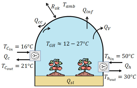
Figure 1.
Energy balance of a greenhouse with tomato crop.
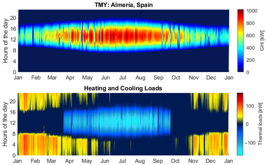
Figure 2.
Global horizontal irradiance of Almería, Spain, and calculated heating and cooling loads of the greenhouse with tomato crop.

Table 1.
Main characteristics of the greenhouse.
2.2. Individual Solar Photovoltaic and Solar Thermal Schemes for Cooling and Heating
For the case of solar electrically driven systems, the typical scheme for solar cooling with photovoltaic modules requires a battery set. However, due to the high cost of batteries and the repositioning period, the literature recommends integrating PV modules without batteries in refrigeration systems to improve economic performance and supply excess electricity for the internal consumption of the building. In this sense, the PV system comprises mono-crystalline silicon modules with an inverter without batteries to provide electricity to the AWCH with CTES, as shown in Figure 3a. The heating demand is supplied using a gas boiler. The thermal system consists of a flat plate collector field, a heat thermal energy storage (HTES), an auxiliary boiler (BL), a chiller unit for single-effect absorption (ABCH) of lithium bromide, and a cooling water tower (CWT), as shown in Figure 3b. The thermal systems cover the heating demand during winter and the heating for the ABCH in summer.
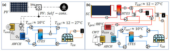
Figure 3.
Individual schemes: (a) solar photovoltaic with AWCH to supply renewable electricity and cooling; (b) solar thermal with ABCH to supply renewable heating and cooling.
2.3. Hybrid Solar Thermal and Photovoltaic System for Heating and Cooling Processes
The hybrid system combines the operation of the ST-ABCH system and the PV-AWCH system, as shown in Figure 4, of which the operation strategies are described in the next section. The application of the systems is evaluated considering the AWCH equipment as an auxiliary chiller. In that sense, the volume is lower than that of , and it is discharged in base on the maximum cooling load. Therefore, it has the fewest operating hours in the year. The excess of photovoltaic electricity () is used to supply electricity to the pumps and auxiliary components of the system. The schematic of the hybrid system with the coupled TRNSYS TYPES can be found in Figure A2.
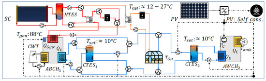
Figure 4.
Hybrid solar thermal and photovoltaic scheme with AWCH–ABCH to supply renewable electricity, heating and cooling.
2.4. Control for Discharge and Charge of the Thermal Energy to Heating and Cooling Processes
The control system for charging and discharging the refrigeration system is based on maintaining the CTES outlet temperature () equal to . The TRNSYS TYPE-1503 is used for the control, which simulates the operation of a thermostat. Equations (6) and (7) represent the maximum charging temperature () and the minimum charging temperature (). These reference temperatures are used for the activation of the signals () of the diverge (), the CTES pump and the ON/OFF of the chiller system ().
The control of the system is conditioned by the fulfillment of the cooling flow rate () and chiller flow rate (): ; and . The possible combinations of operation are shown in Table 2, in which there are four operation modes, and Figure 5 shows the reference temperatures and the control signals, where (A) shows the operation with a full discharge of the CTES, (B) shows the full charge of the CTES and the cooling supply to the process, (C) charges the CTES () and simultaneously covers the cooling demand (Pr). It should be noted that the auxiliary cooling system () works in conditions A, B and C, while in the main system (), condition (D) prioritizes the cooling demand coverage of the process, and depending on the chiller capacity, the flow is divided for the simultaneous loading of the CTES.
Table 2.
Control conditions for the charging and discharging of the cooling system.
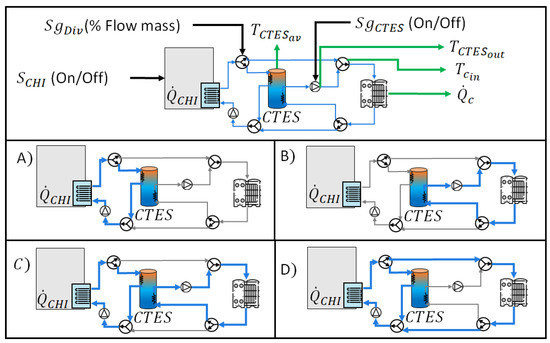
Figure 5.
Control conditions for the charging and discharging of the cooling system: (A) full discharge; (B) full charge; (C) partial charge of the CTES; (D) direct covering of cooling and partial charge of the CTES.
On the other hand, the HTES charge control is based on a hysteresis control that is activated based on the HTES outlet temperature and the maximum temperature reached by the solar field. At the same time, the PV system activates the when the state of charge (SOC) is less than 90%. The operation condition is based on adjusting the cooling capacity of the AWCH regarding photovoltaic production and is limited by the minimum flow mass according to the catalog [11,14].
3. Description of Solar Technologies and Chiller Simulations
The input data to evaluate PV and ST include the estimation of the solar radiation in the inclined plane (). In this research, the HDKR method is used to estimate , while the effective absorbed solar radiation (S) is solved assuming that the diffuse and ground-reflected radiation are isotropic, according to J. Duffie et al. [27]. The photovoltaic modules and solar collectors are positioned at an inclination equal to latitude and in a southerly direction.
3.1. Photovoltaic Modules and Inverter
The simulation of the PV field is carried out by applying the 5-parameter diode method [28] and the SANDIA temperature method [29] with MATLAB R2021a. For the joint simulation with the thermal solar field with TRNSYS, the resulting electrical power is loaded with Type-9. The De Soto model of the 5-parameter method [28] is as shown in Equation (8).
where is the light current, is the diode reverse saturation current, series resistance, is the diode ideality factor, k is the Boltzmann constant, is the number of PV cells in a series, is the cell temperature, is shunt resistance, I is current, and V is the voltage. is calculated using the SANDIA method [29], which is a function that requires as input variables a , and wind speed (), as shown in Equation (9).
where a and b are the coefficients defined depending on the module material type and assembly. is the temperature difference between the module and , while the inverter is solved using the SANDIA methodology of Equation (10), which estimates the transformation from direct current () to alternating current ().
where is the maximum power rating for the inverter at reference conditions, , , and are coefficients that are determined based on DC input voltage () and DC voltage level at which the AC power rating is achieved at reference operation conditions (). The methods for predicting the performance of the PV applied in MATLAB are validated using the PV field installed in CIESOL as a reference [30]. The evaluated system consists of an array of 14 modules connected in series with an inclination angle of 22 and an azimuthal angle of 21 east [31]. Figure 6 summarizes the combined method applied in MATLAB and shows the coefficient of determination (), root-mean-square error () and the relative difference ().
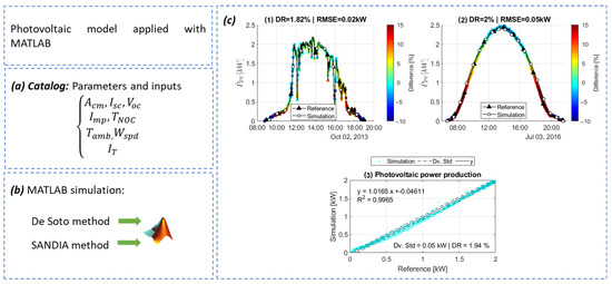
Figure 6.
Process scheme of the simulation of the PV with MATLAB. (a) Catalog input parameters; (b) data required to simulate the solar field; and (c) comparison of results obtained with CIESOL operation: (1) Variable day; (2) clear day and (3) standard deviation.
For this research, the library of NREL, accessed through the SAM software, is used to select the PV modules and inverters [32]. The selected PV module is the Seraphim-SEG-445 shown in Table 3, which contains the characteristics in standard conditions () as nominal efficiency (), maximum power (), short circuit current (), open circuit voltage (), maximum power current (), maximum power voltage () and nominal operating (), and the module area ().
Table 3.
Nominal operating parameters of the mono-c-SI photovoltaic module obtained from the SAM library.
3.2. Flat Plate Collectors (FPC)
Solar collectors are simulated with TRNSYS using the TYPE-1289, which is based on EN12975-2 Dynamic Efficiency Approach (ASHRAE IAMs). The method used to predict the performance of the flat plate collectors (FPC) with TRNSYS was validated by Z. Tian et al. [33]. The equations of the solar collector model are shown in Equation (11).
where is direct radiation on the inclined plane, () diffuse radiation on the inclined plane, and () reflect radiation on the inclined plane, is the collector temperature, is the incidence angles for the and components, and are the incidence angle modifiers for beam and diffuse radiation, respectively, () is the collector area and the useful heat, while () is the Zero-loss efficiency, () and () are the first and second order loss coefficients, respectively, () is the effective thermal capacity, and is the testing flow rate.
Figure 7a,b show the summary of the input parameters and the input data for the simulation of the FPC in TRNSYS. The validation was carried out with the CP1 Solaris collectors installed in CIESOL with a disposition of eight FPC connected in series with an inclination of 30 [34]. Figure 7c compares the measured outlet against the simulated data.
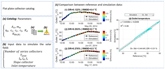
Figure 7.
Process scheme of the simulation of the FPC with TRNSYS. (a) Catalog input parameters; (b) data required for the simulation; (c) comparison of results obtained with CIESOL operation: (1) 5 May 2014; (2) 7 June 2014; (3) 17 May 2015 and (4) standard deviation.
Table 4 shows the coefficients of the HEATboost 35/10 collector that is used to develop the simulations with the greenhouse and the hybrid system proposed.
Table 4.
Parameters for predicting the behavior of the HEATboost 35/10 collector [33].
The auxiliary gas boiler is simulated using the TYPE-122, which consists of a simplified model to predict the auxiliary heating () based on the heat temperature set. The auxiliary energy input () is calculated with the boiler efficiency () and gas combustion efficiency ().
3.3. Air-Cooled Scroll Compressor Chiller (AWCH)
Polynomial regression is applied with MATLAB from the performance curves reported in the catalog data of the AWCH to characterize all the operating variables. The simulation of the AWCH is carried out with TRNSYS through TYPE-118 to resolve Equations (12)–(15), which are based on a polynomial regression from input data that contain the part load ratio (), current evaporator loads () which vary based on the , set temperature of the evaporator (), and the electrical consumption of the compressor ().
where is the external mass flow of the evaporator, is the specific heat capacity of the , is the evaporator leaving temperature, is the evaporator load, and is the heat rejection of the equipment. Figure 8a shows the procedure for the AWCH simulation. The equipment selected to simulate the PV-AWCH system is the YORK-YCAL0060EB with a nominal capacity of 169 kW, while the ST-PV hybrid system is used for the YORK-YCAL0024EB chiller with a nominal capacity of 76 kW [35]. Figure 8b,c show the behavior of the chiller for different ambient temperatures () and . The operating temperature is 10 C, and depending on the , the chiller reaches a capacity greater than 170 kW, which benefits the CTES.

Figure 8.
(a) Process scheme of simulation of the AWCH. COP and chiller capacity as a function of and ; (b) chiller: COP and nominal capacity of 76.6 kW; (c) chiller: COP and nominal capacity of 169.2 kW.
3.4. Method to Simulate the Performance of Single-Effect Absorption Chiller (SEABC Method)
The method is focused on obtaining the performance of the single-effect ABCH from a data catalog supplied by the manufacturer. However, the data are usually incomplete, requiring a system of equations to be solved for the ABCH in order to estimate the performance of the system under conditions not reported in the catalog, or failing that, the performance is obtained from experimental data. In this way, the is estimated under different operating conditions of , the cooling tower temperature (), and .
Due to the limitations on the data provided by the manufacturer, J. Martínez et al. [36] developed a method that is based on obtaining the total heat transfer coefficient value (), which is a coefficient of proportionality of the total UA values for the evaporator (), absorber (), generator (), desorption process heat exchanger (), and condenser (). However, the method is limited by being usable only with the YAZAKI chiller with 17 kW of cooling capacity. To resolve this gap, a general method is proposed to characterize the performance of a single-effect ABCH. From the data published by Martínez [36], it is possible to determine the ratio between capacity and total mean logarithmic temperature difference () to obtain , as shown in (16).
where is the instantaneous capacity of the chiller supplied by the catalog under nominal conditions, while to obtain the of each heat exchange, the coefficients of () reported by Martinez must be used, as shown in Equation (17).
where i are , , , and . Once the is obtained, it is possible to iterate the internal temperature of the evaporator and obtain the logarithmic temperature difference () and with Equations (18) and (19).
where () is the nominal external inlet temperature of the evaporator from the catalog, is the internal inlet temperature, and is the internal outlet temperature of the evaporator. It should be noted that, for this resolution, it is assumed that if the and have no variation, then remains fixed, and [37]. Figure 9 summarizes the temperature inputs and outputs for the case of the evaporator (EVA) of a single-effect ABCH.
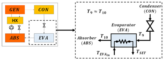
Figure 9.
Simplified diagram of input and output temperatures of the evaporator (EVA) for a single-effect ABCH.
Once has been estimated, the new evaporator capacity () is obtained by replacing with the fixed evaporator temperature (), while the generator temperature is corrected using an adaptation of the equations presented in [36], as shown in Equations (20)–(22).
where is obtained by replacing with . The previous correction allows a linear estimation that must be adjusted through polynomial regressions to determine the COP correction () of the chiller as a function of the variation of , and . The method to obtain the matrix of coefficients () that is used to determine is detailed in Appendix A. The polynomial equation () is solved using the data of reported in Table A1 and Equation (23).
where j is the number of coefficients of (), for simplicity, the vector is transformed to matrix , and Equation (24) is obtained.
where n is the number of coefficients of (). Then, it is possible to obtain with Equation (25).
The linear method is corrected by applying when the evaporator is higher than 8 C, using Equation (26).
Finally, the operation of the equipment, such as load design factor (), , and , is entered in a data script as a file (.txt). In TRNSYS, the system is simulated using TYPE-107 from the energy balance between the data script and Equations (27)–(31).
where is the cooling capacity, is the heat energy input, the subscript r indicates the reference instantaneous performance in nominal conditions, n shows the nominal performance of the chiller, is the design energy input fraction, is the nominal capacity fraction, is the heat rejected from the condenser, and is the electrical consumption of the equipment. The simulations are carried out with the YAZAKI SC-20, SC-30 and SC-50 chillers [38].
3.5. Energy Indicators of the Solar Cooling System
The simulations are compared based on energy indicators such as the , which is the ratio between the renewable energy contributed to the system and the energy required by the system. The equation that represents the for the hybrid system is based on SHC-Task 60 of the IEA Solar Heating and Cooling Programme [39] and is shown in Equation (32).
where is the useful power of the solar photovoltaic system, and P is the power consumption of the AWCH, ABCH, CWT and the pumps of the system. On the other hand, the overall conversion efficiency of the system () is calculated based on Equation (33).
where is the grid electricity consumption, is the sum of the solar field area of the PV and ST system, and are the cooling supply of systems 1 and 2, respectively. Finally, the fractional energy saving is calculated according to Eicher, S. et al. [40], which is the ratio between the fossil energy consumed by the renewable system and the reference energy consumed, as shown in Equation (34) [40].
where r is the electric and heating reference consumption without a solar system, based on the first scheme of the configurations presented in Figure 3a, and are the auxiliary energy to cover the electric and heat demand of the schemes PV-AWCH, ST-ABCH, HYB1 and HYB2.
4. Results and Discussion
4.1. Validation of SEABC Method
The method is validated using data from a YAZAKI SC-20 chiller with a nominal capacity of 70 kW supplied by the Solar Energy Research Center (CIESOL) in Almería, Spain. The SEABC methodology is applied with the data of the YAZAKI SC-20 chiller that contains performance curves of the single-effect ABCH with °C. Figure 10 shows the performance of the SC-20 chiller with a variation of , , and the evolution of . The maximum COP is 0.84 with °C, while the maximum capacity of the equipment is achieved with °C. Under certain theoretical conditions, the absorption cycle can reach values of COP up to 0.87 [37]. In addition, it can be observed that the capacity of the equipment and COP tend to grow with increasing .
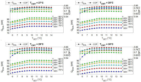
Figure 10.
Performance of YAZAKI SC-30 chiller applying the SEABC method as a function of the set temperature (), generator temperature () and cooling water tower temperature ().
CIESOL has used a centralized system that stores the data and supervises the operation of the ABCH since 2014. The data taken to validate the methodology correspond to 15 July 2015. Applying the SEABC method and comparing the measured temperatures with the simulation results, it was possible to observe that the differences tend to grow as the value increases above 12 C. Although the differences tend to be in ranges of less than 12%, the variation in the outlet temperature of the and can modify the behavior of the system.
Figure 11 shows the measured inlet and estimated outlet temperatures. It can be seen that the maximum difference is 10%, which is generated in periods in which C. In contrast, and maintain differences of less than 4 %, and the absolute difference is less than 5% for the estimated temperatures. Figure 12 shows a standard deviation (DV. Std) of less than 4 % with greater than 0.95. The best conditions for using the SEABC method are with under 12 C, due to differences of less than 7% being present in this case.
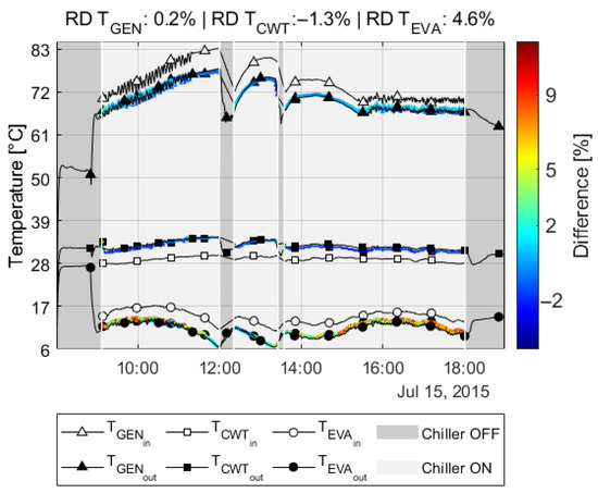
Figure 11.
Comparison between measured data vs simulation for 15 July 2015.
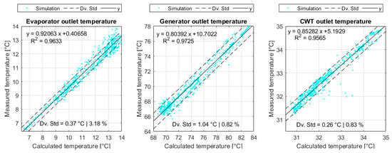
Figure 12.
Relative difference (DR) between estimated and measured values for each time step of ABCH YAZAKI SC-30.
4.2. Performance of the Absorption Chillers
The ABCH operating temperature should be chosen based on the performance of the equipment at °C. Figure 13 shows the COP and the cooling capacity with varying and for ABCHs of nominal capacity of 35 kW and 176 kW. The performance of the ABCH under nominal conditions with °C is shown in Figure A1. The heat map makes it possible to visualize the range of operation of the equipment to cover the cooling demand. In this sense, it is possible to improve the COP with °C, because it is advantageous to enhance the performance of the solar thermal system. However, the chiller capacity decreases by about 30% in such a case, while maintaining °C allows the COP to be kept close to 0.7. Based on the control system shown in Section 2.4, for periods of low cooling demand the maximum COP that it is possible to reach is fixed with a °C.
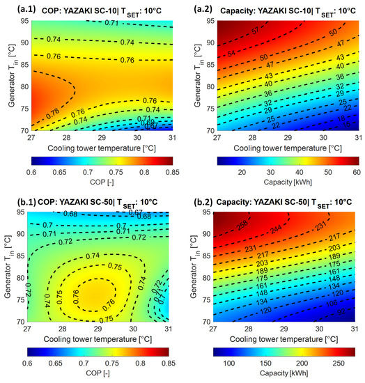
Figure 13.
Heat map: 1. Coefficient of performance and 2. capacity with a = 10 °C. Chiller YAZAKI: (a) SC-10 of 35 and (b) SC-50 of 176 .
4.3. Performance of the Hybrid Solar Cooling Systems
The section shows the results related to the PV-AWCH, ST-ABCH, HYB1, and HYB2 systems. Figure 14a shows the behavior of the AWCH of the individual PV system, the AWCH consumption electricity (), , and the COP for the day July 10th. Figure 14(b1) shows the total power production of the PV field (), the useful power consumed by the system (), and the power provided by the electric grid (). It can be observed that almost all of the is consumed by the PV-AWCH system. However, due to the charge control conditions and minimum of operation, there is a that tends to exceed the during the first hours of the morning and the last hours of the day. Figure 14(b2,b3) show the SOC of the system and the coverage of the cooling demand of the system with the main chiller (), respectively. The SOC of the CTES is close to a total discharge on July 9 and 10, due to the system prioritizing the CTES charge during radiation hours.
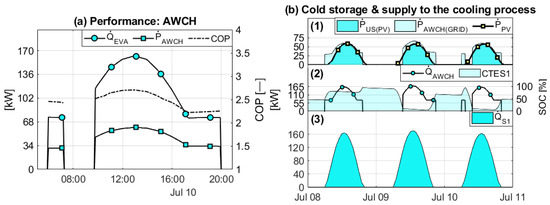
Figure 14.
Performance of the individual PV-AWCH system: (a) AWCH performance; (b.1) PV power generation; (b.2) CTES: SOC; and (b.3) the cooling demand covered.
Figure 15 shows the behavior of the individual ST-ABCH system. It is important to note that Figure 15a shows the performance of the ABCH with C, due to these results being recorded during the period of maximum system load. In addition, the ABCH increases its capacity by approximately 20% relative to its nominal capacity due to maintaining a C. However, the operating conditions make it necessary to maintain a heat demand of close to 300 kW, which means a heat demand from the generator that is greater than 40 % with reference to the heating demand. Figure 15b shows that, despite having a solar field area of 380 m, a contribution of close to 75% of the total demand is required during the first and last hours of the day. Figure 15c shows the SOC of the CTES in which the activation of the ABCH is appreciated once it reaches full discharge, maintaining coverage of of the cooling demand.
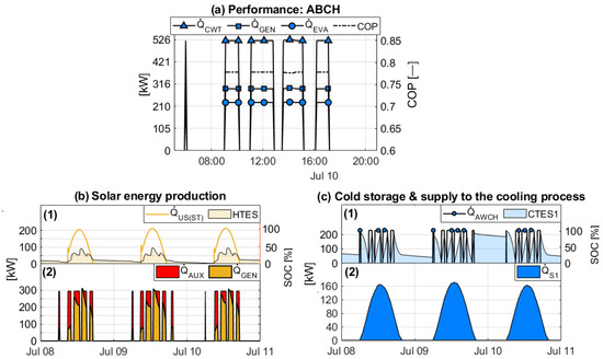
Figure 15.
The grid electricity consumptionsystem: (a) ABCH performance; (b.1) Useful heat and SOC of HTES; (b.2) solar thermal generation and auxiliary heat; (c.1) cooling supplied to the CTES and SOC and; (c.2) cooling demand covered.
Figure 16a shows the performance of the hybrid solar cooling system with the AWCH as the main chiller, with a nominal capacity () of 94 kW that can increase by with a of 10 C. Figure 16b shows the performance of the ABCH with a of 35 kW; in the same way, the performance of the ABCH can increase by 20% with respect to the nominal capacity. In contrast to the ABCH, the COP of the AWCH tends to increase over three if the is lower than 30 C. Figure 16(c1) shows that the is insufficient to cover the total power consumption of the system. On the other hand, Figure 16(c2) shows the and the SOC of the HTES that supply heat to . Figure 16(c3) shows that the decreases, and about 90% of heat is supplied, with the solar thermal system. Figure 16d presents the SOC of the CTES1 and CTES2 with respect to the performance of the ABCH and AWCH, respectively. In that sense, covers approximately 30% of the total cooling demand.
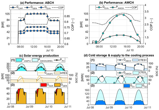
Figure 16.
Performance of the hybrid system with the AWCH as the main chiller (HYB1): (a) ABCH performance; (b) AWCH performance; (c.1) , and ; (c.2) SOC of HTES; (c.3) and ; (d.1) to CTES1 and SOC; (d.2) to CTES1 and SOC and; (d.3) cooling demand covered by S1 and S2.
On the other hand, Figure 17 presents the performance of the hybrid solar cooling system with an ABCH as the main chiller. The performance of the ABCH with a nominal capacity of 70 kW is shown in Figure 17. The energy efficiency of the HYB2 system shows an increase of around 100% of the heat flow to satisfy the demand of the . This allows to cover approximately of the cooling demand for the same time series. At the same time, 99% of the photovoltaic production is used to drive the AWCH, as shown in Figure 17c.
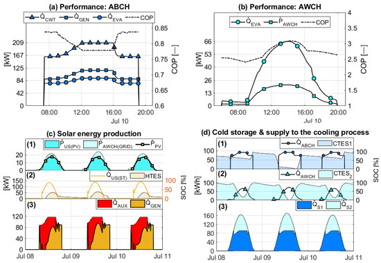
Figure 17.
Performance of the hybrid system with ABCH as the main chiller (HYB2): (a) ABCH performance; (b) AWCH performance; (c.1) , and ; (c.2) SOC of HTES; (c.3) and ; (d.1) to CTES1 and SOC; (d.2) to CTES1 and SOC and; (d.3) cooling demand covered by S1 and S2.
Figure 18 shows the monthly behavior of the individual PV-AWCH (a) and ST-ABCH (b) systems with solar field areas of 269 m and 244 m respectively. The annual () of the PV-AWCH system is 0.27, reaching a monthly () of 0.65 and 0.67 during July and August. During the winter and autumn months, the PV system covers the electrical demand of the heating system pumps. However, this is less than of the total energy consumption of the heating system. The advantage of the PV-AWCH lies in the high efficiency of the chiller, which is capable of reaching a COP higher than 2.5, which allows for attenuation of the low conversion efficiency of the PV modules. This means that the PV-AWCH system can achieve a system efficiency () of 0.85 and 0.77 in June and August, respectively.
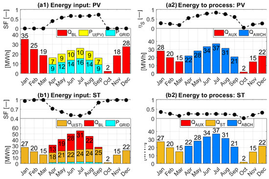
Figure 18.
Monthly system performance of the PV-AWCH (a) and ST-ABCH (b) systems: 1. and to the systems; 2. system efficiency and energy used for the heating and cooling processes.
On the other hand, the performance of the ST-ABCH system can achieve a of 0.72, due to having greater than 0.95 during the winter and autumn months. However, the maximum is 0.7 when the ABCH is on, decreasing to 0.49 during July. This is because the heat demand for the operation of the ABCH tends to be higher than the heating demand. In addition, it should be noted that the electrical consumption of the cooling system is around 5% of the total energy demand. Although the ST-ABCH system presents a high , the tends to be less than 0.3 during summer and less than 0.4 during winter, indicating an oversized solar field.
Figure 19 shows the hybrid system, which comprises a 244 m ST collector field and a 34 m PV field, totaling 278 m. The HYB1 (a) system with the AWCH as the main equipment achieves a of 0.86, whereas in July and August, it reaches of 0.72 and 0.74, respectively. The increases because the AWCH covers about 60% of the cooling demand, meaning a low heat demand requirement during the summer months. The energy reduction allows an of 0.6 to be achieved during the months with cooling demand, increasing the and of the ST-ABCH system, which has a similar solar field area.
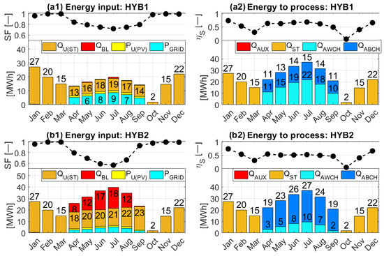
Figure 19.
Monthly system performance of the HYB1 (a) and HYB2 (b) systems: 1. and to the system; 2. system efficiency and energy used for the heating and cooling processes.
Meanwhile, the HYB2 (b) system increases heat demand because the ABCH covers 70% of the cooling demand. This results in a minimum of 0.6, due to the increased energy consumption of the boiler to supply the required heat to drive the ABCH. On the other hand, the efficiency increases to 0.5 and the consumption is reduced by around 40%, improving the indicators concerning the ST-ABCH reference system. However, the consumption of is increased by 99% with respect to the HYB1 configuration.
Regarding the annual results, Figure 20 shows the behavior of the PV-AWCH, ST-ABCH, HYB1 and HYB2 systems for the as a function of the solar field area, and the color bar shows the . The ST-ABCH reaches the maximum , with values close to 0.95, with a solar field larger than 700 m. However, the tends to be less than 0.2, due to the oversized area of the solar field with . Meanwhile, the PV-AWCH reaches a maximum of 0.35 because the system does not take advantage of the electrical production of the PV during winter, while the HYB1 reaches an higher than the reference systems from 120 m, reaching a maximum of 0.85 and an close to 0.4. On the other hand, the HYB2 shows improvements, with an area of 277 m compared to the ST-ABCH but with a lower than the HYB1.
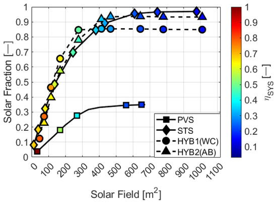
Figure 20.
and efficiency of the schemes: PV-AWCH, ST-ABCH, HYB1 and HYB2.
Figure 21 shows the behavior of the proposed schemes based on the area of the solar field, the area of the greenhouse, and the distribution of the . The red line marks the maximum recommended installation area, while the scatter plot with the color bar shows: the efficiency of conversion of the system (a), the fractional energy saved (), and the percentage of occupation of the FPC. The PV-AWCH configuration achieves a maximum of , due to only covering the demand of the electric systems (pumps and AWCH). However, the best result of the PV-AWCH configuration, considering the reference area as a limit of the size of the solar field, achieves an of with an area of 336 m and a 28%. On the other hand, the ST-ABCH configuration achieves an of 0.97 with an area close to 1000 m. Although the is close to 99%, the area of the solar field exceeds the reference area by 87%. The most favorable result of the ST-ABCH system is with a field of 434 m, capable of achieving and 84%. On the other hand, the HYB1 configuration achieves a maximum of and 84% with an area of 413 m. However, the best result of the HYB1 is placed with an area of 278 m, because it achieves 83% and . The HYB1 achieves similar results to those of the ST-ABCH system with an area of 380 m, but the HYB1 exceeds the by 11%, while the HYB2 achieves and 88% with an area of 414 m, which, relative to the ST-ABCH reference system, represents an increase of 3% and 4% in the and , respectively. On the other hand, the best result of the HYB2 concerning the reference area is achieved with an area of 278 m by reaching and 62%, which, in relation to the ST-ABCH system with a similar area, represents an improvement of 12% of and 40% of .
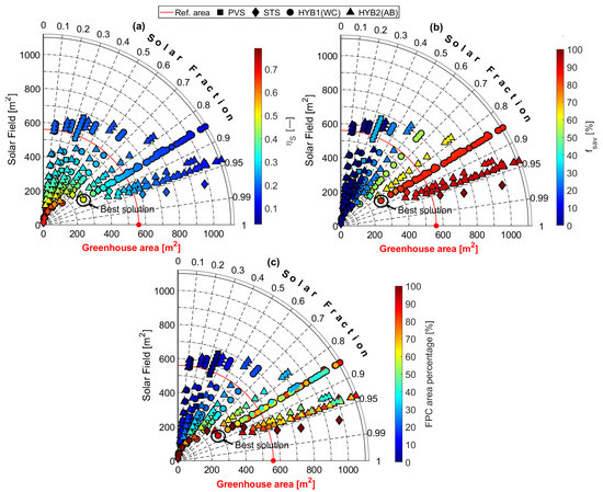
Figure 21.
Annual performance comparison among the individual photovoltaic system (PVS), individual solar thermal system (STS), hybrid (HYB) configuration 1 (WC) and 2 (AB). The colors of the scatter areas represent: (a) system efficiency (); (b) fractional energy saving (); and (c) FPC area percentage.
In light of the results obtained, it can be determined that the hybrid configuration with the best energy results is the second, which has an AWCH as the main equipment, achieving an of 0.85 and a fossil energy saving of 83% with a composition of 12% of PV modules, which means that the solar field occupies 50% of the reference area available.
5. Conclusions
This research focused on developing a methodology for modeling commercial single-effect ABCHs and their integration with hybrid solar refrigeration systems (ST-PV) applied to greenhouse air conditioning. The SEABC methodology was validated using MATLAB and data from the YAZAKI-SC20 chiller in operation at the Solar Energy Research Center (CIESOL). The simulation of the solar systems was carried out using TRNSYS, in which 228 cases of hybrid systems were simulated, varying the area ratio of the solar field and evaluating the differences between the use of an AWCH or an ABCH as the main chiller. The findings of this research can be summarized as follows:
- The SEABC method proposed in this research allows the operation of the ABCH to be replicated, taking as input parameters only six generator inlet temperature points and four cooling tower temperature points, and keeping the fixed.
- The precision of the SEABC method decreases with above 12 C. In contrast, the system’s performance with below 10 C allowed differences of less than 7% to be obtained, demonstrating that the method can predict the behavior of the ABCH with the nominal data and a low number of input temperature data.
- The evaluation of the , , and are necessary to determine the best hybrid configuration. The best results are achieved with the HYB1 configuration with an area of 278 m with a composition of 12% of photovoltaic modules, representing only a quarter of the greenhouse area.
- The increase in the energy efficiency of the HYB1 scheme is due to the AWCH covering most of the cooling demand. This makes it possible to limit the ST field to cover the heating demand and to use the ABCH as a renewable backup. This strategy minimizes the use of auxiliary energy in winter; however, as the capacity of the AWCH compared to the ABCH increases, the efficiency of the system tends to decrease.
Regarding future work, the main disadvantage of the photovoltaic field is that around 50% of the electricity production is lost during the winter months, so future work should evaluate the economic advantages of the hybrid system by adding a heat pump instead of selling the excess electricity produced, and the effects of the system’s performance in different climatic zones. In relation to the modeling method, it is advisable to compare the uncertainty of the SEABC method with other modeling methods based on data from different commercial chiller manufacturers. Finally, the investigation determined that the hybrid solar system focusing on the cooling process saves 83% of fossil energy with a PV-ST area close to a third of the total greenhouse area, which represents a potential contribution to reducing the carbon footprint of the agricultural sector.
Author Contributions
Conceptualization, A.V.-J. and R.E.; Methodology, A.V.-J. and R.E.; Formal Analysis, A.V.-J., J.F.R.-P., M.P.-G., J.M.C. and R.E.; Investigation, A.V.-J.; Resources, R.E.; Writing—Original Draft Preparation, A.V.-J. and J.F.R.-P.; Writing—Review and Editing, A.V.-J., J.F.R.-P., M.P.-G., J.M.C. and R.E.; Visualization, A.V.-J.; Supervision, R.E.; Funding acquisition M.P.-G., J.M.C. and R.E. All authors have read and agreed to the published version of the manuscript.
Funding
This research was partially funded by National Agency for Research and Development ANID BECAS/DOCTORADO NACIONAL 21200821 and 21200844. Also, this research received funding from projects ANID/FONDAP 1522A0006 “Solar Energy Research Center”-SERC-Chile.
Data Availability Statement
Not applicable.
Acknowledgments
Case study and validation data have been accessed thanks to the collaborative project MICROPROD-SOLAR of the Iberoamerican Program on Science and Technology for the Development (CYTED), supported by National Spanish Research Agency grant: PCI2019-103378. Andrés Villarruel-Jaramillo would like to acknowledge the funding from the National Agency for Research and Development ANID BECAS/DOCTORADO NACIONAL 21200821 and Josué F. Rosales-Pérez the funding from ANID BECAS/DOCTORADO NACIONAL 21200844. The authors wish to express their gratitude to the projects ANID/FONDAP 1522A0006 “Solar Energy Research Center”- SERC-Chile.
Conflicts of Interest
The authors declare no conflict of interest.
Abbreviations
The following abbreviations are used in this manuscript:
| Nomenclature: | |
| temperature difference between the module and | |
| flow mass | |
| heat flow rate | |
| efficiency | |
| zero-loss efficiency | |
| A | area |
| absorption chiller | |
| alternative current | |
| maximum AC power rating for the inverter at reference conditions | |
| air-cooled scroll compressor chiller | |
| specific heat capacity | |
| SEABC matrix of coefficients | |
| first order coefficient | |
| second order coefficient | |
| effective thermal capacity | |
| cooling capacity | |
| coefficient of performance | |
| cold thermal energy storage | |
| D | condition |
| direct current | |
| diverger | |
| standard deviation | |
| E | electricity |
| heat energy input | |
| excess of photovoltaic electricity | |
| design energy input fraction | |
| load design factor | |
| nominal capacity fraction | |
| fractional energy saving | |
| flat plate collector | |
| transpiration of sensible heat | |
| I | current | radiation |
| direct radiation on the inclined plane | |
| diffuse radiation on the inclined plane | |
| reflected radiation on the inclined plane | |
| radiation in the inclined plane | |
| k | Boltzmann constant |
| incidence angle modifiers | |
| number of PV cells in series | |
| diode ideality factor | |
| P | electricity power |
| part load ratio | |
| solar photovoltaic | |
| R | electric resistance |
| coefficient of determination | |
| S | effective absorbed solar radiation |
| general method to estimate the performance of simple effect absorption chiller | |
| solar fraction | |
| signal | |
| state of charge | |
| solar thermal | |
| standard conditions | |
| T | temperature |
| internal outlet temperature of the evaporator | |
| internal inlet temperature of the evaporator | |
| heat transfer coefficient value | |
| V | voltage |
| wind speed | |
| coefficients of UA | |
| total mean logarithmic temperature difference | |
| polynomial equation SEABC | |
| matrix reorganized | |
| Subscript: | |
| incidence angle | |
| a | annual |
| absorption | |
| alternating current | |
| ambient temperature | |
| auxiliary | |
| average | |
| boiler | |
| c | load thermals for cooling |
| gas combustion | |
| conduction–convection losses through the covert | |
| condenser | |
| chiller | |
| collector | |
| module | |
| maximum charging | |
| minimum charging | |
| compressor | |
| correction | |
| cooling water tower | |
| direct current | |
| e | electrical consumption |
| evaporator | |
| generator | |
| grid electricity consumption | |
| h | load thermals for heating |
| desorption process heat exchanger | |
| inlet | |
| infiltration losses with closed windows | |
| j | number of coefficients |
| L | light |
| logarithmic mean | |
| module | |
| maximum power | |
| monthly | |
| n | nominal |
| nominal operating cell temperature | |
| o | diode reverse saturation |
| open circuit voltage | |
| outlet | |
| p | number of coefficients of |
| r | reference |
| s | series resistance |
| main chiller of the cooling system | |
| auxiliary cooling system | |
| short circuit current | |
| shunt resistance | |
| radiation interchange through the greenhouse elements and the sky | |
| gain or loss of heat by the soil | |
| useful | |
| v | ventilation losses |
| w | testing |
Appendix A
Appendix A.1. SEABC Method
From the data of the chiller catalog, the of the equipment is extracted for a minimum of 20 points of and setting C. With the linear method, a vector is constructed that contains the COP for 29 C and °C. With Equation (A1), the coefficient matrix () is obtained.
Using MATLAB, a fourth-order polynomial regression is applied. The input data are and , in which the resulting coefficients must be ordered as shown in the coefficient matrix .
Then, a third-order polynomial regression is performed by inputting and , as shown in .
The process is repeated, varying C. Once all the matrices are obtained, it becomes possible from to to obtain the matrix of coefficients for each as shown ().
Applying a second order polynomial regression where and , it is possible to obtain a matrix of coefficients .
Table A1 shows the matrix correction coefficients applied to the YAZAKi SC-20 and SC-50 equipment.
Table A1.
Correction coefficients of the SEABC method applied to YAZAKI SC-20 and SC-50 chillers.
Table A1.
Correction coefficients of the SEABC method applied to YAZAKI SC-20 and SC-50 chillers.
| SC-20 | SC-50 | ||||
|---|---|---|---|---|---|
Figure A1 shows the performance of the YAZAKI SC-20 and SC-50 chiller under nominal conditions, based on the curves reported by the manufacturer.

Figure A1.
Heat map: 1. Coefficient of performance and 2. capacity with a = 7 °C. Chiller YAZAKI: (a) SC-20 of 70 and (b) SC-50 of 176 .

Figure A2.
Simulated hybrid system scheme with TRNSYS. (A) Complete system, (A.1) solar thermal subsystem and (A.2) cooling subsystem.
References
- United Nations; Framework Convention on Climate Change. Paris Agreement. 2015. Available online: https://unfccc.int/sites/default/files/english_paris_agreement.pdf (accessed on 25 May 2020).
- OECD; IEA. The Future of Cooling. 2018. Available online: https://iea.blob.core.windows.net/assets/0bb45525-277f-4c9c-8d0c-9c0cb5e7d525/The_Future_of_Cooling.pdf (accessed on 13 June 2020).
- Geraldi, M.S.; Ghisi, E. Building-level and stock-level in contrast: A literature review of the energy performance of buildings during the operational stage. Energy Build. 2020, 211, 109810. [Google Scholar] [CrossRef]
- Almasri, R.A.; Abu-Hamdeh, N.H.; Esmaeil, K.K.; Suyambazhahan, S. Thermal solar sorption cooling systems—A review of principle, technology, and applications. Alex. Eng. J. 2022, 61, 367–402. [Google Scholar] [CrossRef]
- Holka, M.; Kowalska, J.; Jakubowska, M. Reducing Carbon Footprint of Agriculture—Can Organic Farming Help to Mitigate Climate Change? Agriculture 2022, 12, 1383. [Google Scholar] [CrossRef]
- Carreño-Ortega, A.; Galdeano-Gómez, E.; Pérez-Mesa, J.C.; Galera-Quiles, M.D.C. Policy and Environmental Implications of Photovoltaic Systems in Farming in Southeast Spain: Can Greenhouses Reduce the Greenhouse Effect? Energies 2017, 10, 761. [Google Scholar] [CrossRef]
- Gil, J.D.; Ramos-Teodoro, J.; Romero-Ramos, J.A.; Escobar, R.; Cardemil, J.M.; Giagnocavo, C.; Pérez, M. Demand-Side Optimal Sizing of a Solar Energy–Biomass Hybrid System for Isolated Greenhouse Environments: Methodology and Application Example. Energies 2021, 14, 3724. [Google Scholar] [CrossRef]
- Cabrera, F.; Sánchez-Molina, J.; Zaragoza, G.; Pérez-García, M.; Rodríguez-Díaz, F. Chapter 8: Renewable energy technologies for greenhouses in semi-arid climates. In Sustainable Energy Developments, 13th ed.; Lovegrove, K., Stein, W., Eds.; CRC Press: Boca Raton, FL, USA, 2017; pp. 153–193. [Google Scholar] [CrossRef]
- Settino, J.; Sant, T.; Micallef, C.; Farrugia, M.; Spiteri Staines, C.; Licari, J.; Micallef, A. Overview of solar technologies for electricity, heating and cooling production. Renew. Sustain. Energy Rev. 2018, 90, 892–909. [Google Scholar] [CrossRef]
- NREL. Best Research-Cell Efficiency Chart. Available online: https://www.nrel.gov/pv/cell-efficiency.html (accessed on 6 April 2023).
- Eicker, U.; Pietruschka, D.; Schmitt, A.; Haag, M. Comparison of photovoltaic and solar thermal cooling systems for office buildings in different climates. Sol. Energy 2015, 118, 243–255. [Google Scholar] [CrossRef]
- Chen, Y.; Liu, Y.; Liu, J.; Luo, X.; Wang, D.; Wang, Y.; Liu, J. Design and adaptability of photovoltaic air conditioning system based on office buildings. Sol. Energy 2020, 202, 17–24. [Google Scholar] [CrossRef]
- Aguilar, F.; Crespí-Llorens, D.; Quiles, P. Techno-economic analysis of an air conditioning heat pump powered by photovoltaic panels and the grid. Sol. Energy 2019, 180, 169–179. [Google Scholar] [CrossRef]
- Aguilar, F.; Aledo, S.; Quiles, P. Experimental analysis of an air conditioner powered by photovoltaic energy and supported by the grid. Appl. Therm. Eng. 2017, 123, 486–497. [Google Scholar] [CrossRef]
- Luerssen, C.; Gandhi, O.; Reindl, T.; Sekhar, C.; Cheong, D. Levelised Cost of Storage (LCOS) for solar-PV-powered cooling in the tropics. Appl. Energy 2019, 242, 640–654. [Google Scholar] [CrossRef]
- Calise, F. Thermoeconomic analysis and optimization of high efficiency solar heating and cooling systems for different Italian school buildings and climates. Energy Build. 2010, 42, 992–1003. [Google Scholar] [CrossRef]
- Hirmiz, R.; Lightstone, M.; Cotton, J. Performance enhancement of solar absorption cooling systems using thermal energy storage with phase change materials. Appl. Energy 2018, 223, 11–29. [Google Scholar] [CrossRef]
- Prieto, J.; Ajnannadhif, R.; Fernández-del Olmo, P.; Coronas, A. Integration of a heating and cooling system driven by solar thermal energy and biomass for a greenhouse in Mediterranean climates. Appl. Therm. Eng. 2023, 221, 119928. [Google Scholar] [CrossRef]
- Villarruel-Jaramillo, A.; Pérez-García, M.; Cardemil, J.M.; Escobar, R.A. Review of Polygeneration Schemes with Solar Cooling Technologies and Potential Industrial Applications. Energies 2021, 14, 6450. [Google Scholar] [CrossRef]
- Rosales-Pérez, J.F.; Villarruel-Jaramillo, A.; Romero-Ramos, J.A.; Pérez-García, M.; Cardemil, J.M.; Escobar, R. Hybrid System of Photovoltaic and Solar Thermal Technologies for Industrial Process Heat. Energies 2023, 16, 2220. [Google Scholar] [CrossRef]
- Labus, J.; Bruno, J.C.; Coronas, A. Performance analysis of small capacity absorption chillers by using different modeling methods. Appl. Therm. Eng. 2013, 58, 305–313. [Google Scholar] [CrossRef]
- Puig-Arnavat, M.; López-Villada, J.; Bruno, J.C.; Coronas, A. Analysis and parameter identification for characteristic equations of single- and double-effect absorption chillers by means of multivariable regression. Int. J. Refrig. 2010, 33, 70–78. [Google Scholar] [CrossRef]
- Tawalbeh, M.; Aljaghoub, H.; Alami, A.H.; Olabi, A.G. Selection criteria of cooling technologies for sustainable greenhouses: A comprehensive review. Therm. Sci. Eng. Prog. 2023, 38, 101666. [Google Scholar] [CrossRef]
- Pérez Neira, D.; Soler Montiel, M.; Delgado Cabeza, M.; Reigada, A. Energy use and carbon footprint of the tomato production in heated multi-tunnel greenhouses in Almeria within an exporting agri-food system context. Sci. Total Environ. 2018, 628–629, 1627–1636. [Google Scholar] [CrossRef]
- ASABE. Heating, Ventilating and Cooling Greenhouses; ASAE EP 406.4; Technical Report; American Society of Agricultural and Biological Engineers: St. Joseph, MI, USA, 2003. [Google Scholar]
- Meteonorm V7.0.22.8. Available online: https://www.meteonorm.com/ (accessed on 20 January 2021).
- Duffie, J.A.; Beckman, W.A. Solar Engineering of Thermal Processes, 4th ed.; John Wiley and Sons, Ltd.: Madison, WI, USA, 2013. [Google Scholar] [CrossRef]
- De Soto, W.; Klein, S.; Beckman, W. Improvement and validation of a model for photovoltaic array performance. Sol. Energy 2006, 80, 78–88. [Google Scholar] [CrossRef]
- King, D.L.; Boyson, W.E.; Kratochvi, J.A. Photovoltaic Array Performance Model; Technical Report; SANDIA National Laboratories: Albuquerque, NM, USA, 2004. Available online: https://www.osti.gov/servlets/purl/919131 (accessed on 23 May 2022).
- Rosiek, S.; Batlles, F.J. Renewable energy solutions for building cooling, heating and power system installed in an institutional building: Case study in southern Spain. Renew. Sustain. Energy Rev. 2013, 26, 147–168. [Google Scholar] [CrossRef]
- Ramos-Teodoro, J. Energy Management Strategies in Production Environments with Support of Solar Energy. Ph.D. Thesis, Departamento de informática, Universidad de Almería, Almería, Spain, 2021. [Google Scholar]
- National Renewable Energy Laboratory; Golden, C. System Advisor Model Version 2020.11.29 (SAM 2020.11.29). Available online: https://sam.nrel.gov/photovoltaic/pv-sub-page-3.html (accessed on 3 June 2022).
- Tian, Z.; Perers, B.; Furbo, S.; Fan, J. Analysis and validation of a quasi-dynamic model for a solar collector field with flat plate collectors and parabolic trough collectors in series for district heating. Energy 2018, 142, 130–138. [Google Scholar] [CrossRef]
- Rosiek, S.; Batlles, F. Integration of the solar thermal energy in the construction: Analysis of the solar-assisted air-conditioning system installed in CIESOL building. Renew. Energy 2009, 34, 1423–1431. [Google Scholar] [CrossRef]
- Millennium®, Y. Model YCAL Style C Air-Cooled Scroll Chiller Engineering Guide. Available online: https://goo.su/fBxG (accessed on 7 July 2022).
- Martínez, J.C.; Martinez, P.; Bujedo, L.A. Development and experimental validation of a simulation model to reproduce the performance of a 17.6 kW LiBr–water absorption chiller. Renew. Energy 2016, 86, 473–482. [Google Scholar] [CrossRef]
- Manu, S.; Chandrashekar, T. A simulation study on performance evaluation of single-stage LiBr–H2O vapor absorption heat pump for chip cooling. Int. J. Sustain. Built Environ. 2016, 5, 370–386. [Google Scholar] [CrossRef]
- YAZAKI Energy Systems. Water-Fired Chiller/Chiller-Heater. Available online: http://jmp.sh/FacJtkG (accessed on 5 November 2021).
- Zenhäusern, D.; Gagliano, A.; Jonas, D.; Marco, G.; Hadorn, J.; Lämmle, M.; Herrando, M. SHC Task 60: Key Performance Indicators for PVT Systems. Technical Report, IEA SHC Task 60. 2020. Available online: https://www.iea-shc.org/Data/Sites/1/publications/IEA-SHC-Task60-D1-Key-Performance-Indicators.pdf (accessed on 2 February 2023).
- Eicher, S.; Bony, J. Definition of Main System Boundaries and Performance Figures for Reporting on SHP Systems. Technical Report, IEA-Solar Heating and Cooling Programme. 2013. Available online: http://www.iea-shc.org/data/sites/1/publications/T44A38_Rep_B1_SHP_Perf_definition%20approved.pdf (accessed on 23 April 2023).
Disclaimer/Publisher’s Note: The statements, opinions and data contained in all publications are solely those of the individual author(s) and contributor(s) and not of MDPI and/or the editor(s). MDPI and/or the editor(s) disclaim responsibility for any injury to people or property resulting from any ideas, methods, instructions or products referred to in the content. |
© 2023 by the authors. Licensee MDPI, Basel, Switzerland. This article is an open access article distributed under the terms and conditions of the Creative Commons Attribution (CC BY) license (https://creativecommons.org/licenses/by/4.0/).