Exergy Analysis and Off-Design Modeling of a Solar-Driven Supercritical CO₂ Recompression Brayton Cycle

Abstract

The latest generation of concentrated solar power (CSP) systems uses supercritical carbon dioxide (s-CO₂) as the working fluid in a high-performance recompression Brayton cycle (RcBC), whose off-design performance under different environmental conditions has yet to be fully explored. This study presents a model developed using the Engineering Equation Solver (EES) and System Advisor Model (SAM) to evaluate the operation of two solar-driven s-CO₂ RcBCs over a year, considering meteorological conditions in northern Chile. Under design conditions, the power plant outputs a net power of 25 $\mathrm{M}$$\mathrm{W}$ with a first-law efficiency of 48.3%. An exergy analysis reveals that the high-temperature recuperator contributes the most to the exergy destruction under nominal conditions. However, the yearly simulation shows that the gas cooler’s exergy destruction increases at high ambient temperatures, as does the turbine’s during off-design operation. The proposed cycle widens the operational range, offering a higher flexibility and synergistic turndown strategy by throttling the mass flow. The proposed cycle’s seasonal first-law efficiency of 39% outweighs the literature cycle’s 29%. When coupled to a thermal energy storage system, the proposed cycle’s capacity factor could reach 93.45%, compared to the value 76.45% reported for the cycle configuration taken from the literature.

1. Introduction

Renewable energy sources, including solar photovoltaic and wind, are increasing worldwide, comprising more than 10% of the global installed capacity for electricity generation in 2021 [1]. However, these sources cannot consistently deliver the required energy demand throughout the day due to their inherent variability. Incorporating energy storage technologies might allow higher penetration of renewables into the electrical grids, helping to overcome part of the challenges of energy transition [2]. Current and experimental CSP technologies can include thermal energy storage (TES) for increased dispatch flexibility and are, thus, an interesting option for dispatchable renewable power, especially in high solar radiation zones.

The installed capacity of concentrated solar power (CSP) technology has increased to more than $6.2$ $\mathrm{G}$$\mathrm{W}$, with Spain and the USA being the first adopters. However, an important number of projects are under development in the MENA region, South Africa, China, and Chile, among other countries [1]. Despite the increasing installed capacity of CSP technologies, the scientific community has been actively seeking technological improvements. One of the current research lines aims to implement new heat transfer fluids to operate TES systems at higher temperatures, increasing the power block’s conversion efficiency. The peak-load thermal-to-electric efficiency in the cycles commonly used in CSP systems is between 30% and 40% at turbine inlet temperatures lower than 600 °C. In contrast, conventional power plants can achieve efficiencies close to 58% using combined-cycle gas turbines [3]. Currently under development, the third generation of CSP considers a closed cycle using supercritical carbon dioxide (s-CO₂) as the working fluid, with the recompression Brayton cycle (RcBC) as the most prominent configuration [4].

Angelino [5] reported the first assessment of the performance of RcBCs using s-CO₂, finding thermal conversion efficiencies higher than 50% when driven by medium- to high-temperature sources. Since then, s-CO₂ has been studied as an interesting working/heat transfer fluid for different applications [6]. The potential of s-CO₂ RcBCs has sparked the interest of many, and they are under study for deployment in several applications, such as nuclear energy [7,8], solar energy systems [9,10], and marine propulsion [11].

Given the variability in the solar resource, RcBCs must achieve a high cycle efficiency under design conditions and maintain high thermal conversion efficiencies during off-design conditions. This translates into operation under a wide range of solar radiation and ambient temperatures for the power block.

Since TES-assisted CSP plants are commonly deployed in arid regions, water availability is another factor to consider for its implementation, which implies the implementation of dry cooling systems [12]. Therefore, the design and analysis of the system’s performance must consider its operation under variable environmental conditions.

Considering CSP plants’ large storage capacity, they commonly aim to maximize revenues by dispatching the electricity requested by the grid operator. Moreover, the flexibility of the dispatch is considered as one of the key features for addressing the issues that the growing capacities of solar photovoltaic plants and wind farms present for the grid, which, by nature, have a higher variability than CSP due to the latter’s thermal inertia and TES systems. Thus, the performance of RcBC should be analyzed in depth to assess its operation’s impact under variable conditions and the potential benefits of implementing these advanced cycles.

The technical potential shown by s-CO₂-motivated research is in the development of solar-driven RcBC power plants and improvement in the energy conversion efficiencies that commercial CSP plants present. Some works have been aimed at theoretically optimizing the cycle under strict constraints, e.g., ref. [13], while others endeavored to address the challenges posed by the particular characteristics of this working fluid, e.g., refs. [14,15], or investigated the economic trends in solar-driven s-CO₂ power plants coupled to a TES system, e.g., ref. [16]. Mature research started to include experimental studies in addition to theoretical ones. In this regard, the Sandia National Laboratories (SNL) test loop is one of the early experimental s-CO₂ power cycle test rigs [17].

Although conventional power plants operate at specific conditions for a given power output to mitigate disturbances, the variable nature of the solar resource induced the development of systems capable of storing surplus thermal energy to decouple power production from solar resource availability. The capacity of a power plant to manage the electricity dispatch according to the needs of the grid controller requires operation with high conversion efficiencies under off-design and not only at design conditions. Daylong operation in deserts with ample ambient temperature ranges implies that consistently maintaining the cycle’s low temperature throughout the day is economically unfeasible. Such conditions require specialized control systems that could isolate the power block from changes in ambient temperature or design power blocks that could handle the effects that a shifting cycle’s low temperature entails.

Dyreby [18] conducted a study addressing the need for a modeling approach capable of describing the performance of s-CO₂ cycles under off-design and part-load operational conditions by considering a turbomachinery model based on the performance maps reported by the Sandia National Laboratory (SNL9 test loop [19,20]). Although this work represents an important milestone in the off-design performance description of s-CO₂ RcBCs, the author considered several strong modeling assumptions, which are still considered in the current literature. Jahn [21] made further advances by applying empiric curves that describe the behavior of the turbine in off-design conditions. The study found that decreasing the turbine inlet temperature reduces the cycle’s net power output and proposed reducing the specific speed of the turbine–compressor shaft as a viable turndown strategy. Similar to Dyreby, Jahn did not consider a physical pressure drop model and used the constant conductance methodology to describe the off-design performance of the heat exchangers. Correa [22] reported an optimization procedure for the recompression fraction under off-design conditions subject to varying ambient temperature and heat supplied to maximize the cycle’s efficiency. This allowed assessment of the cycle’s performance under varying ambient temperatures and net power outputs. Recently, ref. [23] analyzed the dynamic behavior of a solar-driven CSP plant with an RcBC modeled using Dyreby’s methodology. The research aimed to optimize the TES system and solar field sizes to minimize the required auxiliary heating.

Variable energy supply, shifting ambient conditions, and demanding dispatch regimes configure a scenario where the assessment of the off-design operation is critical to the electricity market [24]. Therefore, a detailed description and modeling of the off-design operation of power cycles, especially the s-CO₂ RcBC, has gained larger attention in recent years. In that context, several models have emerged, varying in complexity and stiffness of their assumptions, as discussed in the previous paragraph. Nonetheless, there is still a gap for a holistic model that compiles the most detailed methodologies reported in the literature and revises those that rely on conditions unrepresentative of actual operation constraints; for instance, (i) the methodologies that disregard the pressure drop within heat exchangers led to alternate considerations, such as assuming a 1% pressure drop in all heat exchangers within the cycle [18], and (ii) modeling the non-linear relationship between the turbine and mass flow rate through a fixed-section nozzle based on the spouting velocity from an isentropic expansion. Thus, the probability of overlooking unknown phenomena when using simplified modeling methodologies is substantial and needs to be revised in detail.

The present study aims to further contribute to understanding the performance assessment of s-CO₂ RcBC by introducing a novel thermodynamic model validated against data reported in the literature. The model intends to assess the nominal performance of a power plant through first- and second-law efficiencies when considering the meteorological conditions of the Atacama desert, a high solar radiation zone with the potential for deploying solar-driven RcBCs. The modeling encompasses a detailed surge routine describing and predicting operational ranges and a detailed physics-based model for heat exchangers accounting for the pressure drops. In addition, the present article proposes an alternative configuration for RcBCs and a turndown strategy. Finally, the research describes the thermodynamic model utilized to assess the off-design operation of components and the RcBCs in a year operation through a quasi-stationary approach.

2. Methodology and Modeling

The following sections describe the modeling approach and the novel configuration proposed for exploiting the technical potential of the RcBC operating under variable conditions.

2.1. Cycle Design and Component Sizing

The cycle analyzed herein considers a capacity of 25 $\mathrm{MW}$, which is close to the limit for s-CO₂ radial turbine technology [21]. This net power output represents the cornerstone of the cycle design. Another constraint for the power cycle design is the cycle’s high-end temperature, i.e., the turbine inlet temperature (TIT). According to the literature, a reasonable (yet possibly ambitious) target is 650 °C. The cycle’s high-end and low-end pressures are 200 bar and 90 bar, respectively. A low cycle pressure of 90 bar allows the cycle to operate clearly above the critical pressure of CO₂ (i.e., $73.8$ bar). Although operating with a low low-end pressure increases the enthalpy drop through the turbine, there are related benefits in using a low cycle pressure higher than the critical pressure of CO₂. One may mitigate the adverse effects of operating near the critical point by increasing the low-end pressure. In this sense, two modeling decisions define the design low-end temperature $T_{low,design}$, i.e., (i) maintaining a fixed temperature pinch point within the cooler, and (ii) minimizing the product of power output and deviation from the design temperature. Hence, such modeling leads to the following equation:

$$\begin{array}{c}min\sum _i{M}_i{[(T_{db,i}+p)-T_{low,design}]}^2,\end{array}$$

(1)

where $M_i$ represents the demand multiplier in the dispatch matrix at the instance i of the TMY, $T_{db,i}$ the dry-bulb temperature at the instance i of the TMY, and p the pinch point of the cooler. Obtaining the low-end temperature from Equation (1) minimizes the differences between design and actual operation conditions weighted by the power output from the dispatch matrix and considers the weather data from Crucero in the Atacama Desert, northern Chile.

Figure 1 shows a schematic representation of an RcBC composed of a compressor, recompressor, low-temperature recuperator (LTR), high-temperature recuperator (HTR), primary heat exchanger (PHX), turbine, and cooler. The red and blue arrows indicate high- and low-pressure streams, while the green arrows refer to the molten salt stream.

One of the most important parameters for the RcBC design is the recompression fraction $\phi$. This was set to 0.3 based on the range of values reported in the literature [21,25]. The isentropic efficiencies of the turbomachinery were set as suggested by Jahn [21]. Compressor outlet pressure, recompressor inlet and outlet pressures, and turbine inlet and outlet pressures were chosen to achieve the high-end pressure at the turbine inlet and low-end pressure at the compressor inlet while considering the pressure drop through the cycle under design conditions. The recompressor inlet design temperature was set following the temperature resulting from the thermal conductance of the LTR and the HTR.

The turbomachinery was sized for maximal efficiency at the design point following the methodology described in Section 2.3 and Section 2.4. This translated into a flow parameter of $\varphi =0.297035$ for the compressors and a tip speed to spouting velocity ratio of $\nu =0.74376$ for the turbine. For the compressors, the $\varphi$ value, design inlet pressure and temperature, and design outlet pressure define the rotor diameter and design speed. The turbine diameter and design speed were also set to achieve the determined tip speed to spouting velocity ratio. The spouting speed depends on the design turbine inlet pressure and temperature and turbine outlet design pressure. Moreover, the heat transfer in the recuperators and pressure drop through the cycle affect the inlet pressures and temperatures and outlet pressures of the compressor, recompressor, and turbine. Therefore, an iterative process was implemented for properly sizing the previously mentioned components. Both the LTR and the HTR were modified, up-sized versions of those found in the SNL test loop [17]. Once the heat transfer and pressure drop were computed, the recuperator number of channels and length were varied until a cycle first-law efficiency near 50% was achieved. Due to the modeling constraints, the cooler and PHX were, therefore, determined from the power cycle energy balance. Likewise, no sizing routine was considered for the mixing chamber.

2.2. Literature vs. Proposed Cycle

A configuration of an s-CO₂ RcBC based on the cycle commonly reported in the literature was used to benchmark the performance of a novel configuration proposed. The literature cycle has two shafts, with the compressor and the turbine sharing the main one. Both shafts spin at variable speeds, with the recompressor shaft spinning to match the pressure at the high-pressure outlet of the LTR. This cycle is subject to the following constraints for off-design operation purposes:

• The cycle’s mass flow rate is equivalent to or lower than the design mass flow rate;
• The cycle’s high-end pressure is equivalent to or lower than the design high pressure;
• Pressure at any point in the cycle must be equivalent to or lower than the design cycle high pressure;
• Fixed TIT;
• Fixed recompression fraction.

The first three constraints allow evaluation of turndown control strategies that do not severely deteriorate the components of the power block, minimizing their lifespan reduction, considering an everyday off-design operation. Increasing the cycle’s mass flow rate and high pressure could increase its net power output. Still, the damage endured by equipment like the LTR, HTR, PHX, and cooler due to creep and fatigue cycling could result in long-term economic losses. The fourth constraint is due to the literature showing that the high-temperature control is a poor turndown strategy. The final constraint reduces the complexity of the problem by foregoing the optimization of the off-design operation. Throttling valves at the compressor and recompressor outlets ensure the cycle never surpasses the design’s high pressure.

The differences between the cycles described in the literature and the one proposed here are (i) the number of shafts, (ii) the cycle constraints, and (iii) the turndown strategy implemented. The proposed cycle considered three independent shafts. Regarding Figure 1, in the literature cycles, the compressor and the turbine spin at the same speed while the recompressor spins at a different speed; in the proposed cycle, all turbomachinery can spin at different speeds.

Regarding the control strategies, the literature cycle main shaft rotates at a speed depending on the mass flow rate required to achieve the desired power output. In contrast, the proposed cycle fixed the turbine’s spinning speed for all power output values. This reduced the flexibility of the proposed cycle, although it mitigated grid synchronization issues. By utilizing three independent shafts, the proposed cycle could reduce the rotational speed of both the compressor and recompressor shafts to modulate the high-end pressure. This allowed for a lower mass flow rate through the turbine, while the lower high-end pressure also decreased the turbine power output and the compressor power consumption. In contrast, the literature cycle cannot adjust the compressor speed independently from that of the turbine; thus, the pressure at the compressor outlet can surpass the design’s high-end pressure. The literature cycle considers two throttling valves to safeguard the integrity of the power block by reducing the compressor outlet pressure when it surpasses the design conditions.

The proposed cycle spun the compressor and the recompressor at the required speeds to provide the pressure the turbine needed to sustain a given mass flow rate. The literature cycle solves the compressor–turbine shaft speed necessary to achieve the desired mass flow rate whenever feasible. Then, considering the effect of the throttling valves, it solves the recompressor speed needed to match the pressures at the mixing chamber.

2.3. Turbine

The turbine model was based on Dyreby’s work [18], with a turbine isentropic efficiency defined as follows:

$$\begin{array}{c}{\eta }_{turbine}={\eta }_{turbine,design}(1.709\nu +1.55{\nu }^2-3.706{\nu }^3+1.297{\nu }^4),\end{array}$$

(2)

considering ${\eta }_{turbine,design}$ as the value at the design condition and $\nu =U/C_s$ tip speed U to spouting speed $C_s=\sqrt{2\Delta h}$ ratio—the latter is the speed that would be achieved if the fluid expanded isentropically within the turbine. Equation (2) evidences a maximum value at $\nu =0.74376$, as previously mentioned in Section 2.1.

The novel hybrid methodology applied extends such modeling, allowing the discarding of the constant nozzle area model and replacing it with one that considers the non-linear relationship between turbine operation parameters and mass flow rate. Ref. [21] models the non-linear relationship between turbine mass flow rate and operation parameters through the mass flow parameter ($MFP$) and the equivalent speed ($N_{eq}$):

$$\begin{array}{c}MFP=\dot{m}\frac{\sqrt{T_{in}}}{P_{in}},\end{array}$$

(3)

and

$$\begin{array}{c}{N}_{eq}=N\sqrt{\frac{T_{in}}{T_{design}}},\end{array}$$

(4)

where $T_{in}$ and $T_{design}$ are the temperatures at the turbine inlet and design conditions, respectively, $P_{in}$ is the pressure at the turbine inlet, and N is the shaft speed. MFP curves for radial turbines [26] were normalized and fitted through Stodola’s Ellipse Law Model [27] with two third-degree polynomials:

$$\frac{{\overline{MFP}}^2}{b{\left(\overline{N}\right)}^2}+\frac{a{\left(\overline{N}\right)}^2}{{\overline{\Pi }}^2}=1,$$

(5)

with $\overline{MFP}$ as the normalized mass flow parameter, $\overline{\Pi }$ as the normalized expansion ratio ($\Pi =P_{in}/P_{out}$), and $a\left(\overline{N}\right)$ and $b\left(\overline{N}\right)$ as third-degree polynomials that are functions of the normalized shaft speed:

$$\begin{array}{c}a\left(\overline{N}\right)=0.1364104{\overline{N}}^2+0.0166890\overline{N}+0.5190825,\end{array}$$

(6)

and

$$\begin{array}{c}b\left(\overline{N}\right)=-0.0264904{\overline{N}}^2+0.0852502\overline{N}+1.2918869.\end{array}$$

(7)

Hence, the proposed model given by Equation (5) is shaft-speed dependent, obtained by fitting to experimental data.

Considering that the TIT (i.e., the temperature at point 7 in Figure 1) is fixed in the present work, the functional form of the implemented model depends on the cycle constraints. The literature cycle operates with a variable turbine–compressor shaft speed. Considering Equations (3)–(5), the expression for the mass flow rate is as shown:

$$\begin{array}{c}\dot{m}=\frac{{\dot{m}}_{design}{P}_7}{P_{7,design}}b\left(\overline{N}\right){\left(1-{\left(\frac{a\left(\overline{N}\right)P_8{P}_{7,design}}{P_7{P}_{8,design}}\right)}^2\right)}^{\frac{1}{2}}.\end{array}$$

(8)

As indicated, the proposed cycle operates with a fixed turbine shaft speed; hence, the expression for the mass flow rate is as follows:

$$\dot{m}=\frac{{\dot{m}}_{design}{P}_7}{P_{7,design}}b\left(1\right){\left(1-{\left(\frac{a\left(1\right)P_8{P}_{7,design}}{P_7{P}_{8,design}}\right)}^2\right)}^{\frac{1}{2}}.$$

(9)

2.4. Compressors

Both the compressor and recompressor are modeled considering the curves obtained by Dyreby [18], based on the performance curves of the Barber–Nicholls compressor of the SNL test loop [17]. The same dimensionless methodology is used, with the compressor performance described as a function of the flow parameter:

$$\begin{array}{c}\varphi =\frac{\dot{m}}{\rho U{D}^2}\end{array}$$

(10)

and ideal head coefficient:

$$\begin{array}{c}\Psi =\frac{\Delta h}{U^2},\end{array}$$

(11)

where $\dot{m}$ is the mass flow rate, $\rho$ is the inlet density, U is the rotor tip speed, D is the rotor diameter, and $\Delta h$ is the isentropic specific enthalpy increase through the compressor. The shaft speed relates to the rotor tip speed as $U=\frac{DN}{2}$, with N as the shaft rotational speed. These coefficients and the expression for the isentropic efficiency are adjusted to account for changes in the shaft speed:

$$\begin{array}{c}{\varphi }^{*}=\varphi {\left(\frac{N}{N_{design}}\right)}^{\frac{1}{5}}\end{array}$$

(12)

$$\begin{array}{c}{\Psi }^{*}=\Psi {\left(\frac{N_{design}}{N}\right)}^{{\left(20{\varphi }^{*}\right)}^3}\end{array}$$

(13)

$$\begin{array}{c}{\eta }^{*}=\eta {\left(\frac{N_{design}}{N}\right)}^{{\left(20{\varphi }^{*}\right)}^5}\end{array}$$

(14)

where ${\varphi }^{*}$ is the modified flow coefficient, ${\Psi }^{*}$ is the modified ideal head coefficient, ${\eta }^{*}$ is the modified efficiency, and $N_{design}$ is the design shaft speed. ${\varphi }^{*}$, ${\Psi }^{*}$, and ${\eta }^{*}$ converse through polynomials:

$$\begin{array}{c}{\eta }^{*}=-0.7069+168.6{\varphi }^{*}-8089{\varphi }^{*2}+182725{\varphi }^{*3}-1638000{\varphi }^{*4}\end{array}$$

(15)

and

$$\begin{array}{c}{\Psi }^{*}=0.04049+54.7{\varphi }^{*}-2505{\varphi }^{*2}+53224{\varphi }^{*3}-498626{\varphi }^{*4}.\end{array}$$

(16)

Equation (15) evidences a maximum at the modified flow coefficient $\varphi$ = 0.297035, as previously mentioned in Section 2.1.

The predicted surge line is the basis for the implemented detailed surge prediction model. The predicted surge line was fitted twice under different independent and dependent variables. The first fit, $S_1$, mapped the predicted surge line as a function of normalized shaft speed to the flow parameter, i.e., $S_1\left(\overline{N}\right)\stackrel{}{\to }{\varphi }_{surge}$. For a given normalized shaft speed, the function returns the flow parameter at which surge is predicted to occur (${\varphi }_{surge}$). Thus, if the flow parameter is equal to or smaller than ${\varphi }_{surge}$, surge occurs. The second fit, $S_2$, mapped the predicted surge line as a function of the ideal head coefficient and flow parameter, i.e., $S_2(\Psi )\stackrel{}{\to }{\varphi }_{surge}$. Again, if the flow parameter is smaller than ${\varphi }_{surge}$ for a given ideal head coefficient, surge occurs. These functions are ${\Phi }_{surge}=0.0023100{\overline{N}}^2-0.0011521\overline{N}+0.0215676$ and ${\Phi }_{surge}=1.23234{\Psi }^2-1.10264\Psi +0.26802$, with $R^2=0.9982$ and $R^2=0.9958$, respectively. Both were used in conjunction to determine if and when the compressor or recompressor underwent surge. The criterion used was that both functions, $S_1$ and $S_2$, must predict the occurrence of surge for the model to treat it as such.

Similarly to the surge check functions, a simple check was implemented to assess if a compressor or recompressor was operating under a supersonic regime. The local Mach number was computed at turbomachinery outlets as $M=\left(\frac{DN}{2}\right)/c$, with c as the speed of sound. If M equaled or exceeded one, the compressor operated at a supersonic flow regime.

2.5. Compressors Partial Utilization (M out of N Systems)

The proposed model considers a system in which, instead of a single compressor and recompressor, there are three parallel smaller compressors and three parallel smaller recompressors. The sizes of these smaller devices depend on their proportional mass flow rates. This measure aims to introduce additional control variables that grant flexibility to the power block for off-design operation purposes.

When one or more compressors are turned off, the mass flow is divided equally between the remaining compressors, enabling the power block to work with lower mass flow rates without the compressors undergoing surge (at least, to a certain extent). A simplified modeling assumption was used in the numerical routine. The mass flow parameter was adjusted by the number of functioning compressors as ${\varphi }_{adjusted}=\varphi ·n/m$, with n being the number of compressors/recompressors and m the active number of compressors/recompressors. The number of active recompressors was independent of the number of active compressors; nonetheless, there was no point in adjusting one to account for a reduced mass flow rate without adjusting the other. Three configurations were defined, in which the number of active recompressors was chosen to increase the cycle’s operational range and first-law efficiency, given the number of active compressors.

Table 1. M out of N configurations.

Configuration	Literature		Proposed
	Comp.	Recomp.	Comp.	Recomp.
I	3	3	3	3
II	2	3	2	2
III	1	2	-	-

summarizes the number of operational compressors and recompressors for both the literature and proposed cycles under the different configurations.

2.6. Low- and High-Temperature Recuperators

Considering the high-pressure operation required by the s-CO₂, the LTR and HTR were considered as printed circuit heat exchangers (PCHE). These highly compact devices composed of diffusion-bonded microchannels can achieve high area-to-volume ratios and withstand large structural stress. The channels’ characteristic shape due to the etching process resembles a half ellipse. For channels of width $2a$ (i.e., the ellipse’s major axis) and depth b (i.e., the ellipse’s semi-minor axis), the following expressions describe their cross-sectional area, perimeter, and hydraulic diameter:

$$\begin{array}{c}A=\frac{\pi ab}{2},\end{array}$$

(17)

$$\begin{array}{c}P=2a+\frac{\pi }{2}\left(\frac{a+b}{2}\right),\mathrm{and}\end{array}$$

(18)

$$\begin{array}{c}{D}_h=\frac{8\pi ab}{8a+\pi (a+b)}.\end{array}$$

(19)

The cross-sectional area A arises from half of the area of an ellipse, the perimeter P is approximated as a sum of the major axis and a half circumference whose radius averages a and b, and the hydraulic diameter follows the standard definition $D_h=4A/P$.

For one hot and cold pair of channels of length L, the heat exchange area is given as follows:

$$\begin{array}{c}{A}_{channel,pair}=L·\left[2a+\frac{\pi }{2}\left(\frac{a+b}{2}\right)\right];\end{array}$$

(20)

hence, the total heat exchange area becomes the following:

$$\begin{array}{c}{A}_{LTR/HTR}=N_{channel,pairs}·L·\left[2a+\frac{\pi }{2}\left(\frac{a+b}{2}\right)\right],\end{array}$$

(21)

with $A_{LTR/HTR}$ as the heat exchange area of the recuperator and $N_{channel,pairs}$ the number of channel pairs.

The heat transfer in the recuperators considered Gnielinski’s correlation, while the pressure drops considered Petukhov’s correlation and Dostal’s expression for the inlet and outlet manifolds. The thermal resistance associated with the metal wall between streams in the PCHE was disregarded since its magnitude was negligible compared to the convective terms. Thus, the global heat transfer coefficient U depended only on the convection heat transfer coefficients for the hot and cold streams.

Both recuperators were discretized linearly into smaller recuperators along their length to account for the s-CO₂’s thermophysical property variations. Hence, the specific heat was approximately constant in each sub-heat exchanger, allowing for use of the $Q=UA\Delta T_{lm}$ model for counter-current heat exchangers. The HTR was discretized into four sub-heat exchangers, while the LTR was discretized into twenty sub-heat exchangers.

Each sub-heat exchanger’s pressure drop and heat transfer were assessed based on the local s-CO₂’s thermophysical properties. The flow speed v was assessed as a function of mass flow rate, channel cross-sectional area, number of channel pairs, and volume-specific mass:

$$\begin{array}{c}v=\frac{\dot{m}}{\rho ·N_{channel,pairs}·A},\end{array}$$

(22)

referring to one of the PCHE channels. This speed was then used to evaluate the Reynolds number $R{e}_{D_h}$, which in turn was used to assess both the friction form factor f through Petukhov’s correlation and the Nusselt number $Nu$ through Gnielinski’s correlation. With the Nusselt number, the convection heat transfer coefficient was obtained. These were then used to express the heat transfer and pressure drop equations coupled to the other sub-heat exchangers. This system of equations was then solved iteratively in the Engineering Equation Solver (EES)—a well-known general numerical equation-solving software that also includes a thermophysical properties database.

EES uses the Newton–Raphson numerical method, which tends to diverge when dealing with logarithmic mean temperature differences. The strategy adopted to mitigate such a characteristic was to solve the cycle using arithmetic temperature differences and then use the results as guess values for a second run of the EES program using logarithmic temperature differences. Since the recuperators were discretized, the temperature differences between one side and the other of the sub-heat exchangers became small enough to apply this approach.

2.7. PHX and Cooler

The primary heat exchanger (PHX) and cooler were modeled using a simplified approach. The outlet temperatures of both components were fixed, as were the pressure drops. The pressure drop in the PHX ($\Delta P_{PHX}$) was proportional to the pressure drop at the hot side of the HTR and the ratio between heat transfer in the HTR and the PHX. Likewise, the pressure drop in the cooler ($\Delta P_{Cooler}$) was proportional to the pressure drop at the cold side of the LTR and the ratio between heat transfer in the LTR and the cooler. These relations are summarized as follows:

$$\begin{array}{c}\Delta P_{PHX}=\Delta P_{HTR,hot}·\frac{Q_{PHX}}{Q_{HTR}},\end{array}$$

(23)

and

$$\begin{array}{c}\Delta P_{Cooler}=\Delta P_{LTR,cold}·\frac{Q_{Cooler}}{Q_{LTR}},\end{array}$$

(24)

with $\Delta P_{HTR,hot}$ and $\Delta P_{LTR,cold}$ as the pressure drops at the hot side of the HTR and the cold side of the LTR, respectively.

Such an approximation chooses the recuperator stream with the closest conditions to those in the PHX and cooler. The high-pressure HTR stream shares a similar pressure to the PHX, and the HTR outlet enters the PHX. The low-pressure stream of the LTR is the most akin to the cooler since it shares a similar pressure, and the LTR outlet proceeds to the cooler.

2.8. Cooler

The exit temperature from the cooler $T_1$ is variable. The working fluid always leaves the cooler at ambient temperature, with an added pinch point, defined as shown:

$$\begin{array}{c}{T}_1=T_{ambient}+p,\end{array}$$

(25)

in which $T_1$ is the low-end temperature at the cooler outlet, $T_{ambient}$ the ambient dry-bulb temperature, and p the pinch point. The pinch point was chosen at 15 $\mathrm{K}$ as a value representative of forced air cooling systems.

2.9. PHX

The s-CO₂’s PHX outlet temperature, i.e., $T_7$, was set to the design TIT of 650 °C. Hence, the mass flow rate of molten salts was such that the heat supplied equaled that absorbed by the s-CO₂:

$$\begin{array}{c}\dot{m}(h_7-h_6)={\dot{m}}_{salt}(h_{in,salt}-h_{out,salt}),\end{array}$$

(26)

with ${\dot{m}}_{salt}$ as the molten salt’s mass flow rate, and $h_{in,salt}$ and $h_{out,salt}$ as the molten salt inlet and outlet enthalpies, respectively. The temperatures at which the salt entered and exited the PHX were fixed at 700 °C and 550 °C, respectively. These temperatures enabled a TIT of 650 °C and ensured that the salt did not freeze. Moreover, because the molten salt enthalpies depended only on fixed temperatures and $T_7$ was also fixed, the molten salt mass flow rate ${\dot{m}}_{salt}$ was a function of s-CO₂’s mass flow $\dot{m}$, $P_7$, and $h_6$.

2.10. Exergy Accounting

The exergy accounting in the present study aims to identify the sources of exergy destruction, applying the exergy balance:

$$\begin{array}{c}{\Psi }_{in}={\Psi }_{out}+{\Psi }_{dest}\end{array}$$

(27)

in each component of the cycle, with ${\Psi }_{in}$ as the physical exergy that enters the component, ${\Psi }_{out}$ as the physical exergy outlet of the component, and ${\Psi }_{dest}$ as the physical exergy destroyed in the component. This expression takes different forms, depending on the cycle’s component. The expressions for ${\Psi }_{destroyed}$ for all components are below:

$$\begin{array}{c}\mathrm{Cooler}:{\Psi }_{dest,cooler}=\dot{m}(1-\phi )\left({\psi }_{10}-{\psi }_1\right)\end{array}$$

(28)

$$\begin{array}{c}\mathrm{Compressor}:{\Psi }_{dest,comp}={\dot{W}}_{comp}-\dot{m}(1-\phi )\left({\psi }_2-{\psi }_1\right)\end{array}$$

(29)

$$\begin{array}{c}\mathrm{Recompressor}:{\Psi }_{dest,recomp}={\dot{W}}_{recomp}-\dot{m}\phi \left({\psi }_3-{\psi }_{10}\right)\end{array}$$

(30)

$$\begin{array}{c}\mathrm{LTR}:{\Psi }_{dest,LTR}=\dot{m}\left((1-\phi )({\psi }_2-{\psi }_4)-({\psi }_9-{\psi }_{10})\right)\end{array}$$

(31)

$$\begin{array}{c}\mathrm{Mixing\; chamber}:{\Psi }_{dest,Mix}=\dot{m}\left((1-\phi ){\psi }_4+\phi {\psi }_3-{\psi }_5\right)\end{array}$$

(32)

$$\begin{array}{c}\mathrm{HTR}:{\Psi }_{dest,HTR}=\dot{m}\left(({\psi }_5-{\psi }_6)-({\psi }_8-{\psi }_9)\right)\end{array}$$

(33)

$$\begin{array}{c}\mathrm{Turbine}:{\Psi }_{dest,turb}=\dot{m}\left({\psi }_7-{\psi }_8\right)-{\dot{W}}_{turb}\end{array}$$

(34)

For molten salts, evaluating the physical exergy requires the assessment of enthalpy and entropy at a dead state, i.e., a thermodynamic condition where the salt is no longer molten but in a solid state. Mass-specific enthalpy and entropy for solid salts may be estimated through the following:

$$\begin{array}{c}h-h_0=c_{p,liquid}·(T-T_{fusion})+\Delta h_{fusion}+c_{p,solid}·(T_{fusion}-T_0)\end{array}$$

(35)

and

$$\begin{array}{c}s-s_0=c_{p,liquid}·ln\left(\frac{T}{T_{fusion}}\right)+\left(\frac{\Delta h_{fusion}}{T_{fusion}}\right)+c_{p,solid}·ln\left(\frac{T_{fusion}}{T_0}\right),\end{array}$$

(36)

where $c_{p,liquid}$ and $c_{p,solid}$ are the mass-specific heats of the molten and solid states, respectively, $T_{fusion}$ is the fusion temperature of the salt, and $\Delta h_{fusion}$ is the specific enthalpy of fusion. Considering the evaluation of the salt’s physical exergy was not the objective of this work; instead, it was the assessment of the exergy supplied by the salt. These expressions may be rewritten regarding enthalpy and entropy differences. Hence, the exergy destruction in the PHX becomes as follows:

$$\begin{array}{c}{\Psi }_{dest,PHX}={\dot{m}}_{salt}(\Delta h_{salt}-T_0·\Delta s_{salt})-\dot{m}({\psi }_7-{\psi }_6).\end{array}$$

(37)

2.11. Meteorological Conditions

The chosen simulation test site, Crucero, is an electrical substation in the Atacama Desert, far from any urban settlements. Its high direct solar irradiation is representative of the extensive arid plains of the Atacama Desert. Considering that electric utility companies generally seek to deploy power plants close to substations, solar radiation and environmental measurements from such a location are valuable for the potential assessment of solar energy systems.

The weather data used consider a typical meteorological year (TMY). For a specific geographical location, the TMY database reflects the long-term behavior of the meteorological conditions for every hour of the year. The TMY database reports direct normal irradiation (DNI), direct horizontal irradiation (DHI), dry-bulb temperature, relative humidity, pressure, wind speed, and wind direction. An important meteorological value is the direct normal irradiation design point, which is defined as the DNI value at 90% of the cumulative distribution function (disregarding night-time zero-values of DNI). That is, for the design point, the DNI is lower than the design point DNI at 90% of the sun-available time.

2.12. Dispatch Matrix and Annual Simulation

A dispatch matrix describes in a simplified way how the power plant output varies throughout the year on monthly and hourly bases. For instance, the dispatch matrix for a base-load power plant (e.g., nuclear power plant) is constant, denoting how the power output does not vary with time. On the other hand, a peaking power plant may have all values coinciding with times between 1 a.m. and 9 a.m. filled with zeros and values of 1 during the time windows that match peak electricity demand (e.g., 8 a.m. to 10 p.m.).

The demand-following dispatch matrix used in this work corresponds to one developed by Bravo [28]. It was composed of two dispatch curves, one for May through September and another for the remaining months.

An annual simulation using the meteorological data from Crucero and the dispatch curves mentioned above was carried out to gauge the efficiency of both the literature and the proposed cycles. A simplified model was used to couple the solar field to the power block whose data for the molten salt mass flow rate from the System Advisor Model (SAM) software was supplied to an energy storage EES code. That module provided the input heat that the power block required as a function of grid demand and ambient temperature. The heat supplied to the power block was expressed as a mass flow rate of molten salts, and the thermal energy storage was solved through the equivalent hot molten salt storage problem.

Because no specific dispatch strategy was used, the EES simulation sought to follow the dispatch matrix. However, if the plant’s outlet was insufficient to meet the required demand, the plant did not supply any power to the grid. SAM preset values for CSP power plants were used. A solar multiple of 4 was used to secure the heat supply for the power block, along with a TES system with 12 h of capacity. Due to the lack of information regarding the thermophysical properties of the mixture proposed by Mohan, solar salt’s properties were used as an approximation.

2.13. Seasonal Efficiencies

The cycle’s seasonal first- and second-law efficiencies quantify its performance, weighted by its net power output over the year. The seasonal first-law efficiency is expressed as follows:

$$\begin{array}{c}{\eta }_{season}=\frac{{\sum }_i{\eta }_i{\dot{W}}_{net,i}}{{\sum }_i{\dot{W}}_{net,i}},\end{array}$$

(38)

where ${\eta }_i$ and ${\dot{W}}_{net,i}$ are the cycle first-law efficiency and the net power output at hour i of the TMY, respectively. Likewise, the seasonal exergy efficiency is expressed as below:

$$\begin{array}{c}{\eta }_{ex,season}=\frac{{\sum }_i{\eta }_{ex,i}{\dot{W}}_{net,i}}{{\sum }_i{\dot{W}}_{net,i}},\end{array}$$

(39)

where ${\eta }_{ex,i}$ is the cycle second-law efficiency at the hour i of the TMY. As weighted averages, ${\eta }_{season}$ and ${\eta }_{ex,season}$ allow comparison of performances for a whole year of operation. These yearly indicators contrast with the instantaneous $eta$ and $et{a}_{ex}$, and are important when considering the cycles’ variable operation.

3. Results and Discussion

3.1. SNL Test Loop Benchmarking

The data reported in the literature regarding the operation of the SNL test loop was used to benchmark the results obtained from the numerical simulation implemented in EES and assess the cycle model’s capability to describe the operation of an s-CO₂ RcBC adequately. Only nominal operating conditions were considered for comparison due to the lack of off-design experimental data in the literature. The cycle information reported in refs. [17,20] was configured in the EES code to model the SNL test loop.

The results obtained from the EES code were used to determine performance parameters such as cycle efficiency, cycle input heat, cycle rejected heat, turbomachinery power consumption/generation, and heat load in and pressure drop through the recuperators. These parameters were then contrasted with those reported in ref. [20].

Table 2. Comparison against the SNL test loop.

				Scaled f
Variable	SNL	EES	Error [%]	SNL	EES	Error [%]
${\dot{Q}}_{out}$ [kW]	455	498.4	9.538	455	497	9.231
${\dot{Q}}_{in}$ [kW]	662	738.4	11.541	662	699	5.589
${\dot{Q}}_{LTR}$ [kW]	515	542.7	5.379	515	529.5	2.816
${\dot{Q}}_{HTR}$ [kW]	2202	2100	4.632	2202	2154	2.180
${\dot{W}}_{comp}$ [kW]	47.8	50.45	5.544	47.8	50.45	5.544
${\dot{W}}_{recomp}$ [kW]	85.1	79.59	6.475	85.1	79.65	6.404
${\dot{W}}_{turb}$ [kW]	331.1	370	11.749	331.1	332.1	0.302
${\dot{W}}_{net}$ [kW]	198.2	240	21.090	198.2	202	1.917
$\Delta P_{comp}$ [bar]	64.22	63.58	0.997	64.22	63.58	0.997
$\Delta P_{recomp}$ [bar]	62.89	61.96	1.479	62.89	62.18	1.129
$\Delta P_{turb}$ [bar]	52.95	58.18	9.877	52.95	52.96	0.019
$\Delta P_{LT{R}_C}$ [bar]	0.79	0.08972	88.643	0.79	0.79	0.000
$\Delta P_{LT{R}_H}$ [bar]	3.03	0.5643	81.376	3.03	3.03	0.000
$\Delta P_{HT{R}_C}$ [bar]	0.86	0.2516	70.744	0.86	0.86	0.000
$\Delta P_{HT{R}_H}$ [bar]	0.88	0.6989	20.580	0.88	0.88	0.000
$P{R}_{comp}$ [-]	1.84	1.827	0.707	1.84	1.827	0.707
$P{R}_{recomp}$ [-]	1.81	1.796	0.773	1.81	1.799	0.608
$P{R}_{turbine}$ [-]	1.64	1.736	6.144	1.64	1.636	0.030
${\eta }_{comp}$ [%]	67.3	66.36	1.397	67.3	66.36	1.397
${\eta }_{recomp}$ [%]	70.2	69.78	0.598	70.2	69.77	0.613
${\eta }_{turb}$ [%]	84.7	84.77	0.083	84.7	84.81	0.130
${\eta }_{cycle}$ [%]	29.9	32.5	8.552	29.9	28.9	3.472

summarizes the specific cycle parameters considered to validate the ability of the proposed model to describe the performance of an actual s-CO₂ cycle. For each variable in the first column of Table 2, the second column shows the magnitude reported in ref. [17] or ref. [20] (either directly available or determined using the available information). Moreover, the third column shows the results obtained from the EES model, and the fourth column the associated percentage error obtained from the EES routine concerning the data from SNL as $(100\times |SNL-EES|/SNL)$%.

In Table 2, $\Delta P_{comp}$, $\Delta P_{recomp}$, and $\Delta P_{turb}$ are the pressure rise/drop through the compressor, recompressor, and turbine, respectively. $\Delta P_{LT{R}_C}$, $\Delta P_{LT{R}_H}$, $\Delta P_{HT{R}_C}$, and $\Delta P_{HT{R}_H}$ are the pressure drops through the LTR cold, LTR hot, HTR cold, and HTR hot streams, respectively. Finally, $P{R}_{comp}$, $P{R}_{recomp}$, and $P{R}_{turb}$ are the pressure ratios of the compressor, recompressor, and turbine, respectively.

Some errors reported in the second, third, and fourth columns in Table 2 are significant. The higher values correspond to the pressure drops through the recuperators, the cycle net power output, turbine power output, and cycle first-law efficiency. Since the model underestimates the pressure drop through the test loop, it overestimates the pressure drop through the turbine. The first-law efficiency of a Brayton cycle depends on the turbine power output, which depends on the enthalpy drop through the turbine, and such a drop depends on the turbine working pressure difference. Therefore, one may argue that the error in cycle net power output, turbine power output, and cycle first-law efficiency all stem from underestimating pressure drop through the recuperators.

Considering the previous discussion, it was worth verifying the model’s ability to accurately account for pressure drop in the SNL test loop recuperators. Then, the friction factor f was scaled to match the data presented in ref. [17], removing the effects associated with the pressure drop within the recuperators on the numerical model. The fifth, sixth, and seventh columns of Table 2 (which are highlighted as Scaled f) show the updated results, indicating a major improvement, where the higher percentage errors were reduced to 1.92%, 0.30%, and 3.47% for net power output, turbine power output, and first-law efficiency, respectively.

Regarding the reduction in the errors obtained by adjusting the friction coefficient, the Petukhov [29], Blasius [30], and both empirical correlations of ref. [31] were implemented; however, the results showed that the errors increased. One possible explanation for such a behavior is that the relative surface roughness of the PCHEs plays an essential role in the pressure drop, and the tested correlations did not account for that. Although the surface roughness of PCHE might not be substantial ($\epsilon \sim$ 10${}^{-6}$ m [32]), their hydraulic diameter is small. In addition to that, the data provided by SNL correspond to experimental measurements, so they are subject to inherent uncertainties. The piping and its bends are not considered in the model, so they are possible sources of error. Moreover, there are experimental measurement uncertainties. In particular, the pressure drop through the hot side of the LTR stands out with a magnitude of $3.03$ bar, which could be due to the piping and instrumentation-related issues. Furthermore, Clementoni [17] states that leaks are an important problem of the SNL test loop, and mass losses throughout the test loop further hinder the model’s capability to describe the operation accurately.

3.2. Cycle Design

The power cycle analyzed herein considers a net power capacity of 25 $\mathrm{M}$$\mathrm{W}$ with a mass flow rate of s-CO₂ and molten salt of 255 $\mathrm{k}$$\mathrm{g}$/$\mathrm{s}$ and $224.6$ $\mathrm{k}$$\mathrm{g}$/$\mathrm{s}$, respectively, at the ambient design temperature of $20.8$ °C.

Table 3. Cycle pressure, temperature, enthalpy, and entropy under design conditions.

State	P [bar]	T [°C]	h [kJ/kg]	s [kJ/(kg K)]
1	90.000	35.80	−202.928	−1.407
2	200.277	58.89	−185.118	−1.401
3	200.254	134.25	−10.676	−0.9248
4	200.227	129.94	−18.509	−0.9441
5	200.227	131.22	−16.156	−0.9383
6	200.100	486.59	449.974	−0.09712
7	200.020	650.00	653.311	0.1453
8	90.789	544.29	530.044	0.1565
9	90.352	145.01	63.910	−0.6244
10	90.100	65.15	−52.716	−0.9362

summarizes the pressures, temperatures, enthalpies, and entropies for the s-CO₂ at each state of the cycle described in Figure 1.

The cycle’s design configuration ensures that the compressor and recompressor outlet streams are at equivalent pressure at the mixing chamber, $200.227$ bar. Such design pressure considers the pressure drops in the HTR and PHX, resulting in a turbine inlet pressure of $200.020$ bar.

Table 4. Cycle design dimensions.

Variable	Unit	Magnitude
D${}_{comp}$	[m]	0.2245
D${}_{recomp}$	[m]	0.2027
D${}_{turb}$	[m]	0.4637
N${}_{comp,design}$	[rev/min]	15,760
N${}_{recomp,design}$	[rev/min]	26,817
N${}_{turb,design}$	[rev/min]	15,760
A${}_{LTR}$	[m${}^2$]	3393
A${}_{HTR}$	[m${}^2$]	2962
N${}_{channelpairs,LTR}$	[-]	550,000
N${}_{channelpairs,HTR}$	[-]	600,000
L${}_{LTR}$	[m]	1.5
L${}_{HTR}$	[m]	1.2
a${}_{LTR}$	[mm]	0.8
b${}_{LTR}$	[mm]	0.8
a${}_{HTR}$	[mm]	0.8
b${}_{HTR}$	[mm]	0.8
D${}_{h,LTR}$	[mm]	0.9776
D${}_{h,HTR}$	[mm]	0.9776

and

Table 5. Cycle parameters under the design condition.

Variable	Unit	Magnitude
${\eta }_{comp,design}$	[-]	0.89
${\eta }_{recomp,design}$	[-]	0.89
${\eta }_{turb,design}$	[-]	0.93
$\Delta P_{comp}$	[bar]	110.3
$\Delta P_{recomp}$	[bar]	110.2
$\Delta P_{turb}$	[bar]	109.2
$\Delta P_{LT{R}_C}$	[bar]	0.05013
$\Delta P_{LT{R}_H}$	[bar]	0.2523
$\Delta P_{HT{R}_C}$	[bar]	0.1265
$\Delta P_{HT{R}_H}$	[bar]	0.4366
$\Delta P_{Cooler}$	[bar]	0.1
$\Delta P_{PHX}$	[bar]	0.08
P${}_{high}$	[bar]	200
P${}_{low}$	[bar]	90
T${}_{high}$	[°C]	650
T${}_{low}$	[°C]	35.8
${\dot{Q}}_{LTR}$	[MW]	29.740
${\dot{Q}}_{HTR}$	[MW]	118.864
${\dot{Q}}_{in}$	[MW]	51.851
${\dot{Q}}_{out}$	[MW]	26.813
${\dot{W}}_{comp}$	[MW]	3.179
${\dot{W}}_{recomp}$	[MW]	3.216
${\dot{W}}_{turb}$	[MW]	31.433
$\varphi$	[-]	0.3
$\dot{m}$	[kg/s]	255
${\dot{m}}_{salt}$	[kg/s]	224.6
${\dot{W}}_{net}$	[MW]	25
${\eta }_{cycle}$	[-]	0.483

list the main dimensions and parameters considered for the power cycle.

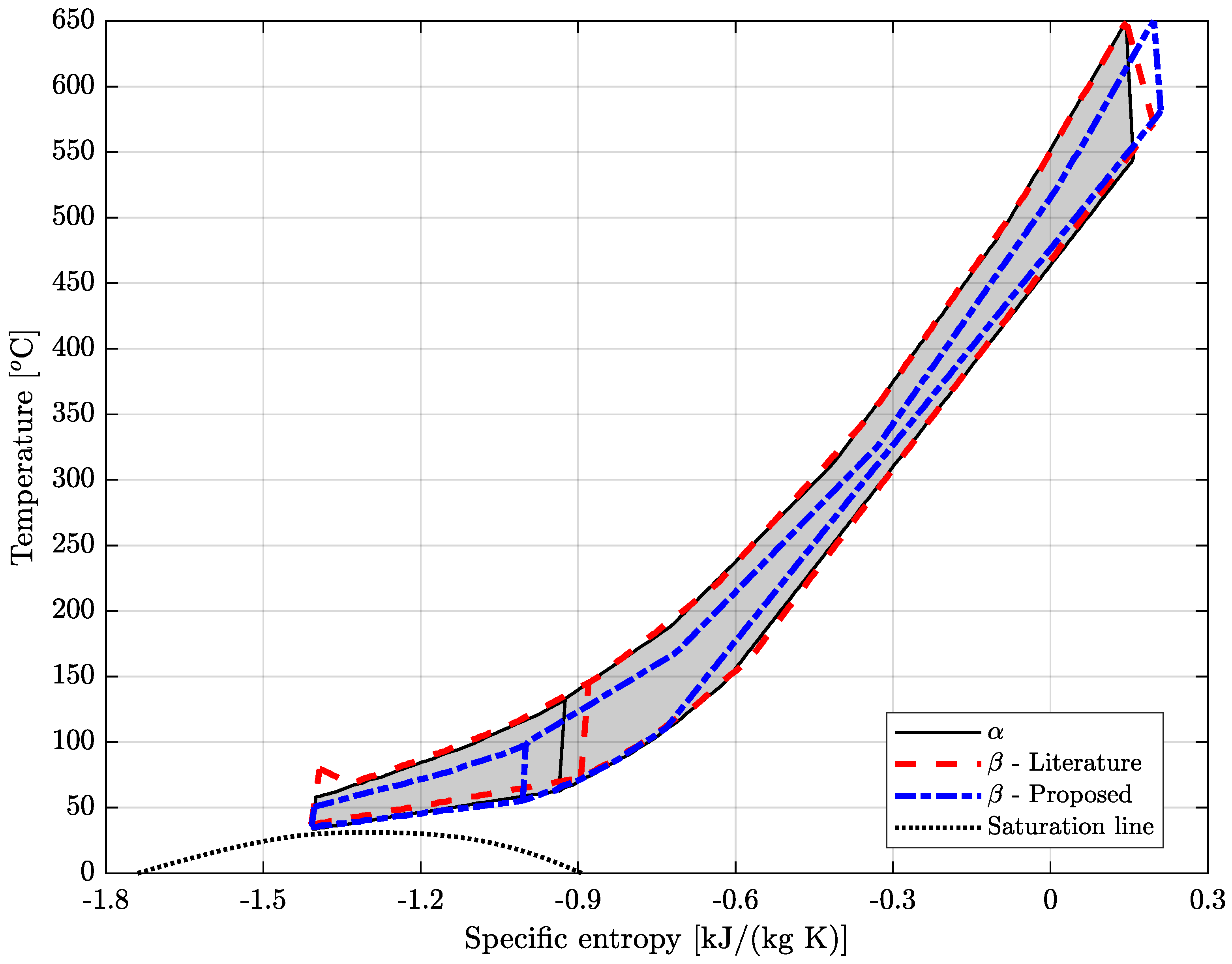
3.3. Literature Cycle

Figure 2 presents the operational ranges obtained for the literature cycle under different M out of N operation regimes as shaded regions. The x-coordinate corresponds to ambient temperature, and the y-coordinate corresponds to the percentage of the plant’s design net power output, i.e., 25 $\mathrm{M}$$\mathrm{W}$.

The gray region in Figure 2, delimited by the continuous black lines, indicates that the operational range of the literature cycle is highly restricted. On the domain of interest, the literature cycle can only operate on a thin crescent determined by three curves. The curve that describes the bottom-left end of the operational domain corresponds to the compressors undergoing surge. Since the power output is modulated through a decrease in the working fluid mass flow rate, the compressors rapidly undergo surge due to the proximity of the design operational condition to the surge line. As the ambient temperature increases beyond the design point, the s-CO₂’s mass-specific volume increases, decreasing the mass flow rate required to turn down the power output. This is partially offset by the increase in the mass-specific volumetric flow, delaying the onset of surge in the compressors and extending the operational range downwards. On the contrary, as the ambient temperature drops, decreasing the volumetric flow also causes the compressor to undergo surge. The literature cycle cannot operate at ambient temperatures below 7 °C, even at the design mass flow rate (i.e., 255 $\mathrm{k}$$\mathrm{g}$/$\mathrm{s}$).

Two different lines clearly define the right-hand side of the mid and dark-blue operational domain. The bottom one, at an ambient temperature of 28 °C, corresponds to the limit at which flow in the compressors becomes supersonic. The turbine pressure difference must be higher at higher ambient temperatures to achieve the same mass flow rate. Such a high-pressure difference can be achieved, to a certain extent, by increasing the rotational speed of the compressors; however, it is limited, since the compressor rotor tip speed eventually reaches Mach 1. Hence, the final edge of the mid- and dark-blue operational domain, i.e., the top-right end, corresponds to a new phenomenon not related to choking or supersonic flow. Specifically, operating at the top right corner requires the turbine to rotate slower while the compressor must spin faster. Since these components share a shaft in the literature cycle, a blockage occurs due to their mechanical integrity. Henceforth, this phenomenon represents a shaft blockage.

When the literature cycle operates with two of its three compressors and three of the three recompressors, the operational domain widens and shifts towards the lower left-hand corner, i.e., the blue region of Figure 2 delimited by the dashed blue lines. The surge limitation persists, although the mass flow rate is redistributed between fewer compressors, which delays its onset and enables the cycle to operate at an ambient temperature of 0 °C. The right-hand-side edge of the operational domain corresponds to the previously mentioned shaft blockage phenomenon. The increased mass flow rate the compressors perceive when one of them is turned off decreases the pressure rise through them. Reducing the volumetric flow is required due to a decrease in the ambient temperature to provide the pressure difference required by the turbine. Therefore, the shaft blockage curve shifts to the left compared to the previous region.

The red region under the dotted red line in Figure 2 corresponds to the one-out-of-three-compressors scenario. In this scenario, the surge limitation persists; however, since the domain of interest does not encompass power outputs smaller than 9 $\mathrm{M}$$\mathrm{W}$, it disappears as the domain edge for the last scenario. The upper-right curve corresponds to the shaft blockage phenomenon analogously to the one described for the previous configuration.

Overall, superposing the three operational ranges shows an extended operational range substantially larger than that available to the literature cycle if the M out of N strategy was not implemented. Regardless, the literature cycle cannot operate at ambient temperatures above 28 °C. There is a slight overlap between the third and second configurations; thus, the operational domain is continuous. However, the need to change between operating regimes on such a narrow band is challenging. Finally, this analysis corroborates the limits of the operational range for the literature cycle.

Combining the three previous configurations, the coupled first-law efficiency of the literature cycle over its operational range shows a maximum of 48.3% at design conditions and a minimum of 28% at off-design conditions. The first-law efficiency decreases slowly as ambient temperature decreases and faster as power output reduces, i.e., lower mass flow rate. Moreover, some discontinuities exist between the configurations’ responses, implying that a continuous change in the power block’s net power output would require a discrete change in the heat supplied to the cycle when changing between configurations. Also, when crossing the border between configurations at a constant mass flow rate, there is a discontinuity in the net power output, which brings out the importance of control ramifications.

3.4. Proposed Cycle

Figure 3 presents the operational range of the proposed cycle under different operation regimes (M out of N). The gray region delimited by the continuous black lines represents the wide domain where the proposed cycle can operate with three of its compressors on. The edge of the operational range is comprised of three curves: one at the bottom left-hand side and the other two at the right-hand end of the operational range. Comparing its operational range to the literature cycle evidences higher flexibility. As with Figure 2, the bottom left-hand edge corresponds to the compressors undergoing surge. Since neither the compressor nor the recompressor shares a shaft with the turbine, they can adjust their shaft speeds individually and delay the onset of surge. Furthermore, the right-hand side has a short curve at the top, where the limiting factor is the mass flow rate. At the maximum mass flow rate (255 $\mathrm{k}$$\mathrm{g}$/$\mathrm{s}$), the cycle’s net power output decreases as the ambient temperature increases. At higher ambient temperatures, the operational range is delimited by the onset of supersonic flow. As for the literature cycle, the pressure differential required to sustain a specific mass flow rate increases with higher ambient temperatures. The larger speeds eventually make the compressors enter a supersonic flow regime.

The blue region under the dashed blue line in Figure 3 describes a similar condition to the one observed in Figure 2. The cycle’s operational range exceeds the domain of interest on the left-hand side of the graph when operating with two out of its three compressors. The edge of the operational domain at the right-hand side is composed of a short curve associated with the maximum mass flow rate constraint and a long curve representing the limit of supersonic flow. Analogously to Figure 2, with one of the compressors off, the other two receive a larger mass flow rate, reducing the pressure rise, and the compressor must spin faster to sustain the required mass flow rate through the turbine, leading to the supersonic flow. Therefore, the right-hand side limit of the operational range shifts to the left-hand side. The extensive range of the proposed cycle under the two-out-of-three configuration makes analyzing the one-out-of-three configuration unnecessary.

The coupled operational range for the proposed cycle, shown in Figure 3 and obtained by superposing both operational ranges, indicates that the cycle can deliver power at an ambient temperature of 37 °C, albeit at little more than 50% of the design net power output. Moreover, it is observed that the overlap between the operational regions is significant (i.e., the dark-blue region).

Concerning the first-law efficiency, the minimum value observed for the proposed cycle is above 40%, exceeding the performance of the literature cycle (28%). Moreover, unlike the discontinuities found for the coupled efficiency of the literature cycle, the transition between configurations in the proposed cycle is smooth, eliminating the aforementioned control complexity. Also, the first-law efficiency varies strongly with net power output, but it varies more slowly when the ambient temperature is close to 27 °C. As for the literature cycle, the first-law efficiency varies less with respect to the ambient temperature as it decreases.

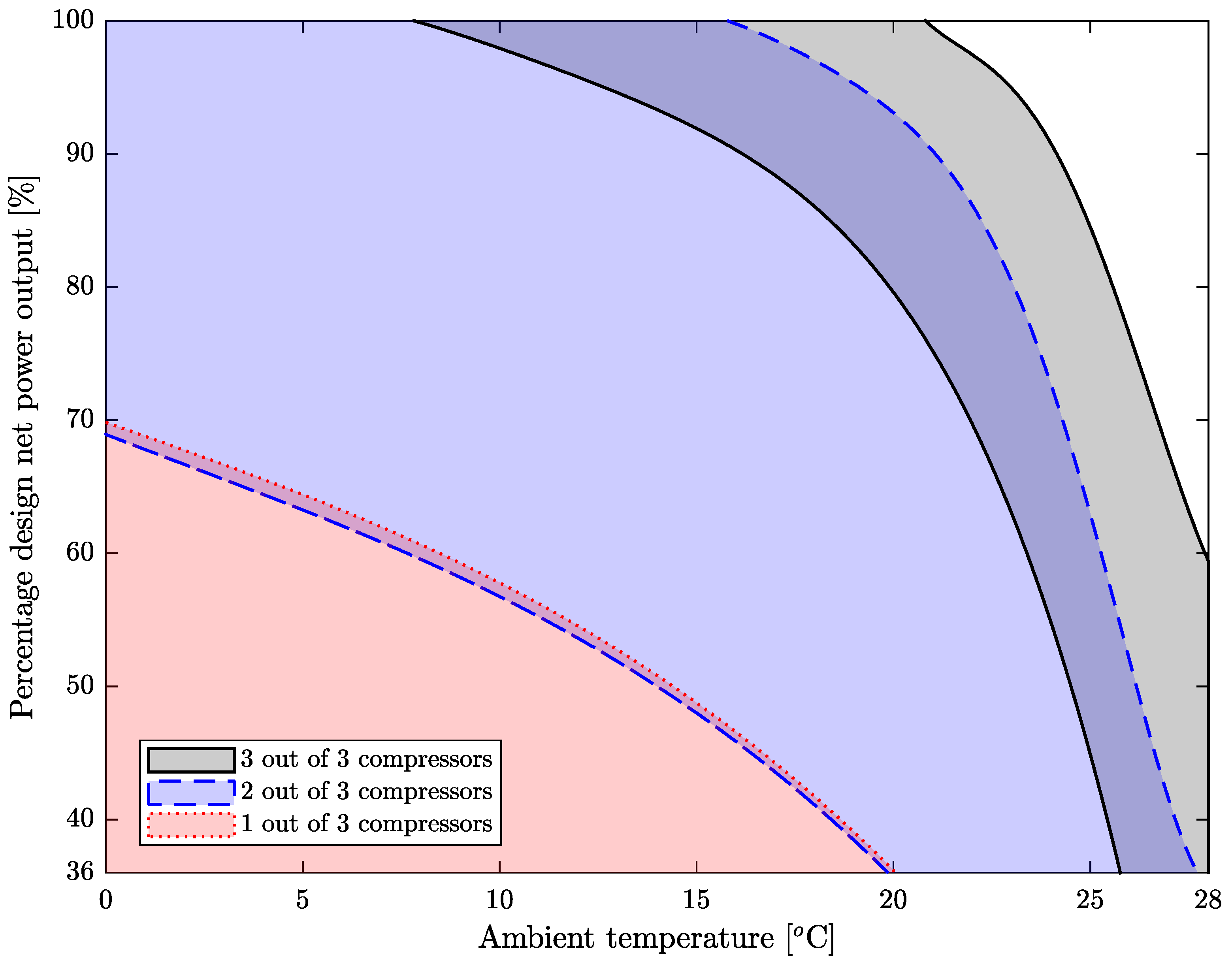
3.5. Influence of the Ambient Temperature and Net Power Output on the Cycle’s Performance

Aiming to examine the performance of both the literature and the proposed cycles, Figure 4 shows their combined operational range at specific key points, indicated using Greek letters. Additionally, the T–s diagrams are plotted along with the CO₂’s saturation curve to allow visualization of the changes in the cycle performance due to variations in the ambient temperature and cycle’s net power output.

Figure 5 presents the T–s diagrams of the cycle under nominal operational, i.e., at point $\alpha$— where the literature and the proposed cycles are identical —with the continuous black line (and shaded area), and the literature and proposed cycles at point $\beta$ with the dashed red and dash-dotted blue lines, respectively. At point $\alpha$, the cycle’s lowest temperature is close to the critical point, but, since the LTR outlet (i.e., where the flow splits) is further to the right side, the influence of the critical region is not significant. Due to the discretization considered by the model in the recuperators, the HTR part of the diagram does not have as many nodes as the LTR, which explains the sharp straight segments observed in that section of the diagram. Likewise, after the flow splits, the state corresponding to the cooler outlet causes a straight line at the bottom-left of the graph.

With an ambient temperature equivalent to the design ambient temperature and a power output of 9 $\mathrm{M}$$\mathrm{W}$, the literature cycle at point $\beta$ undergoes three important changes, as observed in the T–s diagram. The slope of the expansion curve shows an appreciable reduction in the turbine’s efficiency. The flow splitting occurs at a slightly higher temperature, shifting it to the right side along the specific entropy axis. Due to the reduced mass flow rate and the inability of the compressor to adjust its speed independently of the turbine speed, the compressor outlet pressure increases and the throttling valve reduces it, resulting in a bump at the compressor outlet.

On the other hand, the proposed cycle at $\beta$ shows three changes in its T–s diagram. The first change is a decrease in temperature at the splitting point, shifting it towards the left-hand side. The second change is the decrease in the cycle’s high-end pressure, as seen by the down-shifting of the top curve in the diagram. This is explained by the control strategy implemented, which considers the three-shaft layout to modulate net power output, decreasing its high-end pressure. Hence, unlike the literature cycle, there is no need for throttling valves after either the compressors or the recompressors. This reduction in the cycle’s high-end pressure, in turn, reduces the differential pressure through the turbine, reducing the enthalpy drop and, thus, the turbine power output. The third and final change is a decrease in temperature difference between streams in the HTR, explained by the discretization implemented.

Similar to Figure 5, Figure 6 presents the T–s diagrams of the cycles at point $\alpha$ with the continuous black line (and shaded area), the literature cycle at point $\gamma$ with the dashed red, and the proposed cycle at point $\delta$ with the dash-dotted blue line. At point $\gamma$, the cycle operates at an ambient temperature of 0 °C and with a power output of 25 $\mathrm{M}$$\mathrm{W}$. Figure 6 shows the literature cycle’s three significant changes. As the ambient temperature decreases, so does the lower temperature in the cycle, shifting the left end of the cycle to the left. This, in turn, shifts the splitting point towards the CO₂’s critical point. No noticeable effect is observed on the T–s diagram regarding the heat transfer process in the LTR. The third change is analogous to what occurred in the literature cycle at point $\beta$, with a very slight bump after the compressor, signaling the action of the throttling valve.

Given the similarity between the T–s diagrams of both cycles at point $\gamma$, the proposed cycle’s plot is omitted. Although the proposed cycle also experiences two of the three changes mentioned in the literature cycle, it does not show the throttling valve bump after the compressor, thanks to its ability to adjust the compressor speed independently from the turbine. The similarity between both cycles also leads to their first-law efficiencies reaching close to 46% when operating at point $\gamma$.

At point $\delta$, the cycles remain operating at the ambient temperature of 0 °C but with a power output of 9 $\mathrm{M}$$\mathrm{W}$. For the literature cycle, the T–s diagram showcases the four previously mentioned changes, i.e., (i) the cycle low-end temperature shifts downwards, (ii) the splitting temperature also shifts downwards, (iii) there is a reduction in turbine efficiency, and (iv) the throttling valve after the compressor is brought into action. Similarly, in the proposed cycle at point $\delta$ in Figure 6, the low-end temperature and splitting temperature decrease, and, as before, the cycle’s high-end pressure decreases, decreasing the enthalpy drop through the turbine. When inspecting the HTR section of the diagram, the decrease in the temperature difference shows that the temperature difference is close to zero. This suggests that the discretization considered for the HTR is insufficient to describe this scenario properly.

The points $ϵ$ and $\varphi$ for the literature cycle and $\lambda$ and $\mu$ for the proposed cycle refer to the upper limit of the ambient temperature, as shown in Figure 4. Then, Figure 7 presents the T–s diagrams of the cycles at point $\alpha$ with the continuous black line (and shaded area), the literature cycle at point $ϵ$ with the dashed red line, and the proposed cycle at point $\mu$ with the dash-dotted blue line. The $ϵ$ key point corresponds to an ambient temperature of 28 °C and a power output of $14.8$ $\mathrm{M}$$\mathrm{W}$. Three changes to the T–s diagram are observed at point $ϵ$, the first being the increase in the cycle’s low temperature. This shifts the bottom part of the T–s diagram and the splitting point towards the right-hand side. The compression of the working fluid takes place towards the right of the critical point, signaling the compression of a more gas-like and compressible supercritical fluid. The third change is a decrease in turbine efficiency, evidenced by the change in slope at the top-right part of the T–s diagram.

The T–s diagram at point $\varphi$ refers to an ambient temperature of 28 °C and a power output of 9 $\mathrm{M}$$\mathrm{W}$. Except for a further decrease in the turbine efficiency and the curtailment of the outlet compressor pressure induced by the throttling valve, the overall behavior is similar to point $ϵ$; hence, it was omitted in this section. At points $\lambda$ and $\mu$, the ambient temperature is 37 °C, while the power outputs are $12.8$ $\mathrm{M}$$\mathrm{W}$ and 9 $\mathrm{M}$$\mathrm{W}$, respectively. The diagrams at both key points are similar; hence, Figure 7 only describes the cycle at point $\mu$. Overall, the scenarios depict the same changes: an increased ambient temperature shifts the bottom of the diagram and splitting point toward the right side, and the cycle’s high-end pressure is reduced.

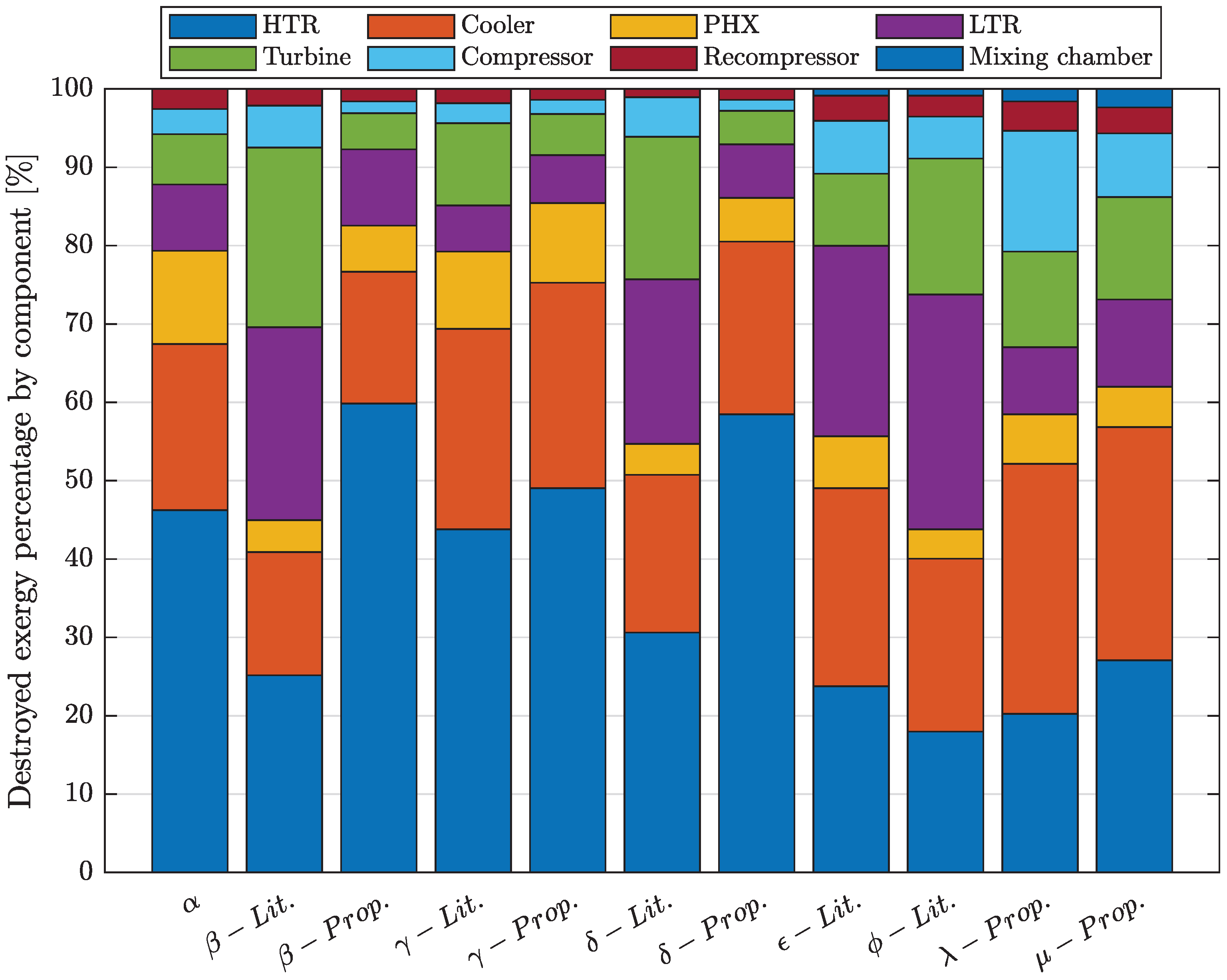
3.6. Exergy Destruction

Quantifying the irreversibilities associated with the cycle off-design operation provides insight into the mechanisms responsible for decreasing its conversion efficiency. In this sense, Figure 8 shows the destruction of physical exergy by cycle configuration and its components at different key points. Analyzing Figure 8, it is possible to verify that the proposed cycle always destroys less exergy than the literature cycle. Moreover, the total exergy destroyed varies little with the net power output for the literature cycle, which, in all the scenarios analyzed, is higher than 8500 $\mathrm{k}$$\mathrm{W}$; however, for the proposed cycle, it reaches as low as 5000 $\mathrm{k}$$\mathrm{W}$ at $\beta$. The exergy destroyed increases when decreasing the net power output for the literature cycle (points $\alpha \stackrel{}{\to }\beta$, $\gamma \stackrel{}{\to }\delta$, and $ϵ\stackrel{}{\to }\varphi$); the opposite effect is observed for the proposed cycle (points $\alpha \stackrel{}{\to }\beta$, $\gamma \stackrel{}{\to }\delta$, and $\lambda \stackrel{}{\to }\mu$).

Since point $\alpha$ corresponds to the design conditions, operating in such a scenario minimizes the exergy destroyed on a per-unit-power-generated basis. Operation at point $\alpha$ is followed by the proposed cycle and then the literature cycle, with the scenarios in which the latter outputs 9 $\mathrm{M}$$\mathrm{W}$ yielding the worst results.

Figure 9 presents the exergy destroyed by each component normalized by the total, providing further insight into the distribution of the exergy destruction. The HTR is the component where most exergy is destroyed under nominal operation. This holds for most scenarios, except for the turbine at points $ϵ$ and $\varphi$ and the cooler at points $\lambda$ and $\mu$. The mixing chamber contributes noticeably percentage-wise to the proposed cycle; however, this is due to the lower total exergy destruction and not because the mixing chamber is an important source of irreversibility.

3.7. Yearly Simulation

Table 6. Yearly simulation summary.

Metric	Literature	Proposed
Availability [%]	76.45	93.45
${\eta }_{season}$ [%]	29	39
${\eta }_{ex,season}$ [%]	48	65
Time 3 out of 3 [%]	0.76	36.24
Time 2 out of 3 [%]	49.93	57.20
Time 1 out of 3 [%]	25.75	0.00
Time unavailable [%]	23.55	6.55

summarizes the results of the yearly simulation for both cycles. It shows how the proposed cycle outshines the literature cycle when considering dispatch curves and shifting cycle low temperatures. The proposed cycle has high availability of 93.45%, representing a strong result when considering renewable energy sources. Nevertheless, it must be stated that the solar multiple of 4 and 12 h of storage considered represents a configuration with high investment costs.

The seasonal efficiencies describe that two cycles with the same design efficiency of 48.3% can substantially vary their effective efficiencies during the year. Varying the cycle’s first-law efficiency from 48.3% to 39% is not desirable, yet it is close to half the drop in efficiency observed for the literature cycle. The literature cycle’s first-law efficiency decreased from 48.3% under nominal operation to 29% under seasonal operation.

Regarding the seasonal exergy efficiency, as the exergy analysis was carried out from the molten salt perspective, all the irreversibilities in the solar field were not considered. This contributes to explaining why these efficiencies were so high.

4. Conclusions

The main conclusions are summarized as follows:

• Arguably due to the experimental nature of the SNL test loop, Petukhov’s and other correlations proposed in the literature underestimate the pressure drop. Moreover, the model accurately describes the power cycle under nominal conditions when adjusted for the pressure drop. Additionally, Gnielinksi’s correlation accurately describes the heat transfer problem in the s-CO₂ RcBC working at a low pressure of 90 bar;
• The s-CO₂ RcBC with a two-shaft configuration cannot achieve the required flexibility when considering the off-design operation of the literature cycle subjected to the Crucero meteorological data and the dispatch curves. The operational range of the literature is highly limited, especially because of the effect of the shaft blockage phenomenon. Thus, the M out of N system dramatically extended the operational range of both the literature and proposed cycles by delaying the onset of the surge in the compressors. Extending the cycles’ operational ranges to higher ambient temperatures while generating the design net power output still requires further work;
• The 20-point decrease between nominal and seasonal first-law efficiencies reflects the literature cycle’s performance shortcomings. The proposed cycle’s three-shaft system is flexible, which can be appreciated through the greater operational range and seasonal first-law efficiency. The latter is 10 points greater for the proposed cycle than the literature. The synergistic effects of decreasing the cycle’s high-end pressure alongside its mass flow rates as a turndown strategy are demonstrated and quantified. Similar to the literature cycle, the surge and supersonic flow phenomena also limit the proposed cycle’s operational range;
• The exergy analysis finds the HTR component to be the greatest source of irreversibility under design conditions. This evidences improper HTR and LTR sizing.

Future work may address the following:

• The description of the cooler and PHX at off-design conditions;
• The techno-economic feasibility of an M out of N system for the s-CO₂ RcBC;
• The design and optimization of an s-CO₂ RcBC with dispatch curves designed primarily to complement solar photovoltaic.

References

1. REN21. Renewable Energy Data in Perspective; Technical Report; REN21: Paris, France, 2022. [Google Scholar]
2. IRENA. Innovation Outlook Thermal Energy Storage; Technical Report; International Renewable Energy Agency: Masdar City, United Arab Emirates, 2020. [Google Scholar]
3. Bergh, K.V.D.; Delarue, E. Cycling of conventional power plants: Technical limits and actual costs. Energy Convers. Manag. 2015, 97, 70–77. [Google Scholar] [CrossRef]
4. Arias, I.; Cardemil, J.; Zarza, E.; Valenzuela, L.; Escobar, R. Latest developments, assessments and research trends for next generation of concentrated solar power plants using liquid heat transfer fluids. Renew. Sustain. Energy Rev. 2022, 168, 112844. [Google Scholar] [CrossRef]
5. Angelino, G. Carbon Dioxide Condensation Cycles For Power Production. J. Eng. Power 1968, 90, 287–295. [Google Scholar] [CrossRef]
6. Cabeza, L.F.; de Gracia, A.; Fernández, A.I.; Farid, M.M. Supercritical CO2 as heat transfer fluid: A review. Appl. Therm. Eng. 2017, 125, 799–810. [Google Scholar] [CrossRef] [Green Version]
7. Dostal, V.; Driscoll, M.J.; Hejzlar, P. A Supercritical Carbon Dioxide Cycle for Next Generation Nuclear Reactors; MIT-ANP-TR-100; MIT Press: Cambridge, MA, USA, 2004. [Google Scholar]
8. Wu, P.; Ma, Y.; Gao, C.; Liu, W.; Shan, J.; Huang, Y.; Wang, J.; Zhang, D.; Ran, X. A review of research and development of supercritical carbon dioxide Brayton cycle technology in nuclear engineering applications. Nucl. Eng. Des. 2020, 368, 110767. [Google Scholar] [CrossRef]
9. Sarmiento, C.; Cardemil, J.M.; Díaz, A.J.; Barraza, R. Parametrized analysis of a carbon dioxide transcritical Rankine cycle driven by solar energy. Appl. Therm. Eng. 2018, 140, 580–592. [Google Scholar] [CrossRef]
10. de Araujo Passos, L.; de Abreu, S.; da Silva, A. A short-and long-term demand based analysis of a CO2 concentrated solar power system with backup heating. Appl. Therm. Eng. 2019, 160, 114003. [Google Scholar] [CrossRef]
11. Sakalis, G. Investigation of supercritical CO2 cycles potential for marine Diesel engine waste heat recovery applications. Appl. Therm. Eng. 2021, 195, 117201. [Google Scholar] [CrossRef]
12. Duvenhage, D.F.; Brent, A.C.; Stafford, W.H. The need to strategically manage CSP fleet development and water resources: A structured review and way forward. Renew. Energy 2019, 132, 813–825. [Google Scholar] [CrossRef]
13. Atif, M.; Al-Sulaiman, F.A. Energy and exergy analyses of solar tower power plant driven supercritical carbon dioxide recompression cycles for six different locations. Renew. Sustain. Energy Rev. 2017, 68, 153–167. [Google Scholar] [CrossRef]
14. Biencinto, M.; González, L.; Valenzuela, L.; Zarza, E. A new concept of solar thermal power plants with large-aperture parabolic-trough collectors and sCO2 as working fluid. Energy Convers. Manag. 2019, 199, 112030. [Google Scholar] [CrossRef]
15. Battisti, F.; de Araujo Passos, L.; da Silva, A. Performance mapping of packed-bed thermal energy storage systems for concentrating solar-powered plants using supercritical carbon dioxide. Appl. Therm. Eng. 2021, 183, 116032. [Google Scholar] [CrossRef]
16. Battisti, F.; de Araujo Passos, L.; da Silva, A. Economic and environmental assessment of a CO2 solar-powered plant with packed-bed thermal energy storage. Appl. Energy 2022, 314, 118913. [Google Scholar] [CrossRef]
17. Clementoni, E.M.; Held, T.; Pasch, J.; Moore, J. Test Facilities; Elsevier Ltd.: Amsterdam, The Netherlands, 2017; pp. 393–414. [Google Scholar] [CrossRef]
18. Dyreby, J. Modeling the Supercritical Carbon Dioxide Brayton Cycle with Recompression. Master’s Thesis, University of Wisconsin–Madison, Madison, WI, USA, 2014. [Google Scholar]
19. Fuller, R.; Eisemann, K. Supercritical CO2 Power Cycle Symposium Centrifugal Compressor Off-Design Performance for Super-Critical CO2. In Presentation, Supercritical CO2 Power Cycle Symposium; Barber Nichols, Inc.: Arvada, CO, USA, 2011. [Google Scholar]
20. Pasch, J.J.; Conboy, T.M.; Fleming, D.D.; Rochau, G.E. Supercritical CO2 Recompression Brayton Cycle: Completed Assembly Description; Technical Report October; Sandia National Laboratories: Albuquerque, NM, USA, 2012. [Google Scholar] [CrossRef] [Green Version]
21. Jahn, I.; Keep, J. On the off-design performance of supercritical carbon dioxide power cycles. In Proceedings of the Shanghai 2017 Global Power and Propulsion Forum, Shanghai, China, 10–12 July 2017; Global Power and Propulsion Society: Zug, Switzerland, 2017; pp. 1–10. [Google Scholar]
22. Correa, F.; Barraza, R.; Too, Y.C.S.; Padilla, R.V.; Cardemil, J.M. Optimized operation of recompression sCO2 Brayton cycle based on adjustable recompression fraction under variable conditions. Energy 2021, 227, 120334. [Google Scholar] [CrossRef]
23. Delsoto, G.; Battisti, F.; da Silva, A. Dynamic modeling and control of a solar-powered Brayton cycle using supercritical CO2 and optimization of its thermal energy storage. Renew. Energy 2023, 206, 336–356. [Google Scholar] [CrossRef]
24. Liu, M.; Tay, N.S.; Bell, S.; Belusko, M.; Jacob, R.; Will, G.; Saman, W.; Bruno, F. Review on concentrating solar power plants and new developments in high temperature thermal energy storage technologies. Renew. Sustain. Energy Rev. 2016, 53, 1411–1432. [Google Scholar] [CrossRef]
25. de Araujo Passos, L.; de Abreu, S.; da Silva, A. Time-dependent behavior of a recompression cycle with direct CO2 heating through a parabolic collector array. Appl. Therm. Eng. 2018, 140, 593–603. [Google Scholar] [CrossRef]
26. Glassman, A. Miscellaneous Losses. In Turbine Design and Application; NASA: Washington, DC, USA, 1972; p. 390. [Google Scholar]
27. Stodola. Modelling of off-design multistage turbine pressures by stodola’s ellipse. In Proceedings of the Energy Incorporated PEPSE User’s Group Meeting, Richmond, VA, USA, 2–3 November 1983. [Google Scholar]
28. Bravo, C. Optimización de Parámetros de Diseño de una Planta Solar de Concentración para Generación Eléctrica Considerando Distintos Escenarios de Despacho. Master’s Thesis, University of Wisconsin–Madison, Madison, WI, USA, 2018. [Google Scholar]
29. Petukhov, B.S. Heat Transfer and Friction in Turbulent Pipe Flow with Variable Physical Properties. Adv. Heat Transf. 1970, 6, 503–564. [Google Scholar] [CrossRef]
30. Blasius, H. Das Aehnlichkeitsgesetz bei Reibungsvorgängen in Flüssigkeiten. In Mitteilungen über Forschungsarbeiten auf dem Gebiete des Ingenieurwesens; Springer: Berlin/Heidelberg, Germany, 1913; pp. 1–41. [Google Scholar] [CrossRef]
31. Jiang, Y.; Liese, E.; Zitney, S.E.; Bhattacharyya, D. Design and dynamic modeling of printed circuit heat exchangers for supercritical carbon dioxide Brayton power cycles. Appl. Energy 2018, 231, 1019–1032. [Google Scholar] [CrossRef]
32. Mylavarapu, S.K.; Sun, X.; Christensen, R.N.; Unocic, R.R.; Glosup, R.E.; Patterson, M.W. Fabrication and design aspects of high-temperature compact diffusion bonded heat exchangers. Nucl. Eng. Des. 2012, 249, 49–56. [Google Scholar] [CrossRef]
Figure 1. RcBC schematic diagram.
Energies 16 04755 g001
Figure 2. Coupled operational range for the literature cycle with 3, 2, and 1 out of 3 compressors functioning.
Energies 16 04755 g002
Figure 3. Coupled operational range for the proposed cycle with 2 and 3 out of 3 compressors functioning.
Energies 16 04755 g003
Figure 4. Coupled operational ranges comparison and key points.
Energies 16 04755 g004
Figure 5. Ts diagrams at points α and β for the literature and proposed cycles.
Energies 16 04755 g005
Figure 6. Ts diagrams for: both cycles at point α , the literature cycle at point γ , and the proposed cycle at point δ .
Energies 16 04755 g006
Figure 7. Ts diagramsfor: both cycles at point α , the literature cycle at point ϵ , and the proposed cycle at point μ .
Energies 16 04755 g007
Figure 8. Exergy destruction per component.
Energies 16 04755 g008
Figure 9. Percentage exergy destruction by component.
Energies 16 04755 g009