Hybrid Source Multi-Port Quasi-Z-Source Converter with Fuzzy-Logic-Based Energy Management

Abstract

In this paper, a fuzzy-logic-based energy management system and a multi-port quasi-z-source converter that utilizes hybrid renewable energy sources are proposed. The system ensures that each energy source module can be used individually by employing fuzzy logic to define the power modes. This approach also helps to prevent switching losses resulting from the extra switching of the source modules. In addition, the proposed energy management does not have a mathematical model, so its applicability is simple, and it is suitable for different multiple-input topologies. The Mamdani fuzzy inference system can be designed to capture the nonlinear behavior of the system owing to linguistic rules. Moreover, the switching losses of the multiport modules were significantly reduced by adopting the quasi-z-source network to the end of the multiport converter. Furthermore, different errors, such as the root mean square error (RMSE), average squared error (ASE), average absolute error (AAE), average time-weighted absolute error (ATWAE), tracking error (TE), and unscaled mean bounded relative absolute error (UMBRAE), were applied to evaluate the fuzzy logic performance from different perspectives. The simulation results were obtained using MATLAB Simulink, and the experimental results were obtained by connecting the circuit to MATLAB Simulink using an Arduino Due.

1. Introduction

Over the past two decades, renewable energy sources have gained significant importance due to the energy crisis, wars, and environmental factors. Consequently, sustainable systems are required in every industry. Although renewable sources have low levels of output power, different sources can be connected to boost the output power. Multiple input converters have the ability to connect more than one power source to each other. In some specific applications, it is not sufficient to connect multiple sources together, and a direct power flow of each source is required to manage energy circulation under certain conditions. For instance, the power output of a photovoltaic (PV) array is decreased under dark conditions, and it is necessary to add another power source to meet the load demand.

Source type is another parameter to consider. Numerous types of multiple-input converters have been reported in the literature. In [1], the authors explained the combinations and rules of multiple-input converters. Different connection methods for several types of sources are presented in this paper. Some basic rules, such as parallel voltage sources, cannot be connected to each other if the voltage levels are different. Furthermore, for some specific converters, more than one source cannot simultaneously supply power. Nejabathkhah proposed a hybrid input source connected via a novel three-input DC-DC converter [2]. The sources could supply power simultaneously, and a battery could be connected as a source to provide bidirectional power flow. A small-signal model was used to control the sources. In [3], multiple inputs were connected via switches to the load using coupled inductors, and the circuit configuration was simple compared to other converters. However, only one source could transfer energy simultaneously. In [4], the authors proposed a multiple-input topology with a parallel connection via switches. In this paper, all inputs shared an inductor, and active switches had the ability to achieve zero current switching (ZCS) by using the switching strategy presented in the research. In addition, the power flowed in only one direction. In [5], the authors proposed a converter with a galvanically isolated system. It had two bridges on the primary and secondary sides of the transformer, and the power flow was controlled. The current capacities of the sources were equal because of the series connection of the sources [5].

A three-source multiple input converter was proposed in [6]. The converter’s areas of application were in electric vehicles with fuel cells, PV arrays, and battery units. A limitation of the converter was that it had three inputs [6]. A three-port DC-DC converter was proposed in [7]. It had a high step-up ratio with reduced voltage stresses. Moreover, the power was bidirectional and had the ability to charge the battery with the load and other sources. The maximum number of input sources was three [7]. The converter presented in [8] proposed a DC-DC multiport converter with dual active bridges. The modules were connected in a ring-type configuration. One of its advantages was that the structure was bidirectional. The authors in [9] proposed a dual-input dual-output bidirectional multiport DC–DC converter. One of the sources was the battery storage system, which had a low level of voltage stress on the semiconductor switches. However, it had only two inputs, and it is unclear whether MPPT can be achieved from other sources. In [10], the authors proposed a multiport converter with multiple outputs in which the sources can deliver power simultaneously. In the next research study, a non-isolated multiple source converter was presented, and the step-up ratio was higher compared with other non-isolated topologies [11]. In this study, the authors considered the normalized voltage stress on the semiconductors. Moreover, the number of sources could be increased, and the voltage gain increased depending on the source count. The same author proposed a new version of [11] in [12]. The voltage gain in this study was higher, and the component number and voltage stress were decreased when compared with [11]. The power flow could be simultaneous or individual in both references.

Z-source topology can exceed the limitations of traditional V-I source power converters and consists of two x-shaped capacitors and two inductors. Due to the structure, the shoot-through mode is not forbidden, which brings an additional control axis to increase the output voltage without damaging the components [13]. In [14], an improved z-source converter was proposed to decrease z-source converter disadvantages, but it still had a discontinuous input current. In addition, the capacitor voltage and inductor current surge were reduced, and the inrush current was limited. To create a common ground for the z-source topology, a common grounded impedance source converter was explained in [15]. This resulted in low levels of stress on semiconductors and decreased the component sizes, but impedance network capacitors are still too large to achieve high voltages. The authors of [16] proposed a quasi-z-source converter that achieved lower levels of voltage stress on the components and a continuous input current, but it had a lower voltage gain compared with a common-ground impedance source. The converter proposed in [17] offered a new quasi-z-source converter with increased component numbers. The converter exhibited a high boost performance with different combinations. However, this converter had problems, such as large voltage spikes. In [18], the authors proposed a multi-input quasi-Z-source converter that combined different power sources by implementing an auxiliary circuit. However, the operation range was not wide, and the design was not simple. Moreover, the switches were faced with high levels of current stress.

In [19], a comprehensive review of different energy management system strategies is provided, including the key factors, methods, and functions involved. However, experimental tests have not been conducted to demonstrate the system performance under real-world conditions. The authors of several papers, including [20,21,22,23,24], have used fuzzy logic as an energy management system, which has the advantage of not requiring a mathematical model of the system, making it less complex to control. The study in [25] focused on optimizing hydrogen consumption while considering battery degradation. However, the system complexity and application area can limit the feasibility of the proposed energy management system. In [26], a maximum efficiency range recognition-based energy management control system was proposed that controlled fuel cell consumption and power flow between two sources using methods such as the sequential quadratic programming algorithm (SQP) and equivalent consumption minimum strategy (ECMS). However, the estimation of equivalent factors in an ECMS can be influenced by the specific characteristics of the driving cycle being analyzed. In [27], instantaneous optimization and mathematical equations were used to explain the structural assumptions. In addition, the proposed approach may not be easily applicable to situations with stochastic demands, and the authors acknowledged that while the locally optimal solution it provides can be effective, it may not be a globally optimal control policy. In [28], a multi-agent-based energy management system was proposed, with three different levels that each had unique duties. However, as in dealing with complex decision problems, an MAS-based energy management strategy may exhibit inadequate real-time performance in decision making. In [29], adaptive neuro-fuzzy inference systems for power management were introduced using a three-phase inverter as the converter type. However, this approach required datasets from the learning part of the system history. In [30], an adaptive droop control method for power management using batteries, supercapacitors, and fuel cell hybrid sources was proposed, although large-scale operations can pose challenges to this control strategy. In [31], a hybrid power storage system and a model predictive method were used for the control strategy, predicting future output power based on historical data and applying a dynamic algorithm to the management strategy. Attaining high performance through this method requires accurate system models as well as information about future driving conditions. The authors of [32] published a case study for energy management systems that included PV arrays, batteries, and grids as hybrid sources. A traditional DC-DC bidirectional converter was used for the battery pack. However, this system has some disadvantages, such as limited application areas. The sliding-mode energy management strategy was proposed in [33] with the nonlinearity of the double integral. In addition, several technical challenges may arise as a result of connecting renewable sources to the power grid. In [34], finite-time tracking control with external noise and input saturation was presented. A neural network was employed to handle disturbances and failures. Moreover, these parameters could be configured using an adaptive scheme.

This study discusses the fuzzy-logic-based energy management system of a hybrid source multi-port quasi-z-source converter which includes PV, wind turbine, and battery sources. In addition, the mathematical model of the quasi-impedance source multi-port converter, simulations of the entire system, and experimental results are presented. Due to the fuzzy logic, the proposed system can manage energy flow from the sources without complex control algorithms when compared with [25,27,28]. One of the biggest features is the modularity of the power management; in other words, not only can the source number be increased but the source types can also be changed, while references [25,28,31] have fixed numbers of sources. Moreover, by setting up the quasi-z-source network to a multi-port converter, the gain of the output voltage is increased, and the voltage stress of the input module switches is decreased when compared with reference [12]. Furthermore, different performance indexes are used to demonstrate system performance, such as ASE, AAE, ATWAE, RMSE, TE and UMBRAE, as in [34]. A detailed comparison table is also added to the discussion and comparison chapter to provide a better explanation and evaluate the performance.

This study is divided into several chapters. Section 2 discusses the multi-port quasi-z-source converter. Section 3 explains the proposed fuzzy-logic-based energy management system. Section 4 and Section 5 present the simulation and experimental results, respectively. In Section 6, the results are discussed. Finally, conclusions are presented in Section 7.

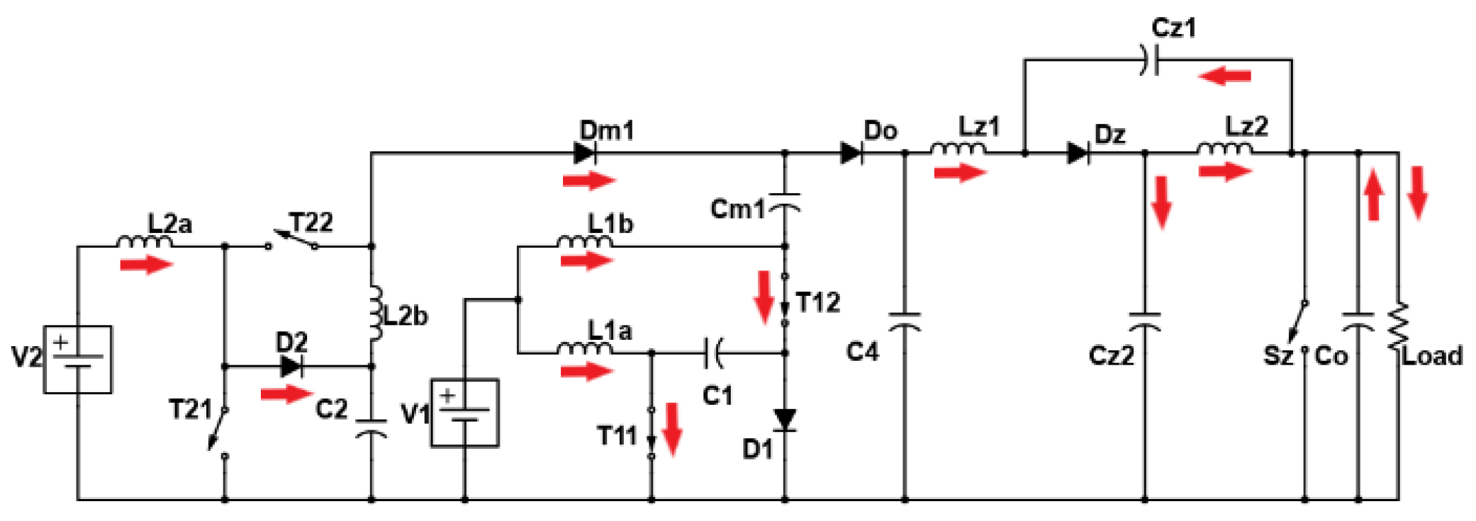
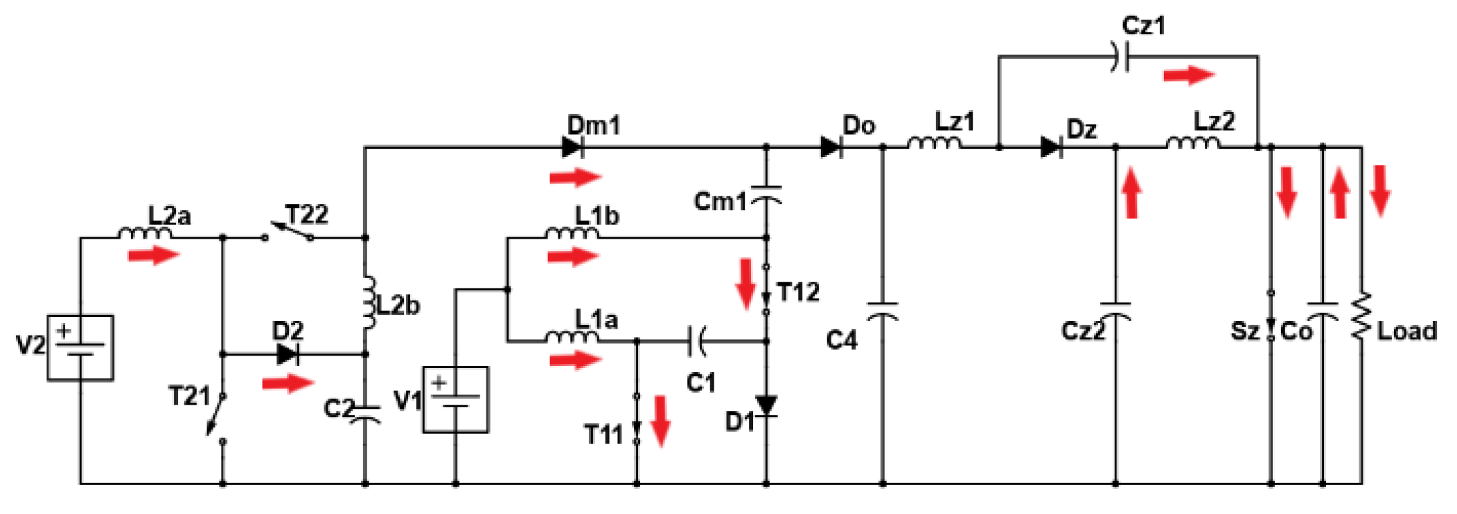
2. Proposed Multi-Port Converter with Quasi-Z-Source Network

A quasi-Z-source network is added to the multiport converter [12], as shown in Figure 1. By adding the quasi-z-source network, the gain of the output voltage is increased using the unique feature of the quasi-z-source, which is the shoot-through mode. Moreover, as a result of the multiport converters, the DC bus voltage decreases, leading to a reduction in the voltage stresses of the multiport converter switches. The number of input sources can be variable and is denoted by n. For simplicity, a two-input scenario is considered. Each module consists of two inductors: a capacitor, diode, and two switches. The modules are connected to each other via a diode and capacitor. A quasi-Z-source network was adopted on the output side. The switches of each module should be turned ON and OFF at their respective times, and the quasi-z-source switch SZ can be switched independently. All the voltage units are volts (V), the current units are amperes (A), the period units are seconds (s), and the frequency units are hertz (Hz)

Working Modes and Mathematical Expressions

Mode 1a (t₀–t₁): In this mode, except for S_z, all of the switches (T12, T11, T22, and T22) are turned ON; this makes D1, D2, and Dm1 reverse-biased, and the quasi-z-source network’s diode, Dz, is forward-biased. Additionally, L1a, L1b, L2a, and L2b are charged by the input sources and capacitor. The quasi-z-source network inductors Lz1 and Lz2 discharge their energy to the output side while at the same time, V_C4 charges the network capacitors Cz1 and Cz2. Waveforms of mode 1a can be seen below in Figure 2. By using Kirchhoff’s voltage law (KVL), the voltages of L1a, L1b, L2a, L2b Lz1, Lz2, and Sz can be expressed using the following formulas, respectively. The red arrows show the direction of the current in each figure of the working mode.

V_L1a = V1

(1)

V_L1b = V1 + V_C1

(2)

V_L2a = V2

(3)

V_L2b = V_C2

(4)

V_Lz1 = V_C4 − V_Cz1

(5)

V_Lz2 = −V_Cz2

(6)

V_Sz = V_Cz1 + V_Cz2

(7)

Mode 1b (t₁–t₂): The switches (T12, T11, T22, and T21) remain in the same position, but the quasi-z-source network switch S_Z is turned on; this makes the diode D_Z reverse-biased. In this state, the inductors Lz1 and Lz2 begin to become charged and store energy while the capacitors Cz1 and Cz2 discharge energy. As S_Z turned ON, the quasi-z-source side of the converter enters the shoot-through mode, which is not forbidden in the z-source topology. The voltages of Lz1, Sz, Lz2, and Dz can be found via the expressions below, applying KVL. Figure 3 shows operation mode 1b.

V_Lz1 = V_Cz2 + V_C4

(8)

V_Sz = 0

(9)

V_Lz2 = V_Cz1

(10)

V_Dz = V_Cz1 + V_Cz2

(11)

Mode 2a (t₂–t₃): Mode de 2a can be seen in Figure 4. The switches of the second module (T22 and T21) are turned OFF, and the diodes D2 and Dm1 become forward-biased. The capacitor of the second module, C2, begins to charge from its input source V₂ and inductor L2a. Moreover, the capacitor C_m1 begins to charge from the second source V₂, L2a, and L2b_. The switch S_Z is not active, and the diode D_Z is forward-biased. The load becomes energized by the inductors Lz1 and Lz2. The equations from (5)–(7) are also valid for this mode. This mode is shown in Figure 4. By applying KVL to the first and second modules separately, the expressions shown below can be obtained.

V_L1a = V1

(12)

V_L1b = V1 + V_C1

(13)

V_L2a = V2 − V_C2

(14)

V_L2b = V_C1 + V_C2 − V_Cm1

(15)

Mode 2b (t₃–t₄): The quasi-z-source switch S_Z is turned ON while the rest of the switches stay in the same position. This mode is shown in Figure 5. The quasi-impedance source network enters a shoot-through state, the network inductors Lz1 and Lz2 are charged by the input source, and the capacitors Cz1 and Cz2 discharge their energy. Equations from (8) to (11) are valid for this condition as well.

Mode 3a (t₄–t₅): In this mode, the switches of the first module (T12 and T11) are turned OFF, while the switches of the second module (T22 and T21) are turned ON. The capacitor C4 is powered by the first input source V1, L1b, and Cm1. The switch S_Z is turned off, and it is in the non-shoot-through mode again. The quasi-z-source part is the same as in modes 1a and 2a, so Equations (5)–(7) are also the same in this mode. Mode 3a can be seen in Figure 6. Finally, the voltages of L2b, L1a, L2a, and L1b can be found using the expressions shown below.

V_L2b = V_C2

(16)

V_L1a = V1 − V_C1

(17)

V_L2a = V2

(18)

V_L1b = V1 + V_Cm1 − V_C4

(19)

Mode 3b (t₅–t₆): The last mode, 3b, is shown in Figure 7. In this mode, the input module switches remain the same while the quasi-z-source network switch is switched ON. The quasi-z-source network enters the shoot-through mode, and Equations (8)–(11) remain the same in this mode.

Calculations can be performed in two parts to make the system understandable: the first part of the calculations includes the multi-port side, and the second part of the calculations includes the quasi-z-source network side. The gain of the first part can be multiplied by the gain of the second part. Using the volt-second balance rule, the inductor voltage over one switching period is 0. Therefore, the inductor voltages of the two input modules can be written as follows to reach the bus voltage V_C4:

V_L1a(t) = 0 = V1d₁ + (V1 − V_C1)(1 − d₁)

(20)

V_C1 = 1/(1 − d₁)V1

(21)

V_L1b(t) = 0 = (V1 + V_C1)d₁ + (V1 + V_Cm1 − V_C4)(1 − d₁)

(22)

0 = V1d₁ + V_C1d₁ + V1 − V_C4(1 − d₁) + V_Cm1(1 − d₁)

(23)

V_C4 = (1/(1 − d₁))V1 + (d₁/(1 − d₁)) + V_Cm1

(24)

V_L2a(t) = 0 = V_C2d₂ + (V2 − V_C2)(1 − d₂)

(25)

=V2d₂ + V2 − V2d₂ − V_C2(1 − d₂)

(26)

V_C2 = 1/(1 − d₂)V2

(27)

V_L2b(t) = 0 = V_C2d₂ + (V_C1 + V_C2 − V_Cm1)(1 − d₂)

(28)

=V_C2d₂ + V_C1(1 − d₂) + V_C2 − V_C2d₂ − V_Cm1(1 − d₂)

(29)

V_Cm1 = V_C1 + 1/(1 − d₂)V_C2

(30)

d₁ and d₂ are the duty cycles of the switches of module 1 and module 2, respectively.

By substituting V_C2 and V_Cm1 into V_C4, the capacitor C₄ voltage of the system can be calculated.

V_C4 = (1/(1 − d₁))V1 + (d1/(1 − d₁)) + V_Cm1

(31)

V_C4 = ((2 − 2d₁ + d₁)/(1 − d₁)²)V1 + (1/(1 − d₂)²)V2

(32)

V_C4 = ((2 − d₁)/(1 − d₁)²)V1 + (1/(1 − d₂)²)V2

(33)

The rest of the calculations are related to the output voltage and quasi-z-source network elements. The shoot-through duty (d_z) cycle can be found in the following expression:

d_z = T_z/(T_z + T_o), T_z = T − T_o

(34)

d_z = Duty cycle of the quasi-z-source switch shoot-through mode.

T_z = Shoot-through period of the quasi-z-source switch, seconds.

T_o = Non-shoot-through period of the quasi-z-source switch, seconds.

T = Period of the quasi-z-source switch.

By using the volt-second balance rule, the voltage of the quasi-impedance source inductors can be calculated for the steady state.

V_Lz1 = 0 = (T₀(V_C4 − V_Cz1) + T_z(V_Cz2 − V_C4))/T

(35)

0 = (1 − d_z)(V_C4 − V_Cz1) + d_z(V_Cz2 − V_C4)

(36)

From V_Cz2 = V_Cz1 − V_C4:

0 = V_C4 − V_Cz1 + d_zV_Cz1 + d_zV_Cz1 − d_ZV_C4

(37)

V_Cz1 = ((1 − d_z)/(1 − 2d_z))V_C4

(38)

V_Lz2 = 0 = (T₀(−V_Cz2) + T_z(V_Cz1))/T

(39)

By subtracting V_Cz1 = V_Cz2 + V_C4:

0 = −V_Cz2 + d_zV_Cz2 + d_z(V_Cz2 + V_C4)

(40)

d_zV_C4 = V_Cz2(1 − 2d_z)

(41)

V_Cz2 = (d_z/(1 − 2d_z))V_C4

(42)

V_Cz1 and V_Cz2 are the voltages of the quasi-z-source network capacitors, and by summing the capacitor voltages, the output voltage can be calculated.

Therefore, using V₀ = V_Cz1 + V_Cz2, we find:

V₀ = ((1 − d_z)/(1 − 2d_z))V_C4 + (d_z/(1 − 2d_z))V_C4

(43)

V₀ = (1/(1 − 2d_z))V_C4

(44)

The waveform of the different parameters can be seen below Figure 8. First module inductor currents i_L1a, i_L2a, capacitor voltages V_C1 and V_C2, quasi-z-source inductor currents i_LZ1 and i_LZ2, quasi-z-source capacitor voltages V_CZ1 and V_CZ2, and quasi-z-source diode current i_DZ can be seen in Figure 8, respectively.

3. Proposed Energy Management Strategy

Hybrid renewable sources with multiple inputs offer distinct advantages over regular power sources. To capitalize on these benefits, wise system planning and power management are required. Fuzzy logic is widely used in various smart applications to achieve higher levels of efficiency owing to its lack of requirements for mathematical modeling, its applicability to nonlinear systems, and its need for only expert guidance [9,10,11,12,13]. The classical fuzzy logic strategy consists of three levels: fuzzification, fuzzy inference, and defuzzification. During the fuzzification process, the knowledge database enters the system and converts the data into fuzzy linguistic variables. The next step is fuzzy inference, when the rules are defined. The final step is defuzzification, in which the fuzzy linguistic variables are converted into understandable values. Figure 9 shows a flowchart that defines the process priorities and logic of energy management systems. According to the flowchart, the powers of the parameters are defined in the first step, and the parameters are then processed. The battery is compared with the simultaneous output power (Pdemand = Pout) in the first process, and the path is selected depending on the outcome. If the battery cannot supply sufficient power to the output, PV power is added to the battery power, and the sum of the two sources is compared with the simultaneous output power. Depending on the answer to the comparison, the battery state of the charge (SOC) level is checked, and wind power is enabled at both SOC levels. If the sum of the two sources is greater than the simultaneous output power, the (SOC) level is checked, and wind power is enabled depending on the SOC level. If the battery can satisfy the simultaneous output power, the battery SOC level is checked, and other sources are enabled depending on the SOC level.

The Mamdani method was used as the inference method in the proposed system because it is easier to apply and depends on expert definitions. A non-complex system is important for expanding applicability; therefore, this method was selected instead of the Sugeno method. The fuzzy logic controller in the proposed system has four inputs (the power of the PV array and wind turbine, instantaneous load power or demanded power, battery SOC, and output (power mode)). The membership functions were configured according to the power ratings of the inputs and divided into three membership functions: low, medium, and high.

The rules of the system were established based on power levels, with 81 rules requiring individual specifications using if-then rules. Fuzzy logic generates numbers between 1 and 3, including 1 and 3, as the output power modes. Based on the power mode output, the system controller regulates each module by attaching or detaching the sources from the rest of the circuit through the power mode relays. A block diagram of the controller system is shown in Figure 10.

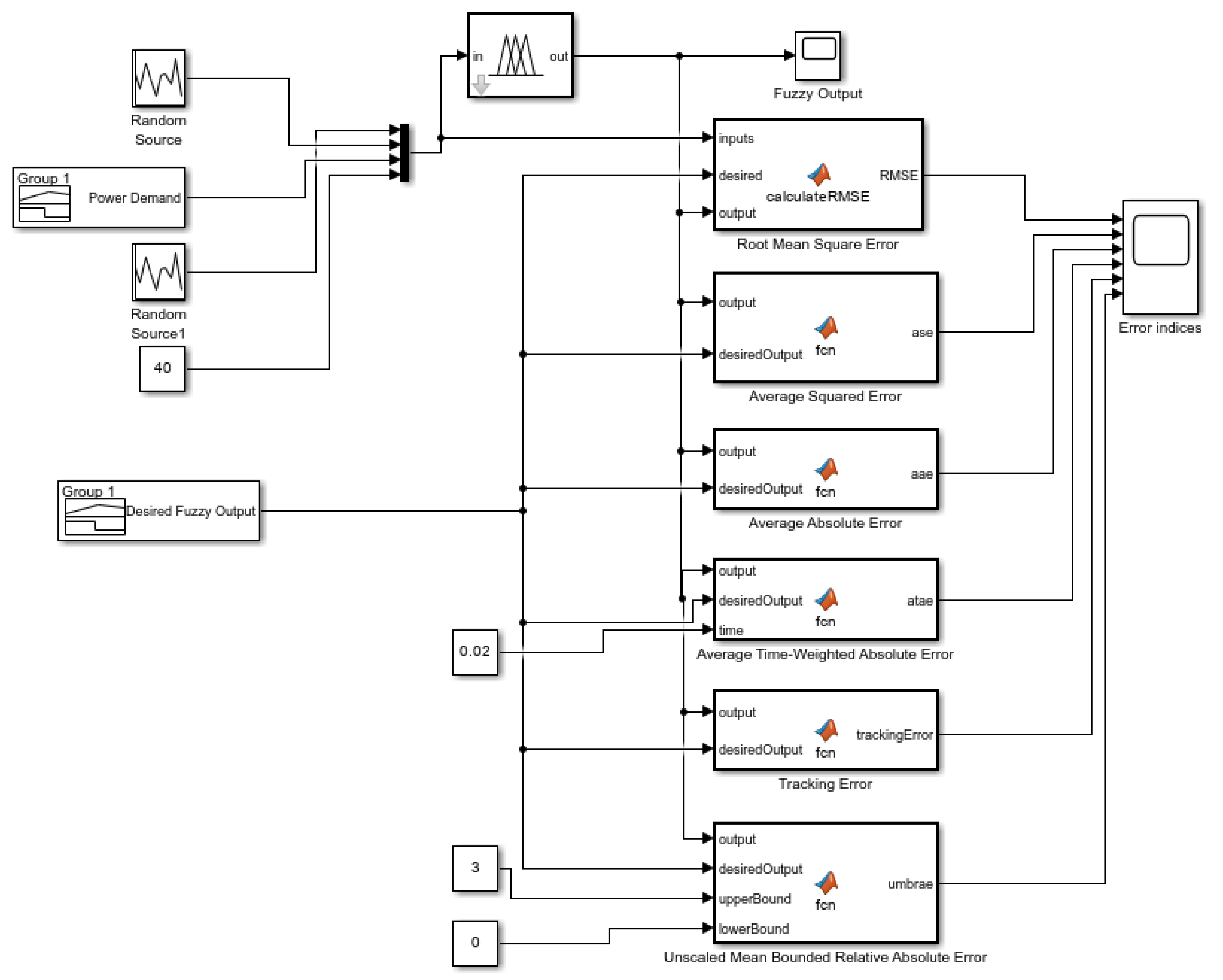
4. Simulation of the Proposed Control System

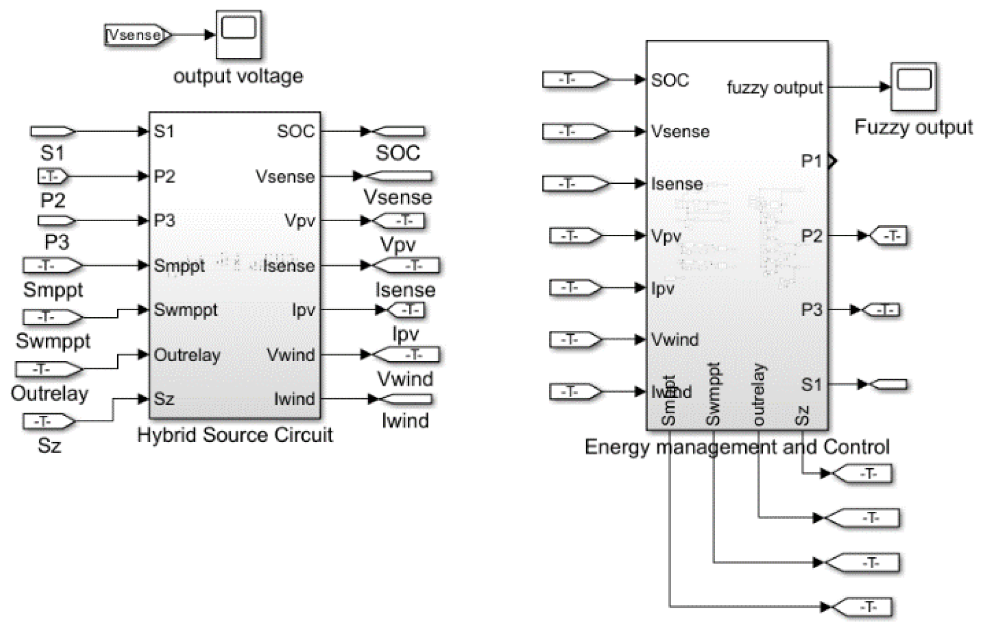
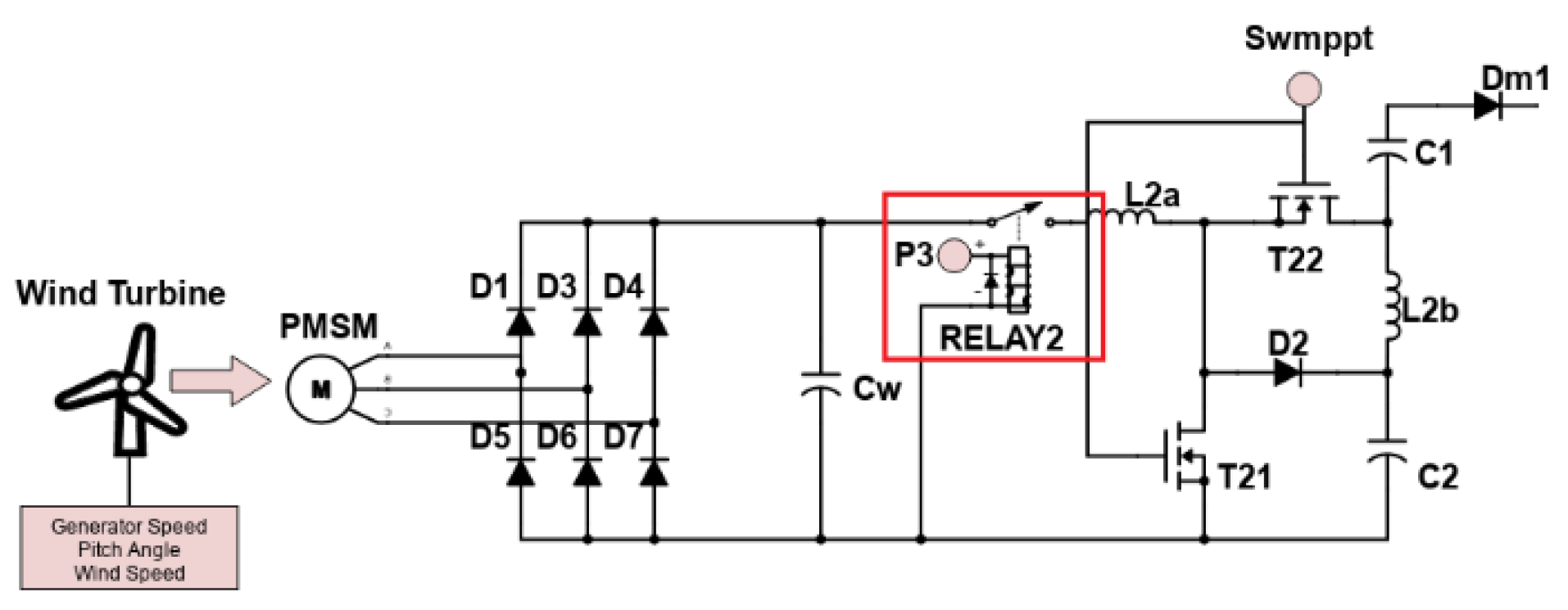
4.1. Simulink Model

MATLAB Simulink was used as a simulation software and was divided into two main sections. The first section is the multi-port converter block where all circuit elements and measurements are performed. The second section is the energy management and control block where the entire control strategy is located. The two main blocks are illustrated in Figure 11. Separating the simulation into two main blocks served two purposes: modularity for the experimental tests and making it more understandable. Three hybrid sources—a battery, PV panel, and wind turbine—were used to perform the simulations and experimental tests. S1, Smppt, Swmppt, and Sz are the switching signals of module 1, module 2, module 3, and the quasi-z-source switch, respectively. S1 is the battery module switching signal, which is the output of the PID controller. Smppt and Swmppt are the PV module and wind module switching signals, respectively, which are the outputs of the MPPT control algorithms. P2 and P3 are the power mode control signals for the PV module relay and wind module relay, respectively. Modules can be attached and detached by controlling relays, and Outrelay is the control signal of the second load relay for the activation of the extra load. SOC, Vsense, Vpv, Isense, Ipv, Vwind, and Iwind are the measurements from the circuit, which are the battery state of charge, output voltage, PV voltage, output current, PV current, wind voltage, and wind current, respectively. The measured parameters were used for the control algorithms and energy management system.

Figure 12 shows the first module of the circuit, the quasi-impedance source part, and the output side of the circuit. The first module is always connected to the quasi-z-source network; however, during fault conditions, it does not supply power to the circuit. The battery should supply power to the system at all times because the rest of the sources are discontinuous. This means that the power supplied by the PV and wind turbine can be interrupted owing to weather conditions. The load was an RL load of 440 Ω and 33 µH. Additionally, according to the scenario, an extra resistive load was connected in parallel to the main load after 0.3 s of the simulation initiation by switching the output relay, which can be seen in the red rectangle in Figure 12. The output power was monitored as the power demanded for the control strategy.

The second module is the PV module, which is attached to the circuit, as shown in Figure 13. The relay attaches or detaches the PV array based on the fuzzy−ogic output, and the relay is shown in red rectangles in Figure 13. The PV array has two inputs that can be adjusted according to irradiance and temperature scenarios.

The irradiance level was set using the signal builder in Simulink, and the level ranged from 0 W/m² to 915 W/m² and then decreased to 530 W/m² after a certain period. The temperature was maintained at 25° Celsius. The specifications of the PV array were obtained from the experimental kit’s “Deneysan YE–1050” datasheet and are listed in

Table 1. PV Array specifications.

Open-circuit voltage VOC (V)	22.77 V
Short-circuit current ISC (A)	5.86 A
Voltage at maximum power point Vmp (V)	18.3 V
Current at maximum power point Imp (A)	5.5 A

.

The third module is the Wind Turbine module, which provides mechanical input to the permanent magnet synchronous machine (PMSM) to obtain a Simulink model of the wind turbine. The PMSM has a three-phase output which is converted into a DC form with three-phase bridge rectifiers. Module 3 is shown in Figure 14, and the module specifications were taken from the experimental kit’s “Deneysan YE–1050” datasheet. The second relay was controlled according to the fuzzy output and is shown by the red rectangle in Figure 14.

Energy management was performed using the Mamdani fuzzy logic method. The MATLAB fuzzy logic designer toolbox was used to configure the system. The fuzzy logic system has four inputs: the power of the PV array, wind turbine, instantaneous load power (demanded), and the battery SOC. The power mode is the output of the fuzzy logic controller. The fuzzy logic designer toolbox is illustrated in Figure 15. All membership functions were defined according to power ratings.

The rules of the system were set after specifying the membership functions. There were 81 rules in the system. The rule editor can be seen in Figure 16, and a detailed rule list can be seen in Appendix A. All these possibilities are considered to provide precise results. Based on the membership functions and rules, the dynamic reaction of the fuzzy logic controller can be viewed in the surface viewer of the fuzzy logic toolbox, as shown in Figure 17.

The membership functions for descriptors can be defined with a straight-line formula, which is:

(y₂ − y₁)/(x₂ − x₁) = (y − y₁)/(x − x₁)

(45)

where y = µ, x = x_T.

y is the membership function, and x is the input variable; thefore, the membership function can be expressed as:

µ = (((y₂ − y₁)(x − x₁))/(x₂ − x₁)) + y₁

(46)

By using the membership function formula, each membership function of the inputs can be expressed one by one:

For PV:

µ_L = (4 − x_PV)/4 [0, 4]

(47)

µ_M = (x_PV − 4)/8 [4, 12]

(48)

µ_M = ((12 − x_PV)/53) − 53 [12, 65]

(49)

µ_H = (x_PV − 65)/25 [65, 80]

(50)

For wind:

µ_L = (1 − x_W)/130 [0, 130]

(51)

µ_M = (x_W − 110)/90 [110, 200]

(52)

µ_M = ((200 − x_W)/80) − 1 [200, 280]

(53)

µ_H = (x_W − 260)/140 [260, 400]

(54)

For the demanded power:

µ_L = (1 − x_d)/35 [0, 25]

(55)

µ_M = (x_d − 35)/25 [35, 60]

(56)

µ_M = ((60 − x_d)/50) + 1 [60, 110]

(57)

µ_H = (x_d − 110)/290 [110, 300]

(58)

Finally, for the SOC:

µ_L = (1 − x_SOC)/290 [0, 25]

(59)

µ_M = (x_SOC − 25)/25 [25, 50]

(60)

µ_M = ((50 − x_SOC)/25) + 1 [50, 75]

(61)

µ_H = (x_SOC − 75)/25 [75, 100]

(62)

By using membership formulas and rules, the exact result of the output can be obtained using the weighted average method. The weighted average method is a widely utilized defuzzification method that is considered relatively simple and is expressed as follows:

$$\mathrm{x}* = (\sum {\mathsf{\mu }}_{\mathrm{n}}(\overline{{\mathrm{x}}_{\mathrm{n}}})·\overline{{\mathrm{x}}_{\mathrm{n}}})/\sum {\mathsf{\mu }}_{\mathrm{n}}(\overline{{\mathrm{x}}_{\mathrm{n}}})$$

(63)

$$\mathrm{x}* = (({\mathsf{\mu }}_{\mathrm{x}1}·\overline{{\mathrm{x}}_1})+ ({\mathsf{\mu }}_{\mathrm{x}2}·\overline{{\mathrm{x}}_2}) + ({\mathsf{\mu }}_{\mathrm{x}3}·\overline{{\mathrm{x}}_3}) + ({\mathsf{\mu }}_{\mathrm{x}4}·\overline{{\mathrm{x}}_4}))/\left({\mathsf{\mu }}_{\mathrm{x}1}+ {\mathsf{\mu }}_{\mathrm{x}2}+ {\mathsf{\mu }}_{\mathrm{x}3}+ {\mathsf{\mu }}_{\mathrm{x}4}\right)$$

(64)

x* is the defuzzied value, and $\overline{{\mathrm{x}}_1}$ and $\overline{{\mathrm{x}}_2}$ are the centroids of the trapeziums, which are reflections of the inputs to output. As a result, by using the above formulas, any conditions of the rules can be calculated.

4.2. Other Control Parameters

The switches were controlled using different methods depending on the type of source, and the control methods are shown in Figure 18. For the battery module (T₁₁ and T₁₂) and quasi-z-source part (S), closed-loop proportional integral derivative (PID) controllers were used. The reference output voltage is compared with the measured output voltage, and the resulting error is inputted into a proportional integral derivative (PID) block. The output of the PID block is the duty cycle (DC) of the semiconductor switch, and the relational operator compares the duty cycle and repeating sequence at a fixed frequency to convert the number of duty cycles into a square-wave waveform. The different numbers show the input and output port numbers of the Simulink block.

Owing to their characteristics, the PV array and wind turbine must be examined separately to obtain their maximum power points (MPPs). One of the MPP methods is the perturb and observe method, which has been applied to track the MPP, as shown in Figure 18. The perturb and observe method has an initial duty cycle which increases or decreases by a delta value according to the dV and dP values. The dV and dP values represent the differences between the instantaneous voltage/power and old voltage/power, respectively.

Moreover, there are maximum and minimum limits to the desired duty cycle. The perturb and observe method outputs the duty cycle number, which is then input into the pulse width modulation (PWM) generator to produce the waveform for the switches of the modules. To achieve closed-loop control, an additional control parameter had to be added at the end of the PWM generator, which took the output voltage and compared it with the reference output voltage.

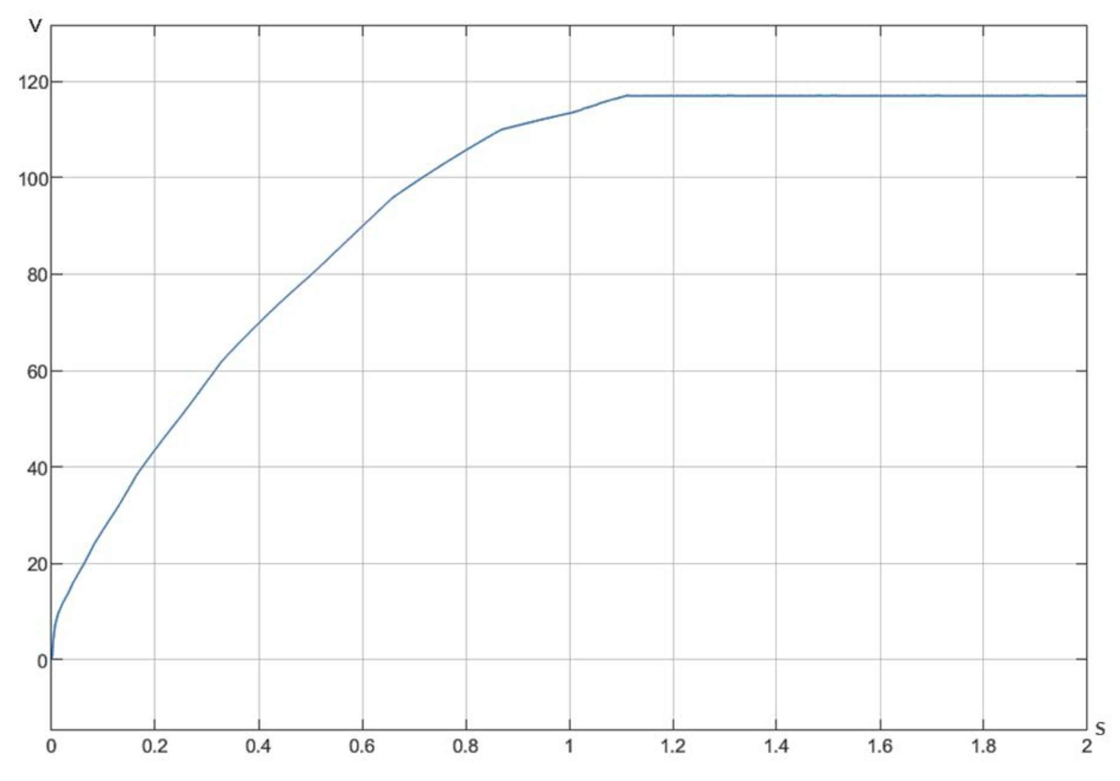
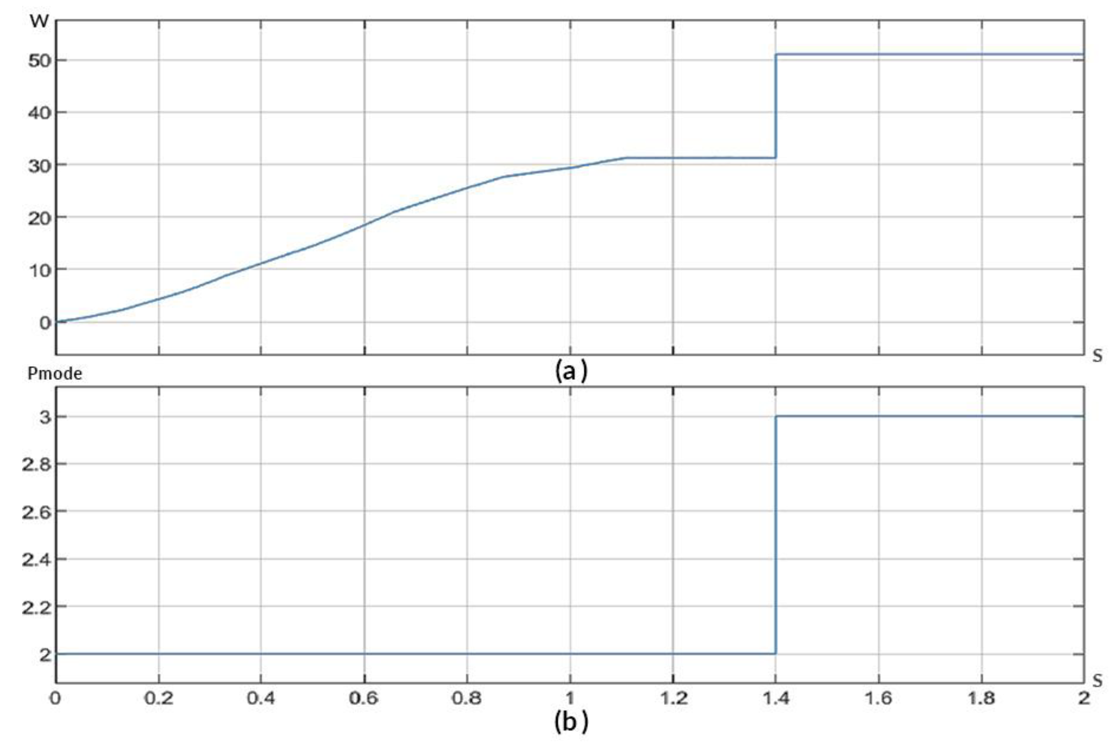
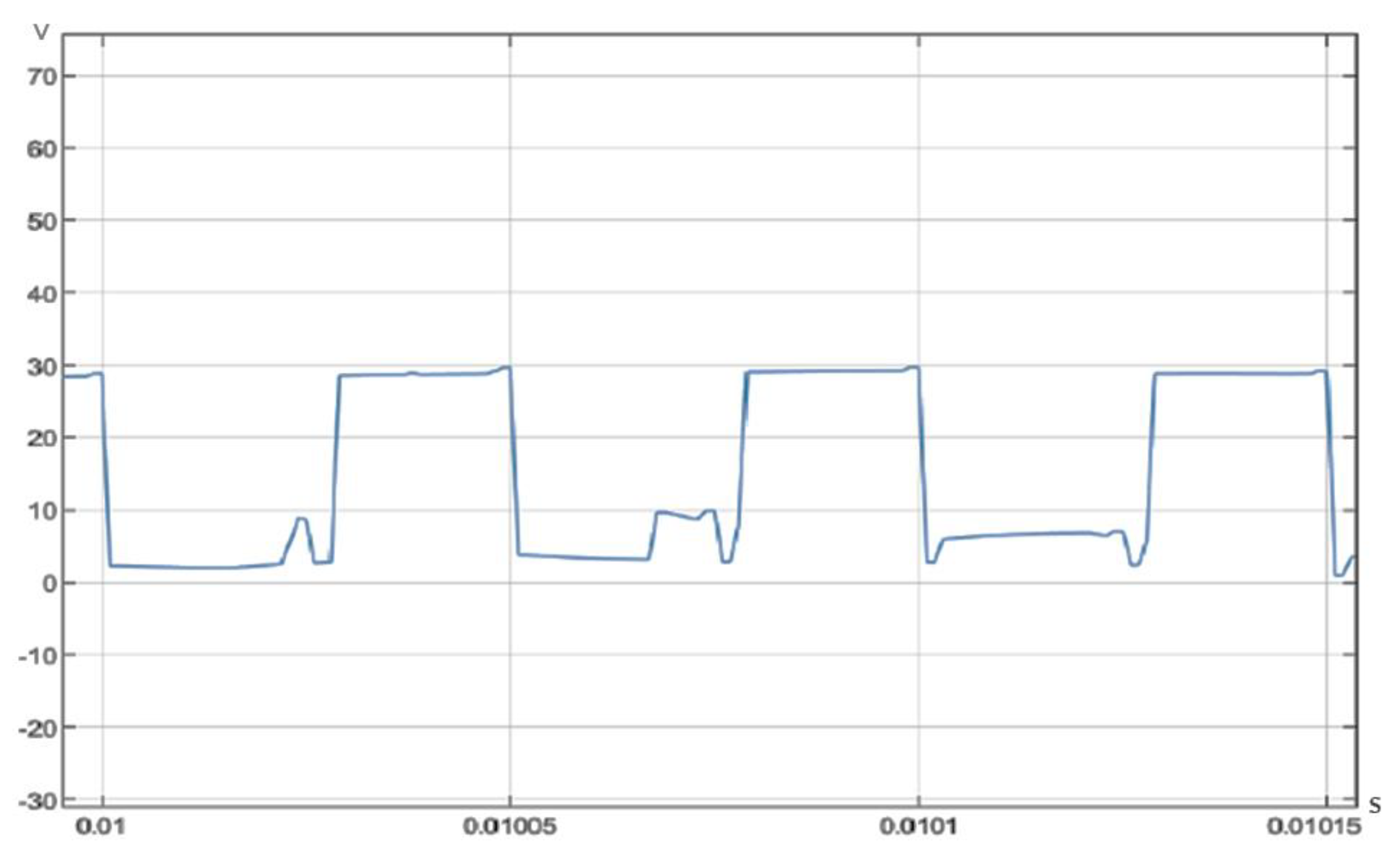
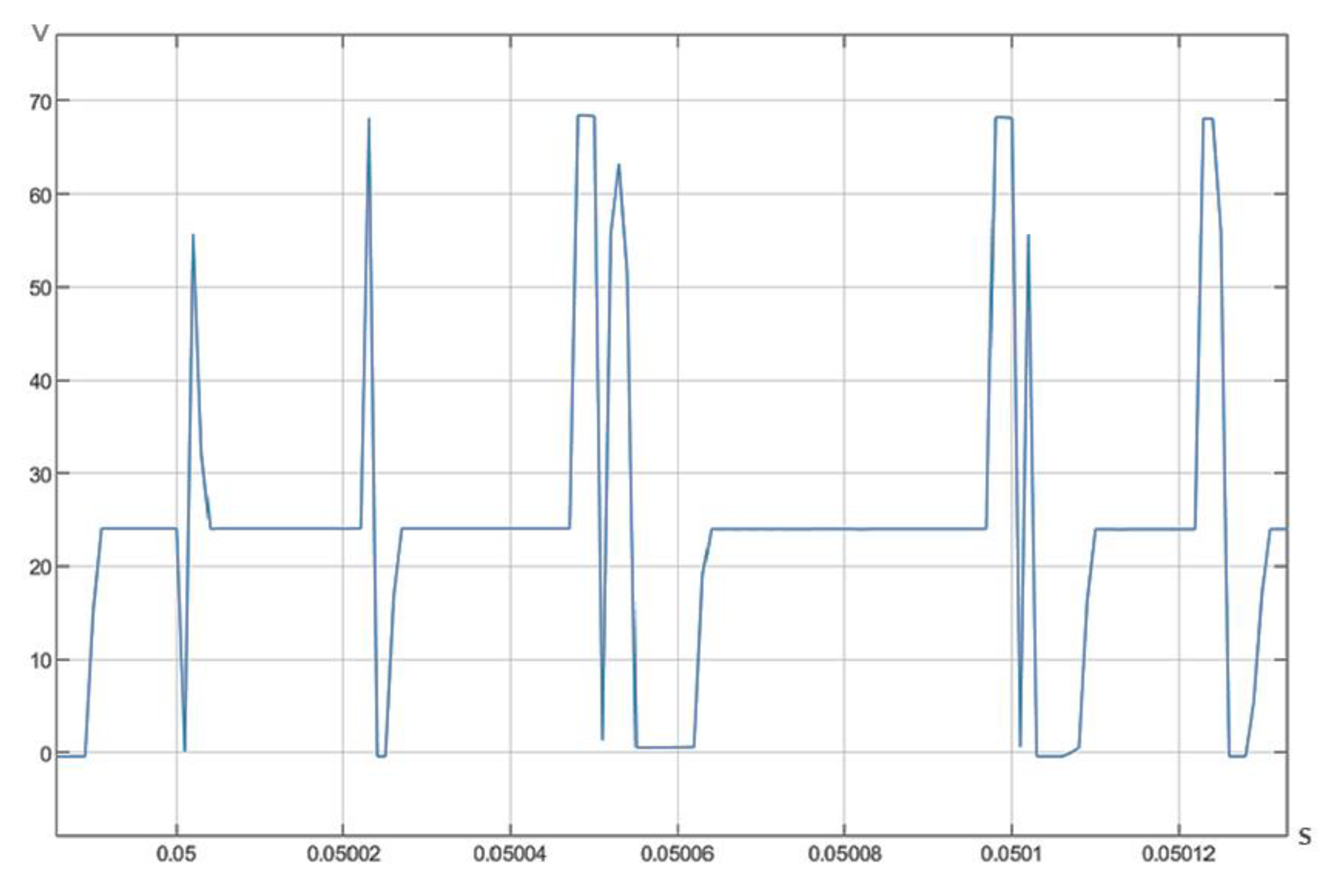
4.3. Simulation Results

The simulation duration was 2 s, and the step change in the load was 1.4 s. The duration of the simulation was chosen as 2 s because the duration to reach the desired output voltage was 1 s, and based on the duration of the simulation, the step change was decided to be 1.4 s. The main reason for the simulation duration was to demonstrate the transition from the transient state to the steady state. According to the first scenario, the battery SOC was 40%, and the converter reached the target output voltage at 1.08 s. During the step change, there were no changes in the output voltage, as shown in Figure 19. When the battery SOC was 40%, the fuzzy output started in mode 2, and at the step change, the instantaneous power increased up to 52 watts. Simultaneously, the fuzzy output changed the mode from 2 to 3, as shown in Figure 20. An important point to note is that at the beginning, all sources were activated by the control system until the voltage reached up to 115 V. This logic was intended to help the output voltage reach the desired level as soon as possible.

In the second scenario, the battery SOC was 95%, and the output voltage reached the target almost at the same time as in the previous case, thanks to the starting strategy of the control system, as shown in Figure 21. In Figure 22, depending on the power levels of the sources, the fuzzy output started with power mode 1, and at the load changes, the power mode switched to mode 2. After several microseconds, even though the power was increased, there were no changes in the power mode depending on the SOC level and the PV power.

A voltage stress comparison of the switches is shown in Figure 23 and Figure 24. The first module’s switch T₁₂ is compared with a quasi-impedance source network, and without a quasi-impedance source network, the voltage stress with the quasi-z-source network is approximately 15 V. In addition, the voltage stress of semiconductor switch T₁₂ without the quasi-z-source network has a peak of approximately 30 V under the same conditions. The quasi-z-source network delays the output voltage to reach the target value of 120 V, which is around 1.1 s, but there is a large difference in the voltage stress. This is because the voltage gain of the multi-port side does not need to be high, and the quasi-z-source network has a higher gain, which lowers the voltage stresses of the switches on the multi-port side.

The voltage stress difference between the two configurations increases at higher voltages. For the multi-port quasi-impedance source network, the voltage stress of switch T12 remains at 19 V when the output voltage reaches its desired value, as shown in Figure 25. In addition, for the multi-port without a quasi-z-source case, the voltage stress of switch T12 at the desired output has a 68 V peak, as can be seen in Figure 26. Both waveforms have different timings because the output voltages reach 120 V at different times.

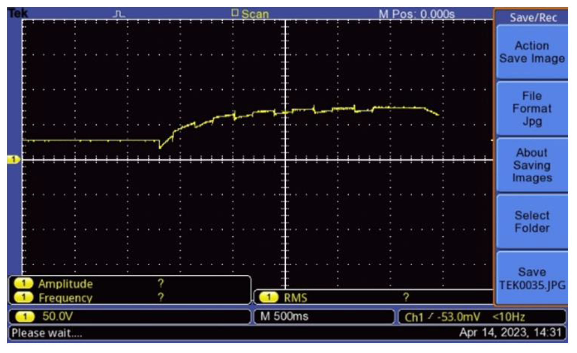
5. Experimental Test

The experimental tests consisted of several sections, such as component selection, printed circuit board (PCB) layout design, PCB component assembly, and measurements. Arduino is an embedded platform that can be programmed to generate signals, read analog values, or connect different devices. The Arduino DUE was selected as the main controller for the experiments because it can be connected to MATLAB Simulink and is suitable for the process. Additionally, several configurations were required to enable the use of the Arduino platform in MATLAB Simulink. For example, the MATLAB Support package for Arduino hardware must be installed from the add-on explorer.

During the experimental tests, the DENEYSAN YE-1050 experiment kit’s PV array, wind turbine, and battery were used to obtain power. The ACS712 current sensor was used for current measurements, but it could not be connected directly to an Arduino DUE because the ACS712 current sensor has a 5 V analog output signal, while the Arduino DUE has a maximum 3.3 V analog input. Therefore, the ACS712 current sensor was connected to an Arduino UNO, which communicated with a digital-to-analog converter to send the read current value to the Arduino DUE. Voltage divider resistors were used to measure the voltages and calculate the power (voltage multiplied by current). This process is illustrated in Figure 27. Before multiplying the voltage and current, the voltage-resistor formula was applied to calculate the actual measured voltage. Different numbers show input port of the block.

Table 2. Component values.

Components	Values
L1a, L2a, L1b, L2b, L3a, L3b	100 µH
C1, C3	47 µF
C2	470 µF
Cm1, Cm2	470 µF
Co	680 µF
CPV, CWind	470 µF
CZ1, CZ2	33 µF
LZ1, LZ2	100 µH
Load 1	440 ohm, 33 µH
Load 2	680 ohm

shows the component values of the proposed converter.

During the design of the PCB layout, the traces had to be wide enough to handle the current and voltage. According to IPC-2221 regulations, the amount of current can be calculated using the following formula:

A = (T × W × 1.378[(mils/oz)/(ft)²]

(65)

A = Area of the trace.

T = Trace thickness.

W = Trace width.

I_MAX = ((k × T_RISE^b) × A^c) [Ampere]

(66)

T_RISE = Maximum desired temperature in Celsius.

K = Constant for external layers; k = 0.048, for internal layers; k = 0.024.

T_RISE = Maximum desired temperature rise, A (ampere).

b = Constant, 0.44.

c = Constant, 0.725.

Experimental Results

A laboratory environment was used to perform the experimental tests in March, and the temperature, humidity, and other factors were stabilized. The experimental configurations were the same as the simulation configurations, and the results are shown in the figures below. Waveforms were obtained as experimental results via an oscilloscope with 50 V/div and 500 ms/div. Moreover, the current measurements were directly taken from the ACS712 current sensor via the Arduino UNO, sent to the Arduino DUE via the DAC, and reflected in MATLAB Simulink. Therefore, MATLAB Simulink scopes showed the live data obtained from the current sensor. As explained previously, these measured values are multiplied by the voltage to obtain the power values, and the results are shown in Figure 28 and Figure 29.

In the first scenario, the battery SOC was 40%, and the desired output voltage was reached at the desired output voltage in 1 s. After reaching the target, the PID corrected and stabilized the output voltage. The second load was activated at 1.4 s, and there were no changes in the output voltage, finally, the test was completed at 2. The voltage then began to drop, and it can be seen in Figure 28.

In the second scenario, the battery SOC level was 90%, and the target output voltage reached the desired level in 1 s. The PID made corrections and stabilized the output voltage to the desired level, and the output voltage is shown in Figure 30.

The SOC level of the battery plays a significant role in the starting point of the power mode. The system has the capability to meet the load demand at the starting point and depending on the power ratings, it changes after 1.4 s. Depending on the measurements of all the sources, the energy management system decides to activate all of the sources when the load demand increased. Therefore, the energy management system started with power mode 1 and switched to power mode 3 when the second load is activated. The power level and power mode can be seen in Figure 31.

Several analyses were performed to evaluate the performance of the fuzzy-logic-based energy management control strategy. The RMSE, ASE, AAE ATWAE, TE, and UMBRAE indexes were evaluated in MATLAB Simulink, and the results are shown in the Figure 32. The reason for using different indexes is that the error indexes have different purposes and provide distinct insights into the system performance. For example, the RMSE is an index frequently used to determine the overall goodness of fit or accuracy of a system, whereas the AAE provides a measure of the average magnitude of the errors regardless of their direction. Indices are different colors in Figure 32. RMSE, AAE, and ATWAE are purple lines, ASE is an orange line, TE is a green line, and UMBRAE is a blue line. This is normal for some of the errors that are the same under certain circumstances because the output and desired output values are close to each other.

In addition, random sources were added as inputs of the fuzzy logic to make noise and can be seen in Figure 33. The errors are close to 0, which is good for the system performance. The performance of the fuzzy logic system is good because the errors are close to 0 and to each other.

Figure 34 shows the C_z2 voltage of the quasi-impedance source network, the voltage is only around 75 V which is carrying less voltage stress.

6. Discussion and Comparison

The simulation and experimental results are the same. The only difference between the simulation and experimental tests is the fuzzy slope. However, this difference is so small and does not affect the result, so it can be neglected. In this section, the differences and comparisons will be discussed.

The difference is the slope of the fuzzy logic output. The slew rate of the fuzzy output is 0 in the simulations. On the other hand, in the real world, there are delays and tolerances; therefore, the slope can be predictable but may also be neglected because it does not affect the result. In addition, MATLAB Simulink configuration can be another reason. Other than this, the reactions of the fuzzy logic output of both the simulation and experimental tests are similar.

The system parameters can be set to adapt to different applications, and better performance can be obtained by configuring parameters, such as the PID parameters, or by switching the frequencies of the semiconductor switches. The switching frequency can be set lower to decrease the switching losses, but this causes a decrease in the output voltage. Therefore, the frequency can be lowered for applications in which a lower voltage is required. Furthermore, the PID parameters can be tuned using different methods. The PID parameters were set using a trial–error method in the simulation and experimental tests. However, MATLAB Simulink has an auto-tuning system to configure the PID parameters. Therefore, better performance can be obtained using autotuning methods.

The experimental setup is shown in Figure 35. In Figure 35, the multiport quasi-Z-source can be seen in a blue rectangle on the PCB, the load side can be seen in a green rectangle and finally, the Arduino Uno, Arduino DUE, and the digital-to-analog converter can be seen in red rectangles.

Table 3. Comparison of the different energy management references and proposed energy management strategy.

Reference	Adv./Disadv.	Response Time	Complexity	No. of Inputs
[25]	Fuel economy is good; system durability is high; complex system, limited application area.	−	High	Three inputs (fuel cell, battery, and super capacitor),
[27]	Reasonable assumptions; complex system.	+	High
[28]	Long decision-making time; complex system.	−	High	Three inputs (PV, wind turbine, and battery).
[29]	Hybrid sources; needs datasets.	+	Medium	Five inputs (grid, PV, wind turbine, fuel cell, and battery).
[31]	Can predict the future; large-scale operations are difficult; needs datasets.	+	Medium	Two inputs (LTO, Li-Ti-O battery; NCM, Ni-Co-Mn battery).
Proposed System	No mathematical algorithm; fuzzy rules; can adapt high number of sources.	+	Low	N numbered (any type of source, including renewable sources).

shows a comparison of the proposed energy management with other research studies from the literature [25,27,28] which have more complex systems, making them less attractive. In addition, the proposed energy management strategy has no mathematical algorithm and is rule-based; therefore, experts can easily adapt the energy management system to a larger number of sources. Moreover, the referenced studies [29,31] required data sets from the history. Additionally, the proposed system requires only the fuzzy rules, which are defined by the user. The study in [33] can face technical problems as renewable sources are connected. However, the proposed system can accept any type of source by implementing control algorithms based on the source type. The PID control algorithm is applied to the first module, which is battery connected, and different MPPT algorithms are applied to the second and third modules, which have PV and wind sources, respectively.

7. Conclusions

The proposed energy management system and multi-port quasi-z-source converter were presented, simulated, and tested under various conditions, including load changes. The results show that the simulation and experimental tests match each other, indicating the effectiveness of the proposed system. The system can be adapted to different systems by simply changing the parameters, making it suitable for both simulations and real-world applications. This feature is important because it makes the system usable and attractive. Furthermore, the simultaneous power flow from multiple sources can feed the load side, and more power sources can be added to the system if required. The voltage gain and output power can be increased by adding additional power sources to the system. Therefore, the proposed system can be used in high-voltage and high-power applications. In addition, the voltage stresses on the switches of the multi-port side are significantly reduced with the quasi-z-source network. In future work, attention can be paid to battery charging and the overall system efficiency to improve the sustainability of the management system. Moreover, to decrease the computational burden of fuzzy rules, different fuzzy-based control topologies can be adopted for the system.

References

1. Li, Y.; Yang, D.; Ruan, X. A Systematic Method for Generating Multiple-Input DC/DC Converters. In Proceedings of the 2008 IEEE Vehicle Power and Propulsion Conference, Milan, Italy, 23–27 October 2023; IEEE: New York, NY, USA, 2008; pp. 1–6. [Google Scholar]
2. Nejabatkhah, F.; Danyali, S.; Hosseini, S.H.; Sabahi, M.; Niapour, S.M. Modeling and Control of a New Three-Input Dc-Dc Boost Converter for Hybrid PV/FC/Battery Power System. IEEE Trans. Power Electron. 2012, 27, 2309–2324. [Google Scholar] [CrossRef]
3. Argentini, S.; Pietroni, I.; Mastrantonio, G.; Viola, A.; Zilitinchevich, S. Characteristics of The Multiple-Input DC-DC Converter. In Proceedings of the IEEE Power Electronics Specialist Conference PESC ’93, Seattle, WA, USA, 20–24 June 1993; pp. 115–120. [Google Scholar]
4. Dobbs, B.G.; Chapman, P.L. A Multiple-Input DC-DC Converter Topology. IEEE Power Electron. Lett. 2003, 1, 6–9. [Google Scholar] [CrossRef]
5. Karthikeyan, V.; Gupta, R. Multiple-Input Configuration of Isolated Bidirectional DC–DC Converter for Power Flow Control in Combinational Battery Storage. IEEE Trans. Ind. Inform. 2018, 14, 2–11. [Google Scholar] [CrossRef]
6. Ahrabi, R.R.; Ardi, H.; Elmi, M.; Ajami, A. A Novel Step-Up Multiinput DC–DC Converter for Hybrid Electric Vehicles Application. IEEE Trans. Power Electron. 2017, 32, 3549–3561. [Google Scholar] [CrossRef]
7. Dezhbord, M.; Mohseni, P.; Hosseini, S.H.; Mirabbasi, D.; Islam, M.d.R. A High Step-Up Three-Port DC–DC Converter with Reduced Voltage Stress for Hybrid Energy Systems. IEEE J. Emerg. Sel. Top. Ind. Electron. 2022, 3, 998–1009. [Google Scholar] [CrossRef]
8. Nazih, Y.; Abdel-Moneim, M.G.; Aboushady, A.A.; Abdel-Khalik, A.S.; Hamad, M.S. A Ring-Connected Dual Active Bridge Based DC-DC Multiport Converter for EV Fast-Charging Stations. IEEE Access 2022, 10, 52052–52066. [Google Scholar] [CrossRef]
9. Jalilzadeh, T.; Rostami, N.; Babaei, E.; Hosseini, S.H. Bidirectional Multi-port Dc–Dc Converter with Low Voltage Stress on Switches and Diodes. IET Power Electron. 2020, 13, 1593–1604. [Google Scholar] [CrossRef]
10. Ninma Jiya, I.; Van Khang, H.; Kishor, N.; Ciric, R.M. Novel Family of High-Gain Nonisolated Multiport Converters with Bipolar Symmetric Outputs for DC Microgrids. IEEE Trans. Power Electron. 2022, 37, 12151–12166. [Google Scholar] [CrossRef]
11. Varesi, K.; Hosseini, S.H.; Sabahi, M.; Babaei, E. Modular Non-Isolated Multi-Input High Step-up Dc-Dc Converter with Reduced Normalised Voltage Stress and Component Count. IET Power Electron. 2018, 11, 1092–1100. [Google Scholar] [CrossRef]
12. Varesi, K.; Hosseini, S.H.; Sabahi, M.; Babaei, E. A Multi-Port High Step-Up DC-DC Converter with Reduced Normalized Voltage Stress on Switches/Diodes. In Proceedings of the 9th Annual International Power Electronics, Drive Systems, and Technologies Conference, PEDSTC 2018, Tehran, Iran, 14–15 February 2018; pp. 1–6. [Google Scholar] [CrossRef]
13. Peng, F.Z. Z-Source Inverter. IEEE Trans. Ind. Appl. 2003, 39, 504–510. [Google Scholar] [CrossRef]
14. Tang, Y.; Xie, S.; Zhang, C. An Improved Z-Source Inverter. IEEE Trans. Power Electron. 2011, 26, 3865–3868. [Google Scholar] [CrossRef]
15. Shen, H.; Zhang, B.; Qiu, D.; Zhou, L. A Common Grounded Z-Source DC–DC Converter with High Voltage Gain. IEEE Trans. Ind. Electron. 2016, 63, 2925–2935. [Google Scholar] [CrossRef]
16. Anderson, J.; Peng, F.Z. Four Quasi-Z-Source Inverters. In Proceedings of the 2008 IEEE Power Electronics Specialists Conference, Rhodes, Greece, 15–19 June 2008; IEEE: New York, NY, USA, 2008; pp. 2743–2749. [Google Scholar]
17. Hosseini, S.M.; Ghazi, R.; Nikbahar, A.; Eydi, M. A New Enhanced-boost Switched-capacitor Quasi Z-source Network. IET Power Electron. 2021, 14, 412–421. [Google Scholar] [CrossRef]
18. Torki Harchegani, A.; Asghari, A.; Jazaeri, M. A New Soft-switching Multi-input Quasi-Z-source Converter for Hybrid Sources Systems. IET Renew. Power Gener. 2021, 15, 1451–1468. [Google Scholar] [CrossRef]
19. Biasini, R.; Onori, S.; Rizzoni, G. A Near-Optimal Rule-Based Energy Management Strategy for Medium Duty Hybrid Truck. Int. J. Powertrains 2013, 2, 232. [Google Scholar] [CrossRef]
20. Petrović, D.J.; Lazić, M.M.; Lazić, B.V.J.; Blanuša, B.D.; Aleksić, S.O. Hybrid Power Supply System with Fuzzy Logic Controller: Power Control Algorithm, Main Properties, and Applications. J. Mod. Power Syst. Clean Energy 2021, 10, 923–931. [Google Scholar] [CrossRef]
21. Ganguly, P.; Kalam, A.; Zayegh, A. Fuzzy Logic-Based Energy Management System of Stand-Alone Renewable Energy System for a Remote Area Power System. Aust. J. Electr. Electron. Eng. 2019, 16, 21–32. [Google Scholar] [CrossRef]
22. Koulali, M.; Mankour, M.; Negadi, K.; Mezouar, A. Energy Management of Hybrid Power System PV Wind and Battery Based Three Level Converter. TECNICA ITALIANA-Ital. J. Eng. Sci. 2019, 63, 297–304. [Google Scholar] [CrossRef] [Green Version]
23. Baset, D.A.-E.; Rezk, H.; Hamada, M. Fuzzy Logic Control Based Energy Management Strategy for Renewable Energy System. In Proceedings of the 2020 International Youth Conference on Radio Electronics, Electrical and Power Engineering (REEPE), Moscow, Russia, 12–14 March 2020; IEEE: New York, NY, USA, 2020; pp. 1–5. [Google Scholar]
24. Teo, T.T.; Logenthiran, T.; Woo, W.L.; Abidi, K.; John, T.; Wade, N.S.; Greenwood, D.M.; Patsios, C.; Taylor, P.C. Optimization of Fuzzy Energy-Management System for Grid-Connected Microgrid Using NSGA-II. IEEE Trans. Cybern. 2021, 51, 5375–5386. [Google Scholar] [CrossRef]
25. Zhang, Z.; Guan, C.; Liu, Z. Real-Time Optimization Energy Management Strategy for Fuel Cell Hybrid Ships Considering Power Sources Degradation. IEEE Access 2020, 8, 87046–87059. [Google Scholar] [CrossRef]
26. Wang, T.; Li, Q.; Wang, X.; Qiu, Y.; Liu, M.; Meng, X.; Li, J.; Chen, W. An Optimized Energy Management Strategy for Fuel Cell Hybrid Power System Based on Maximum Efficiency Range Identification. J. Power Sources 2020, 445, 227333. [Google Scholar] [CrossRef]
27. Kim, N.; Cha, S.; Peng, H. Optimal Control of Hybrid Electric Vehicles Based on Pontryagin’s Minimum Principle. IEEE Trans. Control Syst. Technol. 2011, 19, 1279–1287. [Google Scholar] [CrossRef] [Green Version]
28. Yu, J.; Dou, C.; Li, X. MAS-Based Energy Management Strategies for a Hybrid Energy Generation System. IEEE Trans. Ind. Electron. 2016, 63, 3756–3764. [Google Scholar] [CrossRef]
29. Garcia, P.; Garcia, C.A.; Fernandez, L.M.; Llorens, F.; Jurado, F. ANFIS-Based Control of a Grid-Connected Hybrid System Integrating Renewable Energies, Hydrogen and Batteries. IEEE Trans. Ind. Inform. 2014, 10, 1107–1117. [Google Scholar] [CrossRef]
30. Li, Q.; Wang, T.; Dai, C.; Chen, W.; Ma, L. Power Management Strategy Based on Adaptive Droop Control for a Fuel Cell-Battery-Supercapacitor Hybrid Tramway. IEEE Trans. Veh. Technol. 2018, 67, 5658–5670. [Google Scholar] [CrossRef]
31. Zhang, S.; Xiong, R.; Sun, F. Model Predictive Control for Power Management in a Plug-in Hybrid Electric Vehicle with a Hybrid Energy Storage System. Appl. Energy 2017, 185, 1654–1662. [Google Scholar] [CrossRef]
32. Suthar, S.; Pindoriya, N.M. Energy Management Platform for Integrated Battery-Based Energy Storage—Solar PV System: A Case Study. IET Energy Syst. Integr. 2020, 2, 373–381. [Google Scholar] [CrossRef]
33. Ghosh, S.K.; Roy, T.K.; Pramanik, M.A.H.; Mahmud, M.A. A Nonlinear Double-integral Sliding Mode Controller Design for Hybrid Energy Storage Systems and Solar Photovoltaic Units to Enhance the Power Management in DC Microgrids. IET Gener. Transm. Distrib. 2022, 16, 2228–2241. [Google Scholar] [CrossRef]
34. Liu, K.; Wang, R.; Wang, X.; Wang, X. Anti-saturation adaptive finite-time neural network based fault-tolerant tracking control for a quadrotor UAV with external disturbances. Aerosp. Sci. Technol. 2021, 115, 106790. [Google Scholar] [CrossRef]
Figure 1. Multi-port quasi-z-source converter with two inputs.
Energies 16 04801 g001
Figure 2. Mode 1a.
Energies 16 04801 g002
Figure 3. Mode1b.
Energies 16 04801 g003
Figure 4. Mode 2a.
Energies 16 04801 g004
Figure 5. Mode 2b.
Energies 16 04801 g005
Figure 6. Mode 3a.
Energies 16 04801 g006
Figure 7. Mode 3b.
Energies 16 04801 g007
Figure 8. Waveforms for different working modes.
Energies 16 04801 g008
Figure 9. Flow chart of the management strategy.
Energies 16 04801 g009
Figure 10. Block diagram of the overall system.
Energies 16 04801 g010
Figure 11. Main blocks of the simulation.
Energies 16 04801 g011
Figure 12. First module and output side of the circuit.
Energies 16 04801 g012
Figure 13. Second module.
Energies 16 04801 g013
Figure 14. Third module.
Energies 16 04801 g014
Figure 15. Fuzzy logic designer toolbox.
Energies 16 04801 g015
Figure 16. Rules of fuzzy logic.
Energies 16 04801 g016
Figure 17. Surface viewer.
Energies 16 04801 g017
Figure 18. Control of the switches.
Energies 16 04801 g018
Figure 19. Output voltage of scenario 1.
Energies 16 04801 g019
Figure 20. (a) Output power; (b) fuzzy system output of scenario 1.
Energies 16 04801 g020
Figure 21. Output voltage, V, of scenario 2.
Energies 16 04801 g021
Figure 22. (a) Output power, W; (b) fuzzy system output mode of scenario 2.
Energies 16 04801 g022
Figure 23. Voltage stress on the switch T12 with the quasi-z-source network.
Energies 16 04801 g023
Figure 24. Voltage stress on the switch T12 without quasi-z-source network.
Energies 16 04801 g024
Figure 25. Voltage stress on the switch T12 with the quasi-z-source network at an output of 120 V.
Energies 16 04801 g025
Figure 26. Voltage stress on the switch T12 without a quasi-z-source network at an output of 120 V.
Energies 16 04801 g026
Figure 27. Power calculation.
Energies 16 04801 g027
Figure 28. Output voltage of the scenario 1 experimental tests.
Energies 16 04801 g028
Figure 29. (a) Output power and (b) fuzzy system output of the scenario 1 experimental tests.
Energies 16 04801 g029
Figure 30. Output voltage of the scenario 2 experimental tests.
Energies 16 04801 g030
Figure 31. (a) Output power and (b) fuzzy system output of the scenario 2 experimental tests.
Energies 16 04801 g031
Figure 32. Error indexes of the fuzzy logic control system.
Energies 16 04801 g032
Figure 33. MATLAB Simulink configuration of the error indexes to evaluate system performance.
Energies 16 04801 g033
Figure 34. Cz2 voltage of the quasi-z-source network.
Energies 16 04801 g034
Figure 35. Proposed system experimental setup.
Energies 16 04801 g035