Analysis and Approximation of THD and Torque Ripple of Induction Motor for SVPWM Control of VSI

Abstract

This article presents a harmonic analysis of the stator currents of a squirrel-cage induction motor fed by a voltage source inverter with PWM space vector control (SVPWM). The influence of PWM switching frequency and dead time (dead band) of controlled transistors on THD and electromagnetic torque ripple is shown. The aim is to determine the lowest switching frequency of the transistors for which the drive will operate correctly. Characteristics were determined as functions in the form of THD ($f_{PWM}$), where the least square approximation was used for stator current measurements when the PWM switching frequency was changed. The approximations were realized for simulation and experimental results. To clarify the results, the operation of hardware PWM circuits in microcontrollers is analyzed.

1. Introduction

A modern electric drive consists of an AC motor, a controllable voltage source inverter (VSI), and a digital control system. This article focuses on VSI control using the space vector pulse with modulation (SVPWM) and using numerical methods for analysis. Here, approximation serves as a new approach to analyzing VSI operation.

Typically, electric drives with induction motors use VSI to feed the stator windings. This drive design was discussed in [1,2,3,4,5,6,7,8,9]. VSI is a power electronics circuit that can be controlled by various methods, which are described in detail, for example, in [3,4,6,7,10,11,12].

The aim of the article is to approximate the THD (total harmonic distortion) characteristics of the stator current and torque ripple of a squirrel-cage induction motor, not the RL circuit as in most articles. These characteristics are determined for steady state, where the argument of the function is the switching frequency $f_{PWM}$ of the inverter transistors (SVPWM control by two methods is considered). On the other hand, the value of the approximated functions is the THD of the stator current and the ripple of the motor electromagnetic torque $\Delta M_e$.

Voltage Source Inverters (VSI) with space vector PWM (SVPWM is the same SVM—space vector modulation) controls are studied. The research concerns THD of motor current and torque ripple. Measurements every 2 kHz and the least squares approximation method are used. The approximated characteristics show the changes in THD and torque ripple with the PWM switching frequency of the inverter transistors. The effect of dead time (dead band) when switching transistors in one branch of the inverter is also analyzed. The aim is to make comparative studies for different patterns of SVPWM control of a VSI. In practice, there are two types of patterns (Pattern #1, Pattern #2) for the generation of averaged stator voltage in SVPWM. These methods are described in detail in [6,12,13], where examples of programming TMS320F240 processors from Texas Instruments are shown. Pattern #2 is also called discontinuous PWM modulation (DPWM) in the literature [6].

Other methods of controlling power transistors (sinusoidal PWM (SPWM) or elimination of the third harmonic) [6,7] have been omitted because their practical use in vector control systems (FOC—Field Oriented Control, DTC—Direct Torque Control) of induction motors is useless. It is necessary for the inverter to respond immediately to set voltage values in $\alpha$ and $\beta$ coordinates in vector control methods.

The comparison of SPWM and SVPWM methods can be found in many publications [6,12,14,15,16], but in most cases, they are implemented for an RL load circuit. In the articles, the authors focus their discussion on the differences due to the control methods and the determination of the THD for the method. An example is [14], where THD tests are performed for a switching frequency of 10 kHz.

Many articles [16,17,18,19,20] consider the THD problem with the SVPWM control method for an RL load and a single switching frequency of transistors. That consideration differs from the present article, where a wide range of PWM frequency changes is analyzed. In addition, in recent years, the authors have started research on real objects such as electric motors and drives [16,21,22,23]. The new research has shown how the control methods and technical solutions used affect the THD and stator current of the studied object. For improved performance, the authors propose the use of multi-level inverters [24,25,26]. The research also uses and compares various control methods [27,28,29,30,31,32], but most solutions focus on the analysis of electromagnetic torque ripples and improving control quality using the DTC method, where ripples of large amplitude are inherently present. These articles focus on minimizing these ripples [33,34,35,36,37,38,39].

In the article [40], a new SVPWM control method was proposed for high-speed PMSM motors, where THD analysis was also performed. In addition, the article considered the problem of the execution time of the proposed SVPWM control algorithm.

The authors are not familiar with publications where THD tests for different patterns in SVPWM inverter control were combined, thus leading to the presentation of new results in the field of power supply of induction motors.

In this article, an AC machine is used as a load. On the other hand, based on the knowledge and results from the above-mentioned publications, it was concluded that SVPWM is a better method than SPWM. For this reason, SPWM was omitted from further consideration.

The analysis is carried out for a supply frequency of 50 Hz because the results are better for lower frequencies due to more PWM periods.

The novelty of this paper lies in the detailed approach to feeding an induction motor rather than an RL circuit from an SVPWM-controlled VSI. The authors are not aware of any publications in which a similar approach was used.) Here, the use of mean-square approximation to determine THD ($f_{PWM}$) characteristics is also novel, as is the similar use for torque ripple. Based on this use, the minimum switching frequency of the VSI transistors can be determined.

The authors do not know any publications that analyze THD changes for different PWM frequencies. Therefore, the following article is a new addition to the missing knowledge of feeding IM with VSI using the SVPWM method.

The main goal of the article is to determine steady-state characteristics for THD current and torque ripple for a wide range of frequency variations $f_{PWM}$ with dead time taken into account. The conclusions are to determine the minimum switching frequency of VSI transistors. The simulation studies contain results from 54 simulations in the Matlab-Simulink environment, but in fact, at least 300 simulations were performed during the preparation of the article. These studies can be repeated by anyone building the scheme described in Section 5. Experimental studies contain 18 measurements, for which the approximation of static characteristics of the power supply to the motor from the VSI controlled by the SVPWM method was performed. In addition, the results were commented on, taking into account the operation of hardware PWM timers in processors (microcontrollers) dedicated to AC motor control.

2. Theoretical Background: Spectral Analysis and Numerical Approximation

2.1. Spectral Analysis

The coefficients C_n are known as the amplitude spectrum and the phase ϕ_n is the phase spectrum. Therefore, the frequency spectrum of a periodic function is discrete (1), (2) [41,42]:

$$f\left(x\right)=\frac{A_0}{2}+{\sum }_{n=1}^{\infty }\left(A_n\cos n{\omega }_{0}t+B_n\sin n{\omega }_{0}t\right),-\infty <t<\infty ,$$

(1)

$$f\left(x\right)=\frac{A_0}{2}+{\sum }_{n=1}^{\infty }\left(C_n\cos (n{\omega }_{0}t+{\mathsf{\Phi }}_n\right)),$$

(2)

$$A_0=2{\alpha }_0=\frac{2}{T}{{\displaystyle \int }}_a^{a+T}f\left(t\right)dt,$$

(3)

$$A_n=\left({\alpha }_n+{\alpha }_n{}^{*}\right)=\frac{2}{T}{{\displaystyle \int }}_a^{a+T}f\left(t\right)\cos n{\omega }_{0}t dt=C_n\cos {\mathsf{\Phi }}_n,$$

(4)

$$B_n=j\left({\alpha }_n-{\alpha }_n{}^{*}\right)=\frac{2}{T}{{\displaystyle \int }}_a^{a+T}f\left(t\right)\sin n{\omega }_{0}t dt=-C_n\sin {\mathsf{\Phi }}_n,$$

(5)

$${\mathsf{\Phi }}_n=-{\tan }^{-1}(\raisebox{1ex}{$B_n$}\!\left/ \!\raisebox{-1ex}{$A_n)$}\right.,$$

(6)

$$C_n={(A_n{}^2+B_n{}^2)}^{1/2}$$

(7)

The effect of the harmonic currents is frequently taken into account by calculating the total harmonic distortion (THD). The definition of THD is based upon the Fourier expansion of non-sinusoidal waveforms. For a distorted current waveform, the total harmonic distortion is defined as [6,7,10]:

$$\mathrm{THD}=\sqrt{{{\displaystyle \sum }}_{h=2}^{h=h_{max}}{\left(\frac{I_h}{I_1}\right)}^{2}100\%},$$

(8)

where I_h is the amplitude of the harmonic current of hth order, I₁ is the fundamental component of the waveform (50 or 60 Hz component), and h_maxs is the maximum number of harmonics to be included (typically 40). The THD is used as performance index for distorted voltages as well. It is common to multiply the THD by 100% to obtain a percentage of distortion.

2.2. The Approximation

Replacing measurement points by a function can be done by two methods:

• Interpolation;
• Approximation.

Interpolation leads to a function that exactly passes through the measurement points and has as many tunable coefficients (i.e., interpolating polynomials) as there are measurement points. This method is not suitable for averaging results but is successfully used in TV as upscaling.

An approximation, on the other hand, is the determination of an averaging function that has less coefficients than measurement points. Hence, one obtains a function that does not try to pass through the measurement points (e.g., oscillating, as in interpolation), but averages. For this reason, approximation was chosen as the method for determining the steady-state characteristics of VSI operation.

In fact, the only approximation method used practically is the least squares method, where the n measurement points $(x_i, y_i)$ are fitting to an approximating function (model function) $f\left(x,\alpha \right)$. Where $\alpha$ is a set of function parameters and while $f$ is any linear (linear regression is not applicable here) or nonlinear function. The method of least squares can be considered as a quality index J minimization problem, where the result will be a set of $\alpha$ parameters:

$$\underset{\alpha }{\min } J=\underset{\alpha }{\min }{\displaystyle \sum }_{i=1}^n{\left(y_i-f\left(x_i,\alpha \right)\right)}^2$$

(9)

The solution to this minimization problem is a set of $\alpha$ parameters that define the approximating function. The J is named squared norm of the residual. The accuracy of the approximation is determined by the value of J, the smaller the better the approximation. In Matlab, it is the best to use the lsqcurvefit function, which determines the $\alpha$ coefficients and gives J as the resnorm:

[x, resnorm] = lsqcurvefit(fun,x0,xdata,ydata),

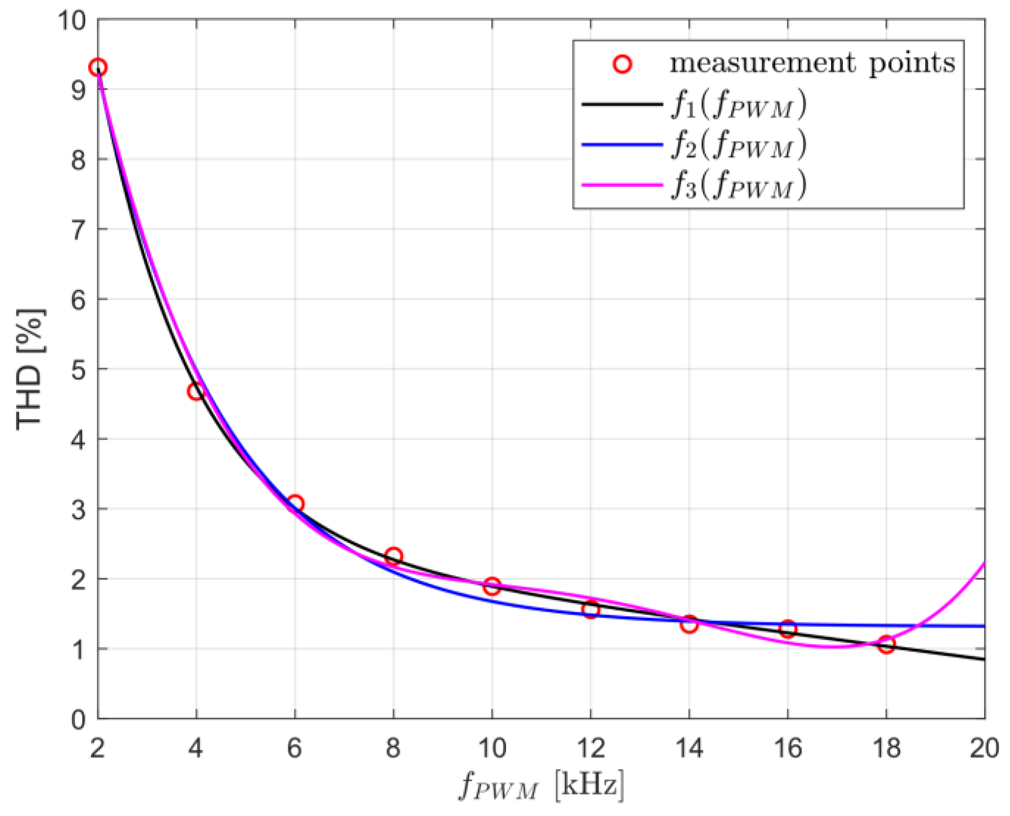
where x (in Matlab) denotes the parameters of the $\alpha$ of Equation (9). If we measure THD of current for different values of switching frequencies of VSI transistors, for example, every f_PWM = 2 kHz, then it is possible to make an approximation of THD changes from f_PWM (THD = f(f_PWM)). The accuracy of the approximation depends on the function adopted. Figure 1 shows the approximation of measurement points by three different functions:

$$f_1\left(f_{PWM}\right)=a_1+a_2{e}^{a_3{f}_{PWM}}+a_4{f}_{PWM},$$

(10)

$$f_2\left(f_{PWM}\right)=a_1+a_2{e}^{a_3{f}_{PWM}},$$

(11)

$$f_3\left(f_{PWM}\right)=a_1+a_2{f}_{PWM}+a_3{f}_{PWM}^2+a_4{f}_{PWM}^3+a_5{f}_{PWM}^4$$

(12)

The values of resnorm (from the lsqcurvefit function) or J are as follows for each function: $J_1=0.0244, J_2=0.2787, J_3=0.1938$. These values mean that the best fit to the measurement points is for function $f_1$, which differs from $f_2$ only by a linear factor. Increasing the order of the polynomial in function $f_3$ makes no sense because it leads to interpolation, thus no longer averaging the results. This example precedes the rest of the study, but it is the f_1 function that will be used in the approximation of THD changes from $f_{PWM}$.

3. VSI with SVPWM Control

Nowadays, voltage modulation of the SVPWM inverter is the most popular; the hardware is based on a timer with 3 values for comparison. The result is 3. rectangular waves that control the inverter transistors. Due to the longer transistor turn-off time than turn-on time, a turn-on-dead band (dead time) delay is used. In the following, SVPWM methods and the effects of dead bands will be discussed and compared in the simulation section.

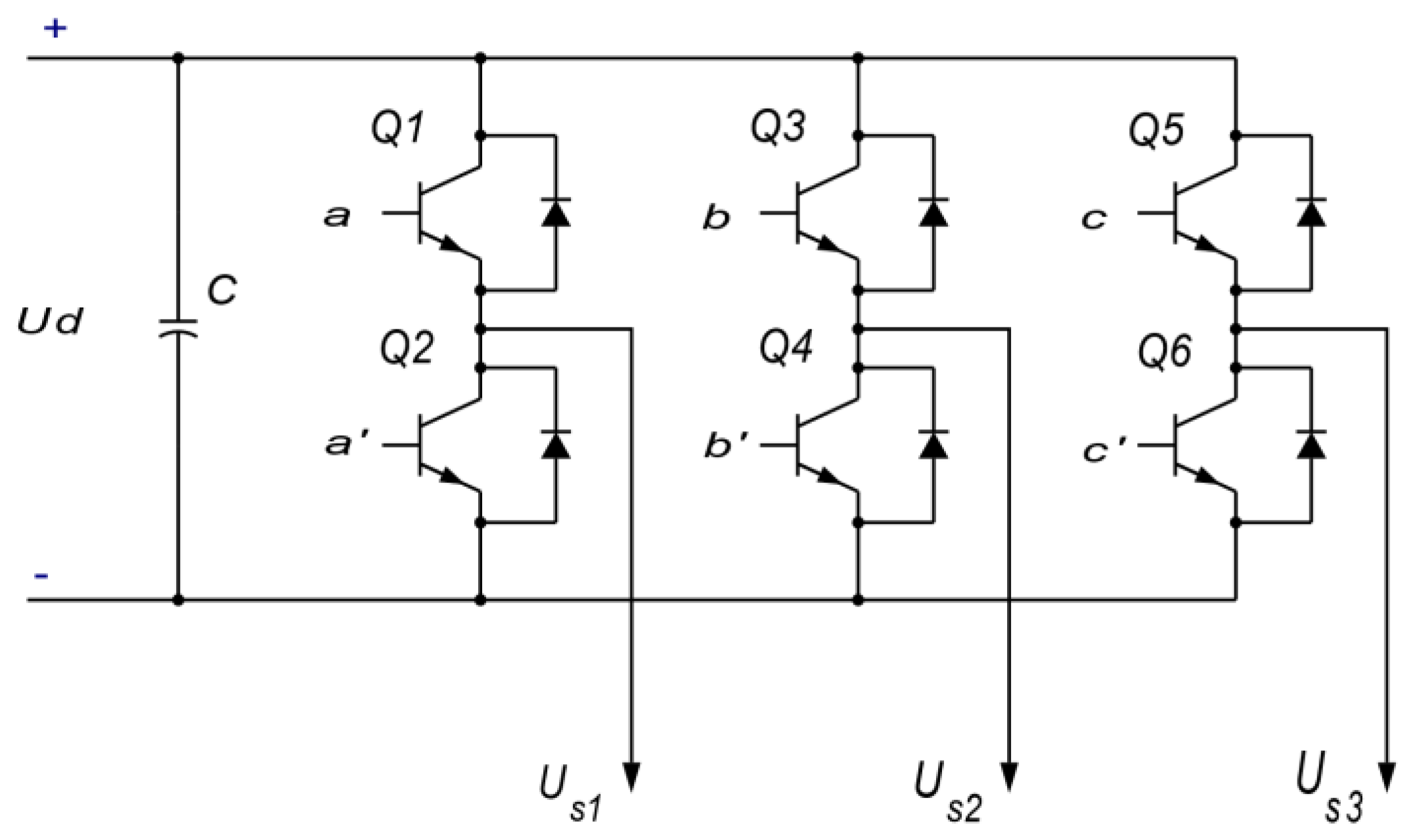
The Voltage Source Inverter is shown in Figure 2, where the logic signals (a,a′), (b,b′), and (c,c′) are complementary, i.e., if a = 1, then a′ = 0, and so on. In addition, there is a delay between turning off the transistor and turning it on—dead band.

The controls a, a′, b, b′, c, and c′ are assumed to be logical (0, 1), while U_S1, U_S2, and U_S3 are the motor phase voltages. It follows that there are eight possible control settings (a, b, c) that determine the switching sequence of the power transistors (Q1 ÷ Q6).

The transistors are controlled by PWM signals of appropriate fills with the appropriate switching frequency $f_{PWM}$ which leads to the generation of three-phase average (in small time) sinusoidal voltage waveforms.

3.1. The Method

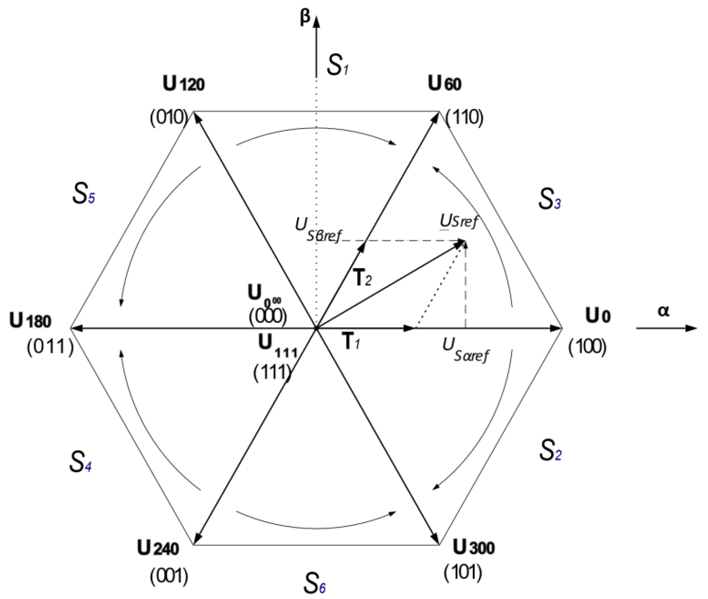
The method is based on controlling six transistors in the three-phase bridge voltage inverter circuit shown in Figure 2. In such a system, the different states of the control inputs (a, b, c), together with the PWM space vector (SVPWM), form a hexagon of output voltages with an additional two null controls (${\mathrm{U}}_{000},{ \mathrm{U}}_{111}$). These eight vectors are called base space vectors:${ \mathrm{U}}_0$, ${\mathrm{U}}_{60}$, ${\mathrm{U}}_{120}$, ${\mathrm{U}}_{180}$, ${\mathrm{U}}_{240}$, ${\mathrm{U}}_{300}$,${\mathrm{U}}_{000},{ \mathrm{U}}_{111}$. The geometric interpretation of the voltage space vectors is shown in Figure 3.

The reference voltage ${\underset{\_}{U}}_{Sref}$ represents the interfacial mean value in the (α, β) coordinate system:

$$\frac{1}{T_{PWM}}{{\displaystyle \int }}_0^{T_{PWM}}{\underset{\_}{U}}_{Sref})t_{dt}=\frac{1}{T_{PWM}}(T_1{\underset{\_}{U}}_x+T_2{\underset{\_}{U}}_{x\pm 60}),$$

(13)

where T₁ and T₂ are the individual turn-on times of the given base vectors $U_x$ and $U_{x\pm 60}$, and $T_{PWM}$ is the period of PWM signal generation. When $\left|{\underset{\_}{U}}_{Sref}\right|<U_d$, then in addition to T₁ and T₂ times, modulation requires the supply of the vectors $U_{000}$ or $U_{111}$ at time T₀. Then:

$$T_1+T_2+T_0=T_{PWM}.$$

(14)

Various relationships can be used to determine T₁ and T₂ times (3)–(7) and the results obtained are identical. There are two SVPWM methods, referred to as Pattern #1 (Three-phase SVM with Symmetrical Placement of Zero Vectors) and Pattern #2 (Two-phase SVM). This type of modulation is called discontinuous pulse width modulation (DPWM) (3) and (8). These modulation methods differ in the generation times of zero-voltage vectors with a duration of T₀.

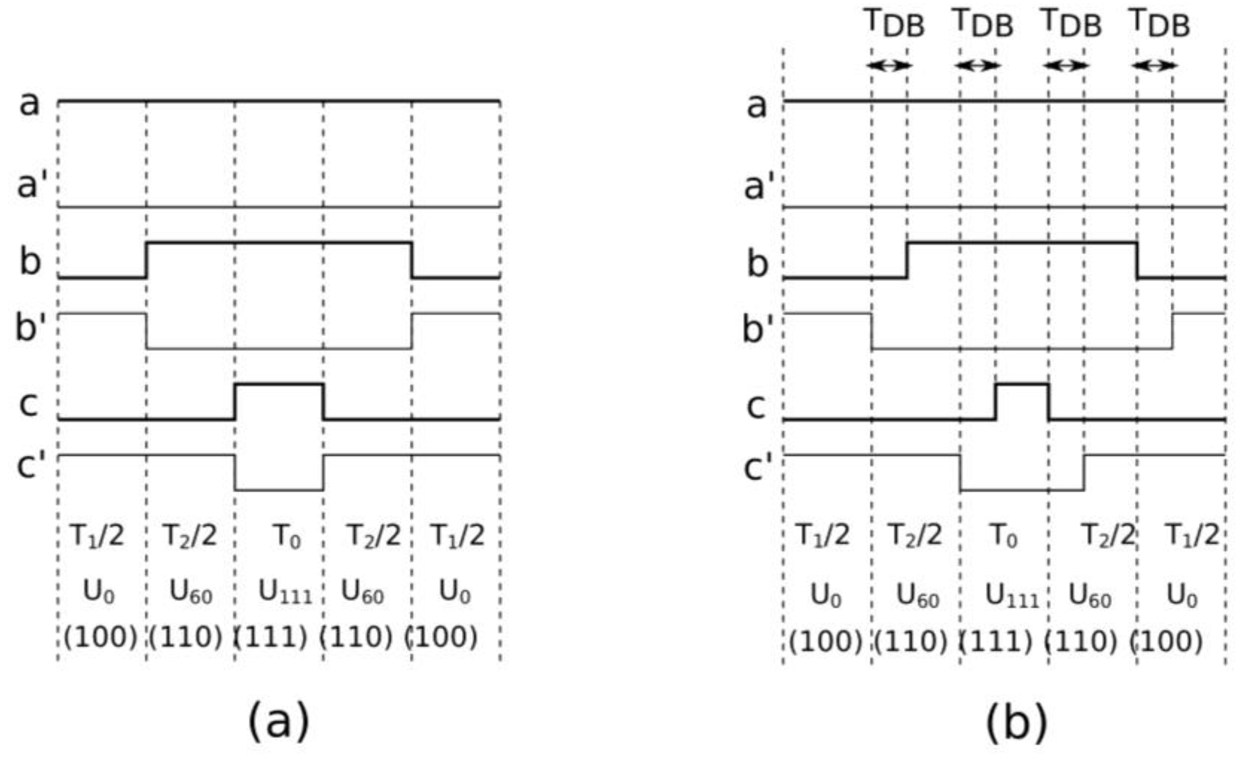
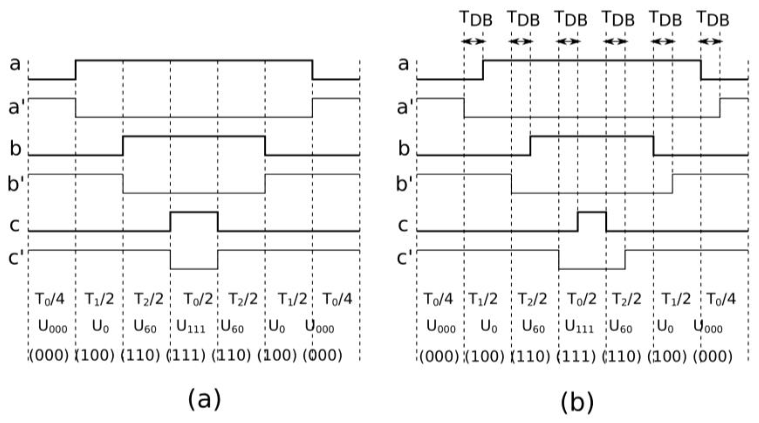
3.2. Switching Pattern #1

The SVPWM with switching Pattern #1 is the most popular SVM method. An example of transistor control for this method and sector from 0° to 60° is shown in the Figure 4. Presented here is the ideal case and applications of dead times T_DB when transistors in one branch are switched.

Usually, dead time is small and a few μs, but it will still affect the voltage waveform distortion and, therefore, the motor current waveform distortion. Quantitative results will be presented in the chapter on simulation studies.

3.3. Switching Pattern #2 (DPWM)

In Pattern #2, there is less symmetry of PWM waveforms; the T0 time of zero voltage generation is not divided into three intervals, but is generated once. An example for the first sector is presented in Figure 5.

In this modulation method, the number of transistor switching is reduced by one-third, but at the same time, due to the asymmetry of the waveforms, the harmonic content (THD) is increased. Note also that the amount of $T_{DB}$ generation also decreases by one-third compared to the Pattern #1 method. Therefore, it is interesting to see how THD will change as the switching frequency of $f_{PWM}$ transistors increases. These results will be presented in the next section.

4. Induction Motor Model

The mathematical model of the induction motor is well known from the literature [1,2,3,4,5,6,7,8,9], so it will be presented briefly, using only the most important equations. It will be reduced to the classical form of Rotor Field-Oriented Control (RFOC), which will be used in the analysis of the power supply from the SVPWM modulator.

Vector analysis and synthesis of induction motor drives use transformations to the $\alpha , \beta$ and d-q system (subscript s applies to phase currents 1,2,3) [1,2,3,4,5,6,7,8,9,10,11,12]:

$$\{\begin{array}{ll}{i}_{S\alpha }\left(t\right)\hfill & = i_{S1}\left(t\right)\hfill \\ i_{S\beta }\left(t\right)\hfill & = \frac{\sqrt{3}}{3}\left[i_{S2}\left(t\right)-i_{S3}\left(t\right)\right]\hfill \end{array}$$

(15)

$$\{\begin{array}{c}{i}_{Sd}=i_{S\alpha }\cos {\varrho }_R+i_{S\beta }\sin {\varrho }_R\\ i_{Sq}=-i_{S\alpha }\sin {\varrho }_R+i_{S\beta }\cos {\varrho }_R\end{array}$$

(16)

where ${\varrho }_R$ is the angle of alignment of the coordinate system (d-q), which is aligned with the position of the vector of rotor linked flux ${\underset{\_}{\psi }}_R$ (where ${\varrho }_R$ is the angle between the stator axis and the rotor flux vector). After assuming such a reference system, it can be written [1,2,3,4,5,6,7,8,9] (where $L_R, L_{\mu }$ are rotor and magnetizing inductances; the vector ${\underset{\_}{i}}_R, {\underset{\_}{i}}_S {\underset{\_}{i}}_{mR}$ are rotor, stator, and magnetizing currents):

$${\underset{\_}{\psi }}_R=L_R{\underset{\_}{i}}_R+L_{\mu }{\underset{\_}{i}}_S=L_{\mu }{\underset{\_}{i}}_{mR}, {\underset{\_}{i}}_{mR}=\frac{{\underset{\_}{\psi }}_R}{L_{\mu }}=\frac{L_R}{L_{\mu }}{\underset{\_}{i}}_R+{\underset{\_}{i}}_S$$

(17)

thus,

$${\underset{\_}{\psi }}_R=\left|{\underset{\_}{\psi }}_R\left|={\psi }_R=L_{\mu }\right|{\underset{\_}{i}}_{mR}\right|=L_{\mu }{i}_{mR},$$

(18)

and the coordinate system (d-q) is rotating at a speed ${\omega }_{mR}=\frac{d{\varrho }_R}{dt}$.

The final mathematical model when decomposed into d-q components takes the following form:

$$T_R\frac{d{i}_{mR}}{dt}+i_{mR}=i_{Sd}$$

(19)

$${\omega }_{mR}=\frac{d{\varrho }_R}{dt}=p_b{\omega }_m+\frac{i_{Sq}}{T_R{i}_{mR}}=p_b{\omega }_m+{\omega }_2$$

(20)

where ${\omega }_2$ pulsation (speed) of slip, and $T_R=\frac{L_R}{R_R}$ ($L_R,R_R$ are inductace and resistace of rotor circuit) is rotor electromagnetic time constant. The voltage equations are in the form:

$$u_{Sd}=R_S{i}_{Sd}+\left(1-\sigma \right)L_S\frac{d{i}_{mR}}{dt}+\sigma L_S\left(\frac{d{i}_{Sd}}{dt}-i_{Sq}{\omega }_{mR}\right)$$

(21)

$$u_{Sq}=R_S{i}_{Sq}+\left(1-\sigma \right)L_S{i}_{mR}{\omega }_{mR}+\sigma L_S\left(\frac{d{i}_{Sq}}{dt}+i_{Sd}{\omega }_{mR}\right)$$

(22)

where $R_S, L_S$ are are the resistance and inductance of rotor; $\sigma$ is leakage factor.

The model is summarized by the equation of motion (Newton’s second principle of dynamics):

$$J\frac{d{\omega }_m}{dt}=\stackrel{M_e}{\overbrace{\underset{K}{\underbrace{\frac{3}{2}{p}_b\left(1-\sigma \right)L_S}}{i}_{mR}{i}_{Sq}}}-M_m$$

(23)

The above equations are a system of nonlinear differential equations that are difficult to analyze, and practically only numerical methods can be used here to precisely determine the operating conditions of the induction motor.

5. Simulations and Approximation

In the article, steady-state waveforms are studied because THD can then be determined. For this reason, motor startup (transient) was not studied and was only needed to obtain steady-state operation of the machine.

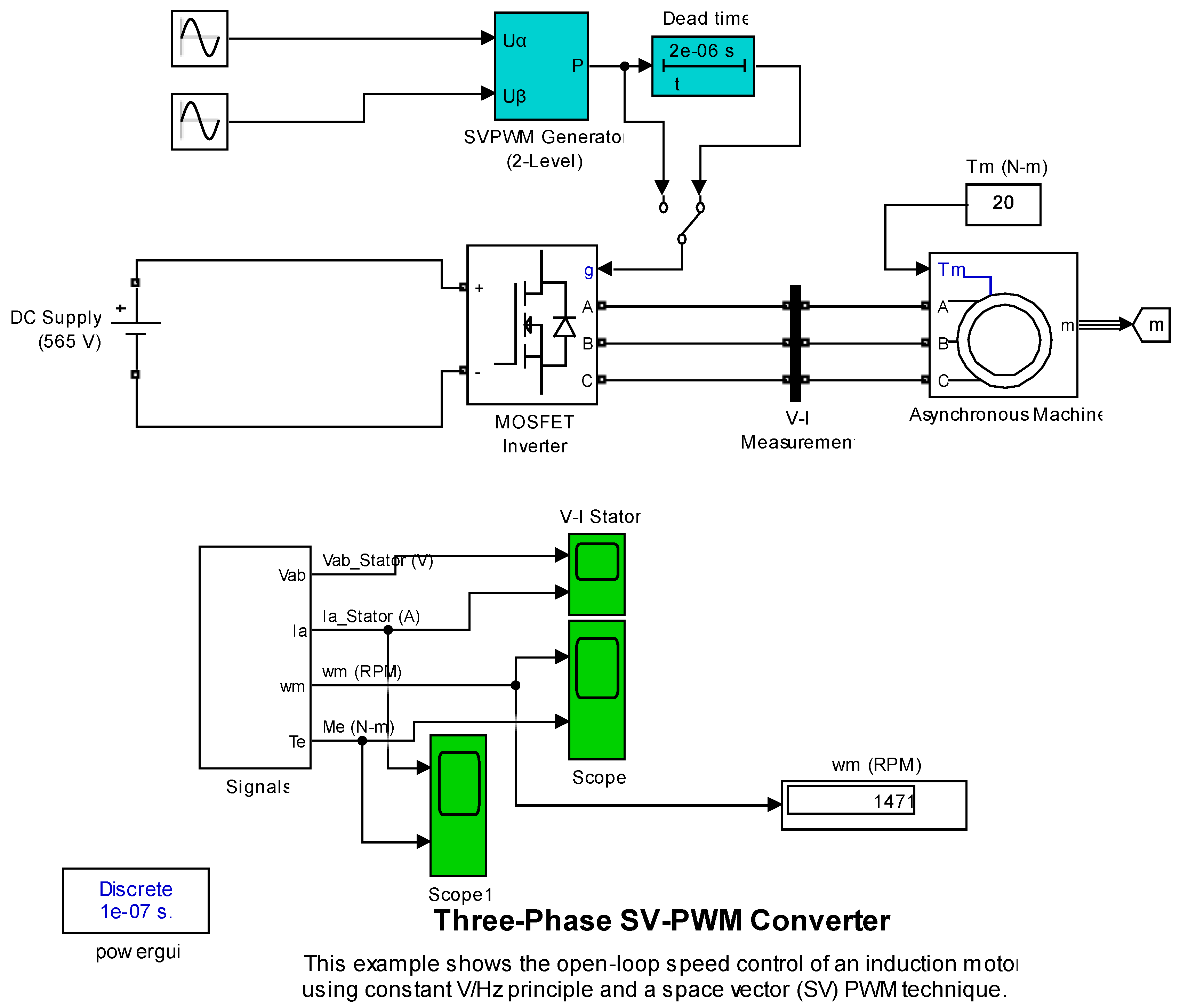
The simulation research used the standard simulation power_svpwm.slx (Matlab 2020b), which is supplemented with the dead time (dead band) block from the simulation power_microturbineDT.slx is shown in Figure 6.

The simulation diagram is composed of two standard diagrams, so anyone can repeat the tests, which are included below. Only the generators of the alpha and beta components of the stator voltage need to be added, and the alpha-beta components (data type of input reference vector (Uref)) should be set in the SVPWM Generator block. The powergui block is used to configure the simulation and THD determination, with the integration time and differential equations integration method displayed in blue.

Squirrel-cage preset model no 2 from Asynchronous Machine menu is used: 7.46 kW, U_N = 460 Vrms, pole pairs = 2. This is a standard model and does not take into account saturation in steel. SVPWM Generator allows you to select the modulation method: Pattern #1 or Pattern #2; in addition you can select PWM frequency and sample time. Dead time block should have selected type: on delay and time delay as time value in seconds. In the research, the setting was 1 μs or 2 μs.

All tests were conducted for a motor start connected to a power supply with a fixed Us and f1, where f1 is the power supply frequency of 50 Hz. Results were obtained for steady-state operation.

In the simulation study, a smaller than rated value of the load torque was assumed, which is 20 Nm instead of 40.5 Nm (rated value). There are three reasons for this determination of simulation conditions:

• A smaller current leads to a larger THD and larger ripples of the electromagnetic torque. For this reason, it is easier to determine the shape of the steady-state characteristics;
• Simulation time is proportionally shorter: the simulations were performed on a Lenovo X1 laptop (Intel i7-8650U, 16 GB RAM) and lasted more than 4′;
• Electric motors can operate with different load torques and in continuous operation in the 0–$M_N$ range. Below $M_N$, both THD and electromagnetic torque ripple are greater than the rated conditions.

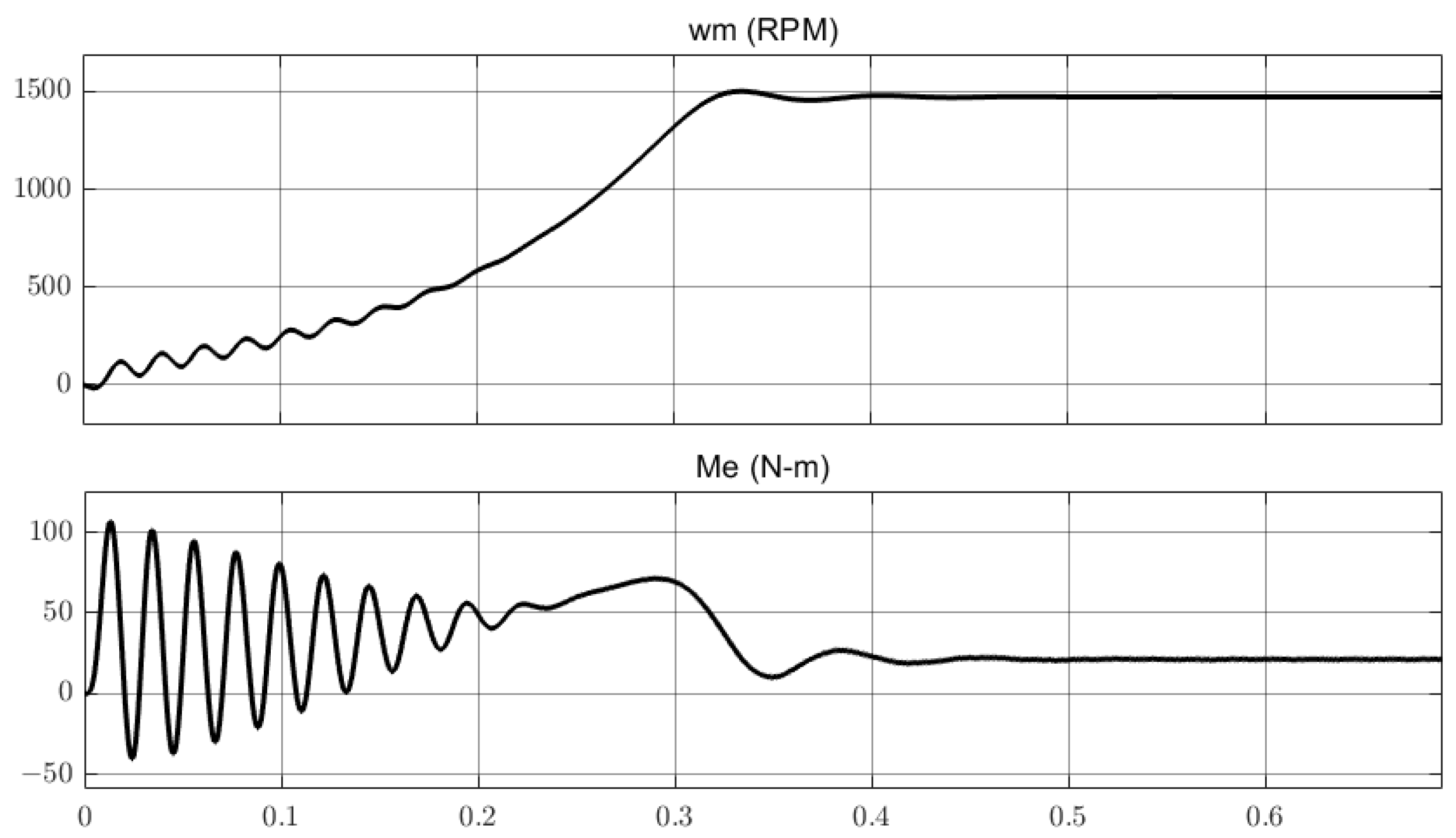
An example induction motor startup for a transistor switching frequency of $f_{PWM}=6 \mathrm{kHz}$ and dead time of 0 μs is shown in Figure 7. This is one simulation out of 54, the results of which will be analyzed below.

When the supply voltage is applied to the motor’s stator windings, torque oscillations occur, which are transferred to angular velocity oscillations. The reason for the oscillations is the design of the induction motor, which is described by a nonlinear mathematical model where two circuits are coupled to each other, Equations (21) and (22). A detailed description of the phenomena is presented in sub-Section 5.2.

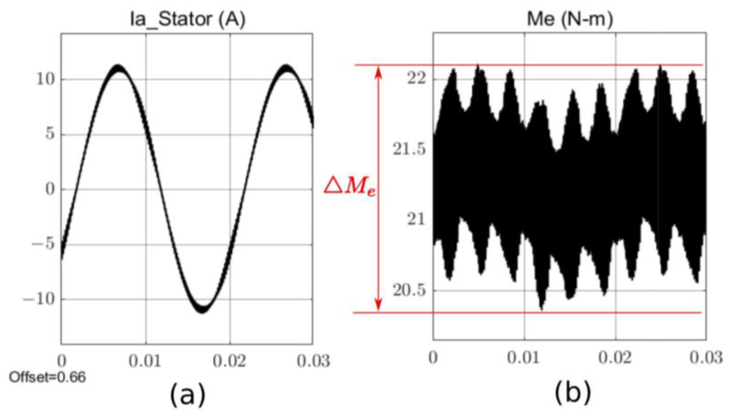
The steady-state current $i_{S1}$ and electromagnetic torque $M_e$ are shown in Figure 8. Using such measurements, Figure 8 presents the resulting effect of $f_{PWM}$ frequency on THD and torque ripple ($\Delta M_e$).

The experiment was conducted for different VSI switching frequencies (f_PWM), different control strategies Pattern #1 and Pattern #2, and different dead times (dead band). The results of the experiment are current THD and IM electromagnetic moment ripple. The amplitude of changes in the electromagnetic torque (torque ripple) was determined from the Me waveform as shown in Figure 8. Determining the maximum and minimum values from the presented waveform introduces reading errors, but the approximation has the property of averaging the results (it will be shown in the next part of the paper). Therefore, approximation use is justified.

The obtained results are summarized in

Table 1. Comparison THD and torque ripple for different PWM frequency, different dead band, different modulation pattern.

FPWM [kHz]	${\mathit{T}}_{\mathit{D}\mathit{B}} \left[\mathsf{\mu }\mathbf{s}\right]$	THD		$\mathbf{\Delta }{\mathit{M}}_{\mathit{e}} \left[\mathbf{Nm}\right]$
		Pattern #1	Pattern #2	Pattern #1	Pattern #2
2	0	9.31%	10.77%	4.1	5.2
2	1	9.24%	10.72%	4.1	5.3
2	2	9.19%	10.73%	4.2	5.4
4	0	4.63%	5.35%	2.1	3.95
4	1	4.58%	5.36%	2.15	3.9
4	2	4.57%	5.36%	2.2	3.9
6	0	3.07%	3.55%	1.45	2.55
6	1	3.05%	3.57%	1.63	2.65
6	2	3.17%	3.59%	1.65	2.8
8	0	2.32%	2.66%	1.1	2.05
8	1	2.42%	2.70%	1.59	2.1
8	2	2.79%	2.79%	1.53	2.25
10	0	1.89%	2.16%	0.95	1.79
10	1	2.20%	2.30%	1.32	1.66
10	2	2.88%	2.50%	1.76	1.88
12	0	1.56%	1.80%	1.03	1.42
12	1	1.88%	1.93%	1.57	1.41
12	2	2.86%	2.22%	1.41	1.63
14	0	1.35%	1.57%	0.9	1.15
14	1	2.01%	1.78%	1.09	1.21
14	2	3.29%	2.30%	1.4	1.45
16	0	1.28%	1.36%	0.7	0.65
16	1	2.10%	1.57%	1.11	1.15
16	2	3.52%	2.23%	1.48	1.45
18	0	1.06%	1.23%	0.78	0.99
18	1	2.17%	1.58%	1.17	1.08
18	2	3.78%	2.35%	1.62	1.49

. Simulations were carried out by setting the solver as fixed-step and the integration step to 1 × 10⁻⁷. For the shortest dead time, i.e., 1 μs, 10 samples per delay time are obtained, according to the sampling theorem. Experiments were realized with smaller integration times, but because the results did not differ, the previously given one was stayed. The choice of such a time can be commented on in another way: if we want to observe the effect of delays at the 1 μs level, then the integration time of the numerical method must be much smaller. Fixed step guarantees equal time distances between samples (fixed sampling frequency), so the spectrum is calculated precisely.

5.1. Approximation of Current THD

An approximation of the measurement data for the various cases in Table 1 was performed, grouped together, and shows the following:

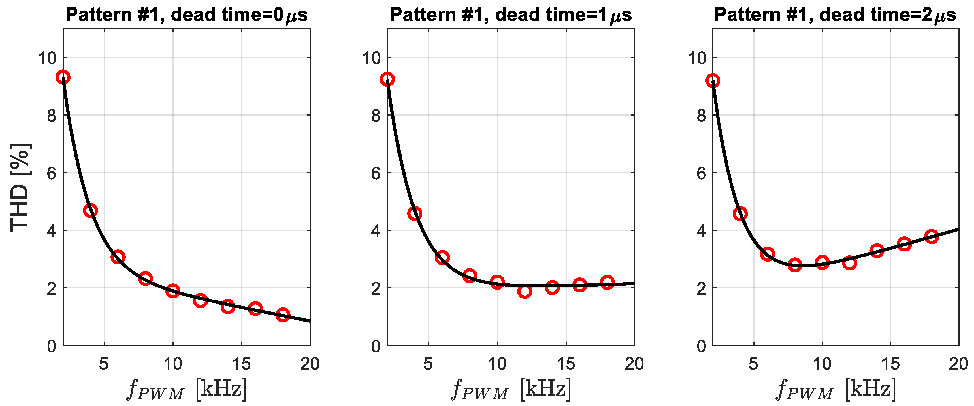
• Figure 9—change of THD for Pattern #1 at different dead time T_DB = 0, 1, 2 us;
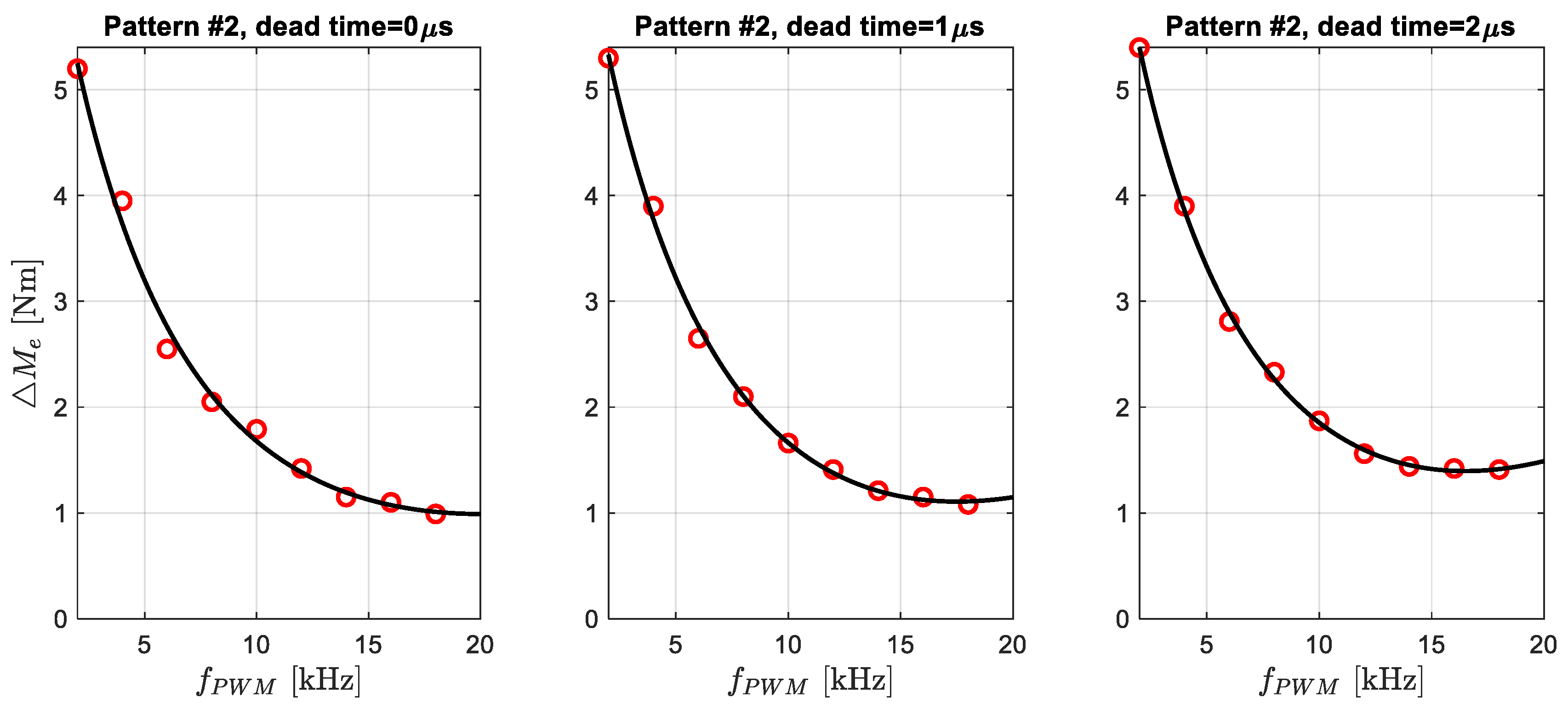
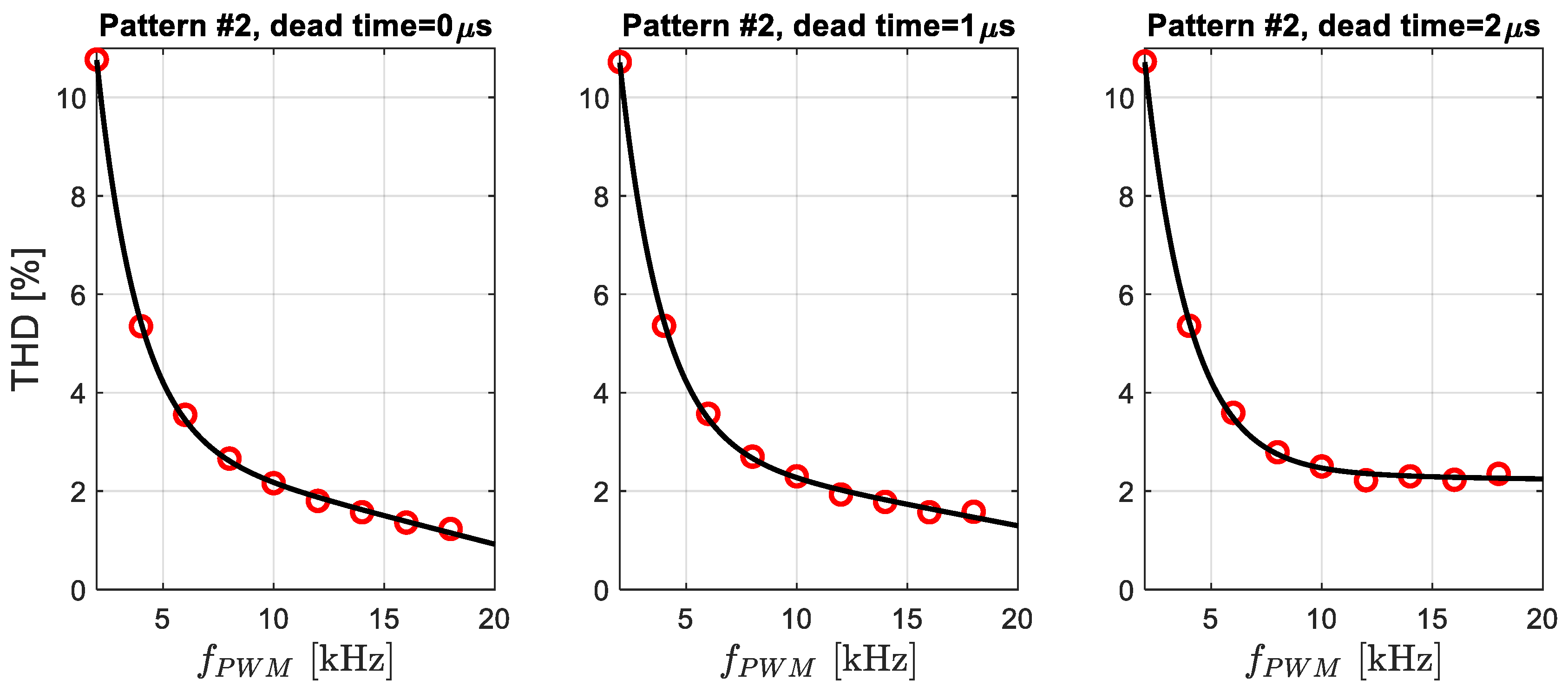
• Figure 10—change of THD for Pattern #2 at different dead time T_DB = 0, 1, 2 us;

The results are presented by applying titles to each figure, rather than (a), (b), (c), so the results are more readable.

The first graphs in the figures show THD changes for ideal inverter control, that is, for perfect transistors (T_DB = 0 us). They appear only for comparison with the other cases.

Analyzing the obtained results, it can be seen that switching frequencies of transistors $f_{PWM}$ lower than 6 kHz should not be used. Below this frequency, THD is less than 4; that is, approximately the current waveform deviates from the sinusoid by about 4%. This is usually an acceptable value for induction motors.

The approximation function was (10). Comparing the characteristics in Figure 9 and Figure 10, the following effect of dead time on the switching of inverter transistors can be observed:

• T_DB = 0 us, then modulation Pattern #1 has better characteristics than Pattern #2. This is the ideal case, and this result is obvious;
• T_DB = 1 us, up to 10 kHz better THD is obtained for Pattern #1 modulation, but above 10 kHz. Pattern #2 modulation has better THD;
• T_DB = 2 us, up to 8 kHz SV-PWM with switching Pattern #1 obtains better results than for Pattern #2, while for higher switching frequencies of transistors the situation is reversed, and a large value of dead time negatively affects the implementation of switching Pattern #1. This is due to the higher number of transistors switching to generate the voltage $U_{sref}$.

Summarizing the results obtained and looking only through the spectrum of currents (THD), it can be concluded that up to a PWM frequency of 8 kHz, it is best to use Pattern #1 modulation, while above 8 kHz it is best to use Pattern #2 modulation. These results will be confirmed with torque ripple analysis.

5.2. Torque Ripples Approximation

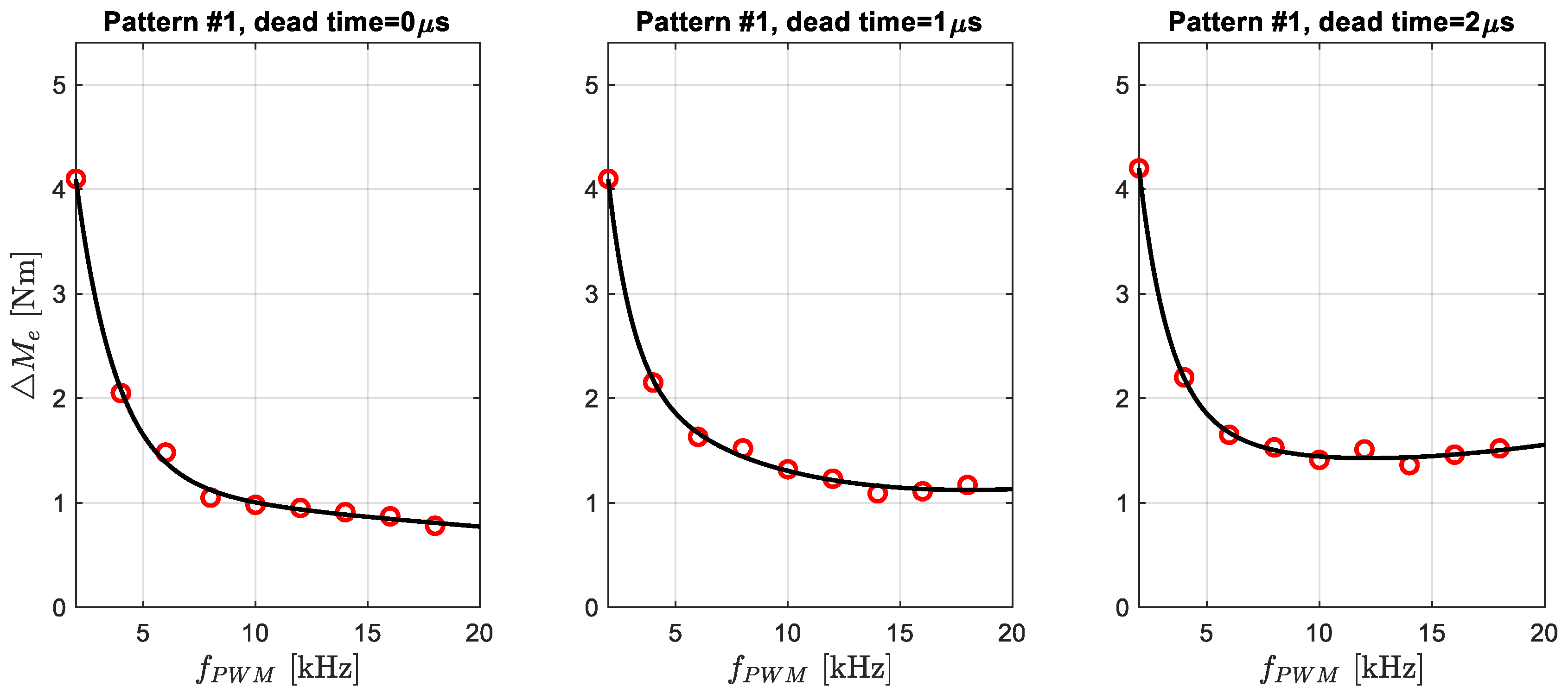
The next results were obtained for the estimation of the electromagnetic torque ripples $\Delta M_e$ and are shown in the following figures, respectively, for Pattern #1 (Figure 11) and Pattern #2 (Figure 12). After many trials, a function with six coefficients was chosen as the best function to approximate the obtained results:

$$f_4\left(f_{PWM}\right)=a_1+a_{2}x+a_4{e}^{a_{4}x}+a_5 x^{a_6}$$

(24)

Torque ripples $\Delta M_e$ were estimated as shown in Figure 11, i.e., the accuracy of the data presented is approximate. For this reason, the use of the approximating function (10) here is most advisable, and it will average out the measurement errors.

A quick comparison of simulation results after approximation leads to the following conclusion: for switching Pattern #1, moment ripples below 2% are obtained for f_PWM = 6 kHz, and for switching Pattern #2 for 10 kHz, 2% was chosen as a value already satisfactory to the $\Delta M_e$. This is not the final conclusion, however, and a more detailed analysis of the obtained results should be made.

The analysis of electromagnetic torque ripple is not as obvious as for current THD. A different approximating function was used here because the measurement points are arranged differently. In addition, no significant rise in the characteristic for switching Pattern #1 in the higher frequency range can be seen here. Above 10 kHz, the compared characteristics (for Pattern #1 and #2) differ by less than 0.5 Nm. As the frequency increases, these differences decrease, and for 16 kHz and 18 kHz, they are already practically indistinguishable.

To analyze the changes in $\Delta M_e\left(f_{PWM}\right)$, it is necessary to return to the induction motor model (Section 4). The inverter powers the motor, not the RL circuit, which means that in addition to currents, voltages, and linked fluxes, there is an electromagnetic torque and back electromotive forces.

The ordinary differential equations of an induction motor are nonlinear, which is especially evident in the voltage Equations (21) and (22). The electromagnetic torque is generated according to relation (23) and is the product of two currents $i_{mR}$ and $i_{Sq}$. The q-axis current is determined directly from the geometric transformation (16), and the $i_{mR}$ current is the result of filtering (19). When the motor is fed with signals such as those in Figure 4 and Figure 5, it is impossible to speak of steady state. In addition, in Equations (21) and (22), you can see the phenomenon of coupling between the two circuits (in the d and q axis); i.e., the current $i_{mR}$ is produced by the voltage $u_{Sd}$ but affects the current $i_{Sq}$ (expression $\left(1-\sigma \right)L_S{i}_{mR}{\omega }_{mR}$ in (22)).

In addition, the current $i_{Sd}$ also affects the current $i_{Sq}$ (expression $\sigma L_S{i}_{Sd}{\omega }_{mR}$). In the other direction, coupling also occurs; i.e., current $i_{Sq}$ is produced by voltage $u_{Sq}$ and affects currents $i_{Sd}$ and $i_{mR}$ (expression $-\sigma L_S{i}_{Sq}{\omega }_{mR}$ in (21)). Hence, the induction motor is a strongly nonlinear system and with SVPWM control there is a permanently dynamic state, which we can only determine using numerical methods. The effect of circuit coupling is analytically impossible changes in $\Delta M_e\left(f_{PWM}\right)$, which are different from THD($f_{PWM}$).

6. Experiments

Simulation results showed the similarity of the current THD and torque ripple $\Delta M_e$. For this reason, experimental research was presented for THD current analysis. Additionally, the lab stand shown below does not have a torque sensor, so measuring $\Delta M_e$ is impossible.

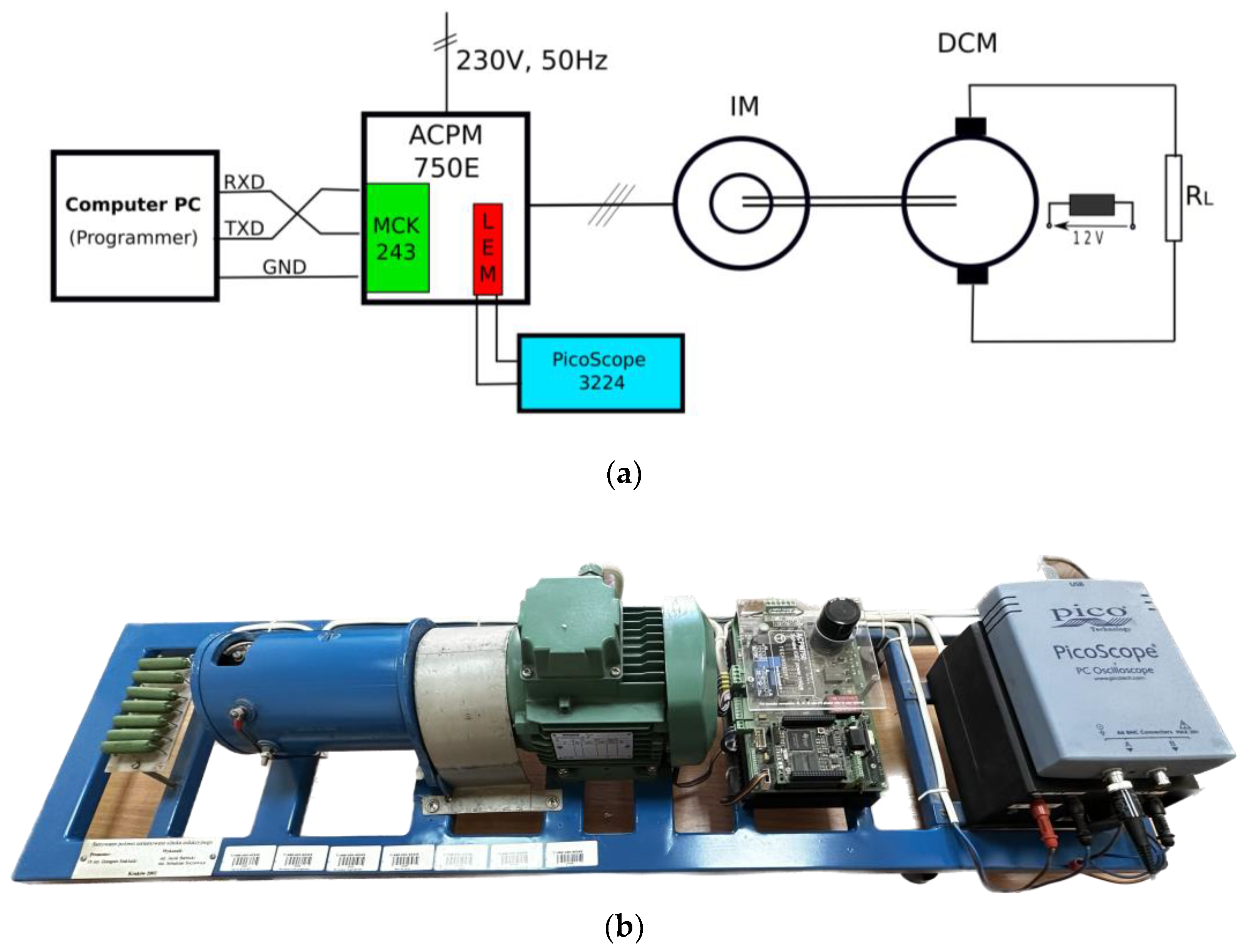
6.1. Experimental Setup

The experimental setup is shown in Figure 13, where Technosoft’s DMCS-as software (version 1.3) installed on a PC was used.

The squirrel cage induction motor IM (350 W, 2850 rpm, number of pole pairs = 1) is loaded with a DCM generator, where the load torque is varied by the excitation current. The ACPM 750E and MCK243 are also Technosoft products and are respectively a VSI (750 W) and a control circuit with a TMS320F243 processor. The control circuit generates PWM signals for the inverter transistors according to Pattern #1, where the switching frequency and dead band can be changed. For this reason, experimental results for Pattern #2 are not included, but confirmation of simulation results is expected.

Comparing the simulation scheme in Figure 6 and the experimental setup in Figure 13 reveals the following:

• SVPWM Generator and dead time (Figure 6) are implemented by the TMS320F243 processor located in the MCK243 module (Motor Control Kit), which is connected to the ACPM 750E;
• The TMS320F243 processor is 16 bit and has a 20 MHz clock; the timer for SVPWM implementation is also 16 bit. The importance of the frequency of counted pulses in PWM is explained in sub-Section 6.4;
• MOSFET inverter and block signals (current and voltage measurement) in Figure 6 is part of the ACPM 750E, where LEM current transducers are placed;
• Scope V-I Stator (visualization) is realized in practice by PicoScope;
• In the experimental setup, a DCM generator was used as the load, and in Figure 6 is the constant block. The analysis of current signals is realized for steady state, so such a torque setting as in Figure 13 is sufficient.

The LEM (stator current measurement) transducer is located on the ACPM board, and the current waveform can be recorded. The PicoScope3224 is used for this purpose. PicoScope 3224 is the USB PC Oscilloscopes with data logger. This model is the two-channel version and has the following features:

• 20 MS/s maximum sampling rate;
• 512,000 sample buffer;
• 12-bit resolution;
• USB 2.0 interface;
• ±20 mV to ±20 V measuring ranges;
• 10 MHz analogue bandwidth and spectrum analyzer range.

The 12-bit resolution allows the THD to be accurately determined for 3128 samples per period leading to a sampling frequency of 156.4 kHz). Such is the value set in the PicoScope 7 (version 7.0.116.13984) control software.

6.2. Measurement Results

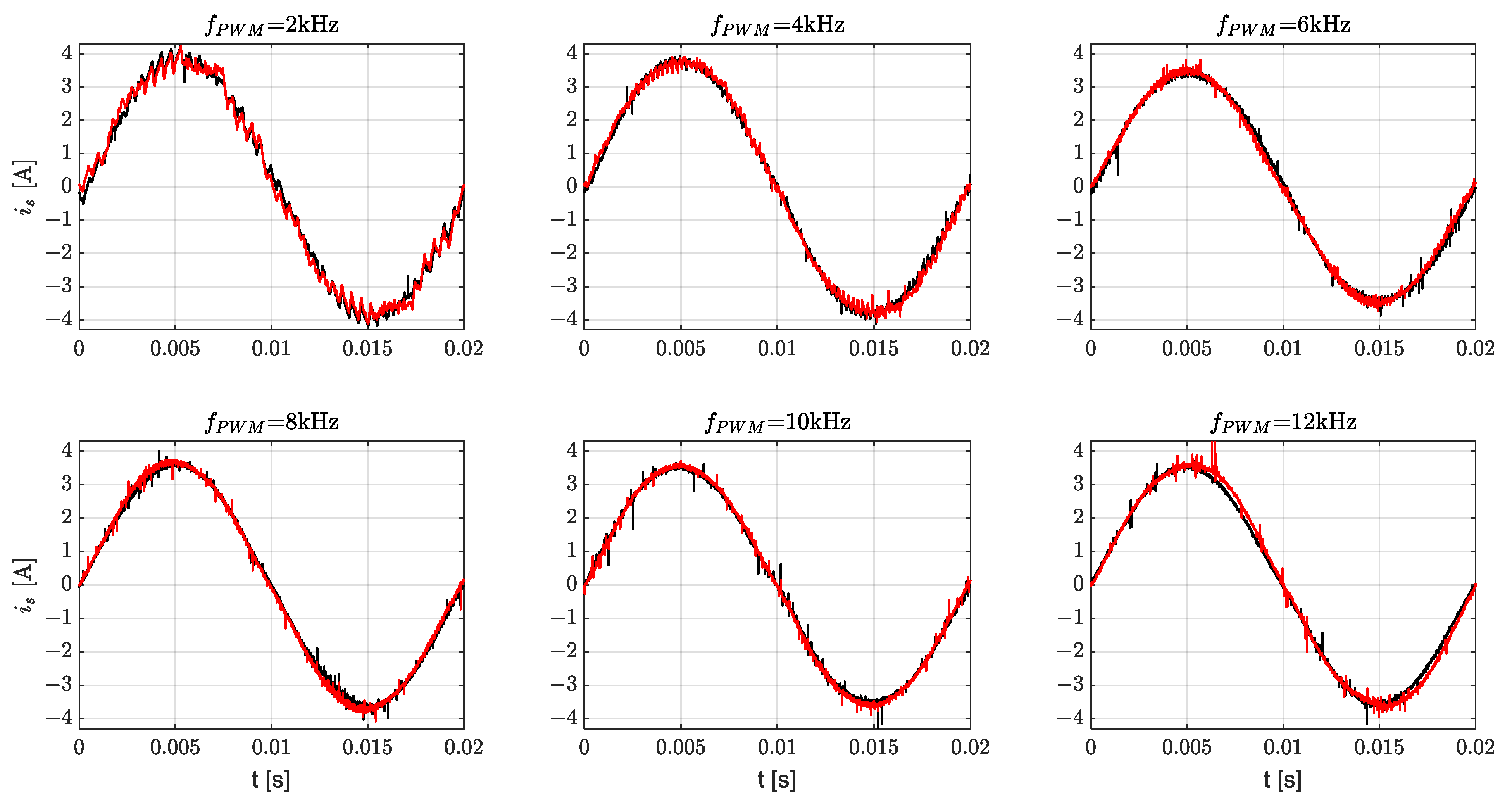
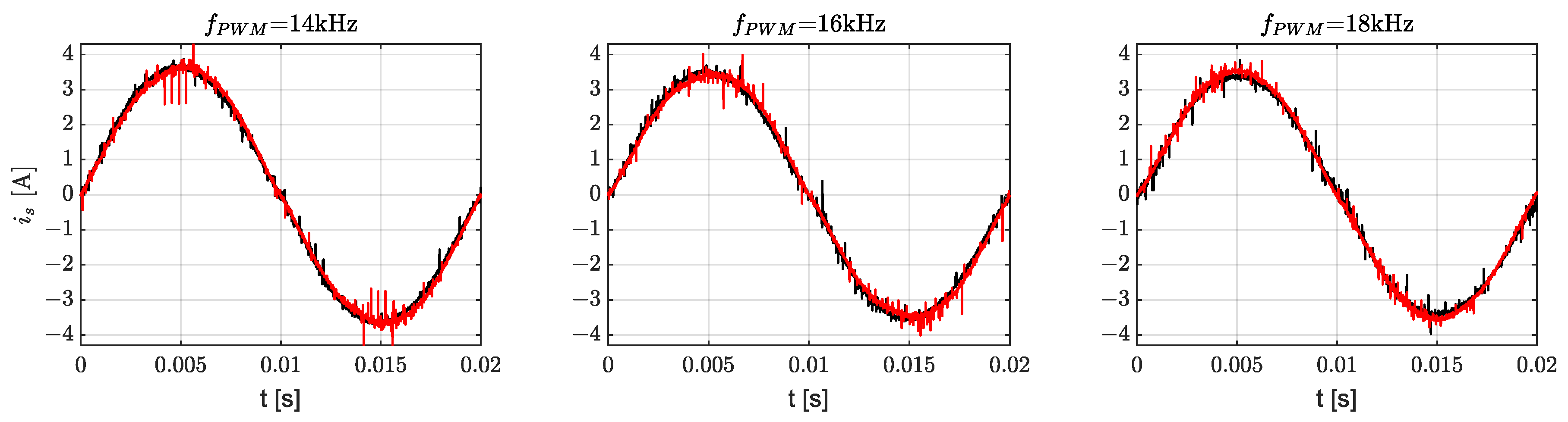
The results of the experiments are shown in Figure 14 and Figure 15, where the current waveforms for PWM modulation with Pattern #1 and different dead times $T_{DB}$ are compared. The following figures show comparisons for different switching frequencies of $f_{PWM}$, as indicated in their titles.

Figure 14 and Figure 15 show the raw results of the measurements, i.e., no signal filtering was applied. Therefore, you can clearly see the measurement noise here, which is random and will not affect the result of the FFT and therefore the THD.

6.3. THD Analysis

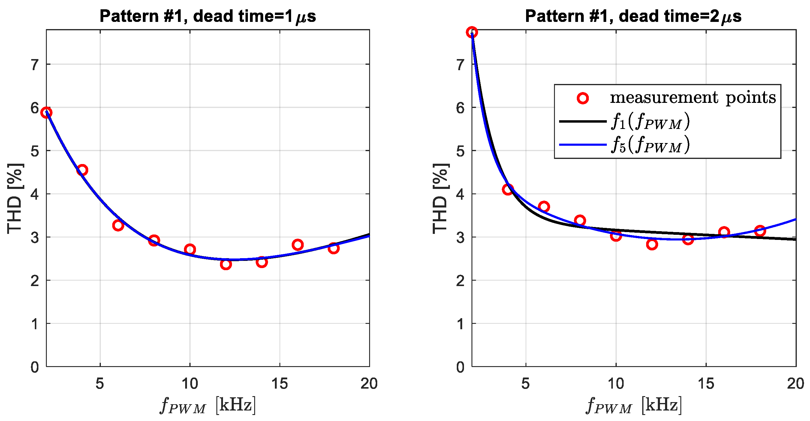
The results of the measurements are presented in

Table 2. Comparison THD for different PWM frequency, different dead band for pattern #1.

fPWM [kHz]	$\mathrm{THD}$		$\mathit{\gamma }$ [%]
	${\mathit{T}}_{\mathit{D}\mathit{B}}=1 \mathsf{\mu }\mathbf{s}$	${\mathit{T}}_{\mathit{D}\mathit{B}}=2 \mathsf{\mu }\mathbf{s}$	${\mathit{T}}_{\mathit{D}\mathit{B}}=1 \mathsf{\mu }\mathbf{s}$	${\mathit{T}}_{\mathit{D}\mathit{B}}=2 \mathsf{\mu }\mathbf{s}$
2	5.88%	7.74%	0.4	0.8
4	4.55%	4.11%	0.8	1.6
6	3.27%	3.70%	1.2	2.4
8	2.92%	3.38%	1.6	3.2
10	2.71%	3.03%	2.0	4.0
12	2.37%	2.83%	2.4	4.8
14	2.42%	2.95%	2.8	5.6
16	2.82%	3.11%	3.2	6.4
18	2.74%	3.14%	3.6	7.2

and Figure 16, which shows a comparison of THD for selected PWM frequencies and dead time (Pattern #1 modulation method). The tests were performed at the same frequencies as in the simulation studies. To describe the effect of dead band on current THD, a gamma factor is introduced, which determines the percentage of time it takes $T_{DB}$ relative to the PWM period:

$$\gamma =\frac{2·T_{DB}}{T_{PWM}}·100\%=2·T_{DB}·f_{PWM}·100\%$$

(25)

In one period of PWM, twice there is a dead band (Figure 4b and Figure 5b); thus, in relation (25) the multiplier is 2.

For time $T_{DB}=1 \mathsf{\mu }\mathrm{s}$, a satisfactory approximating function (10) is obtained, but for dead time $T_{DB}=2 \mathsf{\mu }\mathrm{s}$ the results are not satisfactory, thus it should be completed with additional expansion. For this reason, the function $f_1$ is supplemented by a quadratic factor:

$$f_5\left(f_{PWM}\right)=a_1+a_2{e}^{a_3{f}_{PWM}}+a_4{f}_{PWM}+a_5{x}^2,$$

(26)

The results presented in Figure 16 differ slightly from those in Figure 9 in terms of values. However, the shape of the characteristics is similar in both figures. The reason for this similarity is definitely the induction motor; in the simulation studies (Figure 9), squirrel-cage preset model 02: 10 HP (7.46 kW), 400 V, 60 Hz, 1760 rpm was used. On the other hand, in the experimental study it was motor: 350 W, 230 V, 50 Hz, 2860 rpm.

The gamma factor in Table 2 varies linearly. It can be seen that for higher frequencies $f_{PWM}$ is greater than 2% ($T_{DB}=1 \mathsf{\mu }\mathrm{s}$) or even 4% ($T_{DB}=2 \mathsf{\mu }\mathrm{s}$), reaching up to 3.6% and 7.2%, respectively. This becomes the cause of increasing THD. In addition, in the simulations, the counters (triangle carriers) are assumed to operate on floating-point numbers, while, in microcontrollers, they are mostly implemented based on 16-bit timers. This introduces additional errors in the voltage signals.

6.4. Hardware SV-PWM Realization Analysis

The operation of hardware processor peripherals also affects the deterioration of current THD. This section discusses this problem and compares processors whose timers are clocked at 20 MHz (TMS320F243) and 72MHz and 168 MHz (STM32). The SVPWM generators in the processors act like DACs, but relative to an ordinary DAC, it should be recognized that their resolution is lower than the value to which the counter counts.

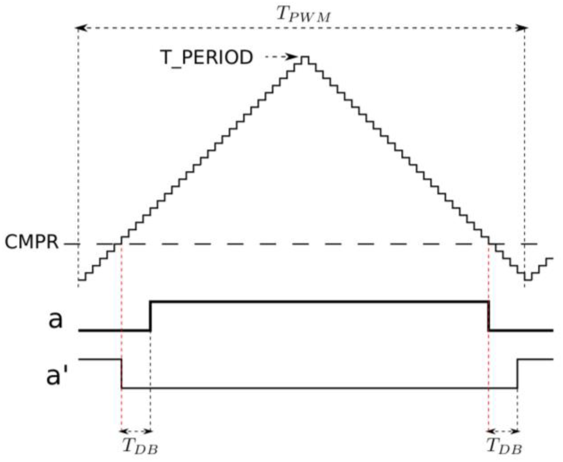
A typical PWM generation process for one branch of the inverter is shown in Figure 17. Where CMPR is the value compared with the content of the timer, T_PERIOD is the value to which the timer counts.

The timer counts clock pulses of period $T_{CLK}=1/f_{CLK}$ in a discrete mode, i.e., using unsigned int numbers. This leads to further errors. The value T_PERIOD to which the timer counts is determined identically for all processors (symmetrical PWM):

$$\mathrm{T}\_\mathrm{PERIOD}=\frac{T_{PWM}}{2·T_{CLK}}=\frac{f_{CLK}}{2·f_{PWM}}$$

(27)

The TMS320F243 processor used in the experiment has $f_{CLK}$= 20 MHz, so it is easy to calculate with what accuracy the timer measures time. For example, if $f_{PWM}$= 2 kHz, then T_PERIOD = 5000, so 5000 is the number of discrete states when measuring time. Thus, the measurement accuracy for the PWM period is 1/5000 (LSB), which is a little more than 12 bits. For such a low frequency, this value is not high.

The maximum value of T_PERIOD, to which the timer counts, changes according to the hyperbolic function when $f_{PWM}$ changes according to formula (27). the function that describes the change in T_PERIOD ($f_{PWM}$) and takes into account the processor clock $f_{CLK}$ is, therefore, extremely simple and requires no approximation:

$$\mathrm{T}\_\mathrm{PERIOD}\left(f_{PWM}\right)=\frac{f_{CLK}/2000}{f_{PWM}}$$

(28)

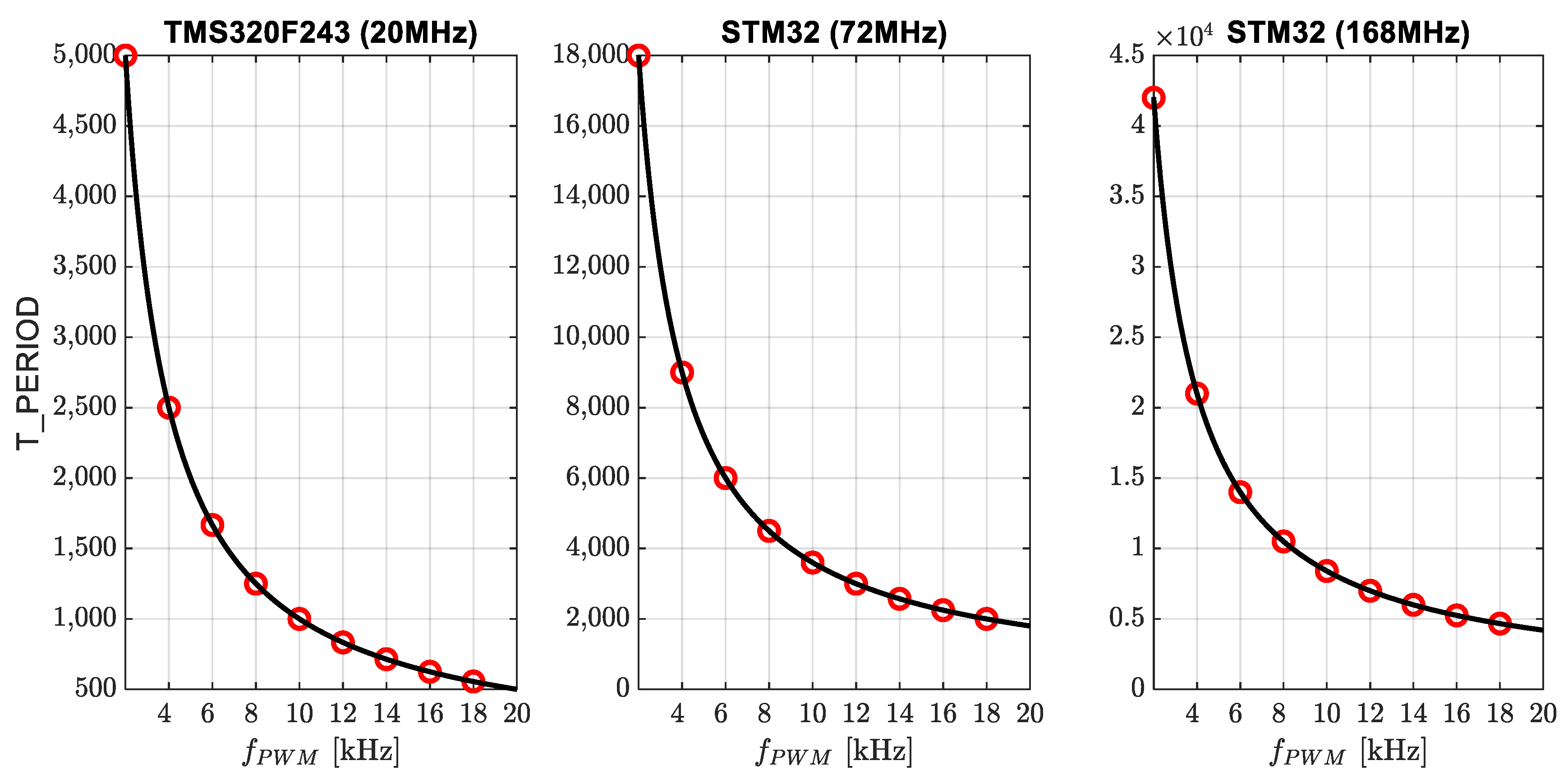
Figure 18 shows a comparison of T_PERIOD values as a function of processor clock frequency. The currently popular processors (STM32) with frequencies higher than 20 MHz are included.

Figure 18 shows the importance of the clock frequency. A comparison for the frequency $f_{PWM}$= 10 kHz reveals (after converting to resolution in bits) that for $f_{CLK}$= 20 MHz, the resolution is about 10 bits; for 72 MHz, it is already less than 12 bits; and for 168 MHz, it is more than 13 bits. These calculations indicate that the clock frequency significantly affects the accuracy of timing and, therefore, the accuracy of PWM generation.

6.5. Comments

The presented results and analysis of the hardware implementation show that the accuracy of voltage generation in VSI is affected by many factors. We have shown, however, that the simulation results represent the first estimate of THD, which is an ideal result to which additional errors, related to the practical implementation of SVPWM control, should be added. Moreover, the results in Figure 9 and Figure 16 are close to each other, which, of course, is due to the accurate implementation of power electronic circuit models in Matlab-Simulink.

7. Conclusions

This article focuses on the induction motor stator current (THD) waveforms, not the RL circuit, as in most publications, which affect the torque ripple.

This paper uses least-squares approximation to determine the THD characteristics of the current and torque ripple $\Delta M_e$ as a function of the $f_{PWM}$ switching frequency of the transistors for VSI. This is a new approach to determining these characteristics that averages out measurement errors. Several VSI approximating functions were proposed, and those with the smallest error were selected.

Dead time $T_{DB}$ in transistor switching was included in the study. Two transistor switching strategies (Pattern #1, Pattern #2) were analyzed, for which the above-mentioned characteristics were determined. Based on simulation results, it can be concluded that the Pattern #1 method gives better results for lower PWM frequencies (up to 10 kHz), while Pattern #2 should be used above 10 kHz.

Experimental tests showed higher-than-expected current THD values, so the analysis of the implementation of SVPWM control based on processors (TMS320 and STM32) was carried out. This analysis shows that the accuracy of the realization (resolution) of the PWM signal depends on the clock frequency that the counter counts. The analysis showed that not at all the highest frequency $f_{PWM}s$ guarantee the lowest THD of current and torque ripple.

Finally, switching losses in the VSI, which are discussed in detail in [6], must also be considered. Our results show that Pattern #2 realizes 33% less switching than Pattern #1, leading to a 50% reduction in VSI losses. Hence, drive systems should be optimized so that THD of current and losses in VSI are as low as possible. Can any general rule of thumb be given? Based on the research, THD of current can be considered satisfactory from 8 kHz onward, and this frequency can be acknowledged optic for drives operating up to 50 Hz.

On the other hand, the results obtained show it can be determined that $f_{PWM }$= 6 kHz is the lowest switching frequency of transistors for which the stator current “resembles “ a sinusoid.

In conclusion, the article presents the following:

• Approximation of THD($f_{PWM}$) and $\Delta M_e\left(f_{PWM}\right)$ characteristics, which, taking into account dead time, present THD changes;
• Two SVPWM modulation methods (Pattern #1, Pattern #2) are compared;
• Experimental results are presented;
• Analysis of PWM hardware implementation.

The obtained results determine that the best THD of the current is in the 8–12 kHz range, which also affects the torque ripple.

The advantage of the proposed method, i.e., using approximation to determine the steady-state characteristics of THD current and torque ripple, is the small number of measurements. Here, there were only nine of them, and the result was the characteristics of the changes in the above parameters, where the argument was the PWM frequency and dead time.

The disadvantage of the results presented here is that eddy currents and steel saturations were not taken into account, as well as losses on associated voltage source inverter operation. These issues are additional topics that can be developed in future publications. In terms of numerical mathematics, non-standard least-squares methods can be used; for example, the Simplex optimization method [43,44] can be used to approximate the presented characteristics.

In addition, the effect of $f_{PWM}$ and $T_{DB}$ on obtaining steady-state operation of electric machine (start-up, loading) dynamics is an interesting topic for future work.

Unfortunately, all these issues could not be presented in this article, but the above proposals provide a place for future research and analysis.

Future work should include issues of the effect of PWM switching frequency on total losses in the drive, i.e., motor eddy currents and losses in the VSI. The research will be able to be extended to analyze the operation of other AC motors.