Optimization of Energy Consumption of Industrial Robots Using Classical PID and MPC Controllers

Abstract

Industrial robots have a key role in the concept of Industry 4.0. On the one hand, these systems improve quality and productivity, but on the other hand, they require a huge amount of energy. Energy saving solutions have to be developed and applied to provide sustainable production. The purpose of this research is to develop the optimal control strategy for industrial robots in order to minimize energy consumption. Therefore, a case study was conducted for the development of two control strategies to be applied to the RV-2AJ Mitsubishi robot arm with 5 DOF, where the system is a nonlinear one. The first examined controller is the classical linear proportional integral derivative (PID) controller, while the second one is the linear model predictive control (MPC) controller. In our study, the performances of both the classical PID model and the linear MPC controller were compared. As a result, it was found that the MPC controller in the execution of the three defined reference trajectories [(1) curve motion, (2) N-shaped motion, and (3) circle motion] was always faster and required less energy consumption, whereas in terms of precision the PID succeeded in executing the trajectory more precisely than the MPC but with higher energy consumption. The main contribution of the research is that the performances of the two control strategies with regard to a complex dynamic system were compared in the case of the execution of three different trajectories. The evaluations show that the MPC controller is, on the one hand, more energy efficient; on the other hand, it provides a shorter cycle time compared to the PID controller.

1. Introduction

Industry 4.0 has caused a paradigm change in production: manufacturing has changed from semi-autonomous to fully autonomous. The industrial sector requires highly adaptive and smart solutions to increase productivity and the quality of the final products. Due to the automation and robotization, human labor can be replaced by machines and industrial robots. On the one hand, these technologies improve quality and productivity, but on the other hand, they consume a huge amount of energy. The current industrial practices are not sustainable with regard to the utilization of resources; therefore, in order to provide sustainable production, energy saving solutions have to be developed and applied [1].

Industrial robot arms are a commonly used system in the automotive industry. Due to the industrial environment scale, these are big systems, with heavy and large mechanical bodies. Consequently, a huge amount of electricity has to be applied to the required torque to move a specific joint. The movement of the joint is executed based on different rules. The first rule is related to the desired trajectory plan of a robot arm in a given workspace, taking into consideration the existing obstacles in this area and the limitations related to the robot arm body arriving at a position [2,3]. The second rule is related to the way in which the actions needed for this mechanical body to follow the desired trajectory with high precision are maintained and processed [3,4]. Recently, scientists have not only focused on the development of trajectory planning and the control field, but also on the optimization of the energy consumption of these robotic systems [5,6].

A study conducted in the United States estimated the increase in the used electrical energy load by 49 million industrial robots to be 22,822 GWh by 2025. This is equivalent to the electricity of all the refrigerators in the northeastern United States in 2009 [7,8]. This increase presents a challenge to scientists who need to research this field and to develop solutions to decrease the electrical energy consumption of the industrial robots and simultaneously provide the high productivity and required precision.

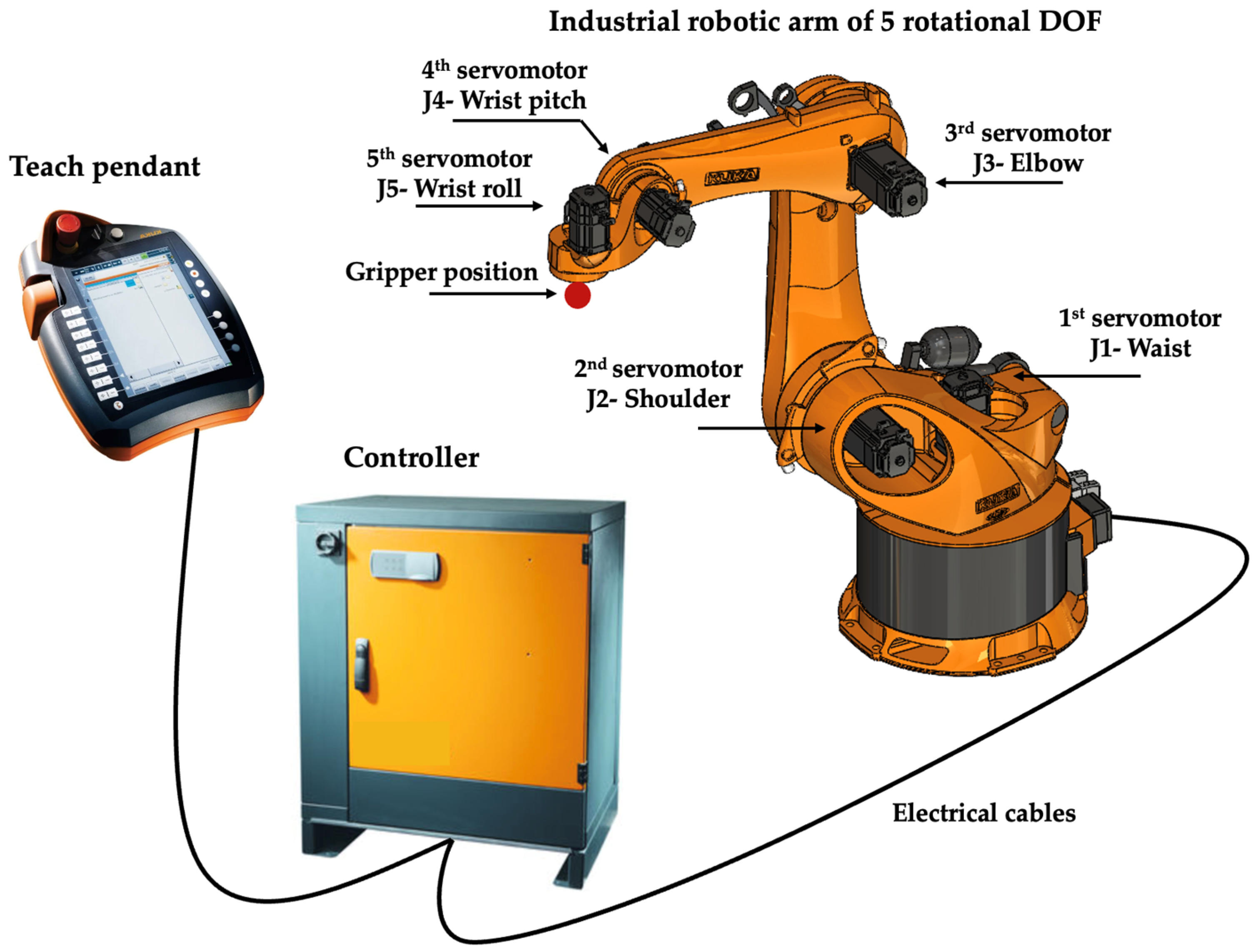
The industrial robot arm—used in the manufacturing processes of the automotive industry—consists of the following components, as presented in Figure 1: mechanical body; robot controller; teach pendant; connecting cables; and software. The process to control the robot arm is based on the received and sent signals from the controller. A desired trajectory or a defined position can be sent to the controller using the teach pendant (manual mode) or by using the software through a script (automatic mode). The controller sends back the commands to the manipulator through electrical cables, where the command signal presents a voltage value that turns on the motors in order to execute the applied torque. A gear box transmission system is connected to the output of the motor in order to increase and double the torque applied on the arm to rotate it. As shown in Figure 1, the most commonly used industrial robot arms have 5 DOF (degrees of freedom) with rotational joints. Due to the high flexibility of such a structure, it can provide a large and complex workspace compared to other constructions. The industrial robot arm’s engine is a servomotor that executes high torque values. The servomotor is an actuator that allows for the precise control of rotational or linear movement, velocity, and acceleration. The application of this type of actuator is highly recommended to maintain the heavy mechanical structure of the robot arm with regard to the gravity effect. A 5 DOF industrial robot arm is depicted in Figure 1, where the number 5 refers to the 5 rotational joints linked between the different bodies. The last joint allows the plugging in of the end effector, which can be of different types for different tasks, i.e., painting, welding, assembling, etc.

The purpose of the detailed explanation above was to highlight the importance of the energy consumption optimization; furthermore, it focused on the question of what might be the effective solution and the main parameters that could have an impact on optimizing the industrial robot arm’s energy consumption.

The aim of our research is to develop the optimal control strategy for industrial robots to minimize the energy consumption. Therefore, a case study was conducted for the development of two controllers to be applied to an RV-2AJ Mitsubishi robot arm with 5 DOF, where the system is a nonlinear one. The first examined controller is the classical linear PID controller, while the second one is the linear MPC controller.

In our study, the performances of both the classical PID model and the linear MPC controller are compared. Compared to previous works [9,10,11], our article also provides a methodology for the MPC controller design, considering the real parameters of the investigated robot arm, the limitations of the linear PID and MPC controllers, and the solutions by which to improve the energy consumption of the robot arm.

As our case study is related to a robot arm with 5 DOF, the system is highly nonlinear. This can be a difficulty and a challenge for the linear MPC controller when predicting the command signal for the five joints simultaneously. Therefore, it is necessary to set a long prediction horizon time in the internal MPC to achieve significant results. The increasing of the prediction horizon time for the MPC controller of the robot arm definitely requires high computational time. There are several approaches in the literature which discuss the improvement possibility for the performance of MPCs using short prediction horizon [12,13]; adaptive predictive horizon [14] is also suggested. Other literature has described solutions leading to the reduction in complexity of the linear MPC [15]. From our perspective, we believe that using the nonlinear MPC with nonlinear constraints in the case of 5 DOF robot arm can achieve more efficient results than the linear MPC. In the case of the nonlinear MPC, the setting of a prediction horizon can be shorter. This approach is highly recommended when the dynamic mathematical model is known [16].

The first part (Section 3.1) of this paper focuses on the detailed methodology relating to the mathematical background of the operation of the RV-2AJ robot arm in order to identify the three mathematical models of the RV-2AJ robot arm: (1) kinematic, (2) Jacobian, and (3) dynamic. We focused on the kinematic model, which is needed to control the desired reference trajectory, where the third model, the “dynamic model”, is needed to simulate the robot arm’s behavior and to build the controllers. The second part (Section 3.2) explains the theoretical backgrounds of both the PID and the linear MPC controllers.

A newly elaborated case study is shown in Section 4 for the design of both the PID and the linear MPC controllers. This part shows the reader how to build the PID and linear MPC controllers and the control loop for the RV-2AJ robot arm in MATLAB Simulink. Suggestions and recommendations are made for tuning the correct controller parameters in the MATLAB Simulink environment.

In Section 5, a detailed comparison is achieved relating to the behavior of both controllers in order to track the motion, minimize the energy consumption, and maintain the stability. The results show the higher energy efficiency of the MPC controller; furthermore, in the case of the application of the PID controller, lower energy consumption can be realized with higher precision.

The main contribution of the research is that the performances of the two control strategies with regard to a complex dynamic system were compared; furthermore, the optimal control strategy was defined in the case of an elaborated case study. It can be concluded that the MPC controller is more flexible in processing the inputs of the desired trajectory and the measured one when executing the command signals. The command signal is presented as a voltage value for the servomotor to execute the right torque for the different joints. By optimizing the command signals, the voltage can be minimized, which results in the minimizing of the torque; therefore, a significant energy saving can be realized.

2. Literature Review—Different Approaches Relating to Energy Saving Operation of Dynamic Systems

According to the literature review, it can be stated that different approaches are available for the energy saving possibilities. It is a fact that if the target is to reduce the electrical energy consumption, the focus has to be on decreasing the acceleration, the jerk, or the torque. Therefore, many scientists focus on studying the trajectory planning of the robot arm, dealing with path optimization to minimize the execution time and the energy consumptions [17,18]. The studies are based on computing the optimal trajectory and finding the best shortcut, while taking into consideration obstacle avoidance in the limited workspace. The solutions are mainly based on developing mathematical optimization and the application of artificial intelligence algorithms, where the trajectory planning problem is always described as a sequential quadratic programming function [19,20]. In references [21,22], the authors presented a new trajectory planning method. This method used particle swarm optimization (PSO) and a Bezier curve interpolation, with which they achieved an energy saving of up to 40%. Števo et al. [23] used a genetic algorithm (GA) for the optimization of a manipulator, where the trajectory was defined as chromosomes composed of a set of points in the robot arm workspace. Wei et al. [24] succeeded in optimizing the desired trajectory and the energy consumption using an artificial neural network (ANN). In the study [25], a hybrid method based on the tabu search algorithm was used to create the optimal path based on the minimum torque applied. Another methodology was used in this context to define the inverse approach based on the prediction of power consumption during the trajectory execution [26,27].

Other studies [28,29] deal with the problem of the energy consumption resulting from the mechanical structure of the robotic arm; therefore, they optimize the shape of the arms to design a lightweight structure that can execute complex tasks. Some authors [30] have focused on the improvement of the electrical part of the robot by dealing with the servo-drivers and merging field-programmable gate array (FPGA) technology in the controller part.

Besides trajectory planification and the body’s structural design, another focus has been raised concerning the control law, as described earlier. The controller loop of the robot arm presents a potential element for the processing of the right commands according to the received inputs. An adequate control strategy can result in time reduction and, at the same time, can decrease the energy consumption [31,32]. The industrial robot arm is a nonlinear dynamic system that requires limited control strategies.

The control approaches of robot arms can be divided into two groups:

• Linear control techniques were initially used in the case of industrial robot arms. These techniques involve applying linear controllers to a linearized model of the system, which is typically derived via a Taylor series expansion and the Jacobian method around an equilibrium point [33].
  In the case study of our paper, the system being considered is a robotic arm executing tasks at low speed. As such a system can be approximated as linear, linear control laws can be applied to it.
• Nonlinear controllers are known as efficient strategies and are applied to an accurate model of the robot arms that considers all the critical nonlinearities of the dynamics. The most commonly used method for controlling industrial robot arms involves the use of nonlinear controllers [34]. Although such controllers can achieve a higher performance with regard to a nonlinear dynamic model of the robotic arm, they require more computational power, which is their main disadvantage. To design a nonlinear control strategy, the dynamic model of the system has to be identified, and in the case of a robot arm with 5 DOF, the model is very complex to calculate [35].

Based on the literature review,

Table 1. Most commonly used control approaches used for industrial robot arms.

Controller Type	Workspace	Linearity Type	Stability and Time Response	Computation Time
PID controller [33,36]	Joint space	Linear	Good stability in low-speed joints, good response time	Medium
Jacobian control “Resolved Motion Control RMC” [37]	Joint space	Nonlinear	Medium stability, slow response time	High
Nonlinear decoupling control [38]	Joint space	Nonlinear	High stability, slow response time	High
Control Lyapunov function [39]	Joint space	Linear or nonlinear	High stability, good response time	High
Passive control [40]	Joint space	Linear or nonlinear	According to the design of the specific system, it can provide high stability, low response time	Very low
Adaptive control [41]	Joint space	Nonlinear	Medium stability within the uncertainties	Can be optimized
Model predictive control (MPC) [42,43]	Joint space	Linear or nonlinear	High stability when the controller is nonlinear, good optimization for different constraints	High but can be optimized
Sliding mode control [44]	Joint space	Nonlinear	High robustness, fast time response	Very high
H-infinity control [45]	Joint space	Linear	High stability and robustness, fast time response	High, depending on the model complexity
Impedance control [46]	Task space	Nonlinear	Good stability when properly tuned, with very fast time response	Very high
Hybrid position force control [47]	Task space	Nonlinear	Good stability when properly tuned, high precision, with very fast time response	Very high

summarizes the most typical linear and nonlinear control strategies used in the control of industrial robot arms [36,37,38,39,40,41,42,43,44,45]. In this research work, the classical PID and the linear MPC approaches are considered in detail to show the main differences and the results obtained from the simulation, especially at the energy consumption level.

The proportional integral derivative (PID) controller [36] is the most commonly applied controller, where the approach is linear; therefore, the right assumption for this control is that the dynamic system should be linear in the case of the robot arm. The dynamic is considered linear while the robot executes the movement in low velocity. Further strategies have been introduced and discussed in the literature: the backstepping control [48], the linear and nonlinear model predictive control (MPC) [49,50,51], the adaptive control [41], and the slide mode control. In addition to the precise and smooth execution of the desired trajectory, minimizing the energy consumption can also be realized by the right control strategy, where a cost function of the energy usage is added to the controller. Therefore, the criteria focus not only on computing the error between the desired position and the obtained one, but also on minimizing the cost function with regard to the energy, which is presented as the applied torque on the joints. Nonoyama et al. [52] provided a solution to reduce the energy consumption of a dual robot arm. Their suggested approach is based on tuning the gains of the PID controller using metaheuristic approaches, i.e., GA and PSO.

Our paper focuses on the application of the classical PID and MPC strategies. A lot of research related to the energy saving of different complex systems has shown that the MPC controller was always able to maintain the variation of the command signal in order to precisely track the target with minimal energy consumption [53,54,55]. In [54], the authors applied the MPC to control a radiant floor heating system. The study resulted in the MPC demonstrating the ability to save time and energy consumption. In terms of time saving, the MPC reduces the response time by about 56% compared to that of the PID controller, whereas in terms of energy consumption, the MPC controller can effectively reduce the energy consumption by 14.9% when maintaining the air-source pump compared to that of the application of the PID controller.

The MPC uses a predictive model of the dynamic system to determine the optimal control output over a finite time horizon. Future changes in the controlling of a dynamic system have an effect on the optimization of the control input over time, leading to potentially greater energy savings. However, MPC controllers are more complex and computationally intensive than PID controllers, and they require accurate models of the dynamic systems to work effectively [56]. One limitation of the MPC is related to the prediction horizon. If this parameter is too small, it will result in myopic decisions, and if the parameter is too big, it will require a higher computational time.

3. Materials and Methods

The main purpose of the study is to compare the performances of two control strategies in the case of an industrial robot arm: the proportional integral derivative (PID) and the model predictive control (MPC). In particular, the study focuses on the Mitsubishi RV-2AJ robotic arm, which has 5 degrees of freedom. As the model of the controller relies on the robot’s mathematical dynamic model and its essential variables, the article provides a newly developed procedure for improving an appropriate control approach and takes the following steps into consideration:

• Identification of the dynamic mathematical model using the real parameters of an RV-2AJ robot arm;
• Application of both the PID and the linear model predictive control techniques;
• A detailed comparison of both controller strategies to demonstrate the efficiency of the MPC and the classical PID controller in optimizing energy consumption.

The simulation of the investigated control models was carried out using MATLAB Simulink software, which provides various tools to achieve the research objective effectively. Using Simulink is particularly advantageous because setting the parameters and analyzing the results is easier compared to the application of MATLAB Script.

This paper outlines the methods used to build both models. First, the modeling of the dynamics of the RV-2AJ robot arm is highlighted; then, the control strategy is developed. The paper demonstrates the use of the PID and model predictive controllers in general and demonstrates how both controllers can be successfully tuned.

3.1. Mathematical Modeling of RV-2AJ Robot Arm

To control the movement of RV-2AJ robot arms effectively in an industrial environment, it is necessary to conduct a dynamic analysis of the specific robot arm to create accurate mathematical models. The analysis involves several mathematical representations, which include the following:

• The homogeneous transformation matrices through the task space and the joint space;
• The forward and inverse kinematic models that describe the position and the angles, respectively;
• The Jacobian matrices that describe the velocity of the end effector of the robot arm gripper in relation to the joint velocities;
• The dynamic models that define the equations related to the movement of the robot arm. These models demonstrate the relationships between the torques applied by the motors and the accelerations, velocities, and positions of the joints [36,57].

Figure 2 presents the mechanical body of the RV-2AJ robot arm, including the 5 rotational joints.

3.1.1. Forward and Inverse Kinematic Models of RV-2AJ Robot Arm

To describe the physical characteristics of robots in a systematic manner, various approaches have been developed. Among these, the widely used method is the one formulated by Denavit–Hartenberg [36], which is suitable only for industrial robot arms with an open-chain serial structure. The robot arm RV-2AJ is a serial type which has an open-chain configuration, comprising 6 links and 5 rotational joints. The Denavit–Hartenberg approach is based on calculating the homogeneous transformation matrix (H) that defines the frame Rj relative to another frame R_j−1, as described below, where j stands for the number of joints:

$${\mathbf{H}}_j^{j-1}=\mathrm{R}\mathrm{o}\mathrm{t}(\mathbf{x},{\alpha }_j)\mathrm{T}\mathrm{r}\mathrm{a}\mathrm{n}\mathrm{s}(\mathbf{x},d_j)\mathrm{R}\mathrm{o}\mathrm{t}(\mathbf{z},{\theta }_j)\mathrm{T}\mathrm{r}\mathrm{a}\mathrm{n}\mathrm{s}(\mathbf{z},r_j)$$

(1)

$${\mathbf{H}}_j^{j-1}=\left(\begin{array}{cc}\begin{array}{cc}Cos{\theta }_j& -Sin{\theta }_j\\ Cos{\alpha }_{j}Sin{\theta }_j& Cos{\alpha }_{j}Cos{\theta }_j\end{array}& \begin{array}{cc}0& d_j\\ -Sin{\alpha }_j& -r_{j}Sin{\alpha }_j\end{array}\\ \begin{array}{cc}Sin{\alpha }_{j}Cos{\theta }_j& Sin{\alpha }_{j}Cos{\theta }_j\\ 0& 0\end{array}& \begin{array}{cc}Cos{\alpha }_j& r_{j}Cos{\alpha }_j\\ 0& 1\end{array}\end{array}\right)$$

(2)

where

-

${\alpha }_j$: the angle between ${\mathbf{z}}_{j-1}$ and ${\mathbf{z}}_j$ about ${\mathbf{x}}_{j-1}$;

-

$d_j$: the distance between ${\mathbf{z}}_{j-1}$ and ${\mathbf{z}}_j$ along ${\mathbf{x}}_{j-1}$;

-

${\theta }_j$: the angle between ${\mathbf{x}}_{j-1}$ and ${\mathbf{x}}_j$ about ${\mathbf{z}}_j$;

-

$r_j$: the distance between ${\mathbf{x}}_{j-1}$ and ${\mathbf{x}}_j$ along ${\mathbf{z}}_j$.

Furthermore, the rotation matrix ${\mathbf{A}}_j^{j-1}$(3 × 3) can be obtained as:

$${\mathbf{A}}_j^{j-1}=Rot(\mathbf{x},{\alpha }_j)Rot(\mathbf{z},{\theta }_j)$$

(3)

Forward Kinematics of RV-2AJ Robot Arm

To ensure convenient computation during the forward and inverse kinematics processes, it is recommended to align the three axes (R₀, R₁, R₂) and the two axes (R₄, R₅); this is illustrated in Figure 3.

Figure 3 shows the frame assignments of the rotational joints of the RV-2AJ robot arm.

Table 2. Parameters of Denavit–Hartenberg with regard to the RV-2AJ robot arm.

jth Joints	Axes	θj	dj	αj	rj
1	R0−R1	θ1	0	0	r01
2	R1–R2	θ2	0	π/2	0
3	R2–R3	θ3	d23	0	0
4	R3–R4	θ4	d34	0	0
5	R4–R5	θ4	0	π/2	r45

was created based on this morphological description, which describes the Denavit–Hartenberg parameters for the RV-2AJ robot arm.

The homogeneous transformation matrix from the first link to the last link, which is the end effector, is written as follows:

$${\mathbf{H}}_5^0={\mathbf{H}}_1^0·{\mathbf{H}}_2^1·{\mathbf{H}}_3^2·{\mathbf{H}}_4^3·{\mathbf{H}}_5^4$$

(4)

As a result, a matrix of (4 × 4) is obtained, the fourth column describes the position vector that locates the end effector:

$${\mathbf{H}}_5^0=\left(\begin{array}{cc}\begin{array}{cc}{s}_x& n_x\\ s_y& n_y\end{array}& \begin{array}{cc}{a}_x& P_x\\ a_y& P_y\end{array}\\ \begin{array}{cc}{s}_z& n_z\\ 0& 0\end{array}& \begin{array}{cc}{a}_z& P_z\\ 0& 1\end{array}\end{array}\right)$$

(5)

where s_x, s_y, n_x, n_y, n_z, a_x, a_y, and a_z are the elements of the rotational matrix ${\mathbf{A}}_j^{j-1}$ that describe the orientation according to the x, y, and z axes; P_x, P_y, and P_z are the position vectors.

Inverse Kinematics of RV-2AJ Robot Arm

The inverse problem involves the determination of the coordinated joints that correspond to the end effector’s position data. If available, the inverse geometry model provides an explicit form that offers all feasible solutions. In order to create the inverse geometry model for the RV-2AJ robot arm, Paul’s method [36] is applied in the research. This method is advantageous because it enables us to handle each unique scenario individually and is well suited to most industrial robots.

The homogeneous transformation matrix is the following:

$${\mathbf{H}}_5^0={\mathbf{H}}_1^0\left({\theta }_1\right)·{\mathbf{H}}_2^1\left({\theta }_2\right)·{\mathbf{H}}_3^2\left({\theta }_3\right)·{\mathbf{H}}_4^3\left({\theta }_4\right)·{\mathbf{H}}_5^4\left({\theta }_5\right)$$

(6)

We assume that the desired position (U₀) (is known, with a known orientation matrix and position vector where:

$${\mathbf{H}}_5^0=\left(\begin{array}{cc}\begin{array}{cc}{s}_x& n_x\\ s_y& n_y\end{array}& \begin{array}{cc}{a}_x& P_x\\ a_y& P_y\end{array}\\ \begin{array}{cc}{s}_z& n_z\\ 0& 0\end{array}& \begin{array}{cc}{a}_z& P_z\\ 0& 1\end{array}\end{array}\right)={\mathbf{U}}_0$$

(7)

We try to solve the following system of equations:

$${\mathbf{U}}_0={\mathbf{H}}_1^0\left({\theta }_1\right)·{\mathbf{H}}_2^1\left({\theta }_2\right)·{\mathbf{H}}_3^2\left({\theta }_3\right)·{\mathbf{H}}_4^3\left({\theta }_4\right)·{\mathbf{H}}_5^4\left({\theta }_5\right)$$

(8)

Paul [33] proposed a method to calculate ${\theta }_1,{\theta }_2,{\theta }_3$, that is based on pre-multiplying successively the two elements of Equation (6) by the matrices ${\mathbf{H}}_{j-1}^j$ for j changing from 1 to 4. These multiplications help to identify, one by one, the joint variables that we are searching for.

To calculate ${\theta }_4 \mathrm{a}\mathrm{n}\mathrm{d} {\theta }_5,$ the desired orientation matrix ${\mathbf{A}}_{j-1}^j$ is used because the two angles ${\theta }_4 \mathrm{a}\mathrm{n}\mathrm{d} {\theta }_5$ refer to the orientation of the end effector of the robot arm.

The successive pre-multiplication identifies a system of equations in a function of the desired elements of the position vector $P_x$, $P_y,$ and $P_z$ and the desired elements of the desired orientation matrix $s_x$, $s_y$, $s_z$, $n_x$, $n_y$, $n_z$, $a_x$, $a_y,a_z$.

3.1.2. Jacobian and Dynamic Models of the RV-2AJ Robot Arm

The Jacobian matrix presents a key function—beside the dynamic model—in order to have a faster simulation. This matrix helps the software to calculate the singularities of the provided trajectory or to converge to the solution of the dynamic equation that calculates the torque applied on every joint.

The simplest Jacobian matrix of the RV-2AJ robot arm, using the Renaud method [36], is as follows, where it describes the differential displacement of the position of the end effector X in terms of the differential variation of the joint variables q:

$$\mathbf{J}=\frac{\partial X}{\partial q}$$

(9)

In this paper, the kinematic singularity problems are not addressed because we are not looking for generated random trajectories, where generally the singularity problems should be addressed. The main goal of our research is to find the optimal control strategy for the robot arm to execute a well-defined motion while minimizing the energy consumption. In Section 5, three different motions [(1) a semi-curve motion, (2) an N-shaped motion, and (3) a circle motion] are generated to construct the path in the limited workspace of the RV-2AJ robot arm.

The design, operation, and simulation of the robot arms are based on their dynamic models, which can be classified into two types [57,58]:

• The inverse dynamic model describes the joint torques and forces in the function of the joint positions, velocities, and accelerations;
• The direct dynamic model describes the joint accelerations in the function of the joint positions, velocities, and torques.

In the case of the robot arm’s control simulation and operation, the inverse dynamic model is required for the calculation of the torque actuator for every joint. The computation of the inverse dynamic model is based on a dedicated computational algorithm.

Several dedicated computational algorithms are available in the literature. In the case of our type of investigated RV-2AJ robot arm, the most often used algorithms are:

• Lagrange formalism;
• Newton–Euler formalism.

Lagrange formalism is required to calculate the inertia matrices, Coriolis vector, and gravity vector, while Newton–Euler formalism is used to calculate the torque joints; the Lagrange method cannot provide the best performing model in terms of the number of transactions during the torque calculation.

In order to simulate and control the motion of the RV-2AJ robot arm in the case of the application of both the PID and the MPC controllers in MATLAB 2022 software, both of the previously dedicated computations should be performed. In our research, the focus is mainly on calculating the forward and inverse kinematics beside the Jacobian matrix. The dynamic model used for the RV-2AJ robot arm is presented as a CAD model created by SolidWorks software. SolidWorks can provide us with the ability to generate the inertia matrix automatically for various mechanical body structures, e.g., for the RV-2AJ robot arm. Additionally, the software enables us to import the entire mechanical body structure into the Simscape body toolbox of MATLAB software, which is a powerful tool that allows us to calculate the torques of the joints.

Using MATLAB Simulink, the block function that contains the dynamic model can test the robot’s movements and behaviors in a virtual environment before deploying it in the real world. This can help to identify any potential problems or limitations before they arise. From this model, the torques and accelerations can be calculated by direct and inverse dynamic equations.

3.2. Control Strategies for RV-2AJ Robot Arm

The mathematical algorithm known as the controller system is responsible for determining how the robot arm should move in order to follow a particular trajectory based on a set point. While the principle behind this system is relatively straightforward, designing it requires special attention due to the complex dynamics of the system. There is a lot of literature in this field that can provide insights into the effectiveness of the suggested controllers. The next part focuses on a detailed description of the application of the classical PID and the linear MPC in the case of industrial robot arms.

3.2.1. The Classical PID for RV-2AJ Robot Arm

A proportional integral derivative (PID) controller is a closed control loop with a feedback signal to regulate a process by continuously measuring an error signal and adjusting the control signal to minimize the error. The controller consists of three terms [33]:

• The proportional term (P): The proportional term executes an output that is proportional to the error signal. The larger the error, the larger the output. The proportional term alone can produce a stable system, but it may not eliminate the steady-state error.
• The integral term (I): The integral part is responsible for the sum of the instantaneous error with regard to time. The integral term is used to eliminate the steady-state error in the system response; moreover, it stabilizes the dynamic system.
• The derivative term (D): The derivative part is responsible for executing the rate of change of the error signal. This term is used to achieve a fast response in the dynamic system, reducing overshoot and settling time.

As shown in Equation (10), the obtained signal u(t) in the PID controller is the sum of the three terms: the proportional K_p, the integral K_I, and the derivative K_d. These constant gains are adjusted to obtain the desired system response, where e is the error between the desired and the measured signals [36].

$$u\left(t\right)=K_{P}e\left(t\right)+K_I{\int }_{t0}^{t}e\left(t\right)dt+K_d\frac{de\left(t\right)}{dt}$$

(10)

This method is utilized for a robot arm equipped with powerful reduction ratio servomotors. If the system exhibits linear behavior, traditional control techniques can be utilized to achieve movement control.

The robot arm’s dynamic model consists of n second-order nonlinear and coupled differential equations, where n represents the number of joints. In the traditional control theory, the robot dynamic was assumed to be a linear model, where every joint was controlled by a decentralized PID controller. The advantages of this approach are the low computational time and the ease of applicability. At the same time, it can result in poor tracking accuracy and setpoint overruns during rapid movements, as well as temporal response variations depending on the robot’s configuration. Nonetheless, in many practical applications, these limitations are not significant issues. Figure 4 depicts the command scheme for this approach.

For the RV-2AJ robot arm, the control equation is given as follows:

$${\tau }_j={\mathbf{K}}_{\mathit{p}}\left(q_d-q\right)+{\mathbf{K}}_{\mathit{d}}\left({\dot{q}}_d-\dot{q}\right)+{\mathbf{K}}_{\mathit{I}}{\int }_{t_0}^t\left(q_d-q\right)dt$$

(11)

where

-

$q_d$ and ${\dot{q}}_d$ are the desired position and velocity vectors in the joint space;

-

${\mathbf{K}}_{\mathit{p}}$, ${\mathbf{K}}_{\mathit{d}}$, and ${\mathbf{K}}_{\mathit{I}}$ form the positive diagonal matrices of the (5 × 5) dimension.

The PID controller gains $K_{pj}$, $K_{dj}$, and $K_{Ij}$ for every joint j are calculated using the following formula in Equation (12):

$$\begin{array}{c}{K}_{pj}=3a_j{{\omega }_j}^2\\ K_{dj}+F_{dj}=3a_j{\omega }_j\\ K_{Ij}=a_j{{\omega }_j}^3\end{array}$$

(12)

where

-

$a_j$ = max ($A_{jj})$ is the maximum of the inertia matrix element $A_{jj}$ of the RV-2AJ robot;

-

${\omega }_j$ is the pulsation of the robotic system, and we assume that ${\omega }_j=1.25$ rad/s;

-

$F_{vj}$ is the viscous friction, and in our case, this parameter is neglected.

The elements of the inertia matrix $\mathbf{A}$ in the case of this paper are ($A_{11}$, $A_{22}$, $A_{33}$, $A_{44}$, $A_{55}$) and are taken from the dynamic model using SolidWorks software.

3.2.2. Linear MPC for RV-2AJ Robot Arm

The linear MPC is an advanced technique used to control automated processes, primarily in an industrial environment. The MPC is designed to use a dynamic model of the system, which can be linear or nonlinear, to predict the system response in the future. The fundamental characteristic of the MPC is the online calculation of the output, which involves optimizing the input/output values through an objective function to forecast future behavior. The MPC controller executes this prediction through an internal model over a finite time window, known as the prediction horizon. The optimization problem’s solution is then presented as a control signal. As the data in the controller are updated, in the next interval the controller can resolve the optimization problem; thus, the MPC is also known as the optimal controller of a moving horizon.

One common approach to the linear MPC is to use a linearized model, which is simpler and faster when executing the necessary command inputs for the robot arm. However, for highly nonlinear systems such as a robot arm, the linearized model may not accurately capture the behavior of the system and may result in suboptimal control performance; therefore, it is recommended that the parameters of this controller should be chosen properly to achieve good results.

The MPC is a method for solving an optimization task, using a “Quadratic Program (QP)” algorithm, which involves three main elements:

-

a dynamic state model;

-

an objective function to be achieved;

-

constraints that set limitations through boundaries for the future response; these constraints are either soft or hard.

The plant model of the MPC is an open loop. Customization of the MPC is based on setting a prediction horizon P and a control horizon N. These two parameters are necessary to minimize the objective function and to compute the set of control inputs u_k, …, u_k+N−1 and the upcoming states x_k+1, …, x_k+N. The objective function is subject to the inputs and the state spaces of the dynamic model. The first element of the set of calculated inputs (u_k) is used as the input to the robot arm, and the sequence of calculations is repeated in the next iterations [59,60,61].

The MPC controller evaluates a number of intervals for future control in order to optimize the actual control inputs. This number is called the prediction horizon P.

N is the number of the steps of the control inputs to be optimized at the control interval k. The control horizon is always in the range of 1 and P.

The effectiveness of the MPC has been demonstrated to be efficient in applications with short sampling periods and has provided good results in terms of speed and accuracy in the field of numerical control [42,43]. On the other hand, the MPC presents a significant drawback with regard to the higher computation time.

Figure 5 presents the closed control loop of the internal scheme of the MPC with regard to the RV-2AJ robot arm, where the reference trajectory signal is ref(t), y₀(t) is the initial state signal, y(t) is the measured signal, c(t) is the command signal, and dist(t) is the disturbance signal, if it exists.

Figure 6 illustrates the concept of the internal actions of the MPC [27].

The cost function $(\Theta$) generally comprises four terms, with each term specifically targeting a different aspect of the controller’s performance. In essence, each term within $\Theta$ describes an objective sub-function:

$$\Theta \left({\mathcal{z}}_k\right)={\Theta }_y\left({\mathcal{z}}_k\right)+{\Theta }_u\left({\mathcal{z}}_k\right)+{\Theta }_{∆u}\left({\mathcal{z}}_k\right)+{\Theta }_{\epsilon }\left({\mathcal{z}}_k\right)$$

(13)

where

-

${\Theta }_y\left({\mathcal{z}}_k\right)$: output reference tracking cost function;

-

${\Theta }_u\left({\mathcal{z}}_k\right)$: manipulated variable tracking cost function;

-

${\Theta }_{∆u}\left({\mathcal{z}}_k\right)$: manipulated variable movement suppression cost function;

-

${\Theta }_{\epsilon }\left({\mathcal{z}}_k\right)$: constraint violation cost function;

-

${\mathcal{z}}_k$: the quadratic function.

The main objective in this case was to reduce the values of ${\Theta }_y\left({\mathcal{z}}_k\right)$ and ${\Theta }_u\left({\mathcal{z}}_k\right)$. To achieve the desired output, it was necessary to minimize the variance between the reference signal r(t) and the output signal y(t). This resulted in the minimization of the second term, which ensures that the controller selects manipulated variables (MVs) that are close to the target values. Typically, the statement of the problem is formulated as:

$$\underset{u_t,....,u_{t+N-1}}{\min }\left\{\sum _{k=0}^{N-1}{‖r\left(t\right)-y_{t+k}‖}^2+\rho {‖u_{t+k}-u_r\left(t\right)‖}^2\right\}$$

(14)

subject to:

-

$x_{t+k+1}=f(x_{t+k},u_{t+k})$, which defines the dynamic of the robot arm;

-

$r\left(t\right)$ defines the reference trajectory signal;

-

$y_{t+k}=g(x_{t+k},u_{t+k})$, which defines the outputs of the robot arm;

-

$u_{min}\le u_{t+k}\le u_{max}$;

-

$y_{min}\le y_{t+k}\le y_{max}$;

-

$x_t=x\left(t\right)$,$k=0,\dots ,N-1$, which defines the state variables.

The next section will show how the linear MPC designs can be created using MATLAB software. The software offers various features for resolving energy modeling issues in research with the use of the Simscape toolbox. The MPC controller in the MATLAB environment enables the selection of appropriate parameters for adjusting the controller based on the robot arm model. Within the available methods, the linear MPC can be differentiated, where a quadratic program is employed to manage the optimization problem at each control interval for the future. The outcome specifies the manipulated variables that have to be applied in the dynamic system of the robot arm until the subsequent sampling period. Regarding the following scenario, the defined objective function in the software is written as:

$$\Theta \left({\mathcal{z}}_k\right)={\Theta }_y\left({\mathcal{z}}_k\right)+{\Theta }_u\left({\mathcal{z}}_k\right)$$

(15)

$$\begin{gathered} \Theta \left({\mathcal{z}}_k\right)=\sum _{j=1}^{n_y}\sum _{i=1}^p\left[{\left\{\frac{w_{i,j}^y}{s_j^y}\left[r_j\left(k+i\left|k\right.\right)-y_j\left(k+i\left|k\right.\right)\right]\right\}}^2 \\ \hspace{1em}\hspace{1em}\hspace{1em}\hspace{1em}\hspace{1em}\hspace{1em}\hspace{1em}\hspace{1em}\hspace{1em}+{\left\{\frac{w_{i,j}^y}{s_j^y}\left[u_j\left(k+i\left|k\right.\right)-u_{j,target}\left(k+i\left|k\right.\right)\right]\right\}}^2\right] \end{gathered}$$

(16)

where $k$ is the actual sampling period; $p$ is the prediction horizon that presents the length of the intervals; and $n_y$ is the number of the output variables of the robot arm. ${\mathcal{z}}_k$ is the quadratic function, in MATLAB ${\epsilon }_k$ is a floating-point relative accuracy, given by:

$${{\mathcal{z}}_k}^T=\left[{u\left(k\left|k\right.\right)}^T{u(k+1\left|k\right.)}^T\dots {u\left(k+p-1\left|k\right.\right)}^T{\epsilon }_k\right]$$

(17)

where at the i-th prediction horizon step:

-

$y_j\left(k+i\left|k\right.\right)$ presents the forecasted value of the j-th robot arm output;

-

$r_j\left(k+i\left|k\right.\right)$ presents the desired value for the j-th robot arm output;

-

$s_j^y$ presents the scale factor for the j-th robot arm output;

-

$w_{i,j}^y$ presents the tuning weight for the j-th robot arm output (dimensionless).

The advantage of the linear MPC is that the controller supports the use of the cost functions that are not specific to a particular application. These functions can be formulated by combining nonlinear or linear functions that operate on the system’s states and inputs. In order to optimize performance, an analytical Jacobian matrix can also be defined for the cost function in order to enhance computational efficiency. By utilizing a cost function, the linear MPC algorithm can achieve the dual goals of maximizing profitability while simultaneously minimizing energy consumption. On the other hand, the MPC provides the choice to set the boundaries for the inputs’ system, which make it advantageous in minimizing the energy consumption.

4. Case Study—Modelling and Simulation of the Investigated RJ-2AJ Robot Arm

In this section, the investigated strategies of the modeling and control parts for the RV-2AJ robot arm are described. In our case study, the distances of the links of the RV-2AJ robot arm are the following: d₂₃ = 250 mm and d₃₄ = 160 mm; r₀₁ and r₄₅ are considered equal to 0.

4.1. Modeling of the Investigated RV-2AJ Robot Arm

4.1.1. Forward Kinematic of RV-2AJ robot arm

The calculated homogeneous transformation matrix between two joints j-1 and j are as follows in our case study:

$$\begin{gathered} {\mathbf{H}}_1^0=\left(\begin{array}{cc}\begin{array}{cc}Cos\left(\theta 1\right)& -Sin\left(\theta 1\right)\\ \begin{array}{c}Sin\left(\theta 1\right)\\ 0\\ 0\end{array}& \begin{array}{c}Cos\left(\theta 1\right)\\ 0\\ 0\end{array}\end{array}& \begin{array}{cc}0& 0\\ \begin{array}{c}0\\ 1\\ 0\end{array}& \begin{array}{c}0\\ r_{01}\\ 1\end{array}\end{array}\end{array}\right)\hspace{1em}\hspace{1em}{\mathbf{H}}_2^1=\left(\begin{array}{cc}\begin{array}{cc}Cos\left(\theta 2\right)& -Sin\left(\theta 2\right)\\ \begin{array}{c}0\\ Sin\left(\theta 2\right)\\ 0\end{array}& \begin{array}{c}0\\ Cos\left(\theta 2\right)\\ 0\end{array}\end{array}& \begin{array}{cc}0& 0\\ \begin{array}{c}-1\\ 1\\ 0\end{array}& \begin{array}{c}0\\ 0\\ 1\end{array}\end{array}\end{array}\right) \\ {\mathbf{H}}_3^2=\left(\begin{array}{cc}\begin{array}{cc}Cos\left(\theta 3\right)& -Sin\left(\theta 3\right)\\ \begin{array}{c}Sin\left(\theta 3\right)\\ 0\\ 0\end{array}& \begin{array}{c}Cos\left(\theta 3\right)\\ 0\\ 0\end{array}\end{array}& \begin{array}{cc}0& d_{23}\\ \begin{array}{c}0\\ 1\\ 0\end{array}& \begin{array}{c}0\\ 0\\ 1\end{array}\end{array}\end{array}\right)\hspace{1em}\hspace{1em}{\mathbf{H}}_4^3=\left(\begin{array}{cc}\begin{array}{cc}Cos\left(\theta 4\right)& -Sin\left(\theta 4\right)\\ \begin{array}{c}Sin\left(\theta 4\right)\\ 0\\ 0\end{array}& \begin{array}{c}Cos\left(\theta 4\right)\\ 0\\ 0\end{array}\end{array}& \begin{array}{cc}0& d_{34}\\ \begin{array}{c}0\\ 1\\ 0\end{array}& \begin{array}{c}0\\ 0\\ 1\end{array}\end{array}\end{array}\right) \\ {\mathbf{H}}_5^4=\left(\begin{array}{cc}\begin{array}{cc}Cos\left(\theta 5\right)& -Sin\left(\theta 5\right)\\ \begin{array}{c}0\\ -Sin\left(\theta 5\right)\\ 0\end{array}& \begin{array}{c}0\\ -Cos\left(\theta 5\right)\\ 0\end{array}\end{array}& \begin{array}{cc}0& 0\\ \begin{array}{c}1\\ 0\\ 0\end{array}& \begin{array}{c}{r}_{45}\\ 0\\ 1\end{array}\end{array}\end{array}\right) \end{gathered}$$

(18)

The position vector for the RV-2AJ robot arm is the following:

$$\begin{array}{c}{P}_{\mathrm{x}}=250Cos\left(\theta 1\right)Cos\left(\theta 2\right)+160Cos\left(\theta 1\right)Cos\left(\theta 2\right)Cos\left(\theta 3\right)-160Cos\left(\theta 1\right)Sin\left(\theta 2\right)Sin\left(\theta 3\right)\\ P_{\mathrm{y}}=250Cos\left(\theta 2\right)Sin\left(\theta 1\right)+160Cos\left(\theta 2\right)Cos\left(\theta 3\right)Sin\left(\theta 1\right)-160Sin\left(\theta 1\right)Sin\left(\theta 2\right)Sin\left(\theta 3\right)\\ P_{\mathrm{z}}=250Sin\left(\theta 2\right)+160Cos\left(\theta 2\right)Sin\left(\theta 3\right)+160Cos\left(\theta 3\right)Sin\left(\theta 2\right)\end{array}$$

(19)

The orientation matrix is the following:

$$\begin{array}{c}{\mathrm{s}}_{\mathrm{x}}=Cos\left(\theta 5\right)(Cos\left(\theta 4\right)\left(Cos\left(\theta 1\right)Cos\left(\theta 2\right)Cos\left(\theta 3\right)-Cos\left(\theta 1\right)Sin\left(\theta 2\right)Sin\left(\theta 3\right)\right)-Sin\left(\theta 4\right)\left(Cos\left(\theta 1\right)Cos\left(\theta 2\right)Sin\left(\theta 3\right)+Cos\left(\theta 1\right)Cos\left(\theta 3\right)Sin\left(\theta 2\right)\right)-Sin(\theta 1)Sin\left(\theta 5\right)\\ {\mathrm{s}}_{\mathrm{y}}=Cos\left(\theta 5\right)(Cos\left(\theta 4\right)\left(Cos\left(\theta 2\right)Cos\left(\theta 3\right)Sin\left(\theta 1\right)-Sin\left(\theta 1\right)Sin\left(\theta 2\right)Sin\left(\theta 3\right)\right)-Sin\left(\theta 4\right)\left(Cos\left(\theta 2\right)Sin\left(\theta 1\right)Sin\left(\theta 3\right)+Cos\left(\theta 3\right)Sin\left(\theta 1\right)Sin\left(\theta 2\right)\right)+Cos(\theta 1)Sin\left(\theta 5\right)\\ \begin{array}{c}{\mathrm{s}}_{\mathrm{z}}=Cos\left(\theta 5\right)(Cos\left(\theta 4\right)\left(Cos\left(\theta 2\right)Sin\left(\theta 3\right)+Cos\left(\theta 3\right)Sin\left(\theta 2\right)\right)-Sin(\theta 4)\left(Sin\left(\theta 2\right)Sin\left(\theta 3\right)-Cos\left(\theta 2\right)Cos\left(\theta 3\right)\right)\\ {\mathrm{n}}_{\mathrm{x}}=-Sin\left(\theta 5\right)(Cos\left(\theta 4\right)\left(Cos\left(\theta 1\right)Cos\left(\theta 2\right)Cos\left(\theta 3\right)-Cos\left(\theta 1\right)Sin\left(\theta 2\right)Sin\left(\theta 3\right)\right)-Sin\left(\theta 4\right)\left(Cos\left(\theta 1\right)Cos\left(\theta 2\right)Sin\left(\theta 3\right)+Cos\left(\theta 1\right)Cos\left(\theta 3\right)Sin\left(\theta 2\right)\right)-Cos(\theta 5\left)Sin\right(\theta 1)\\ \begin{array}{c}{\mathrm{n}}_{\mathrm{y}}=Cos\left(\theta 1\right)Cos\left(\theta 5\right)-Sin\left(\theta 5\right)(Cos\left(\theta 4\right)\left(Cos\left(\theta 2\right)Cos\left(\theta 3\right)Sin\left(\theta 1\right)-Sin\left(\theta 1\right)Sin\left(\theta 2\right)Sin\left(\theta 3\right)\right)-Sin\left(\theta 4\right)\left(Cos\left(\theta 2\right)Sin\left(\theta 1\right)Sin\left(\theta 3\right)+Cos\left(\theta 3\right)Sin\left(\theta 1\right)Sin\left(\theta 2\right)\right)\\ \begin{array}{c}{\mathrm{n}}_{\mathrm{z}}=-Sin\left(\theta 5\right)\left(Cos\left(\theta 4\right)(Cos\left(\theta 2\right)Sin\left(\theta 3\right)+Cos\left(\theta 3\right)Sin\left(\theta 2\right))\right)-Sin\left(\theta 4\right)\left(Sin\left(\theta 2\right)Sin\left(\theta 3\right)-Cos\left(\theta 2\right)Cos\left(\theta 3\right)\right)\\ {\mathrm{a}}_{\mathrm{x}}=-Cos\left(\theta 4\right)\left(Cos\left(\theta 1\right)Cos\left(\theta 2\right)Sin\left(\theta 3\right)+Cos\left(\theta 1\right)Cos\left(\theta 3\right)Sin\left(\theta 2\right)\right)-Sin\left(\theta 4\right)\left(Cos\left(\theta 1\right)Cos\left(\theta 2\right)Cos\left(\theta 3\right)-Cos\left(\theta 1\right)Sin\left(\theta 2\right)Sin\left(\theta 3\right)\right)\\ \begin{array}{c}{\mathrm{a}}_y=-Cos\left(\theta 4\right)\left(Cos\left(\theta 2\right)Sin\left(\theta 1\right)Sin\left(\theta 3\right)+Cos\left(\theta 3\right)Sin\left(\theta 1\right)Sin\left(\theta 2\right)\right)-Sin\left(\theta 4\right)\left(Cos\left(\theta 2\right)Cos\left(\theta 3\right)Sin\left(\theta 1\right)-Sin\left(\theta 1\right)Sin\left(\theta 2\right)Sin\left(\theta 3\right)\right)\\ {\mathrm{a}}_y=-Cos\left(\theta 4\right)\left(Sin\left(\theta 2\right)Sin\left(\theta 3\right)-Cos\left(\theta 2\right)Cos\left(\theta 3\right)\right)-Sin\left(\theta 4\right)\left(Cos\left(\theta 2\right)Sin\left(\theta 3\right)+Cos\left(\theta 3\right)Sin\left(\theta 2\right)\right)\end{array}\end{array}\end{array}\end{array}\end{array}$$

(20)

4.1.2. Inverse Kinematic of RV-2AJ Robot Arm

The successive multiplication explained in Section 3.1.1 gives the following results:

$$\left\{\begin{array}{c}-Cos\left(\theta 1\right)P_x-Sin\left(\theta 1\right)P_y=250Cos\left(\theta 2\right)-160Sin\left(\theta 2\right)Sin\left(\theta 3\right)+160Cos\left(\theta 2\right)Cos\left(\theta 3\right)\\ Sin\left(\theta 1\right)P_x-Cos\left(\theta 1\right)P_y=0\\ -P_z=250Sin\left(\theta 2\right)-160Cos\left(\theta 2\right)Sin\left(\theta 3\right)+160Cos\left(\theta 3\right)Sin\left(\theta 2\right)\end{array}\right.$$

(21)

From the second element of the system in Equation (25), we can calculate $\theta 1$, where:

$$\begin{gathered} Sin\left(\theta 1\right)P_x=Cos\left(\theta 1\right)P_y \\ \theta 1=atan2(P_y,P_x) \\ \theta 1=0\mathrm{or}{\theta 1}^{\prime }=\theta 1+\pi \end{gathered}$$

(22)

With the same process, the next two angles, $\theta 2,\theta 3,$ can be calculated:

$$\theta 2=atan2\left(Sin\right(\theta 2),Cos(\theta 2\left)\right)$$

(23)

$$\theta 3=atan2\left(Sin\right(\theta 3),Cos(\theta 3\left)\right)$$

(24)

For the calculation of $\theta 4,\theta 5$, we proceed as follows:

$${\mathbf{A}}_0^3·\left(\begin{array}{ccc}{s}_x& n_x& a_x\\ s_y& n_y& a_y\\ s_z& n_z& a_z\end{array}\right)={\mathbf{A}}_5^3$$

(25)

Where from forward kinematics, we know:

$${\mathbf{A}}_5^3=\left(\begin{array}{ccc}Cos\left(\theta 4\right)Cos\left(\theta 5\right)& -Cos\left(\theta 4\right)Sin\left(\theta 5\right)& -Sin\left(\theta 4\right)\\ Cos\left(\theta 5\right)Sin\left(\theta 4\right)& -Sin\left(\theta 4\right)Sin\left(\theta 5\right)& Cos\left(\theta 4\right)\\ -Sin\left(\theta 5\right)& -Cos\left(\theta 5\right)& 0\end{array}\right)$$

(26)

After the simplification, the following equations are obtained:

$$\begin{gathered} \theta 4=atan2\left(Sin\right(\theta 4),Cos(\theta 4\left)\right) \\ Cos\left(\theta 4\right)=Cos\left(\theta 2+\theta 3\right)a_z+Sin\left(\theta 2+\theta 3\right)\left(-Cos\left(\theta 1\right)a_x-Sin\left(\theta 1\right)a_y\right) \\ Sin\left(\theta 4\right)=Cos\left(\theta 2+\theta 3\right)\left(-Cos\left(\theta 1\right)a_x-Sin\left(\theta 1\right)a_y\right)-Sin\left(\theta 2+\theta 3\right)a_z \end{gathered}$$

(27)

and we obtain:

$$\theta 5=atan2\left(Sin\right(\theta 5),Cos(\theta 5\left)\right)$$

(28)

where

$$\begin{gathered} Cos\left(\theta 5\right)=-Sin\left(\theta 1\right)n_x+Cos\left(\theta 1\right)n_y \\ Sin\left(\theta 5\right)=-Sin\left(\theta 1\right)s_x+Cos\left(\theta 1\right)s_y \end{gathered}$$

4.1.3. Jacobian Matrix Relating to the RV-2AJ Robot Arm

The calculated Jacobian matrix relating to the RV-2AJ robot arm in the case of our case study is as follows:

$${\mathbf{J}}_5^3=\left[\begin{array}{cc}\begin{array}{cc}\begin{array}{c}0\\ 0\\ \begin{array}{c}-250Cos\left(\theta 2\right)+160Sin\left(\theta 2\right)Sin\left(\theta 3\right)-160Cos\left(\theta 2\right)Cos\left(\theta 3\right)\\ Cos\left(\theta 2\right)Sin\left(\theta 3\right)+\mathrm{C}\mathrm{o}\mathrm{s}\left(\theta 3\right)\mathrm{S}\mathrm{i}\mathrm{n}\left(\theta 2\right)\\ \begin{array}{c}Cos\left(\theta 2\right)Cos\left(\theta 3\right)-Sin\left(\theta 2\right)Sin\left(\theta 3\right)\\ 0\end{array}\end{array}\end{array}& \begin{array}{c}250Sin\left(\theta 3\right)\\ 160+250Cos\left(\theta 3\right)\\ \begin{array}{c}0\\ 0\\ \begin{array}{c}0\\ 1\end{array}\end{array}\end{array}\end{array}& \begin{array}{ccc}\begin{array}{c}0\\ 160\\ \begin{array}{c}0\\ 0\\ \begin{array}{c}0\\ 1\end{array}\end{array}\end{array}& \begin{array}{c}0\\ 0\\ \begin{array}{c}0\\ 0\\ \begin{array}{c}0\\ 1\end{array}\end{array}\end{array}& \begin{array}{c}0\\ 0\\ \begin{array}{c}0\\ -Sin\left(\theta 4\right)\\ \begin{array}{c}Cos\left(\theta 4\right)\\ 0\end{array}\end{array}\end{array}\end{array}\end{array}\right]$$

(29)

Figure 7 presents the dynamic block diagram relating to the RV-2AJ arm in the Simscape toolbox. This is a physical modeling and simulation tool in MATLAB software that allows the modeling and simulation of physical systems in a virtual environment. From Figure 7, different parameters inside the Simulink blocks can be configured according to the real system.

Table 3. Electrical and mechanical parameters of the DC motor.

Electrical Parameters	Values
Field type	Permanent magnet
Model parametrization	By equivalent circuit parameters
Armature resistance	0.9 Ohm
Armature inductance	0.019 H
Torque constant	6 Nm/A
Mechanical parameters	Values
Rotor inertia	0.0002 kg·m2
Rotor damping	0.000005 Nm/(rad/s)
Initial rotor speed	0 rpm
Faults: Enable armature winding open circuit	Off

describes the electrical and mechanical parameters of the DC motor applied during the simulation in the case of every joint.

4.2. Control of the Investigated RV-2AJ Robot Arm

4.2.1. Design of PID Controller for RV-2AJ Robot Arm

The MATLAB Simulink environment provides a block diagram of the discrete PID controller with the three gains: proportional, integral, and derivative. For every joint, five discrete PID blocks were implemented to control the five joints’ position. The signal command was a voltage value that powered the motor block model. The motor block model included the electrical and mechanical parameters for every motor and a power amplifier.

Modeling the electrical part of the motors is very important for ignoring the jerk effect and the disturbances of the uncertainty parameters in the robot arm.

Figure 8 shows the implementation of the PID controller in the RV-2AJ robot arm. A signal conditioning block is also implemented to filter the aliasing effect in the measured output. In this section, the focus of interest is on observing the behavior of the joint position, joint velocity, and the applied joint torque.

Three reference trajectories are examined in order to determine the performance of both controllers. The trajectory is given as the position vector and orientation matrix, using the inverse kinematic model calculated earlier; the joint angles can be calculated in MATLAB Simulink. The measured position signal is presented as joint angles in order to compare it and identify the error signal. To obtain the position vector, the feedback measured signal goes into the forward kinematic. This block is based on the calculated forward kinematic model to calculate the orientation and the position (Section 3.1.1).

To maintain the stability of the mechanical body of the RV-2AJ robot arm, the initial state conditions for the position, velocity, and applied torque are recommended in order to set them in the PID controller.

Table 4. Parameters of PID controller.

Joint Index J	$\mathbf{Proportional}\mathbf{Gain}{\mathit{K}}_{\mathit{p}}$	$\mathbf{Integral}\mathbf{Gain}{\mathit{K}}_{\mathit{I}}$	$\mathbf{Derivative}\mathbf{Gain}{\mathit{K}}_{\mathit{d}}$	Sample Time ${\mathit{T}}_{\mathit{s}}$	$\mathbf{Inertia}\mathbf{Element}{\mathit{A}}_{\mathit{j}\mathit{j}}$
$\theta 1$	10	8	4	0.1 s	2.2062 Kg·m2
$\theta 2$	8	6	3	0.1 s	1.7316 Kg·m2
$\theta 3$	1.1	0.8	0.4	0.1 s	0.1803 Kg·m2
$\theta 4$	0.8	0.6	0.3	0.1 s	0.1685 Kg·m2
$\theta 5$	0.7	0.5	0.2	0.1 s	0.1635 Kg·m2

presents the calculated parameters for the PID controller in our case study. The inertia elements ${\mathit{A}}_{\mathit{j}\mathit{j}}$ for every joint were calculated through SolidWorks software using the evaluate function, where the RV-2AJ robot arm body structure was designed in the software.

4.2.2. Design of the linear MPC for RV-2AJ Robotic Arm

In the case of the robot arm, the linear model would include the dynamics of the arm, such as the torques required to move the arm and the forces required to hold an object. The MPC algorithm uses the dynamic model of the RV-2AJ robot arm to forecast the behavior of the arm over a time window and then optimize the control inputs, such as the torques applied to the arm; consequently, an objective function is minimized in relation to the desired task and constraints on the system, such as limits on the torques or joint angles.

MATLAB Simulink software provides different structures of the MPC, such as linear MPC or adaptive MPC or nonlinear MPC. In this section, the design of the linear MPC is described in MATLAB Simulink. In the Simulink environment, the MPC controller is designed to establish the fundamental linear MPC model for controlling the RV-2AJ robot arm’s dynamic system. Proper execution of this block depends on the setting of the relevant parameters.

The primary objective of designing a linear MPC in this case is to track the following output variables, as the “joints angle vector” $[\theta 1,\theta 2,\theta 3,\theta 4,\theta 5]$; in different cases, it is also possible to track the velocity vector and the acceleration. The design process first requires the reconfiguration of the inputs and outputs of the controller and the disturbances, if they exist. Figure 9 describes the required inputs and outputs to design the linear MPC for controlling the RV-2AJ robot arm; the main MPC input variables for this case are as follows:

The inputs are:

-

mo: five measured outputs describe the vector state $[\theta 1,\theta 2,\theta 3,\theta 4,\theta 5]$;

-

md: zero measured disturbances, in our case study all the applied disturbances on the robot arm are neglected; the jerk effect is neglected by using the initial state condition and the integrated motor model in Simulink.

The outputs are:

-

mv: five manipulated variables $\left[u_1,u_2,u_3,u_4,u_5\right]$, which represent the control input variables. These command signals are presented as voltage values to power the motor model block. The motor will move every joint by identifying the necessary torque applied.

To design the adequate MPC, the following recommendations have to be considered: the setting of the constraints boundaries for the inputs and outputs; the initial states; the weights of the outputs; and the prediction horizon and the control horizon. Table 4 shows the setting parameters for the MPC that relate to the RV-2AJ robot arm. The outputs’ weight in the MPC presents the priority to track the output variables, where setting a bigger weight value to a state variable indicates the importance and the higher priority to track the specified state.

In our case study, the five joints have the same priority, in the sense that we would like to track the five joints simultaneously in order to execute the desired trajectory more precisely. Only these five constraints, presented in

Table 5. MPC parameters relating to the RV-2AJ robot arm.

Parameters Relating to MPC
Control horizon (N)	20 s
Prediction horizon (P)	100 s
Sample time (Ts)	0.1 s
Constraints of Inputs’ Command Relating to MPC
Boundaries of u1	[−30–30] Nm
Boundaries of u2	[−40–40] Nm
Boundaries of u3	[−20–20] Nm
Boundaries of u4 Boundaries of u5	[−10–10] Nm [−5–5] Nm
MPC Constraints Relating to Outputs
Boundaries of θ1	[−2.61–2.61] rad
Boundaries of θ2	[−1.04–2.09] rad
Boundaries of θ3	[−1.91–2.09] rad
Boundaries of θ4	[−1.57–1.57] rad
Boundaries of θ5	[−3.48–3.48] rad
MPC Weights
Waist joint θ1	1
Shoulder joint θ2	1
Elbow joint θ3	1
Wrist pitch joint θ4	1
Wrist roll joint θ5	1

, were taken into consideration during the simulation as hard constraints with high priority. Further hard and soft constraints for the MPC block was not taken into consideration.

Setting sample time $T_s$ and the prediction horizon depends on the simulation time, where it is recommended that the time of simulation is $T=P·T_s$.

5. Simulation Results of RV-2AJ Robot Arm Related to the Investigated 3 Trajectories

The simulation results relating to the three different trajectories are shown in this section to compare the classical PID and the linear MPC. Four diagrams were obtained based on the performance analyses of the following inputs [control input tracking (U_j)] and outputs [joint position tracking (err${\theta }_{\mathrm{j}}$) and joint velocity tracking (dot${\theta }_{\mathrm{j}}$)] for every joint j: (a) reference trajectory diagram, (b) joint position tracking, (c) joint velocity tracking, and (d) control input tracking.

The RV-2AJ robot arm dynamic model was designed using the Simscape Multibody toolbox. Additionally, MATLAB Simulink software was used to design both the PID and the MPC controllers; furthermore, the electrical part included five DC motors in a block for five joints. To support these models, various MATLAB Script functions were generated in the software, including the following functions:

• The trajectory function, which presents the desired reference motion to the RV-2AJ robot arm;
• The Jacobean function, which helps to solve the optimization problem faster and to find solutions to the RV-2AJ robot arm’s singularities;
• The forward and inverse kinematic models, which were implemented in the closed loop control to calculate the angles of the joints and the end effector position.

These functions were taken into consideration to ensure optimal performance of the RV-2AJ robotic arm.

Three generated trajectories were defined: (1) the first presented a semi-curve motion of the RV-2AJ robotic arm; (2) the second investigated trajectory was an N-shaped motion; and (3) the third trajectory was a circle motion. The initial states for both controllers are given as: X_i = [0, 0, 0, 0, 0]^T, which presents the idle state of the five joint angles of the RV-2AJ robotic arm.

In the case of the PID controller, the three gains $K_{pj}$, $K_{dj}$, $K_{Ij}$ were set for every joint according to the calculation obtained in Table 3; a sample time of 0.1 s was applied to the five PID controllers.

In the case of the linear MPC, the boundaries of the control inputs were adjusted to a maximum and a minimum value according to every joint, as concluded in Table 5. If the minimum value was not adjusted to 0, the controller had greater flexibility in following the trajectory, whereas setting it to 0 would cause the controller to behave in a more aggressive manner. The MPC controller also provides the option to set the nominal value of the torque, which represents the initial state of the torque vector. In our case study, the RV-2AJ robot arm is a nonlinear system. The reason for neglecting this option is that it would definitely disrupt the controller’s ability to accomplish its top-priority objective of tracking the joint angles. Based on the first insight and without observing the simulation results, the identification of these settings indicates that the MPC is more efficient compared to the PID in terms of adjusting the limitations of the torque vector.

In our case study, two other parameters were considered for the MPC: the prediction horizon and the control horizon; for this system, it is advised that the prediction horizon should have a value of 100 s, whereas the control horizon should have a value of 20 s. These options increase the performance of the MPC controller in executing the task more efficiently.

5.1. Simulation Results in the Case of the Semi-Curve Reference Trajectory

Figure 10 shows the simulation results relating to the semi-curve reference trajectory, as shown in Figure 10a with regard to the tracking joint positions, tracking velocity, and tracking control input for the PID and linear MPC controllers. Based on Figure 10, the following can be concluded:

• Figure 10b is related to the joint positions tracking. The PID tracks the reference trajectory more precisely than the MPC with regard to the five joints $[\theta 1,\theta 2,\theta 3,\theta 4,\theta 5]$. This is because of the PID parameters described earlier: the proportional gain $K_p$ is responsible for minimizing the steady state error and achieving good precision; the integral gain $K_p$ is responsible for stabilizing the system and deleting the oscillations; consequently, its effect is to increase the dead time of the system. On the other hand, the derivative gain is responsible for making the system respond faster by decreasing the dead time. In the case of the MPC, the controller could not achieve a good performance in tracking the trajectory; the error signals were oscillating around 0. These oscillations describe the behavior of the linear controller with regard to a nonlinear system.
• Figure 10c is related to the joint velocity tracking. Both controllers behave nearly the same, but the PID has a higher peak amplitude in the beginning compared to the MPC, which is always able to execute a lower amplitude; on the other hand, after 5 s we observed that both controllers stabilized and converged to 0.
• Figure 10d is related to the torque input tracking. From the perspective of the energy consumption, the tracking control input comparison shows that the PID controller reaches very high torque amplitudes compared to the MPC. This is because of the advantage of torque boundary setting in the MPC controller.

To identify the performance of every controller, three parameters were simulated: (1) the mean average value of the torque effort $(∆u)$; (2) the precision $(\mathcal{R}$); and (3) the cycle execution time (${Ex}_{Time}$). The calculation of $∆u$ and $\mathcal{R}$ was achieved by the mean function of MATLAB software; furthermore, the cycle execution time of both the PID and the MPC controllers was calculated by the timeit function. This timeit function computes the response time of the running program to help in the comparison of the performances of the two different controllers. Based on these calculated times, we made the analysis of the cycle execution times of both controllers; this is presented in Section 6.

Table 6. Results of the simulation relating to the performance parameters of the semi-curve reference trajectory.

	Semi-Curve Trajectory
Performance Parameters	Δu (Nm)	$\mathcal{R}$ (rad)	ExTime (s)
PID	6	0.03	10.61
MPC	5.80	0.38	7.35
Difference	3.33%	92.10%	30.72%

shows the performance parameters of the PID and MPC while executing the semi-curve trajectory.

5.2. Simulation Results in the case of the N-Shaped Reference Trajectory

Figure 11a shows the simulation results relating to the N-shaped motion reference trajectory. Figure 11 shows several differences between the investigated control methods, where the following can be concluded:

• Figure 11b is related to the joint positions tracking. Both controllers have nearly the same behavior, i.e., the PID and MPC try to converge to 0 by minimizing the error. This results in oscillations in both cases. In this trajectory, the MPC reacts better than the PID in terms of the precision, where we can observe that the error amplitude is minimized compared to that of the PID.
• Figure 11c is related to the joint velocity tracking. The PID executes the motion in an aggressive way, with a higher peak amplitude in the beginning compared to the MPC, which tries to keep the smoothness of the motion.
• Figure 11d is related to the control input tracking. In the first joint and the fifth joint the MPC uses higher torque values to execute the N-shaped motion. In the case of the other joints, we observed that the MPC executed the trajectory with lower torque values compared to the PID. For joint three, for example, the PID reached 50 (Nm), whereas the MPC with the same motion reached 25 (Nm).

Table 7. Calculation of the performance parameters for N-shaped reference trajectory.

	N-Shaped Trajectory
Performance Parameters	Δu (Nm)	$\mathcal{R}$ (rad)	ExTime (s)
PID	4.46	0.018	13.53
MPC	5	0.008	9.20
Difference	10.8%	55.55%	32%

shows the performance parameters of the PID and MPC while executing the N-shaped trajectory.

5.3. Simulation Results in the Case of the Circle Reference Trajectory

Figure 12a shows the simulation results related to the circle motion trajectory. This motion can be executed by the RV-2AJ robotic arm only in plane (X-Y); in plane (X-Z), the robot is incapable of generating the motion. This is because the RV-2AJ has 5 DOF; the absence of the sixth joint makes the execution of the task hard when positioning the end effector and calculating the inverse kinematic model. In our case study, the circle motion is executed through the first joint, which is responsible for the rotation of the whole body according to the specified orientation and position. In this motion, the following can be concluded:

• Figure 12b is related to the joint positions tracking. Both controllers execute the motion with nearly the same behavior for position tracking. The MPC provides much better results in terms of precision, and fewer peak amplitudes were generated compared to the PID.
• Figure 12c is related to the joint velocity tracking. The MPC executes the motion faster with a higher peak amplitude than the PID. The PID executes the motion slower because of the included integral gain $K_I$ in the controller.
• Figure 12d is related to the torque input tracking. In this diagram, the behaviors of the PID and MPC are completely different. In the case of the first joint, the MPC uses more torque compared to the PID, whereas for the other joints, the PID achieves a higher torque. Therefore, we can conclude that the MPC consistently uses all boundaries to implement the appropriate control strategy compared to the PID.

Table 8. Simulation results related to the performance parameters for circle motion reference trajectory.

	Circle Trajectory
Performance Parameters	Δu [Nm]	$\mathcal{R}$ (Rad)	ExTime [s]
PID	13.47	1.17	12.08
MPC	6.58	0.93	6
Difference	51.15%	20.51%	50.33%

shows the performance parameters of the PID and MPC while executing the circle motion trajectory.

6. Comparison of the Simulation of the Three Reference Trajectories

To summarize the simulation results of both the PID and the MPC controllers with regard to the three trajectories, we conclude that the performance of each controller is extremely dependent on the complexity of the motion shape, which is given as a reference trajectory for the RV-2AJ robot arm. However, we observed that sometimes both controllers exceeded a high torque value. These extremely high peaks in the torque diagrams demonstrate that the motion cannot be executed precisely by the controller. This behavior is totally predictable with the linear controllers; therefore, in our future research we would like to implement the nonlinear MPC.

In this section, the comparison of (1) the average torque $(∆u$), (2) the precision of the trajectory tracking ($\mathcal{R}),$ and (3) the cycle time of the execution of the trajectory by the controller (Ex_Time) in terms of savings is presented.

Table 9. The average torque parameter related to the three trajectories.

	Controller	PID Δu (Nm)	MPC Δu (Nm)	Torque Saving (%)
Trajectory
Semi-curve motion		6	5.80	3.33 %
N-shaped motion		4.46	5	10.8%
Circle motion		13.47	6.58	51.15%

summarizes the simulated results of the average of the control torque ($∆u)$ with regard to the three trajectories.

Table 10. Trajectory tracking precision parameter related to the three trajectories.

	Controller	PID $\mathcal{R}$ (Rad)	MPC $\mathcal{R}$ (Rad)	Trajectory Tracking Precision (%)
Trajectory
Semi-curve motion		0.03	0.38	92.10%
N-shaped motion		0.018	0.008	55.55%
Circle motion		1.17	0.93	20.51%

summarizes the simulated results of the precision parameter ($\mathcal{R})$ with regard to the three trajectories.

Table 11. Execution time parameter related to the three trajectories.

	Controller	PID ExTime (s)	MPC ExTime (s)	Execution Time Reduction (%)
Trajectory
Semi-curve motion		10.61	7.35	30.72%
N-shaped motion		13.53	9.20	32%
Circle motion		12.08	6	50.33%

summarizes the simulated results of the execution time (Ex_Tim) with regard to the three trajectories.

The following final conclusions can be presented according to the three simulated parameter results.

In terms of energy consumption, as described in Table 9, the average of the applied torque was always minimized by the MPC controller compared to the PID with regard to the semi-curve trajectory and the circle trajectory. In the case of the semi-curve trajectory, the energy consumption achieved a saving of 3.33%, and for the circle trajectory, the energy consumption achieved a saving of 51.15% with the MPC. In the case of the N-shaped trajectory, the scenario was different, and the energy consumption achieved a saving of 10.8% with the PID controller.

In terms of precision, as described in Table 10, while executing the semi-curve trajectory the PID succeeded in achieving a higher precision than the MPC with a saving of 92.10%. In the two other trajectories, the MPC achieved in both cases a higher precision than the PID. For the N-shaped trajectory, the MPC achieved a saving of 55.55%, while for the circle trajectory, the MPC achieved a saving of 20.51%.

In terms of execution time, as described in Table 11, in all the cases of the three trajectories, the MPC always executed the task faster than the PID. In the case of the semi-curve trajectory, an execution time saving of 30.72% was achieved by the MPC. In the case of the N-shaped trajectory, the MPC achieved an execution time saving of 32%, while for the circle trajectory the time saved by the MPC was 50.33%.

Concluding the aforementioned simulation results, it can be explained that the MPC executed the trajectory by taking into consideration different objectives: (1) tracking the reference trajectory and (2) maintaining the applied torque according to the limitation of the torque boundaries. From the perspective of the trajectory tracking precision, the PID controller was able to achieve a higher precision than the MPC only in the first trajectory when compared to MPC; this was due to the proportional gain applied in the controller.

It can be concluded that in the case of the MPC, the controller was able to track more precisely and with less energy consumption the trajectories which had curved shapes, i.e., the semi-curve trajectory and circle trajectory. On the other hand, the classical PID controller was able to track the trajectories with both higher precision and higher energy consumption in the case of the edge shape, i.e., the N-shaped trajectory.

7. Conclusions

The energy consumption of industrial robot arms has a key role in the concept of Industry 4.0. Trajectory optimization and optimal control strategies of robot arms can reduce motion lead times and energy consumption; furthermore, they can improve productivity.

The aim of this research was to define the optimal control strategy of industrial robots to minimize the energy consumption. Therefore, a case study was conducted for the development of two controllers applied to an RV-2AJ Mitsubishi robot arm with 5 DOF, where the system was a nonlinear one. The first examined controller was the classical linear PID controller, while the second one was the linear MPC controller.

In our study, the performances of both the classical PID model and the linear MPC controller were compared. The paper provided the methodology of the PID and the MPC controller designs, taking into consideration the real system parameters and the limitations of linear PID in order to improve the robot arm’s energy efficiency.

In the case study, the mathematical modeling and the control background of a 5 DOF RV-2AJ robotic arm were described. The development of the PID and MPC controllers was explained step by step. The simulation of both controllers was made in MATLAB Simulink based on the dynamic structure of the RV-2AJ robot arm in the Simscape Multibody toolbox. Three reference trajectories were generated and implemented to analyze the performance of both controllers in order to define the optimal one. Three parameters were simulated: the average of the control torque (Δu); the tracking trajectory precision ($\mathcal{R}$); and the cycle execution time (Ex_Time).

As a result, it was found that the MPC controller in the execution of the three trajectories was always faster and needed less execution time, whereas, in terms of precision, the PID could achieve better results but with higher energy consumption. For the last trajectory, which was presented as a circle motion, the application of the MPC resulted in a 51% energy consumption compared to the PID controller.

The main contribution of the research was that the performance of two control strategies relating to a complex dynamic system were compared; furthermore, the optimal control strategy was defined in the case of an elaborated case study. It can be concluded that the MPC controller can process the desired trajectory and the measured one more efficiently in order to execute the command signals. The command signal is presented as a voltage value for the servomotor to execute the right torque for the different joints. By optimizing the command signals, the voltage can be minimized, which results in the minimizing of the torque; therefore, significant energy saving can be realized by the MPC controller.

The application of the optimal MPC controller can be a very efficient strategy in manufacturing processes where the energy consumption has a higher priority than the precision, such as in the case of pick-and-place manufacturing processes, mobile autonomous robots, and underwater inspection. These examples require the optimization of the energy consumption; therefore, the implementation of the MPC controllers is the optimal solution.

In our future research, we would like to continue the development of a nonlinear MPC for the RV-2AJ robot arm, which can be more efficient than the linear MPC. The aim of our future research is to design a controller which is capable of modeling the nonlinear dynamic state of an industrial robot arm more realistically. In the future scenario, the nonlinear MPC controller will achieve multi-objective optimization in order to provide energy-saving operations and, at the same time, more accurate trajectory tracking.