Prediction of Regional Carbon Price in China Based on Secondary Decomposition and Nonlinear Error Correction

Abstract

Effective prediction of carbon prices matters a great deal for risk management in the carbon financial market. This article designs a blended approach incorporating secondary decomposition and nonlinear error-correction technology to predict the regional carbon price in China. Firstly, the variational mode decomposition (VMD) method is used to decompose the carbon price, and then, the time-varying filter-based empirical mode decomposition (TVFEMD) is introduced to decompose the residual term generated by VMD, and the multiple kernel-based extreme learning machine (MKELM) optimized by the sparrow search algorithm (SSA) is innovatively built to forecast the carbon subsequences. Finally, in order to mine the hidden information contained in the forecasted error, the nonlinear error-correction method based on the SSA-MKELM model is introduced to correct the initial prediction of carbon price. The empirical results show that the proposed model improves the prediction accuracy of carbon prices, with RMSE, MAE, MAPE, and DS up to 0.1363, 0.1160, 0.0015, and 0.9231 in Guangdong, respectively. In the case of the Hubei market, the model also performs best. This research innovatively expands the prediction theory and method of China’s regional carbon price.

1. Introduction

Cutting carbon emissions can benefit the natural environment and boost the rise in economic value for financial assets [1]. Carbon emissions trading is an essential market tool and sustainable environmental policy tool [2]. It can optimize the allocation of carbon emission resources and reduce the cost of emissions [3]. In a sense, the carbon market can internalize the externality of greenhouse gas emissions so as to combat climate change [4]. The BP statistical review of world energy states that China’s carbon dioxide emissions related to energy were about 10 billion tons in 2020 and 2021, making up nearly 31% of the carbon emissions worldwide. China is the largest carbon emitter [5]. In order to actively address the issue of carbon emissions, China advocates the dialectical unity of letting the market play a decisive role in the allocation of resources, better embodying the function of the government. In this situation, China’s carbon emission reduction is driven by the government and the market instead of singly by the government. This country has formed an operational mode of coexistence between regional and national carbon markets. Additionally, regional carbon markets have made good progress in design, operation, and implementation in promoting the development and transformation of local energy [6]. The national carbon market, whose coverage, system design, and market operation are immature, still needs the regional carbon markets to provide valuable reference [7].

The price of carbon serves as a key indicator for pricing greenhouse gas emissions in the market [8]. Reasonable carbon market prices can deliver a valid price incentive signal for businesses that reduce emissions [9]. Nevertheless, the operation process of China’s carbon market suffers from greater uncertainty, resulting in severe fluctuations in the carbon price and increased trading risks in the carbon market. Violent fluctuations in carbon prices hinder the sustainable development of the market [10]. Precise prediction of carbon prices not only contributes to risk aversion for participants in the carbon market but also provides investors with scientific decision-making tools. It can also encourage enterprises to optimize resource allocation to achieve maximum profit. At the same time, carbon price forecasting can further facilitate the formulation of economic and environmental integration policies under the goals of carbon peak and carbon neutrality. Consequently, it is essential to analyze and accurately predict the trend of the carbon price in order to act as a guide for investors to avoid risks and for regulators to formulate a scientific and reasonable mechanism.

In this study, Section 2 is the literature review. Section 3 outlines the theoretical methods and the framework of the forecasting model. Section 4 introduces the empirical analysis. The main conclusions and future research are summarized in Section 5.

2. Literature Review

The existing research for predicting carbon prices in China contains two kinds: single models and hybrid models. For single models, Ren and Lo (2017) [11] utilized the generalized autoregressive conditional heteroscedasticity (GARCH) model to capture the carbon price. Zeng et al. (2017) [12] adopted the structural vector autoregressive model to predict carbon prices. Using the E-GARCH model, Zhang et al. (2018) [13] forecasted the price of carbon and argued that the carbon price returns contained memory. Song et al. (2019) [14] utilized a fuzzy stochastic model to forecast the carbon price in Shanghai. Precisely forecasting the non-linear carbon price is particularly challenging because of the linear hypothesis of statistical models. Huang et al. (2019) [15] pointed out that RBFNN outperformed BP in terms of forecasting carbon prices. Utilizing a long short-term memory (LSTM) framework, Xie et al. (2022) [16] predicted the carbon price, illustrating the practicality of the model.

However, because fluctuations in the regional carbon prices exhibit nonlinear, irregular, and non-stationary characteristics [17,18,19], a single model cannot adequately describe the intricate fluctuations in them. Signal decomposition technology can deeply explore the laws of carbon prices at various frequencies to reduce noise and better grasp the inherent characteristics of fluctuations in the carbon price [20,21,22]. Under this background, prediction models based on signal decomposition technology have been extensively utilized in carbon price prediction. Empirical mode decomposition (EMD) is a classic decomposition method. Scholars adopted the EMD-GARCH model [23] and the EMD-SVM model [24] to forecast carbon price. Given that ensemble empirical mode decomposition (EEMD) performs slightly better than EMD in data decomposition, the EEMD-LSSVM model [25] was proposed to capture carbon price. These single decomposition-based models reflect that data decomposition processing plays an irreplaceable role in improving the performance of carbon price prediction. However, EMD has mode aliasing, and EEMD still has residual noise [26]. Yang et al. (2022) [27] forecasted the pilot carbon prices based on a modified EEMD and LSTM models and concluded that the prediction effect of the combined model outperformed the LSTM model. CEEMDAN is an improvement over EEMD. To this end, Wang et al. (2021) [28] proposed the CEEMDAN-LSTM model to predict carbon prices. Wang et al. (2023) [29] combined CEEMDAN, BP, extreme learning machine (ELM), Elman, and LSTM to forecast the carbon price in Beijing and argued that the combined model is superior to a single model. Unfortunately, the modes generated by CEEMDAN have some residual noise [30]. Sun and Zhang (2022) [31] proposed a combined model that integrates local characteristic-scale decomposition and LSSVM to forecast carbon prices. Zhou and Chen (2021) [32] decomposed the carbon price by the ICEEMDAN, utilized the ELM optimized by SSA to forecast carbon price, and concluded that carbon price subsequences generated by ICEEMDAN are more regular compared to that of CEEMDAN. Since KELM is an improvement on ELM, Hao and Tian (2020) [33] put forward a blended model that incorporates ICEEMDAN and KELM to forecast carbon prices and proved the superiority of the ICEEMDAN-KELM model. Sun et al. (2021) [34] combined VMD, SVM, and LSTM to forecast carbon prices and maintained that the decomposition effect of VMD is superior to that of EEMD. Li et al. (2022) [35] developed a hybrid model based on VMD, ELM, and KELM to capture the carbon price series and demonstrated the superiority of VMD over EMD and CEEMDAN. Niu et al. (2021) [36] combined VMD, the outlier robust ELM model, and an error-correction strategy to forecast the carbon price and suggested that the model using the error-correction strategy achieved good prediction results.

However, a single decomposition strategy cannot completely deal with random and irregular time series, resulting in large prediction errors for some decomposed series [37]. In order to reduce the data complexity, the secondary decomposition strategy is widely used in carbon price decomposition. Namely, scholars have started attempting to combine two decomposition approaches to decompose the price of carbon in an effort to lessen the complexity of carbon price. Sun and Huang (2020) [38] adopted VMD to decompose the highest frequency component generated by the EMD and used BP to forecast carbon price, maintaining that the EMD-VMD-BP model can predict carbon price more accurately than the EMD-based model. Zhou et al. (2021) [39] employed VMD to further decompose the IMF1 obtained by EMD, used KELM optimized by SSA to forecast carbon price, and linearly superimposed the predictions of each subsequence to obtain the predicted carbon price. Zhou et al. (2022) [40] employed VMD to further decompose the most complex subsequence of carbon prices obtained by CEEMDAN and utilized the LSTM to predict carbon price, proving that the secondary decomposition-based model is conducive to improving the forecasting levels of carbon prices. Li et al. (2022) [41] decomposed carbon price by VMD; the modes with higher complexity were combined and decomposed by CEEMDAN; then, they employed the ELM model to capture carbon price and concluded that the decomposition effect of the VMD-CEEMDAN method is superior to the VMD or the CEEMDAN method. Regarding ELM, the hidden node number needs to be addressed and can be easily trapped in local optimum. Cheng and Hu (2022) [42] utilized ICEEMDAN to decompose the residual term generated by VMD, used HKELM optimized by SSA to predict the carbon price, and acquired the final prediction results by linearly superposing the predictions of every subsequence. They found that the secondary decomposition strategy outperformed the traditional decomposition method, and the prediction effect of the HKELM on carbon prices is superior to the KELM.

In conclusion, there have been significant achievements in the current study of predicting the price of carbon. However, it still has shortcomings: (1) Previous research failed to appropriately take into account the choice of kernel function when using KELM to predict the price of carbon. The complicated properties of the carbon price may not be fully captured by the KELM with a single kernel function or the KELM with a combination of two kernel functions. Furthermore, for KELM, a bad kernel function could compromise the forecasting precision of the carbon price. (2) Most studies used EMD, CEEMDAN, or ICEEMDAN to decompose carbon residual sequences generated by VMD, which make it difficult to depict the time-varying properties of the residual signal. (3) The existing research on carbon price forecasting using the secondary decomposition technique ignores the impact of forecast error on the prediction result of carbon price.

The innovations of this paper are as follows: (1) It builds the MKELM model to forecast China’s regional carbon price. The wavelet kernel function has the advantages of wavelet signal local analysis and multi-resolution analysis. KELM containing wavelet kernel functions has never been used to predict carbon prices. Thus, MKELM is built to predict carbon prices, which contains a novel mixed kernel function. The kernel function is a combination of wavelet kernel, RBF kernel, and poly kernel functions. It can make the expression ability of China’s regional carbon price prediction model closer to reality. (2) TVFEMD, which can retain the time-varying characteristics of the signal, is innovatively used to decompose the carbon price residual term generated by VMD. The secondary decomposition strategy combining VMD and TVFEMD is utilized to better capture the characteristics of carbon price at various frequency levels. (3) The two-step nonlinear error-correction strategy is introduced to correct the initial prediction of the carbon price. This means that the error of the initial prediction is first predicted, and then, a non-linear correction of the error is performed to obtain the final prediction.

3. Methods

This section provides a detailed description of the methods and frameworks required to predict carbon prices.

3.1. VMD

Carbon prices are nonlinear and nonstationary, which increases the difficulty of their forecasting. To this end, it is critical for forecasting to reduce the impact of volatility and nonlinearity of the carbon price. The wavelet transform, EMD, and VMD models have been frequently utilized in finance to address the nonlinear problem for time series [43]. However, the wavelet transform model suffers from problems including the choice of basis function and an inaccurate description of the frequency-to-time transformation [44,45]. Compared with wavelet transform models, VMD has fewer tuning parameters. VMD [46] is a signal decomposition method with strong noise robustness and a rigorous mathematical theoretical framework. The noise or outliers in the data can be greatly removed via VMD [47]. Compared with EMD, VMD can overcome mode aliasing [48]. Hence, VMD is applied to extract the main characteristics of the carbon price.

For the raw carbon price y, the VMD method can decompose it into several intrinsic mode functions, which are denoted by VMF components. Those VMFs contain the main information about the carbon price and are more regular and predictable. According to the theory of the VMD algorithm, the sum of all VMFs does not exactly match the raw carbon price. Particularly, the residual term can be calculated by subtracting the sum of VMFs from the raw carbon price. The process of VMD is realized by solving the following problem:

$$\begin{array}{l}\underset{\{y_k\},\left\{w_k\right\}}{\min }\{{\displaystyle \sum _{k=1}^K{\displaystyle \Vert }{\partial }_t[(\delta (t)+\frac{j}{\pi t})\ast y_k(t)]e^{-j{w}_{k}t}}{{\displaystyle \Vert }}_2^2\}\\ \mathrm{s}.\mathrm{t}. {\displaystyle \sum _{k=1}^K{y}_k=y}\end{array}$$

(1)

where $y_k$ is the k-th VMF, $w_k$ represents its central frequency, K is the number of VMFs, $\delta (t)$ is the unit impulse function, $\ast$ is the convolution operation symbol, $e^{-j{w}_{k}t}$ is an exponential term, j is the imaginary unit, t is the time indicator, and ${\partial }_t$ is the partial derivative of t.

By introducing the Lagrange multiplier λ, we can turn the above problem into the following problem:

$$\begin{array}{cc}\hfill \mathrm{L}(y_{\mathrm{k}},w_{\mathrm{k}},\lambda )& =\alpha {\displaystyle \sum _{k=1}^K{\displaystyle \Vert }{\partial }_t[(\delta (t)+\frac{j}{\pi t})\ast y_{\mathrm{k}}(t)]e^{-j{w}_{k}t}}{{\displaystyle \Vert }}_2^2\hfill \\ & +{\displaystyle \Vert }\mathrm{y}(t)-{\displaystyle \sum _{k=1}^K{y}_{\mathrm{k}}(t){{\displaystyle \Vert }}_2^2+<\lambda (t),\mathrm{y}(t)-{\displaystyle \sum _{k=1}^K{y}_{\mathrm{k}}(t)>}}\hfill \end{array}$$

(2)

where α is the data-fidelity constraint. The alternative direction method of multipliers is applied to address the above equation. The following formulas are used to update the mode, its central frequency, and λ:

$${\widehat{y}}_k^{n+1}(w)=\frac{\widehat{y}(w)-{\displaystyle \sum _{i\ne k}^n{\widehat{y}}_i^n(w)+\frac{{\widehat{\lambda }}^n(w)}{2}}}{1+2\alpha {(w-w_k^n)}^2}$$

(3)

$$w_k^{n+1}=\frac{{{\displaystyle {\int }_0^{\infty }w{|\widehat{y}}_k^n}(w)|}^{2}dw}{{{\displaystyle {\int }_0^{\infty }{|\widehat{y}}_k^n}(w)|}^{2}dw}$$

(4)

$${\widehat{\lambda }}^{n+1}(w)={\widehat{\lambda }}^n(w)+\tau (\widehat{\mathrm{y}}(w)-{\displaystyle \sum _{k=1}^K{\widehat{y}}_k^{n+1}(w)})$$

(5)

where $\tau$ is tolerance to noise.

The steps of the VMD are as follows:

Step 1: Define the initial $y_k^1$, ${{\displaystyle w}}_k^1$, and ${\lambda }^1$.

Step 2: Update $y_k$ and $w_k$ with Equations (3) and (4).

Step 3: Update the value of $\lambda$ with Equation (5).

Step 4: If the condition ${\displaystyle \sum _{k=1}^K{\displaystyle \Vert }{\widehat{y}}_k^{n+1}}-{{{\displaystyle \widehat{y}}}_k^n{\displaystyle \Vert }}_2^2/{{\displaystyle \Vert }{{\displaystyle \widehat{y}}}_k^n{\displaystyle \Vert }}_2^2<\epsilon$, is satisfied, the process of VMD is over; otherwise, return to Step 2. The value of $\epsilon$ is set to 10⁻⁶.

3.2. TVFEMD

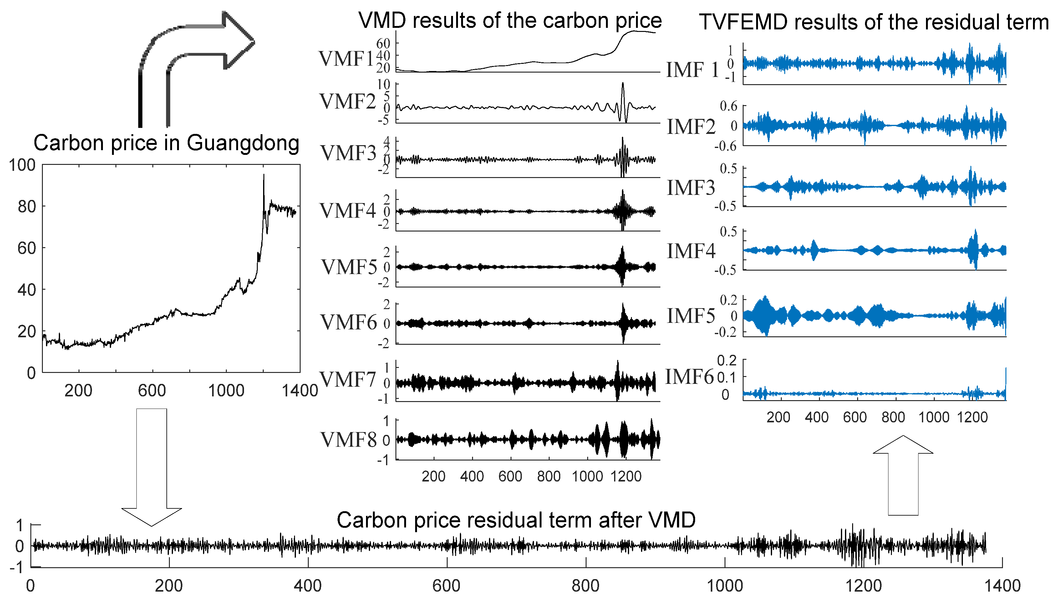
The carbon price residual term generated by VMD fluctuates violently and lacks regularity. This study utilizes TVFEMD to weaken the prediction difficulty of the residual term. Li et al. (2017) [49] proposed the TVFEMD. When compared to EMD, the TVFEMD method helps avoid mode aliasing and retain the time-varying characteristics of signals [50]. The following are the main steps of the TVFEMD algorithm:

Step 1: Perform the Hilbert transform on the raw data series S(t), and the result is noted as R(t). Then, calculate A(t) and λ(t). A(t) is the instantaneous amplitude of the S(t). λ(t) is the instantaneous phase.

$$\mathrm{A}(t)=\sqrt{S{(t)}^2+R{(t)}^2}$$

(6)

$$\lambda (t)=\arctan [S(t)/R(t)]$$

(7)

Step 2: Define the local maximum and local minimum of the A(t), recorded as A({t_max}) and A({t_min}). Then, A({t_max}) and A({t_min}) are interpolated to obtain $cu{r}_1(t)$ and $cu{r}_2(t)$. ${\gamma }_1(t)$ and ${\gamma }_2(t)$ are calculated as below.

$${\gamma }_1(t)=\frac{cu{r}_1(t)+cu{r}_2(t)}{2}$$

(8)

$${\gamma }_2(t)=\frac{cu{r}_1(t)-cu{r}_2(t)}{2}$$

(9)

Step 3: λ({t_min})A²({t_min}) and λ({t_max})A²({t_max}) are interpolated to obtain β₁(t) and β₂(t); then, calculate the instantaneous frequency component ${{\displaystyle \lambda }}_1^{\prime }(t)$, ${{\displaystyle \lambda }}_2^{\prime }(t)$.

$${{\displaystyle \lambda }}_1^{\prime }(t)=\frac{{\beta }_1(t)}{2{\gamma }_1{}^2(t)-2{\gamma }_1(t){\gamma }_2(t)}+\frac{{\beta }_2(t)}{2{\gamma }_1{}^2(t)+2{\gamma }_1(t){\gamma }_2(t)}$$

(10)

$${{\displaystyle \lambda }}_2^{\prime }(t)=\frac{{\beta }_1(t)}{2{\gamma }_2{}^2(t)-2{\gamma }_1(t){\gamma }_2(t)}+\frac{{\beta }_2(t)}{2{\gamma }_2{}^2(t)+2{\gamma }_1(t){\gamma }_2(t)}$$

(11)

Step 4: Define ${{\displaystyle \lambda }}_{\mathrm{bis}}^{\prime }(t)$, which is local cut-off frequency:

$${{\displaystyle \lambda }}_{\mathrm{bis}}^{\prime }(t)=\frac{{{\displaystyle \lambda }}_1^{\prime }(t)+{{\displaystyle \lambda }}_2^{\prime }(t)}{2}$$

(12)

Step 5: Readjust ${{\displaystyle \lambda }}_{\mathrm{bis}}^{\prime }(t)$ to solve the intermittent problem.

Step 6: Define $\phi (t)=\cos [{\displaystyle \int {\lambda }_{\mathrm{bis}}^{\prime }}(t)d(t)]$, where is employed to build the time-varying filter. B-spline interpolation is utilized to filter S(t), and the outcome of the approximation is given as m(t).

Step 7: When $\sigma (t)\le r$ is met, S(t) is determined as an IMF. Otherwise, S(t) = S(t) − m(t), repeat the previous steps.

$$\sigma (t)=\frac{B_{loughlin}(t)}{{\lambda }_{avg}(t)}$$

(13)

where $\sigma (t)$ is the stop condition, ${\lambda }_{avg}(t)$ is the weighted average of the instantaneous frequency, and $B_{loughlin}(t)$ is the Loughlin instantaneous bandwidth. The value of r is set to 0.1.

Eventually, several IMF components are acquired.

3.3. MKELM Optimized by SSA

3.3.1. Basic Theory of MKELM

As a novel feedforward neural network, ELM model has less parameter setting, a faster learning rate, stronger generalization ability, simplicity, and ease of use. However, the input weights and hidden layer thresholds of the ELM model are created randomly. Meanwhile, the number of hidden layer nodes of the ELM needs to be determined subjectively. These shortcomings will weaken its the stability. To alleviate the problem, Huang et al. (2012) [51] developed the KELM. Compared with ELM, the regression result of KELM is more stable [52]. In KELM, the kernel mapping replaces the random mapping. The generalization ability and stability of the KELM model is superior to ELM. However, different kernel functions have significantly different forecasting performance. Any base kernel may not be suitable for a variety of applications. Usually, the KELM with a single kernel function has limited representation capability and struggles to capture the complicated characteristics in carbon price. Compared with KELM, the MKELM has better generalization performance and learning ability and can enhance forecasting performance. Therefore, the MKELM is used to forecast carbon price.

For the training dataset $({{\displaystyle x}}_i,{{\displaystyle t}}_i)$, the input included in the forecasting model is ${{\displaystyle x}}_i$, and ${{\displaystyle t}}_i$ is its output. The standard KELM regression model can be displayed as follows:

$$f(x)=\left[\begin{array}{l} K(x,{{\displaystyle x}}_1)\\ ⋮\\ K(x,{{\displaystyle x}}_N)\end{array}\right]{(I/C+{\mathbf{\Omega }}_{KELM})}^{-1}\mathbf{T}$$

(14)

In Equation (14), ${\mathbf{\Omega }}_{KELM}$ is a kernel matrix, $I$ is a unit diagonal matrix, $C$ represents a regularization coefficient, the addition of C can improve stability, and $\mathbf{T}$ is the target output matrix.

The kernel function $K({{\displaystyle x,x}}_i)$ has an important influence on the prediction ability of KELM. The popular kernel functions used in the KELM model are RBF kernel, poly kernel, and wavelet kernel function. They are, respectively, expressed as $K_{\mathrm{rbf}}$, $K_{\mathrm{poly}}$, and $K_{\mathrm{wav}}$. The corresponding formulas of $K_{\mathrm{rbf}}$, $K_{\mathrm{poly}}$, and $K_{\mathrm{wav}}$ are as follows:

①

$K_{\mathrm{rbf}}(x,x_i)=\exp (-\frac{{{\displaystyle \Vert }x-x_i{\displaystyle \Vert }}^2}{a})$

②

$K_{\mathrm{poly}}(x,x_i)=(x\cdot x_i+b{)}^d$

③

$K_{\mathrm{wav}}(x,x_i)=\cos \left(\frac{g_1(x-x_i)}{g_2}\right)\exp \left(-\frac{{{\displaystyle \Vert }x-x_i{\displaystyle \Vert }}^2}{g_3}\right)$

where d is the order of the $K_{\mathrm{poly}}$. While $K_{\mathrm{poly}}$ has superior generalization capabilities, $K_{\mathrm{rbf}}$ has better learning capabilities [53], and wavelet kernel function has the advantages of wavelet signal local analysis and multi-resolution analysis [54]. Each single kernel function often has its own application field, making it challenging for them to maximize their capacity for representation. An unsuitable kernel function may have a negative impact on the predicted precision of the price of carbon [55]. It is thus crucial for modeling and prediction to build a general multiple-kernel-based function for KELM. Based on Mercer’s theory, another kernel function can be created by linearly mixing different kernel functions. To combine the advantages of $K_{\mathrm{rbf}}$, $K_{\mathrm{poly}}$, and $K_{\mathrm{wav}}$ to their fullest extent, this paper constructs the following combined kernel function, which is made up of multiple kernel functions:

$$K_{\mathrm{comb}}(x,x_i)=w_1\cdot K_{{}_{\mathrm{rbf}}}+(1-w_1-w_2)\cdot K_{{}_{\mathrm{poly}}}+w_2\cdot K_{\mathrm{wav}}$$

(15)

In Equation (15), W₁ is the weight of the corresponding RBF kernel function, W₂ represents the weight of the wavelet kernel function, and $(1-w_1-w_2)$ is the weight of the poly kernel function. MKELM uses K_comb as the kernel function. When compared to KELM, MKELM, which utilizes a weighted combination of multiple kernel functions, can enhance prediction performance [56]. MKELM is therefore utilized to forecast the price of carbon. It can be seen from Equations (14) and (15) that the stability and effectiveness of the MKELM model depend primarily on the regularization coefficient C; kernel function parameters a, b, d, g₁, g₂, and g₃; and weights W₁ and W₂ in the model. These parameters need to be optimized to achieve greater predictive performance of the carbon price.

3.3.2. Sparrow Search Algorithm

As an optimization algorithm, SSA was proposed by Xue and Shen (2020) [57]. Compared with PSO, it has faster convergence, stronger optimization ability, and stronger robustness [58]. Therefore, the aforementioned parameters of the MKELM are selected by the SSA to effectively reduce the randomness of parameter selection.

In SSA, the results of optimization are obtained by simulating sparrows foraging and anti-predatory behavior. Based on the basic idea of SSA, the sparrow population is divided into three roles: discoverer, joiner, and vigilante.

The discoverers actively look for food sources. In general, the discoverers account for 10% to 20% of the total. The formula for position iteration of the discoverers is as follows:

$${{\displaystyle x}}_{id}^{t+1}=\{\begin{array}{l}{{\displaystyle x}}_{id}^t\cdot \exp (\frac{-i}{\alpha ·T}),R_2<ST\\ {{\displaystyle x}}_{id}^t+Q\cdot L,R_2\ge ST\end{array}$$

(16)

where $T$ is the maximum iterations; i = 1,2,…,N, N is the number of sparrows; $\alpha$ and $Q$ represent random numbers; t is the current times of iterations; $L$ is a matrix whose all elements are 1, with a size of 1 × d; $ST$ $\in$ [0.5, 1] represents a safe value; and $R_2$ represents a warning value between [0, 1]. When $R_2<ST$, the search environment is safe, there are no predators, and the discoverers will broaden the search area to obtain better fitness. When $R_2\ge ST$, predators are found around the foraging location, and the population immediately adjusts the search strategy.

The joiners follow the discoverer for food. The position update formula of the joiners is as given below:

$${{\displaystyle x}}_{id}^{t+1}=\{\begin{array}{l}Q\cdot \exp (\frac{{{\displaystyle xw}}_d^t-{{\displaystyle x}}_{id}^t}{i^2}),i>\frac{n}{2}\\ {{\displaystyle xb}}_d^{t+1}+\frac{1}{D}{\displaystyle \sum _{d=1}^D(rand\{-1,1\}}\cdot \left|{{\displaystyle x}}_{id}^t-{{\displaystyle xb}}_d^{t+1}\right|),i\le \frac{n}{2}\end{array}$$

(17)

where ${{\displaystyle xb}}_d^{t+1}$ is the best position, and ${{\displaystyle xw}}_d^t$ represents the worst position.

Sparrows for early warning and reconnaissance usually occupy 10% to 20% of the entire population. These sparrows are called vigilantes. The position is updated as below:

$${{\displaystyle x}}_{id}^{t+1}=\{\begin{array}{l}{{\displaystyle xb}}_d^t+\beta ({{\displaystyle x}}_{id}^t-{{\displaystyle xb}}_d^t),f_i\ne f_g\\ {{\displaystyle x}}_d^{t+1}+K(\frac{{{\displaystyle x}}_{id}^t-{{\displaystyle xw}}_d^t}{\left|f_i-f_w\right|+e}),f_i=f_g\end{array}$$

(18)

where ${xb}_d$ is the globally optimal location, and K$\in$ [−1, 1] represents a random number. $e$ is a minimal constant for avoiding the situation in which the denominator equals 0, $f_i$ is the fitness value of the current sparrow, $f_g$ is the global optimal, and $f_w$ represents the worst fitness values. β represents a random digit obeying standard normal distribution.

All in all, the sparrow population iterates based on the Equations (16)–(18). Once the conditions are met, the process of position updating of the sparrow population ends.

3.4. Error Correction Strategy of Carbon Price Prediction

Any prediction model will have a certain degree of prediction error. Critical information for carbon price forecasting is contained in the prediction error of carbon price. Hence, it is essential to fully utilize the effective information contained in the historical forecasting error. To further strengthen the prediction performance of the carbon price, the initial prediction error can be predicted to modify the prediction of the original carbon price, thereby weakening the inherent error of the combined model. The initial prediction error of carbon price in this paper is obtained by subtracting the initial prediction value of carbon price from the original carbon price. The choice of a correction strategy for the initial prediction error is the key to carbon price-prediction error correction. The current error-correction studies frequently employ the strategy of a simple addition of the error-prediction value and the initial prediction value to arrive at the final prediction result of the carbon price. However, the simple addition strategy has some limitations in capturing the impact of the error sequence and the initial prediction on the overall prediction result of the carbon price. To tackle carbon price forecasting with more precision, a nonlinear error-correction approach is required. Accordingly, based on SSA-MKELM, this research suggests a nonlinear correction technique. The following are the steps of the error-correction technique for predicting the price of carbon:

Step 1: Create the error-prediction model to predict the error.

The initial prediction error of the carbon price is a set of time-series data. The autocorrelation of the error series is determined by PACF as the lag of the error series. Define Error(t) as the initial prediction error of the carbon price in period t. Using the historical data of Error (t) as the input term, the SSA-MKELM model is adopted to train and predict Error(t), and the predicted value of the error series in period t is obtained and recorded as EForecast(t).

EForecast(t) = MKELM(EForecast(t − 1), EForecast(t − 2),…, EForecast(t − n))

Step 2: Carry out a non-linear correction to determine the final predicted results of the carbon price.

The performance of the forecast model of the carbon price can be increased by implementing an efficient error-correction approach. In this paper, a nonlinear error-correction strategy based on SSA-MKELM is proposed; that is, take the EForecast(t) and the initial prediction value of carbon price Forecast(t) as the input item of the MKELM model, take the actual price of carbon price in t period as the output item, build the mapping relationship between the input and the actual carbon price through sample training and learning, and then obtain the final prediction. The expression is as follows:

$$\widehat{y}(t)=\mathrm{MKELM}(EForecast(t),Forecast(t))$$

3.5. The Framework of the Proposed Model

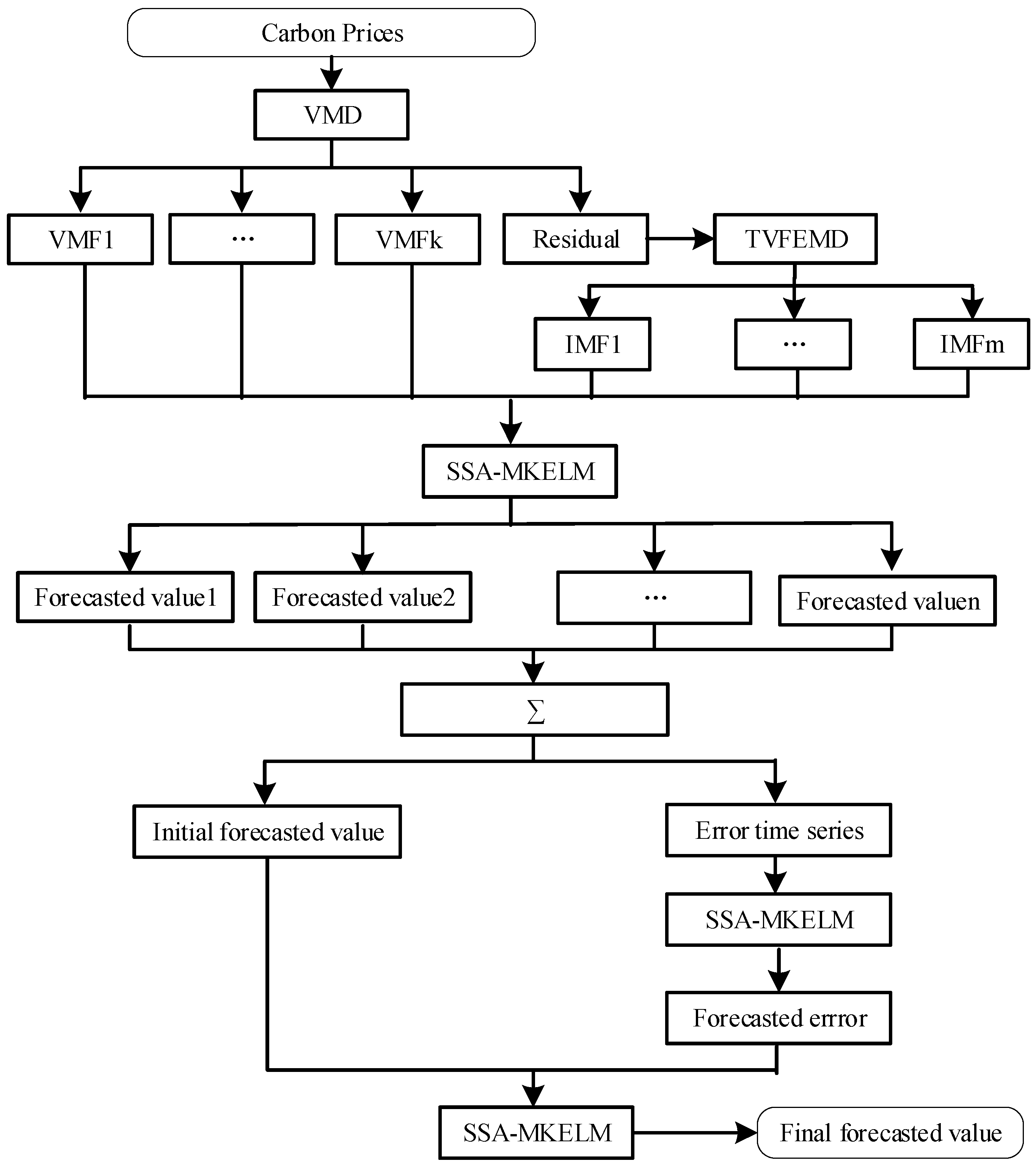
This study constructs a combined forecasting model for China’s regional carbon price based on secondary decomposition and a nonlinear error-correction strategy called the VMD-TVFEMD-SSA-MKELM-ENC model. Figure 1 is the flowchart of the model. The following are the detailed modeling steps:

(1)

Decomposition of the carbon price series: VMD is utilized to decompose the carbon price into several VMF components, which contain the main information of the carbon price. Subtract the sum of all VMF components from the carbon price to obtain a residual term. The residual term is a time series with irregular fluctuations. As an indispensable part of the carbon price, it offers valuable information for predicting the carbon price. Therefore, the residual term must be taken into account when predicting the price of carbon. The residual term is decomposed by TVFEMD to lessen its complexity. As a result, the residual term is divided into several IMFs;

(2)

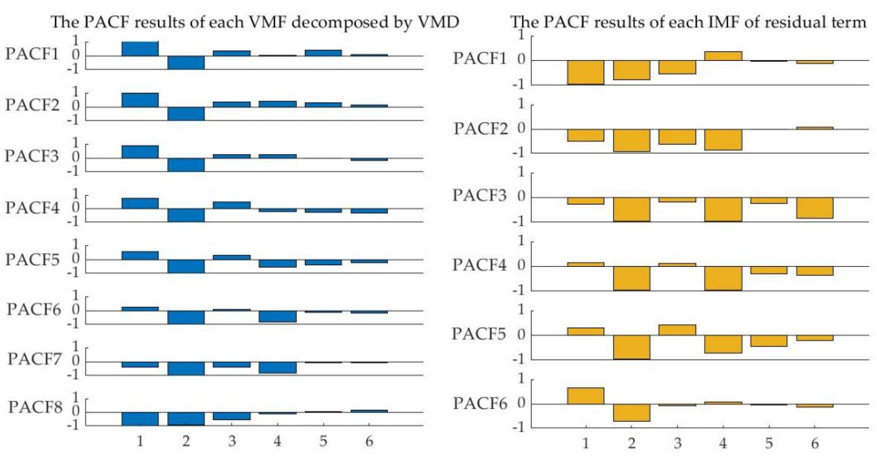
Initial prediction of the carbon price: Each subsequence, including each VMF and IMF, is predicted based on the SSA-MKELM model. The input of each subsequence of carbon price is identified by the PACF test. By adding the prediction values of each VMF and IMF, the initial prediction result for the price of carbon is obtained;

(3)

Prediction of the initial prediction error: The initial prediction error is calculated by subtracting the initial prediction of carbon prices from the actual carbon prices. The SSA-MKELM model is further utilized to forecast the initial prediction error time series. Moreover, historical error data selected by PACF serve as the input;

(4)

Integrated prediction of carbon price: The SSA-MKELM is utilized again to non-linearly integrate the initial prediction and error prediction. More specifically, the initial prediction of carbon price and the prediction value of the initial prediction error are employed as input variables of the SSA-MKELM model to produce the final prediction result for carbon price.

4. Empirical Analysis

This section includes the empirical process and analysis of predicting carbon prices.

4.1. Sample Selection and Evaluation Criteria

Among the carbon pilots in China, the cumulative trading volume and turnover of the Guangdong and Hubei carbon markets have been leading the country for a long time [59]. The trading activities of these pilots are more active, and the carbon price markets are more representative. Thus, this article selects the daily spot closing price of carbon emission quotas in these two regional carbon markets as the carbon price sample data for research. Among them, the data of carbon price in Guangdong are from the Guangzhou Carbon Emission Exchange (http://www.cnemission.cn, accessed on 21 October 2022), and the sample time range is from 3 January 2017 to 20 October 2022. The data of carbon price in Hubei are from the website of the Hubei Carbon Emission Exchange (https://www.hbets.cn, accessed on 10 November 2022), and the sample time range is from 3 January 2017 to 9 November 2022. See

Table 1. Sample Data of Carbon Price.

Markets	Stage	Datasets	Date	Size
Guangdong	Stage 1	Training set	2017.01.03–2021.09.08	1106
		Test set	2021.09.09–2022.10.20	270
	Stage 2	Training set	2021.09.09–2022.08.03	218
		Test set	2022.08.04–2022.10.20	52
Hubei	Stage 1	Training set	2017.01.03–2021.09.08	1076
		Test set	2021.09.09–2022.11.09	270
	Stage 2	Training set	2021.09.09–2022.08.22	218
		Test set	2022.08.23–2022.11.09	52

for the division of sample data sets. The ratio of each training set and each test set is about 8:2. In Table 1, stage 1 is the initial prediction stage of the carbon price, and stage 2 is the stage of error correction. The empirical model of this paper runs on MATLAB 2019b.

Table 2. Descriptive statistics.

Market	Max	Min	Mean	Std. Dev.	Skewness	Kurtosis	Jarque–Bera	p-Value
Guangdong	95.26	11.05	31.89	20.57	1.34	3.67	437.22	0.000
Hubei	61.48	11.26	29.45	10.89	0.31	2.30	48.57	0.000

displays the descriptive statistics of the sample data of carbon price.

Table 2 shows that during the sample period, the minimum carbon price is about 11 yuan. The highest carbon price in Guangdong and Hubei reached 95.26 yuan/ton and 50 yuan/ton, respectively. These data demonstrate that the regional carbon price time series fluctuates significantly. The standard deviation of the carbon price in Guangdong and Hubei is 20.57 and 10.89, respectively, indicating that the carbon price data are discrete and that the carbon price in Guangdong fluctuates more violently than in Hubei. The values of skewness, kurtosis, and Jarque–Bera indicate that the carbon prices of the two markets are not subject to normal distribution.

To comprehensively evaluate the prediction effect of this model on carbon price,

Table 3. Evaluation criteria for prediction performance of carbon price.

	Index	Formula
Forecasting accuracy	RMSE	$\mathrm{RMSE}=\sqrt{\frac{1}{N}{\displaystyle \sum _{i=1}^N{(y_i-{\stackrel{{\displaystyle ⌢}}{y}}_i)}^2}}$
	MAE	$\mathrm{MAE}=\frac{1}{N}{\displaystyle \sum _{i=1}^N\left|{{\displaystyle y}}_i-{\stackrel{{\displaystyle ⌢}}{y}}_i\right|}$
	MAPE	$\mathrm{MAPE}=\frac{1}{N}{\displaystyle \sum _{i=1}^N\left|\frac{{{\displaystyle y}}_i-{\stackrel{{\displaystyle ⌢}}{y}}_i}{{{\displaystyle y}}_i}\right|}$
Forecasting direction	DS	$\begin{array}{l}\mathrm{DS}=\frac{1}{N}{\displaystyle \sum _{i=1}^n{d}_i}\\ d_i=\{\begin{array}{l}1 , \left(\mathrm{y}\right(\mathrm{t})-\mathrm{y}(\mathrm{t}-1\left)\right)\left(\hat{\mathrm{y}}\right(\mathrm{t})-\mathrm{y}(\mathrm{t}-1\left)\right)\ge 0\\ 0 ,\left(\mathrm{y}\right(\mathrm{t})-\mathrm{y}(\mathrm{t}-1\left)\right)\left(\hat{\mathrm{y}}\right(\mathrm{t})-\mathrm{y}(\mathrm{t}-1\left)\right)\le 0\end{array}\end{array}$

gives the specific calculation formula of evaluation criteria, consisting of RMSE, MAE, MAPE, and DS. The first three indicators are used to evaluate the accuracy of the prediction level. DS is used to evaluate the accuracy of the prediction direction of the model. The larger the value, the more accurate the model in judging the trend.

To more intuitively assess the prediction accuracy, three additional metrics were added. They are the P_RMSE, P_MAE, and P_MAPE. They can serve as a way to evaluate predicted performance improvements. Among them, the RMSE₁, MAE₁, and MAPE₁, respectively, represent the corresponding metrics of the benchmark model. The RMSE₂, MAE₂, and MAPE₂, respectively, represent the corresponding metrics of the comparative model.

$${\mathrm{P}}_{\mathrm{RMSE}}=\frac{{\mathrm{RMSE}}_1-{\mathrm{RMSE}}_2}{{\mathrm{RMSE}}_1}\times 100\%$$

$${\mathrm{P}}_{\mathrm{MAE}}=\frac{{\mathrm{MAE}}_1-{\mathrm{MAE}}_2}{{\mathrm{MAE}}_1}\times 100\%$$

$${\mathrm{P}}_{\mathrm{MAPE}}=\frac{{\mathrm{MAPE}}_1-{\mathrm{MAPE}}_2}{{\mathrm{MAPE}}_1}\times 100\%$$

4.2. Process of Decomposition and Prediction of Carbon Price

Due to space limitation, we take the Guangdong carbon market price as an example to show the process of decomposition, selection of input items of each subsequence, and prediction.

4.2.1. Analysis of Decomposition of Carbon Price

Before applying VMD to the carbon price, the number K of VMF components needs to be preset. The setting of K value is related to the sufficiency of carbon price feature extraction. Regarding the setting of the K, the existing literature proposed that the number of subsequences decomposed by EEMD is used as the number of K of VMD [60,61]. Since the decomposition effect of ICEEMDAN beats EEMD, and it can also automatically decompose the appropriate number of carbon price mode components, the value of K in this paper refers to the number of ICEEMDAN. Since eight components can be obtained by decomposing the carbon price in Guangdong in the whole sample period through ICEEMDAN, K is preset as 8; that is, eight VMF components can be obtained by VMD. The residual term generated by VMD fluctuates violently and is highly complicated. To better grasp the fluctuation rule of the residual term, the TVFEMD is further employed to decompose it into six IMF components. Figure 2 displays the specific decomposition consequence of VMD-TVFEMD for the carbon price in Guangdong:

In Figure 2, the carbon prices in the Guangdong market are decomposed by VMD. Based on this, eight VMF subsequences and a residual term are obtained. Among them, eight VMF series have obvious fluctuation rules, while the residual series has intricate fluctuations and a lack of rules. The residual term is decomposed by TVFEMD, and six IMF subsequences containing residual fluctuation information are obtained. Finally, 14 subsequences are obtained. These 14 subsequences are more regular, representing the carbon price laws of different fluctuation periods, respectively.

4.2.2. Selection of Input Variables

The selection of the input is essential for forecasting these subseries of carbon prices. The PACF is a common method to determine the lag period of time series. This paper adopts the PACF to examine the autocorrelation of each subsequence of carbon price (Figure 3). In Figure 3, each subsequence of carbon price will be influenced by its own previous historical data to varying degrees.

Based on the above PACF consequences,

Table 4. Input of each subsequence prediction model.

Subseries	Lag	Subseries	Lag
VMF1	1,2,3,5	VMF8	1,2,3,4,6
VMF2	1,2,3,4,5,6	IMF1	1,2,3,4,6
VMF3	1,2,3,4,6	IMF2	1,2,3,4
VMF4	1,2,3,4,5,6	IMF3	1,2,3,4,5,6
VMF5	1,2,3,4,5,6	IMF4	1,2,3,4,5,6
VMF6	1,2,4,5,6	IMF5	1,2,3,4,5,6
VMF7	1,2,3,4	IMF6	1,2,6

details the input of the prediction models for each subsequence.

In Table 4, different subsequences may have different degrees of autocorrelation from historical data, which also indicates the necessity of the PACF test. Obviously, the forecasting models for VMF2, VMF4, VMF5, IMF3, IMF4, and IMF5 take the data from the preceding six trading days as their input.

4.2.3. Prediction Process of Carbon Price

In the first stage, the initial prediction of the carbon price is carried out. The MKELM model optimized by SSA is employed to predict each VMF and IMF component, respectively. Then, the initial prediction result for carbon price is obtained by superimposing the prediction results of each subsequence. The combined model that performs secondary decomposition and the initial prediction of carbon price is defined as the VMD-TVFEMD-SSA-MKELM model. The optimization process of SSA for each key parameter consisting of a, b, d, g₁, g₂, g₃ and w₁ and w₂ is implemented in the training phase of the MKELM model. The following are the parameter settings for the SSA: the pop is set to 20, the maximum number of iterations is set to 20, the search range of d is [1, 10], the search range for both W₁ and W₂ is [0, 1], and the search range of the other parameters = [0.001, 1000].

Table 5. The parameters of MKELM model for forecasting carbon price subsequences.

Subseries	W1	W2	C	a	b	d	g1	g2	g3
VMF1	0.2	0.1	559	169	561	2	227	61	111
VMF2	0.03	0.1	495	920	366	1	750	285	439
VMF3	0.002	0.01	711	867	118	1	598	604	516
VMF4	0.003	0.3	220	88	253	1	294	461	1
VMF5	0.04	0.1	338	430	859	1	506	618	282
VMF6	0.7	0.2	890	959	547	2	149	257	840
VMF7	0.1	0.4	712	823	705	1	675	84	574
VMF8	0.3	0.02	678	246	123	1	602	361	287
IMF1	0.32	0.71	118	39	932	2	475	598	604
IMF2	0.3	0.2	393	409	80	1	293	39	0.1
IMF3	0.2	0.3	763	914	28	1	448	654	139
IMF4	0.1	0.8	54	212	81	3	867	16	0.04
IMF5	0.8	0.1	264	212	94	2	138	746	202
IMF6	0.4	0.5	922	492	904	3	83	53	298

shows the key parameters of the MKELM model obtained through the SSA optimization algorithm.

In Table 5, the $K_{\mathrm{poly}}$ has the biggest weight for the training of VMF1–VMF5, VMF7–VMF8, and IMF2–IMF3, suggesting that this kernel function is more crucial for the prediction of these sequences. The weight of $K_{\mathrm{wav}}$ for training IMF1 and IMF4 is as high as 0.71 and 0.8, respectively, indicating that it will be more important in the prediction of these sequences. The $K_{\mathrm{rbf}}$ has the biggest weight for the training of VMF6 and IMF5, indicating that this kernel function will be more useful in the prediction of these sequences. The analysis mentioned above supports the idea that different kernel functions may be better suited for the prediction of certain subsequences. It also proves the necessity of constructing combined kernel function.

The prediction performance of each subsequence by using SSA-MEKLM is displayed in

Table 6. The prediction performance of each carbon price subsequence.

Series	RMSE	MAE	MAPE	DS
VMF1	0.0153	0.01118	0.0002	0.9593
VMF2	0.0252	0.0173	0.0876	0.9704
VMF3	0.0327	0.0226	0.6981	0.9667
VMF4	0.0392	0.0269	0.1945	0.9667
VMF5	0.0420	0.0294	0.3269	0.9852
VMF6	0.0461	0.0338	0.7043	0.9593
VMF7	0.0414	0.0295	0.5768	0.9778
VMF8	0.0140	0.0101	0.1272	0.9963
IMF1	0.0031	0.0023	0.0450	0.9926
IMF2	0.0191	0.0149	1.3208	0.9741
IMF3	0.0047	0.0034	0.1535	0.9926
IMF4	0.0040	0.0025	0.1198	0.9852
IMF5	0.0018	0.0013	0.1104	0.9926
IMF6	0.0045	0.0027	0.8796	0.8852

. It is evident that the prediction performance of the MKELM optimized by SSA for each subsequence is good. It shows that this method is suitable for forecasting each subsequence of carbon price.

To extract useful information from the historical error series more effectively and reduce the impact of system error on the prediction accuracy of the carbon price, we enter the second stage. This phase comprises two steps: error prediction and ensemble learning. Firstly, the MKELM model optimized by SSA is used to predict the error of initial prediction of carbon price, and the predicted value of the error is obtained. Then, an ensemble learning model based on SSA-MKELM is constructed, where the initial prediction results and error-prediction results of carbon price act as the input to obtain the final prediction results of carbon price. The results of parameter optimization in this stage are shown in

Table 7. Optimal parameters of MKELM model in error-correction stage.

Model	W1	W2	C	a	b	d	g1	g2	g3
Error prediction	0.70	0.60	964	0.002	132	2	652	330	977
Ensemble learning	0.34	0.70	563	147	606	1	237	39	83

. Up until now, a comprehensive process consisting of secondary decomposition, initial prediction, and error correction of the carbon price has been accomplished. That is, using these optimal parameters, the prediction of the carbon price based on the VMD-TVFEMD-SSA-MKELM-ENC model can be acquired.

4.3. Comparison and Analysis of Carbon Price Prediction Effect

4.3.1. Comparative Analysis of Initial Prediction Effect of Carbon Price

To demonstrate the effectiveness of the initial prediction model VMD-TVFEMD-SSA-MKELM, this model is compared with the reference group models. The reference group models are composed of the SSA-HKELM, SSA-MKELM, the VMD-SSA-MKELM model, and the TVFEMD-SSA-MKELM model. Among them, SSA-HKELM and SSA-MKELM are two benchmark models that exclude decomposition technique. The input of these single models for carbon price prediction is the historical data on the carbon price, which is determined by the PACF. The VMD-SSA-MKELM model is applied VMD to process carbon prices, disregarding the residual term, and then, we utilize the SSA-MKELM to predict each subseries before aggregating the predictions of each subseries. The TVFEMD-SSA-MKELM model applies TVFEMD to decompose the carbon price and then employs SSA-MKELM to forecast each subseries before adding up the predictions of all subsequences. The VMD-SSA-MKELM and the TVFEMD-SSA-MKELM are single decomposition-based models. Figure 4 displays the initial predictions of the above models on the carbon price in Guangdong and Hubei.

Table 8. Comparison of initial predictive performance of carbon price.

Dataset	Models	RMSE	MAE	MAPE	DS
	SSA-HKELM	1.5865	0.9488	0.0139	0.5556
	SSA-MKELM	1.5744	0.9365	0.0138	0.5667
Guangdong	VMD-SSA-MKELM	0.2149	0.1591	0.0024	0.9296
	TVFEMD-SSA-MKELM	0.2377	0.1630	0.0024	0.9000
	VMD-TVFEMD-SSA-MKELM	0.1639	0.1219	0.0019	0.9333
	SSA-HKELM	1.0934	0.6130	0.0140	0.5000
	SSA-MKELM	1.0897	0.5960	0.0136	0.5481
Hubei	VMD-SSA-MKELM	0.2845	0.2043	0.0047	0.8222
	TVFEMD-SSA-MKELM	0.2543	0.1785	0.0042	0.8481
	VMD-TVFEMD-SSA-MKELM	0.1245	0.0888	0.0020	0.9074

shows the comparison of the prediction performance, and

Table 9. The improvement percentage of the models.

Dataset	Benchmark Model	Comparative Model	PRMSE	PMAE	PMAPE
	SSA-HKELM	SSA-MKELM	0.76%	1.30%	0.72%
Guangdong	SSA-MKELM	VMD-SSA-MKELM	86.35%	83.01%	82.61%
	VMD-SSA-MKELM	VMD-TVFEMD-SSA-MKELM	23.73%	23.38%	20.83%
	TVFEMD-SSA-MKELM	VMD-TVFEMD-SSA-MKELM	31.05%	25.21%	20.83%
	SSA-HKELM	SSA-MKELM	0.34%	2.77%	2.86%
Hubei	SSA-MKELM	VMD-SSA-MKELM	73.89%	65.72%	65.44%
	VMD-SSA-MKELM	VMD-TVFEMD-SSA-MKELM	56.24%	56.53%	57.45%
	TVFEMD-SSA-MKELM	VMD-TVFEMD-SSA-MKELM	51.04%	50.25%	52.38%

shows the improvement percentage of the different forecasting models.

Table 8 quantifies the forecasting performance of the models and suggests the following points:

In terms of the Guangdong market, the specific comparative analysis is as follows: (1) Each evaluation criterion demonstrates that VMD-TVFEMD-SSA-MKELM model out-performs the reference group models. The RMSE, MAE, MAPE, and DS of the VMD-TVFEMD-SSA-MKELM are the best of all models. Their values are 0.1639, 0.1219, 0.0019, and 0.9333, respectively. (2) In terms of the comparison among single models, compared with the SSA-HKELM model, the SSA-MKELM model shows superior predictive capacity. The values of RMSE, MAE, and MAPE of the SSA-HKELM are larger than those of SSA-MKELM. The DS of the SSA-HKELM is lower than that of the SSA-MKELM. This is primarily because the weighted kernel function adopted by MKELM is more flexible, and the addition of wavelet kernel function to MKELM can improve the forecasted performance of the carbon price to a certain extent. Thus, the MKELM is a more promising approach. (3) The prediction capability of the hybrid models outperforms that of the single models. For instance, compared with SSA-MKELM model, the VMD-SSA-MKELM obtains a lower RMSE value of 0.2149. This is because the combined model weakens the complexity of the carbon price series through signal decomposition technology. (4) The model using the secondary decomposition of VMD-TVFEMD is superior to the model using the single decomposition. For instance, comparison between VMD-SSA-MKELM and VMD-TVFEMD-SSA-MKELM reveals that the latter performs better, with a lower RMSE of 0.1639. This is because the introduction of TVFEMD to decompose the residual sequence generated by VMD can improve the decomposition effect, which verifies the decomposition effectiveness of the combination of VMD and TVFEMD.

In terms of the Hubei market, we next compare the results of the VMD-TVFEMD-SSA-MKELM model and the reference group. They show tendencies and conclusions similar to those drawn for the Guangdong market. As expected, the VMD-TVFEMD-SSA-MKELM model achieves the optimal RMSE, MAE, MAPE, and DS of 0.1245, 0.0888, 0.0020, and 0.9074, respectively. It confirms the forecasting effectiveness of the model.

Table 9 investigates the contributions to improvement further. It suggests the following points:

In the Guangdong market, the following can be seen: (1) In these single models, the SSA-MKELM is better. Compared with the SSA-HKELM, the RMSE, MAE, and MAPE of the SSA-MKELM model are improved by 0.76%, 1.30%, and 0.72%, respectively. (2) Comparing the SSA-MKELM with the VMD-SSA-MKELM, the three indicators of this model are improved by 86.35%, 83.01%, and 82.61%, respectively. (3) The three indicators of the VMD-TVFEMD-SSA-MKELM model improved by 31.05%, 25.21%, and 20.83% when it is in contrast with TVFEMD-SSA-MKELM. These results well support those in Table 8.

The relative values of the P_RMSE, P_MAE, and P_MAPE on the Hubei market did not differ considerably from the findings on the Guangdong market.

4.3.2. Comparative Analysis of Error-Correction Effect

To further verify the feasibility of the error nonlinear correction strategy proposed in this paper, this part compares the model without error correction (VMD-TVFEMD-SSA-MKELM), the direct error-correction model (VMD-TVFEMD-SSA-MKELM-EC), and the error nonlinear correction model (VMD-TVFEMD-SSA-MKELM-ENC). More specifically, the direct error-correction strategy means that the final prediction result is obtained by directly adding the error-prediction value and the initial prediction value of the original model. See Figure 5 and Figure 6 and

Table 10. Comparison of error-correction prediction performance of carbon price.

Dataset	Models	RMSE	MAE	MAPE	DS
Guangdong	VMD-TVFEMD-SSA-MKELM	0.1501	0.1268	0.0016	0.9231
	VMD-TVFEMD-SSA-MKELM-EC	0.1410	0.1166	0.0015	0.9231
	VMD-TVFEMD-SSA-MKELM-ENC	0.1363	0.1160	0.0015	0.9231
Hubei	VMD-TVFEMD-SSA-MKELM	0.0580	0.0479	0.0009	0.8654
	VMD-TVFEMD-SSA-MKELM-EC	0.0527	0.0418	0.0008	0.9231
	VMD-TVFEMD-SSA-MKELM-ENC	0.0523	0.0408	0.0008	0.9231

for the comparison of prediction results and prediction performance for different models in the stage of error correction.

Table 11. The improvement percentage.

Dataset	Benchmark Model	Comparative Model	PRMSE	PMAE	PMAPE
Guangdong	VMD-TVFEMD-SSA-MKELM	VMD-TVFEMD-SSA-MKELM-EC	6.06%	8.04%	6.25%
	VMD-TVFEMD-SSA-MKELM-EC	VMD-TVFEMD-SSA-MKELM-ENC	3.33%	0.51%	0.00%
	VMD-TVFEMD-SSA-MKELM	VMD-TVFEMD-SSA-MKELM-ENC	9.19%	8.52%	6.25%
Hubei	VMD-TVFEMD-SSA-MKELM	VMD-TVFEMD-SSA-MKELM-EC	9.14%	12.73%	11.11%
	VMD-TVFEMD-SSA-MKELM-EC	VMD-TVFEMD-SSA-MKELM-ENC	0.76%	2.39%	0.00%
	VMD-TVFEMD-SSA-MKELM	VMD-TVFEMD-SSA-MKELM-ENC	9.83%	14.82%	11.11%

displays the improvement percentage of the proposed model in the Guangdong and Hubei markets.

Figure 5 intuitively reveals that the predicted value of carbon price in both markets after nonlinear error correction has a high consistency with the true value of carbon price, demonstrating the practicability of the VMD-TVFEMD-SSA-MKELM-ENC model. Moreover, by deducting the predicted value from the actual carbon price, the prediction error in the ordinate of Figure 6 is obtained. Figure 6 illustrates that the prediction errors of the proposed model are lower than those of other models.

In Table 10 and Table 11, the VMD-TVFEMD-SSA-MKELM-ENC model outperforms other considered models. The prediction effect of the model can be further assessed:

In terms of the Guangdong market, from the perspective of predictive performance, the following can be seen: (1) The nonlinear error-correction strategy outperforms the linear correction strategy. The VMD-TVFEMD-SSA-MKELM-ENC model achieves the optimal RMSE, MAE, MAPE, and DS of 0.1363, 0.1160, 0.0015, and 0.9231, respectively. That is, the performance of the VMD-TVFEMD-SSA-MKELM-ENC model is superior to the VMD-TVFEMD-SSA-MKELM-EC model. The reason for this could be that the direct superposition correction strategy is a linear correction strategy that ignores the importance of potential nonlinear relationships in improving the prediction performance of the model, whereas the initial prediction value of carbon price and the error-prediction value may have different importance to the overall carbon price. (2) The effect of the model with error-correction strategy outperforms that of the model without error correction. The RMSE, MAE, and MAPE of the VMD-TVFEMD-SSA-MKELM model are 0.1501, 0.1268, and 0.0016, respectively. For the VMD-TVFEMD-SSA-MKELM-ENC model, the three values are 0.1363, 0.1160, and 0.0015, respectively. This is due to the fact that the initial prediction error of carbon price contains more crucial information for carbon price prediction. The prediction of the initial prediction error of carbon price further enhances the prediction effect of carbon price. From the perspective of improvement contribution, (1) compared with the VMD-TVFEMD-SSA-MKELM model, the RMSE, MAE, and MAPE of the VMD-TVFEMD-SSA-MKELM-ENC model are improved by 9.19%, 8.52%, and 6.25%, respectively. (2) Compared with the VMD-TVFEMD-SSA-MKELM-EC model, the RMSE and MAE of the VMD-TVFEMD-SSA-MKELM-ENC model are improved by 3.33% and 0.51%, respectively.

In terms of the Hubei market, the relative values of these indicators did not change considerably from the findings on the Guangdong market.

As a result, it is clear that the nonlinear correction strategy is a potential method for error correction. It can be stated that the VMD-TVFEMD-SSA-MKELM-ENC is an effective and reliable prediction method.

In a word, the prediction performance of the proposed model is superior to that of the reference group models and has the validity of carbon price prediction.

5. Conclusions

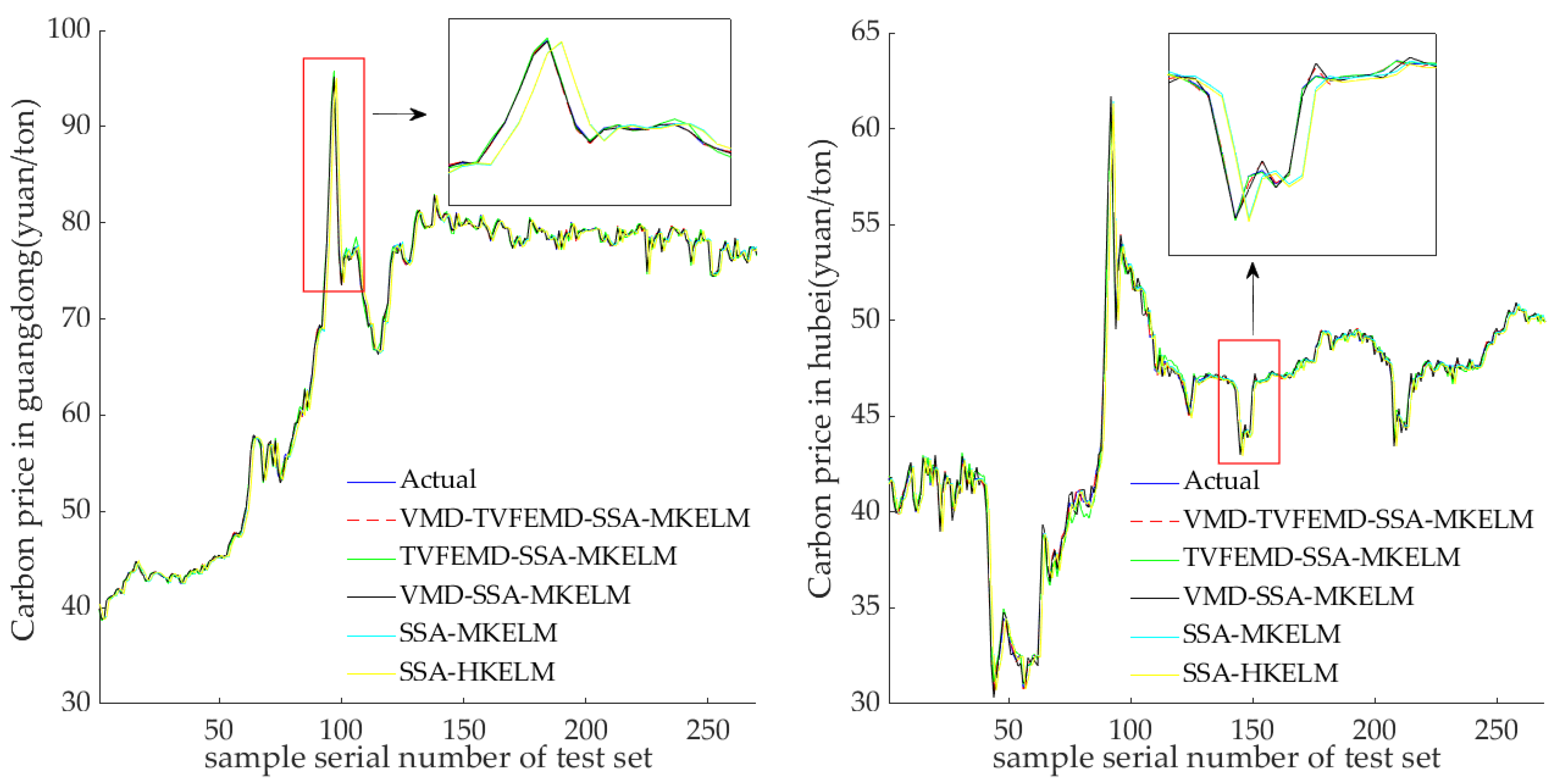
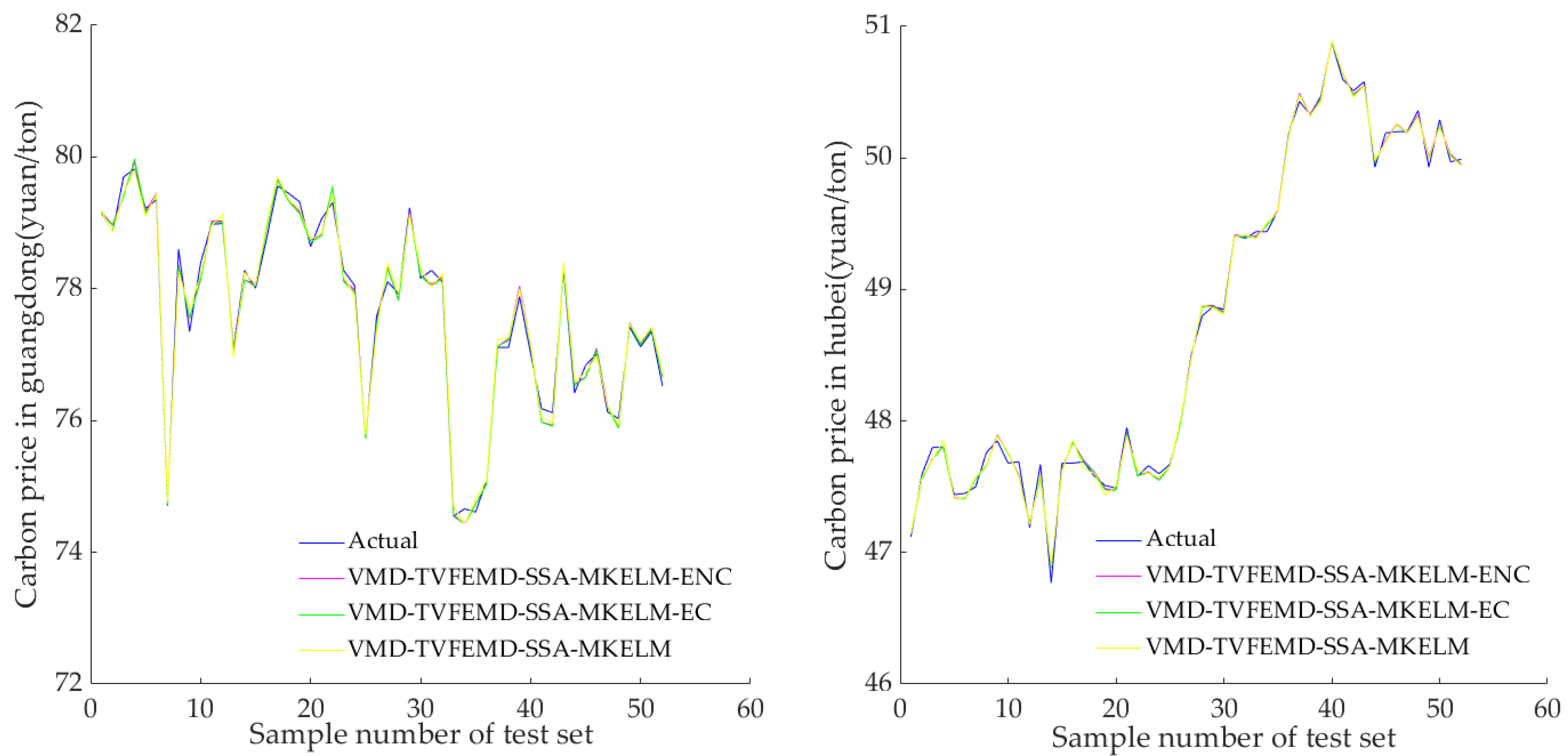
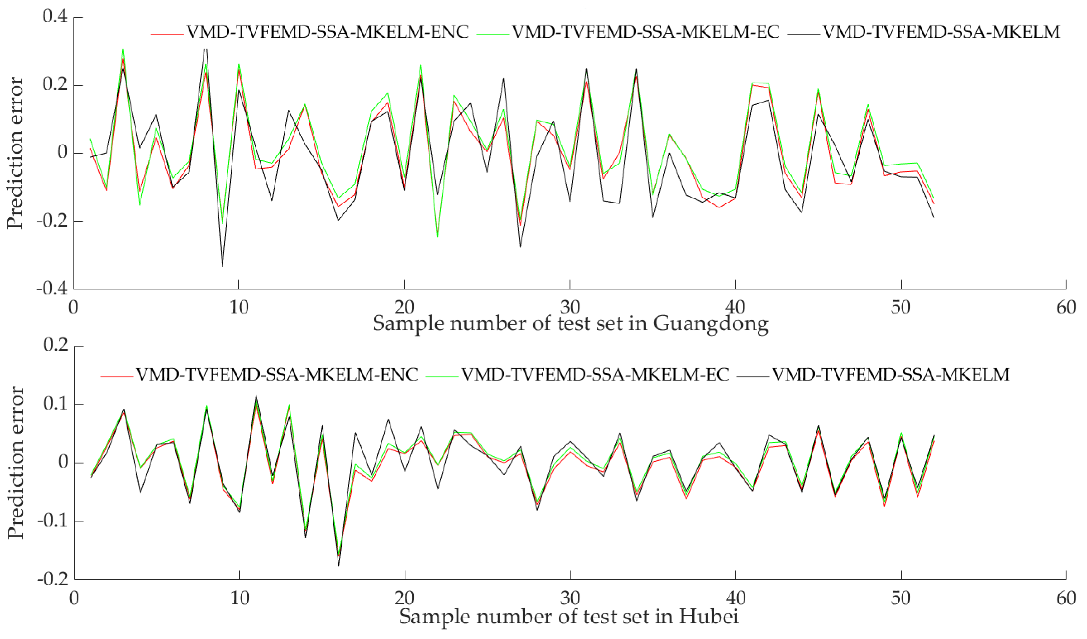
Carbon price prediction is among the crucial aspects of carbon financial market research. To address the problem in which previous studies on China’s regional carbon price forecasting based on secondary decomposition have ignored the effect of forecasting errors and only utilized HKELM models to capture the complex characteristics of regional carbon prices, the VMD-TVFEMD-SSA-MKELM-ENC model was created in this study to forecast the carbon prices in the marketplaces of Guangdong and Hubei. Firstly, the carbon prices were processed into several relatively smooth subsequences by the secondary decomposition process combining VMD and TVFEMD. Secondly, the SSA-MKELM model was constructed to forecast these subsequences of carbon price. The prediction results of these subsequences were added together to obtain the initial prediction value of the carbon price. Last but not least, a two-step nonlinear error-correction strategy was constructed to further enhance the prediction effect of the carbon price. The SSA-MKELM model was utilized to predict the initial prediction error of carbon price and was employed to nonlinearly integrate the initial prediction value and error-prediction value of carbon price to obtain the final prediction result of carbon price. The empirical results demonstrate that the proposed VMD-TVFEMD-SSA-MKELM-ENC model has superior prediction performance compared to the reference group models and that it is valid for predicting carbon prices.

The prediction model developed in this work boasts a few advantages over the existing prediction models of regional carbon prices in China: (1) The secondary decomposition method using the combination of VMD and TVFEMD can deeply explore the fluctuation characteristics and internal laws of different frequency series of carbon price, which is a feasible and effective carbon price decomposition processing method. (2) The MKELM model, which contains the multiple kernel function, is introduced to forecast the carbon price, which further improves the prediction accuracy. (3) The nonlinear error-correction strategy is innovatively introduced to correct the initial prediction results of the carbon price, which can distinguish the impact of the error series as well as the initial prediction results on the overall prediction results.

As a policy suggestion, the regional carbon prices are mainly affected by their own historical time series according to our analysis. The government can further improve the carbon price-management mechanism to avoid the risk caused by the drastic price fluctuations. Furthermore, China’s carbon market is still dominated by spot trading. Futures and options cannot be realized in these markets. Since diversified carbon financial trading tools can provide a more accurate price mechanism for carbon emissions trading, it is necessary to enrich carbon financial trading tools.

However, there are still some limitations in this study. Firstly, this analysis does not take into account how external influences may affect the price of carbon. Future work may attempt to incorporate external factors associated with the carbon price into the model to further enhance the prediction performance. Secondly, from the perspective of the optimization algorithm, the proposed prediction model only adopts single-objective optimization, and multi-objective optimization can be introduced into the proposed model in subsequent research. Finally, only the data from Guangdong and Hubei are considered, and the carbon prices of other pilots in China can be considered in the subsequent research.

References

1. Yang, L.; Hamori, S. The role of the carbon market in relation to the cryptocurrency market: Only diversification or more? Int. Rev. Financ. Anal. 2021, 77, 101864. [Google Scholar] [CrossRef]
2. Zhang, W.; Wu, Z.; Zeng, X.; Zhu, C. An ensemble dynamic self-learning model for multiscale carbon price forecasting. Energy 2023, 263, 125820. [Google Scholar] [CrossRef]
3. Wu, Q.; Wang, Y. How does carbon emission price stimulate enterprises’ total factor productivity? Insights from China’s emission trading scheme pilots. Energy Econ. 2022, 109, 105990. [Google Scholar] [CrossRef]
4. Yang, L. Idiosyncratic information spillover and connectedness network between the electricity and carbon markets in Europe. J. Commod. Mark. 2022, 25, 100185. [Google Scholar] [CrossRef]
5. Liu, M.; Yang, X.; Wen, J.; Wang, H.; Feng, Y.; Lu, J.; Chen, H.; Wu, J.; Wang, J. Drivers of China’s carbon dioxide emissions: Based on the combination model of structural decomposition analysis and input-output subsystem method. Environ. Impact Assess. Rev. 2023, 100, 107043. [Google Scholar] [CrossRef]
6. Liu, B.; Sun, Z.; Li, H. Can Carbon Trading Policies Promote Regional Green Innovation Efficiency? Empirical Data from Pilot Regions in China. Sustainability 2021, 13, 2891. [Google Scholar] [CrossRef]
7. Huang, W.; Wang, Q.; Li, H.; Fan, H.; Qian, Y.; Klemeš, J. Review of recent progress of emission trading policy in China. J. Clean. Prod. 2022, 349, 131480. [Google Scholar] [CrossRef]
8. Yuan, N.; Yang, L. Asymmetric risk spillover between financial market uncertainty and the carbon market: A GAS–DCS–copula approach. J. Clean. Prod. 2020, 259, 120750. [Google Scholar] [CrossRef]
9. Qi, S.; Cheng, S.; Tan, X.; Feng, S.; Zhou, Q. Predicting China’s carbon price based on a multi-scale integrated model. Appl. Energy 2022, 324, 119784. [Google Scholar] [CrossRef]
10. Azzaq, A.; Sharif, A.; An, H.; Aloui, C. Testing the directional predictability between carbon trading and sectoral stocks in China: New insights using cross-quantilogram and rolling window causality approaches. Technol. Forecast. Soc. Chang. 2022, 182, 121. [Google Scholar]
11. Ren, C.; Lo, A.Y. Emission trading and carbon market performance in Shenzhen, China. Appl. Energy 2017, 193, 414–425. [Google Scholar]
12. Zeng, S.; Nan, X.; Liu, C.; Chen, J. The response of the Beijing carbon emissions allowance price (BJC) to macroeconomic and energy price indices. Energy Policy 2017, 106, 111–121. [Google Scholar] [CrossRef]
13. Zhang, Y.; Liu, Z.; Xu, Y. Carbon price volatility: The case of China. PLoS ONE 2018, 13, e0205317. [Google Scholar] [CrossRef]
14. Song, Y.; Liu, T.; Liang, D.; Li, Y.; Song, X. A Fuzzy Stochastic Model for Carbon Price Prediction Under the Effect of Demand-related Policy in China’s Carbon Market. Ecol. Econ. 2019, 157, 253–265. [Google Scholar] [CrossRef]
15. Huang, Y.; Hu, J.; Liu, H.; Liu, S. Research on price forecasting method of China’s carbon trading market based on PSO-RBF algorithm. Syst. Sci. Control Eng. 2019, 7, 40–47. [Google Scholar] [CrossRef]
16. Xie, Q.; Hao, J.; Li, J.; Zheng, X. Carbon price prediction considering climate change: A text-based framework. Econ. Anal. Policy 2022, 74, 382–401. [Google Scholar] [CrossRef]
17. Liu, J.; Wang, P.; Chen, H.; Zhu, J. A combination forecasting model based on hybrid interval multi-scale decomposition: Application to interval-valued carbon price forecasting. Expert Syst. Appl. 2022, 191, 116267. [Google Scholar] [CrossRef]
18. Fan, J.; Todorova, N. Dynamics of China’s carbon prices in the pilot trading phase. Appl. Energy 2017, 208, 1452–1467. [Google Scholar] [CrossRef]
19. Wang, P.; Tao, Z.; Liu, J.; Chen, H. Improving the forecasting accuracy of interval-valued carbon price from a novel multi-scale framework with outliers detection: An improved interval-valued time series analysis mode. Energy Econ. 2023, 118, 106502. [Google Scholar] [CrossRef]
20. Han, M.; Ding, L.; Zhao, X.; Kang, W. Forecasting carbon prices in the Shenzhen market, China: The role of mixed-frequency factors. Energy 2019, 171, 69–76. [Google Scholar] [CrossRef]
21. Zhu, B. A novel multiscale ensemble carbon price prediction model integrating empirical mode decomposition, genetic algorithm and artificial neural network. Energies 2012, 5, 355–370. [Google Scholar] [CrossRef]
22. Zhang, C.; Yang, X. Forecasting of China’s regional carbon market price based on multi-frequency combined model. Syst. Eng.-Theory Pract. 2016, 36, 3017–3025. [Google Scholar]
23. Li, W.; Lu, C. The research on setting a unified interval of carbon price benchmark in the national carbon trading market of China. Appl. Energy 2015, 155, 728–739. [Google Scholar] [CrossRef]
24. Yao, Y.; Lv, J.; Zhang, C. Price formation mechanism and price forecast of Hubei carbon market. Stat. Decis. 2017, 19, 166–169. [Google Scholar]
25. Sun, W.; Xu, C. Carbon price prediction based on modified wavelet least square support vector machine. Sci. Total Environ. 2021, 754, 142052. [Google Scholar] [CrossRef] [PubMed]
26. Liang, Y.; Lin, Y.; Lu, Q. Forecasting gold price using a novel hybrid model with ICEEMDAN and LSTM-CNN-CBAM. Expert Syst. Appl. 2022, 206, 117847. [Google Scholar] [CrossRef]
27. Yang, M.; Zhu, S.; Li, W. Carbon price prediction based on multi-factor MEEMD-LSTM model. Heliyon 2022, 8, e12562. [Google Scholar] [CrossRef]
28. Wang, J.; Sun, X.; Cheng, Q.; Cui, Q. An innovative random forest-based nonlinear ensemble paradigm of improved feature extraction and deep learning for carbon price forecasting. Sci. Total Environ. 2021, 762, 143099. [Google Scholar] [CrossRef] [PubMed]
29. Wang, J.; Wang, Y.; Li, H.; Yang, H.; Li, Z. Ensemble forecasting system based on decomposition-selection-optimization for point and interval carbon price prediction. Appl. Math. Model. 2023, 113, 262–286. [Google Scholar] [CrossRef]
30. Li, D.; Li, Y.; Wang, C.; Chen, M.; Wu, Q. Forecasting carbon prices based on real-time decomposition and causal temporal convolutional networks. Appl. Energy 2023, 331, 120452. [Google Scholar] [CrossRef]
31. Sun, W.; Zhang, J. A novel carbon price prediction model based on optimized least square support vector machine combining characteristic-scale decomposition and phase space reconstruction. Energy 2022, 253, 124167. [Google Scholar] [CrossRef]
32. Zhou, J.; Chen, D. Carbon Price forecasting based on improved CEEMDAN and extreme learning machine optimized by sparrow search algorithm. Sustainability 2021, 13, 4896. [Google Scholar] [CrossRef]
33. Hao, Y.; Tian, C. A hybrid framework for carbon trading price forecasting: The role of multiple influence factor. J. Clean. Prod. 2020, 262, 120378. [Google Scholar] [CrossRef]
34. Sun, S.; Jin, F.; Li, H.; Li, Y. A new hybrid optimization ensemble learning approach for carbon price forecasting. Appl. Math. Model. 2021, 97, 182–205. [Google Scholar] [CrossRef]
35. Li, G.; Zheng, C.; Yang, H. Carbon price combination prediction model based on improved variational mode decomposition. Energy Rep. 2022, 8, 1644–1664. [Google Scholar] [CrossRef]
36. Niu, X.; Wang, J.; Zhang, L. Carbon price forecasting system based on error correction and divide-conquer strategies. Appl. Soft Comput. 2022, 118, 107935. [Google Scholar] [CrossRef]
37. Li, H.; Jin, F.; Sun, S.; Li, Y. A new secondary decomposition ensemble learning approach for carbon price forecasting. Knowl.-Based Syst. 2021, 214, 106686. [Google Scholar] [CrossRef]
38. Sun, W.; Huang, C. A carbon price prediction model based on secondary decomposition algorithm and optimized back propagation neural network. J. Clean. Prod. 2020, 243, 118671. [Google Scholar] [CrossRef]
39. Zhou, J.; Wang, S. A carbon price prediction model based on the secondary decomposition algorithm and influencing factors. Energies 2021, 14, 1328. [Google Scholar] [CrossRef]
40. Zhou, F.; Huang, Z.; Zhang, C. Carbon price forecasting based on CEEMDAN and LSTM. Appl. Energy 2022, 311, 118601. [Google Scholar] [CrossRef]
41. Li, G.; Ning, Z.; Yang, H.; Gao, L. A new carbon price prediction model. Energy 2022, 239, 122324. [Google Scholar] [CrossRef]
42. Cheng, Y.; Hu, B. Forecasting Regional Carbon Prices in China Based on Secondary Decomposition and a Hybrid Kernel-Based Extreme Learning Machine. Energies 2022, 15, 3562. [Google Scholar] [CrossRef]
43. Wu, K.; Zhu, J.; Xu, M.; Yang, L. Can crude oil drive the co-movement in the international stock market? Evidence from partial wavelet coherence analysis. N. Am. J. Econ. Financ. 2020, 53, 101194. [Google Scholar] [CrossRef]
44. Yu, M.; Niu, D.; Gao, T.; Wang, K.; Sun, L.; Li, M.; Xu, X. A novel framework for ultra-short-term interval wind power prediction based on RF-WOA-VMD and BiGRU optimized by the attention mechanism. Energy 2023, 269, 126738. [Google Scholar] [CrossRef]
45. Chen, X.; Yang, Y.; Cui, Z.; Shen, J. Vibration fault diagnosis of wind turbines based on variational mode decomposition and energy entropy. Energy 2019, 174, 1100–1109. [Google Scholar] [CrossRef]
46. Dragomiretskiy, K.; Zosso, D. Variational Mode Decomposition. IEEE Trans. Signal Process. 2014, 62, 531–544. [Google Scholar] [CrossRef]
47. Wang, Y.; Wei, Z.; Yang, J. Feature Trend Extraction and Adaptive Density Peaks Search for Intelligent Fault Diagnosis of Machines. IEEE Trans. Ind. Inform. 2019, 15, 105–115. [Google Scholar] [CrossRef]
48. Zhao, X.; Wu, P.; Yin, X. A quadratic penalty item optimal variational mode decomposition method based on single-objective salp swarm algorithm. Mech. Syst. Signal Proc. 2020, 138, 106567. [Google Scholar] [CrossRef]
49. Li, H.; Li, Z.; Mo, W. A time varying filter approach for empirical mode decomposition. Signal Process. 2017, 138, 146–158. [Google Scholar] [CrossRef]
50. Zhang, C.; Ma, H.; Hua, L.; Sun, W.; Nazir, M.; Peng, T. An evolutionary deep learning model based on TVFEMD, improved sine cosine algorithm, CNN and BiLSTM for wind speed prediction. Energy 2022, 254, 124250. [Google Scholar] [CrossRef]
51. Huang, G.; Zhou, H.; Ding, X.; Zhang, R. Extreme learning machine for regression and multiclass classification. IEEE Trans. Syst. Man Cybern. Part B-Cybern. 2012, 42, 513–529. [Google Scholar] [CrossRef] [PubMed]
52. Fu, W.; Wang, K.; Tan, W.; Zhang, K. A composite framework coupling multiple feature selection, compound prediction models and novel hybrid swarm optimizer-based synchronization optimization strategy for multi-step ahead short-term wind speed forecasting. Energy Conv. Manag. 2020, 205, 112461. [Google Scholar] [CrossRef]
53. Lv, L.; Wang, W.; Zhang, Z.; Liu, X. A novel intrusion detection system based on an optimal hybrid kernel extreme learning machine. Knowl.-Based Syst. 2020, 195, 105648. [Google Scholar]
54. Dong, L.; Liao, J. Wavelet kernel function based multiscale LSSVM for elliptic boundary value problems. Neurocomputing 2019, 356, 40–51. [Google Scholar] [CrossRef]
55. Zhu, B.; Ye, S.; Wang, P.; He, K.; Zhang, T.; Wei, Y. A novel multiscale nonlinear ensemble leaning paradigm for carbon price forecasting. Energy Econ. 2018, 70, 143–157. [Google Scholar] [CrossRef]
56. Xie, Z.; Wu, Z. Maximum power point tracking algorithm of PV system based on irradiance estimation and multi-Kernel extreme learning machine. Sustain. Energy Technol. Assess. 2021, 44, 101090. [Google Scholar]
57. Xue, J.K.; Shen, B. A novel swarm intelligence optimization approach: Sparrow search algorithm. Sys. Sci. Control Eng. 2020, 8, 22–34. [Google Scholar] [CrossRef]
58. Li, J.; Lei, Y.; Yang, S. Mid-long term load forecasting model based on support vector machine optimized by improved sparrow search algorithm. Energy Rep. 2022, 8, 491–497. [Google Scholar]
59. Wu, Q. Price and scale effects of China’s carbon emission trading system pilots on emission reduction. J. Environ. Manag. 2022, 314, 115054. [Google Scholar] [CrossRef]
60. Li, J.; Wu, Q.; Tian, Y.; Fan, L. Monthly Henry Hub natural gas spot prices forecasting using variational mode decomposition and deep belief network. Energy 2021, 227, 120478. [Google Scholar]
61. Li, T.; Qian, Z.; Deng, W.; Zhang, D.; Lu, H.; Wang, S. Forecasting crude oil prices based on variational mode decomposition and random sparse Bayesian learning. Appl. Soft Comput. 2021, 113, 108032. [Google Scholar] [CrossRef]
Figure 1. The flowchart of the VMD-TVFEMD-SSA-MKELM-ENC model.
Energies 16 04444 g001
Figure 2. The decomposition consequence using VMD−TVFEMD.
Energies 16 04444 g002
Figure 3. The results of PACF test of the carbon price subsequences.
Energies 16 04444 g003
Figure 4. Comparison of initial predictions of carbon price.
Energies 16 04444 g004
Figure 5. Comparison of error-correction prediction results of carbon price.
Energies 16 04444 g005
Figure 6. Comparison of prediction error of carbon price.
Energies 16 04444 g006