
Maximum Power Point Tracking of Photovoltaic Module Arrays Based on a Modified Gray Wolf Optimization Algorithm


Abstract
:1. Introduction
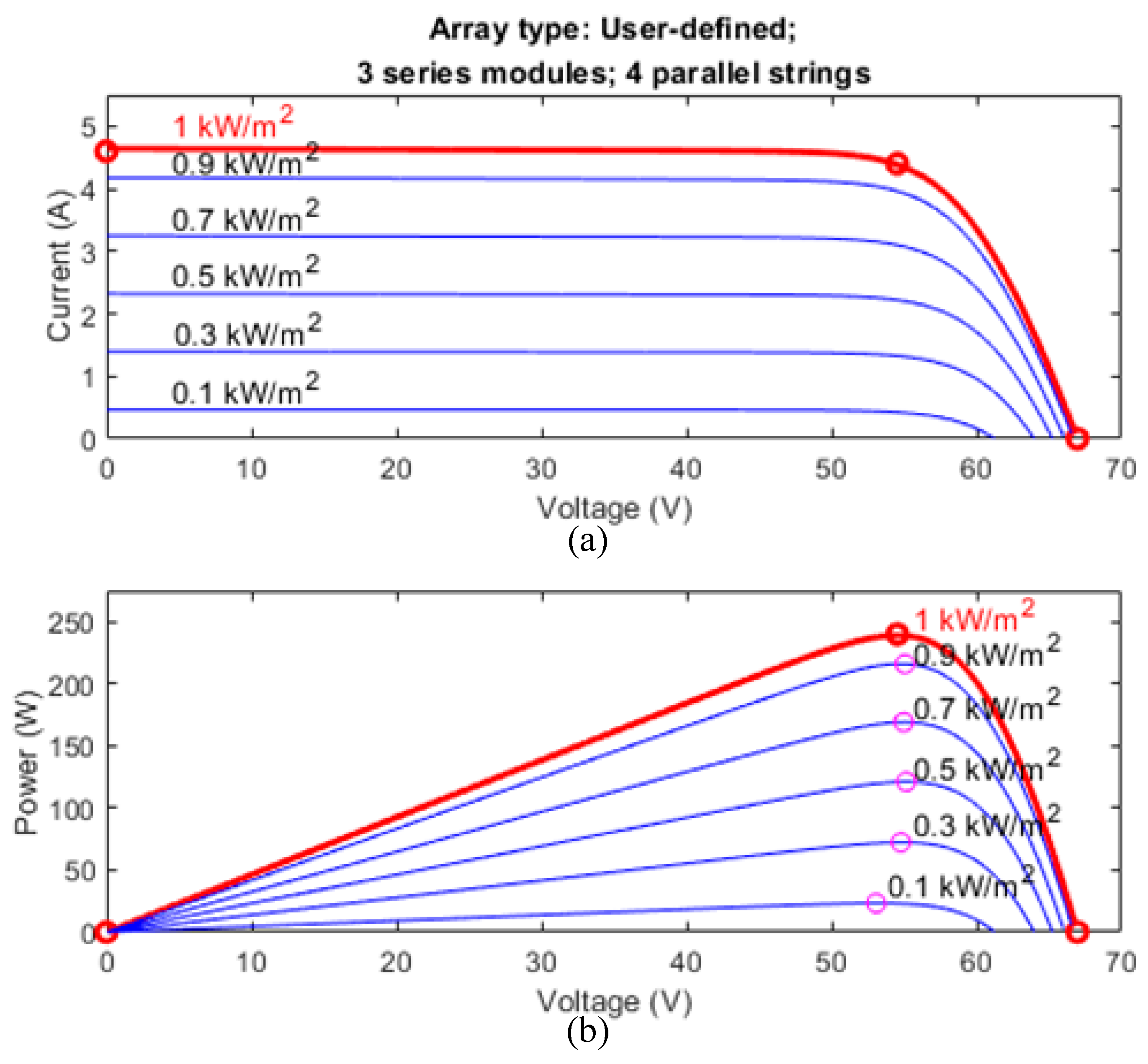
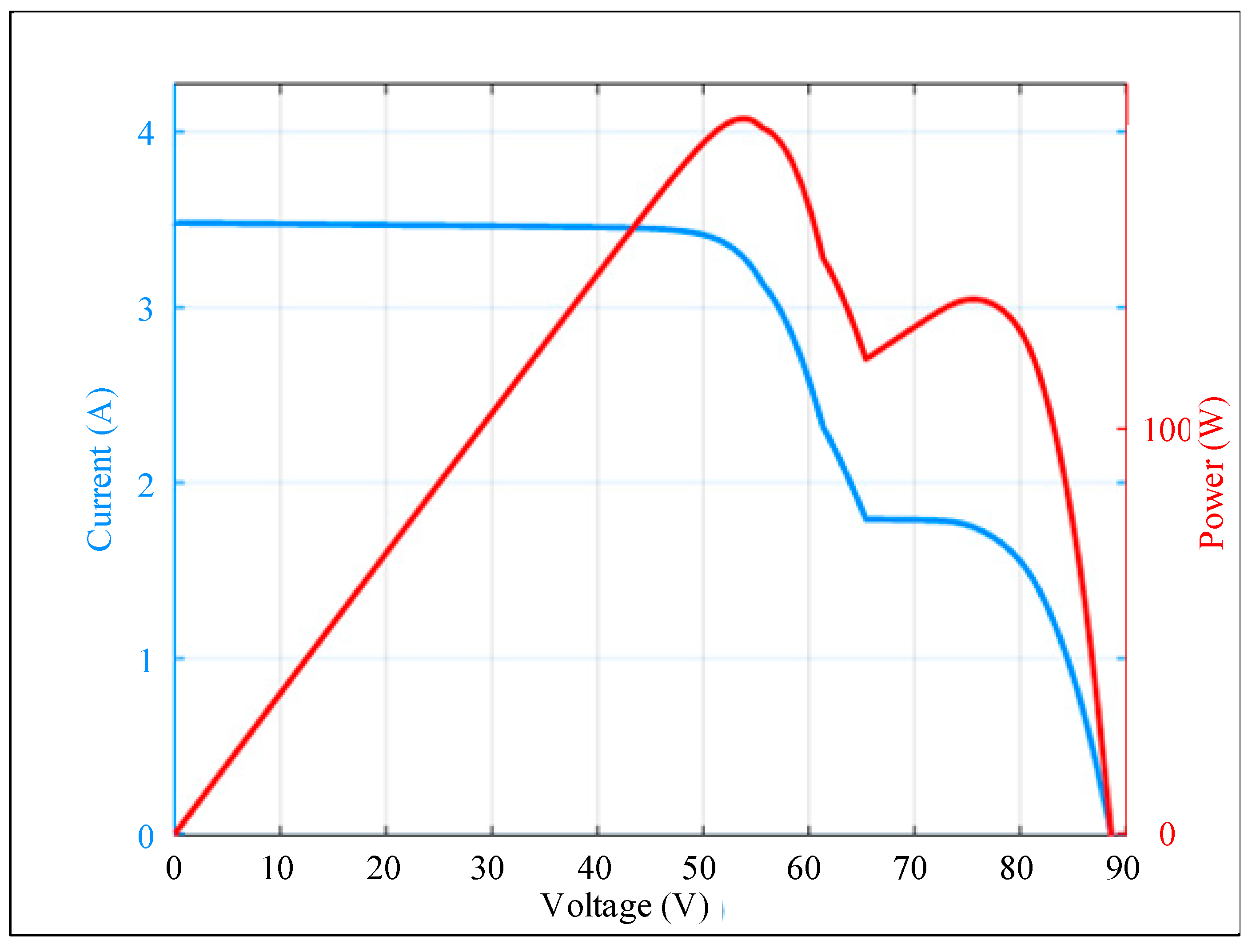
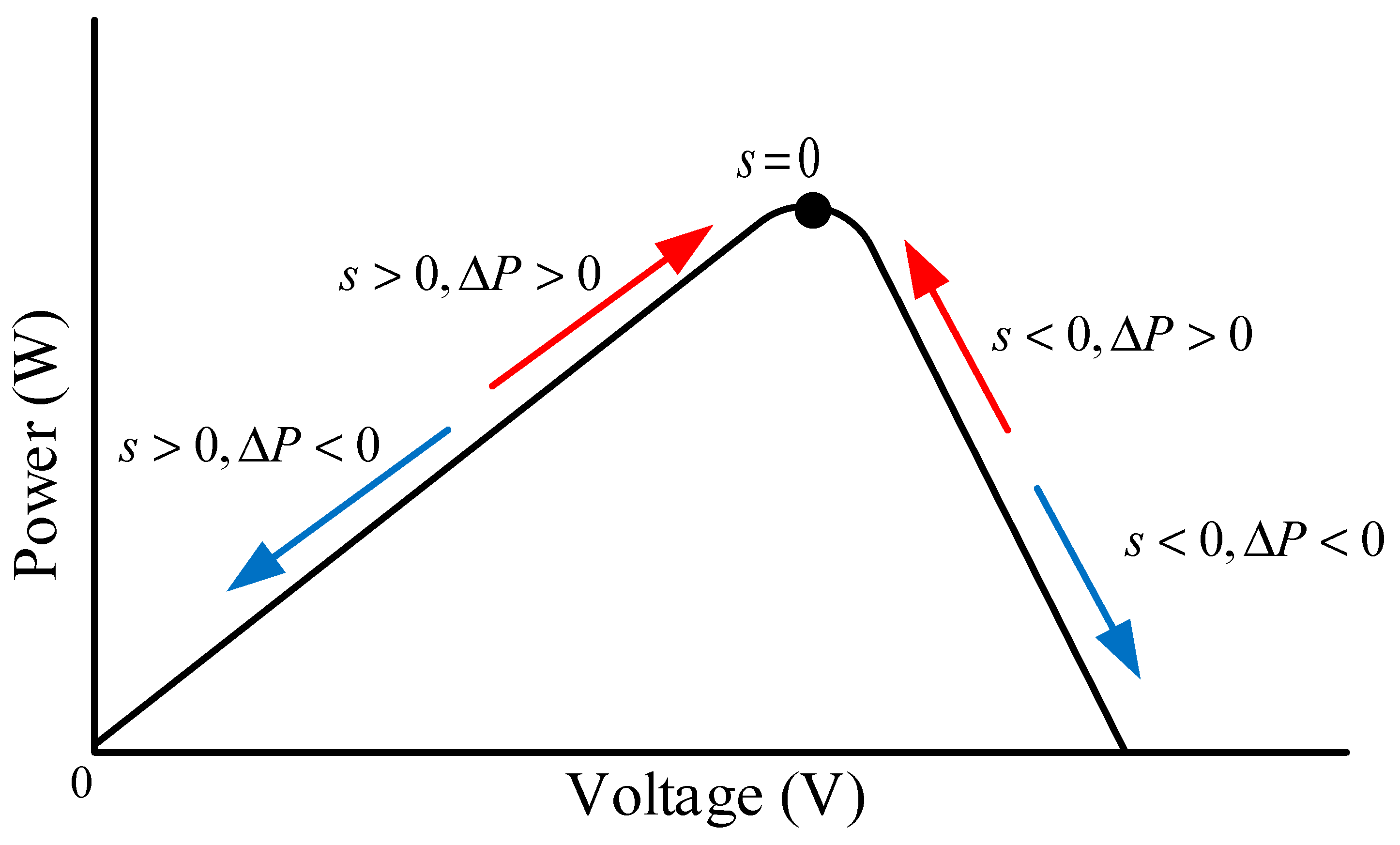
2. Properties of PMAs
3. GWOA
3.1. Conventional GWOA
- Step 1:
- The number of wolves and the maximum iteration number are configured, and the optimization parameters B, K, and α and the fitness value of each wolf are initialized.
- Step 2:
- The locations of the top three wolves with the largest fitness values are set as , , and , with , which denotes the location of the top wolf, being the current optimal solution.
- Step 3:
- Equation (1) is used to calculate the random distance between the location of each remaining wolf n and the locations of the top three wolves (i.e., , , and ), and Equations (2) and (3) are then used to update the location (i.e., fitness value) of each wolf n:
- Step 4:
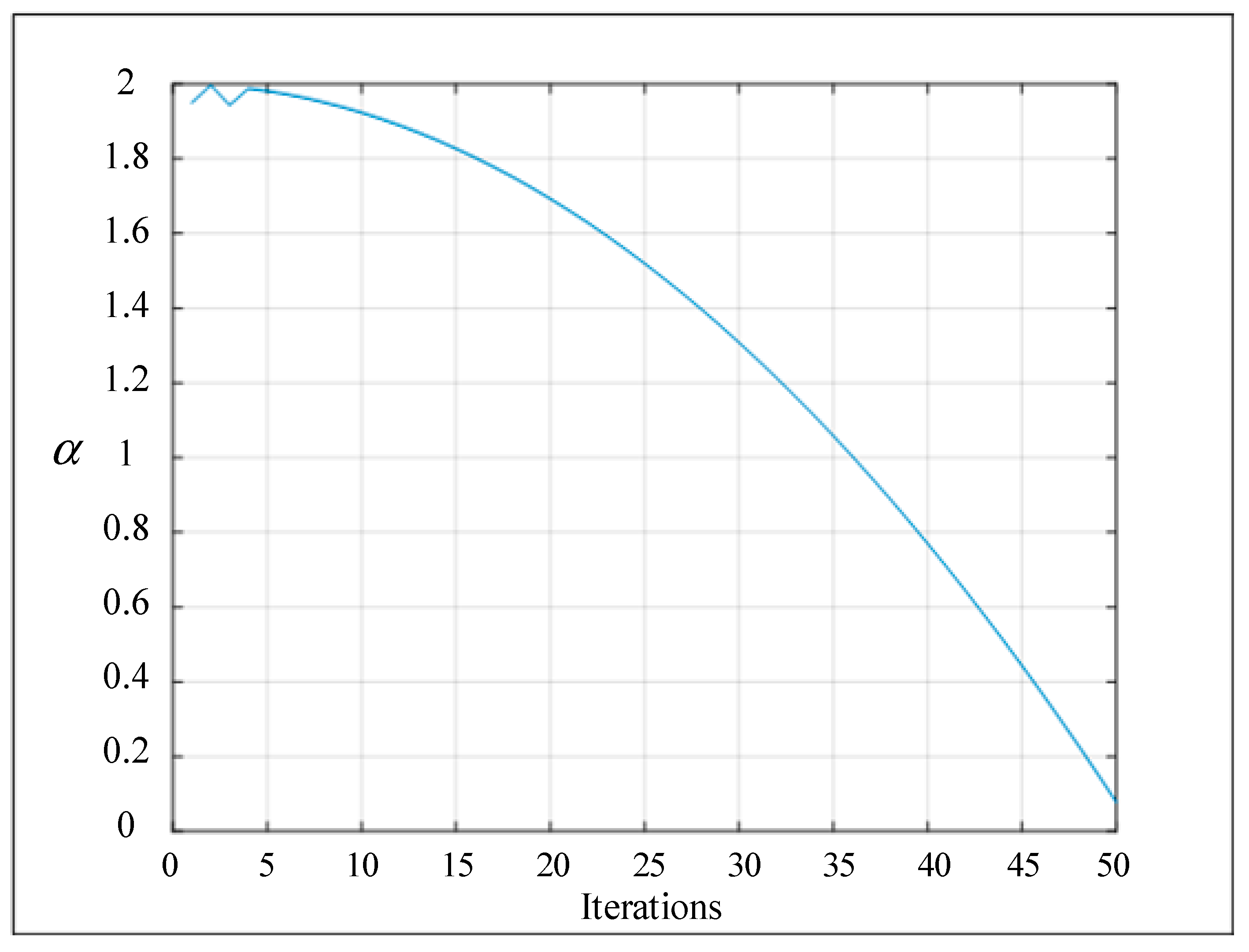
- Equations (4) and (5) are used to update the parameters B, K, and α:
- Step 5:
- When the iteration number reaches the preset maximum iteration number, the iteration process is terminated to record the top three fitness values (, , and ), and the optimal fitness value is output. If the preset conditions are not met, then the calculation process is repeated from Step 2.
3.2. Modified GWOA
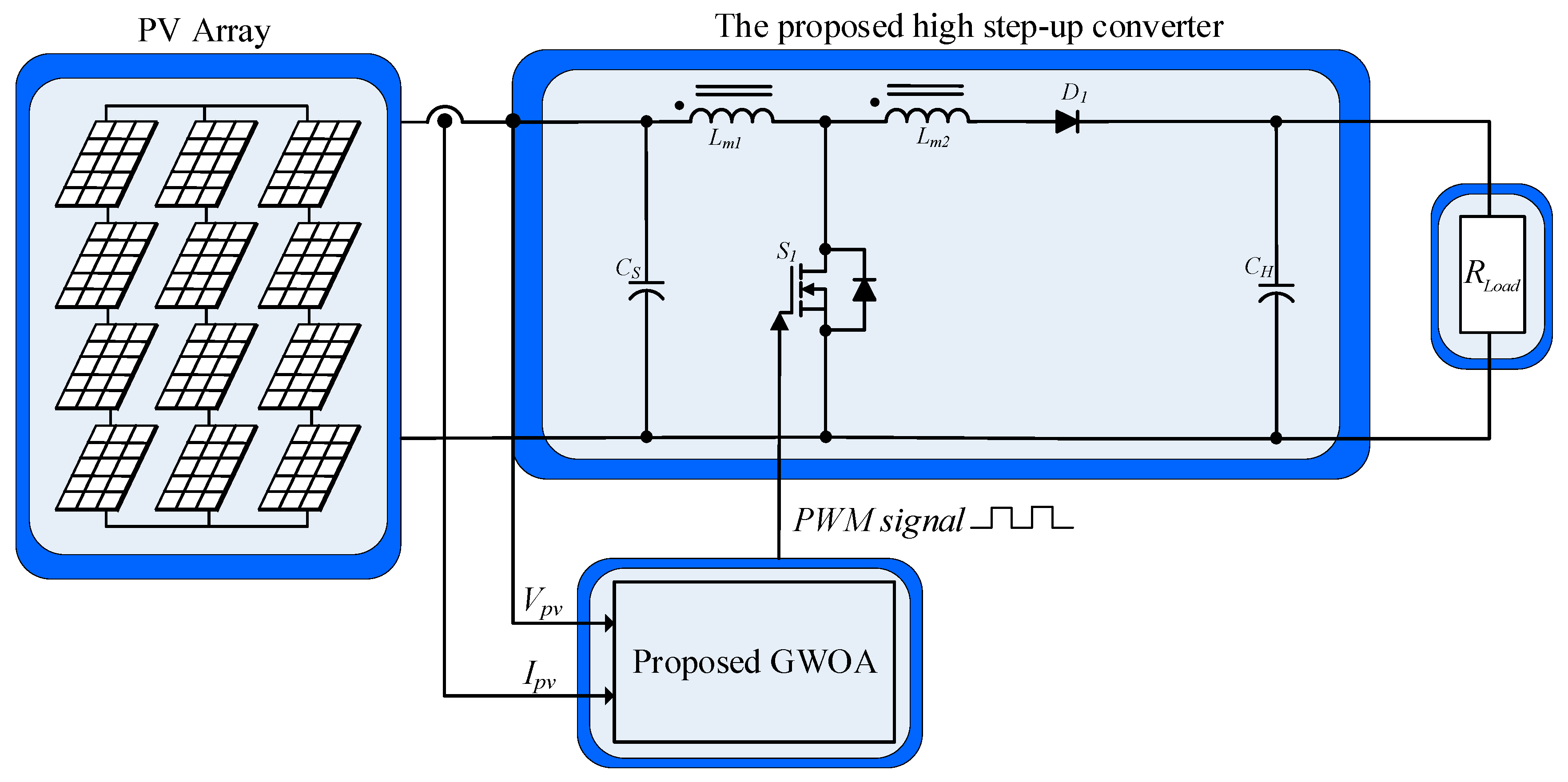
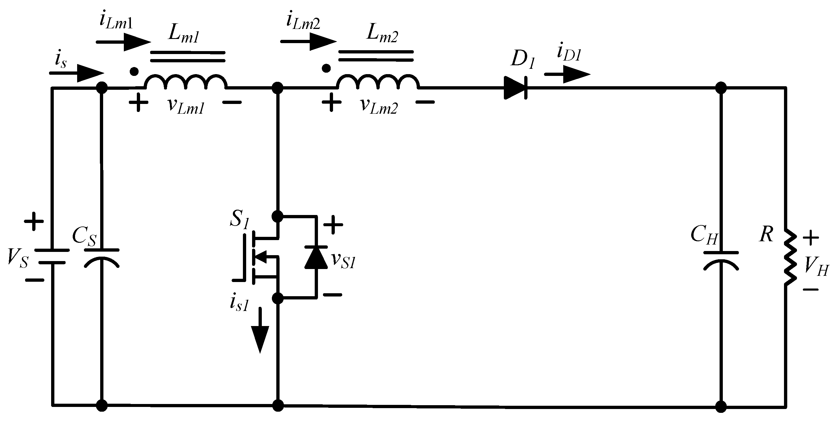
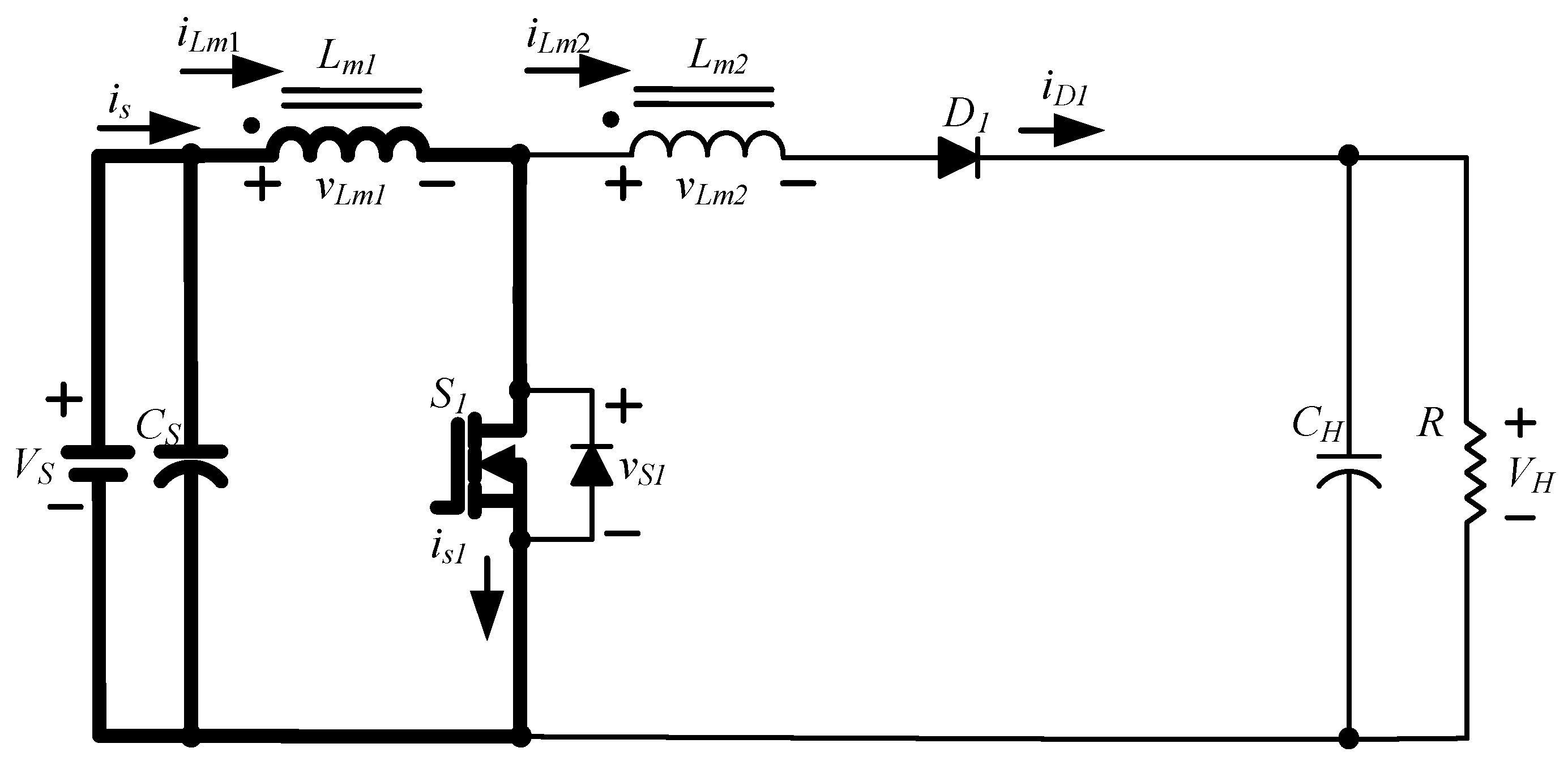
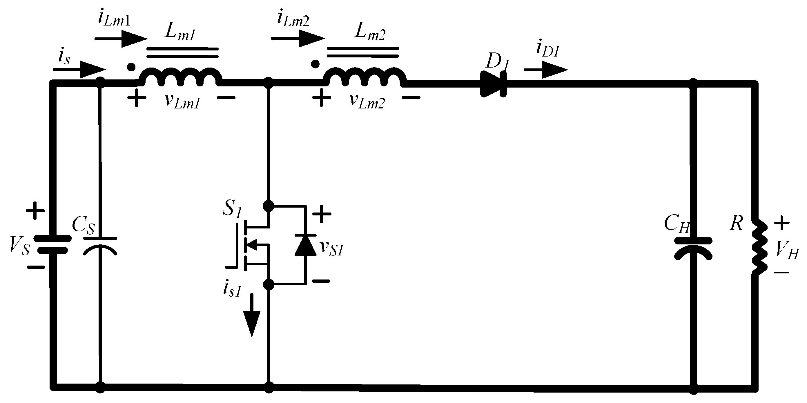
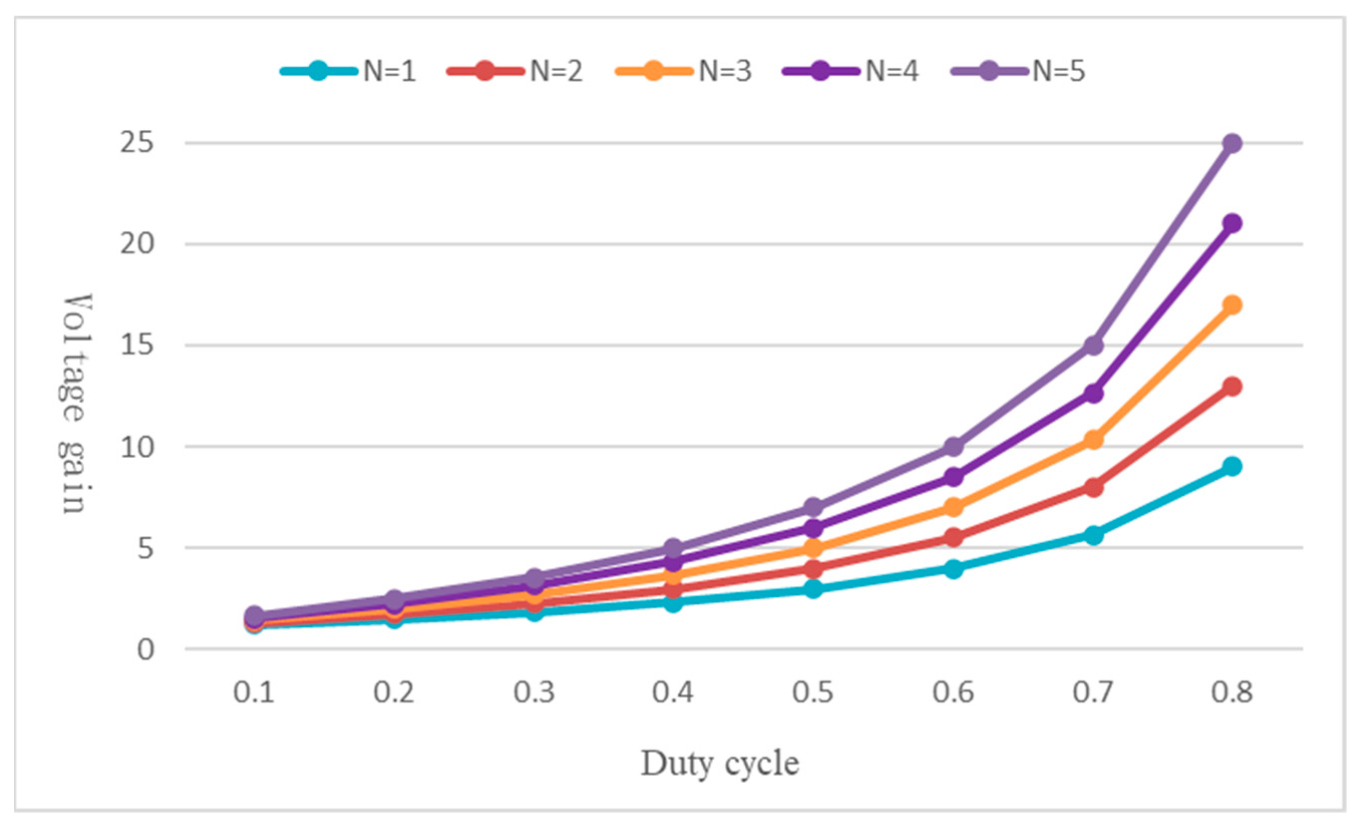
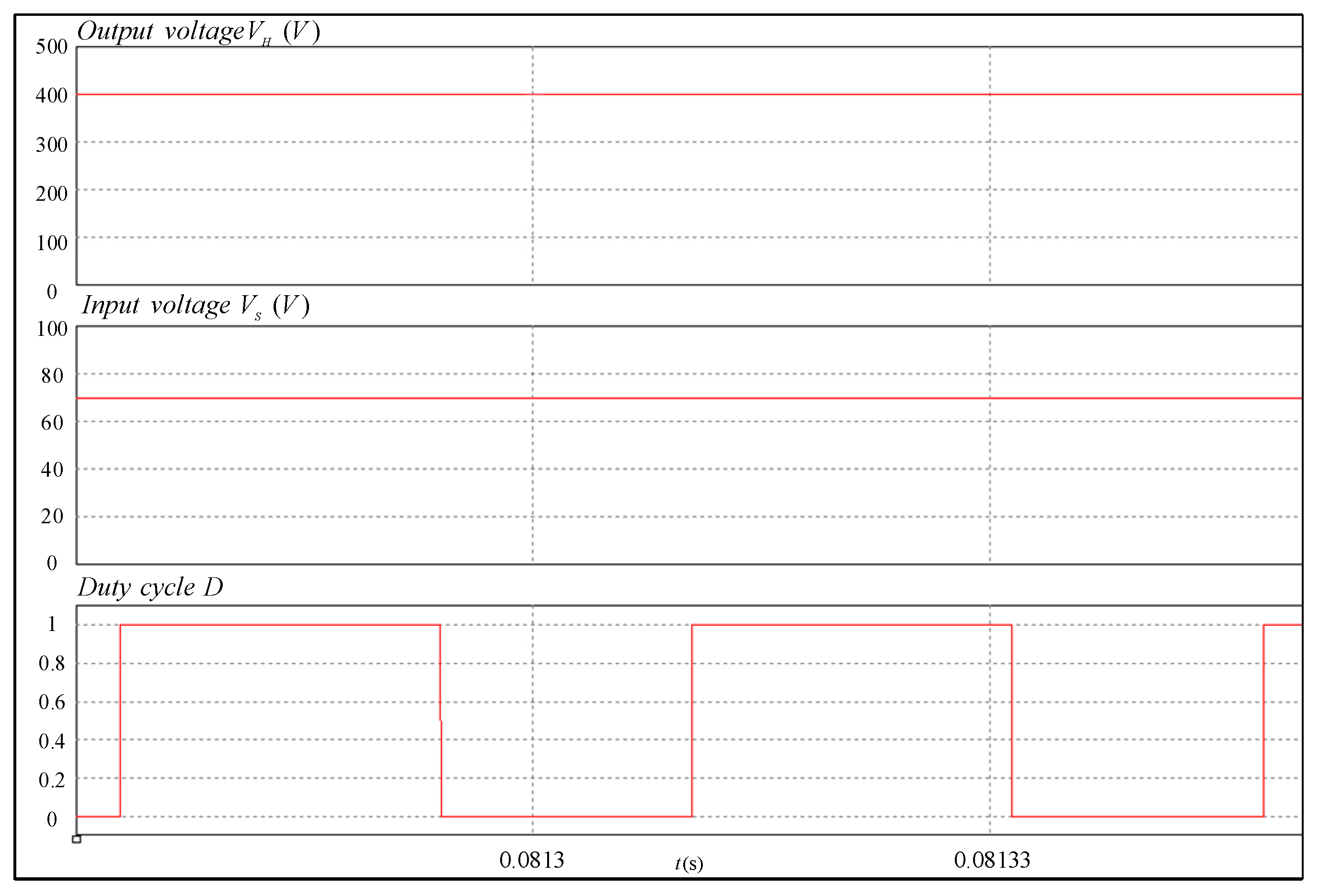
4. High-Voltage Step-Up Converter
4.1. Circuit Analysis of the High-Voltage Step-Up Converter
- (1)
- Switch on ()
- (2)
- Switch off ()
4.2. Design of Converter Elements
4.3. Design of the Main Inductor Element
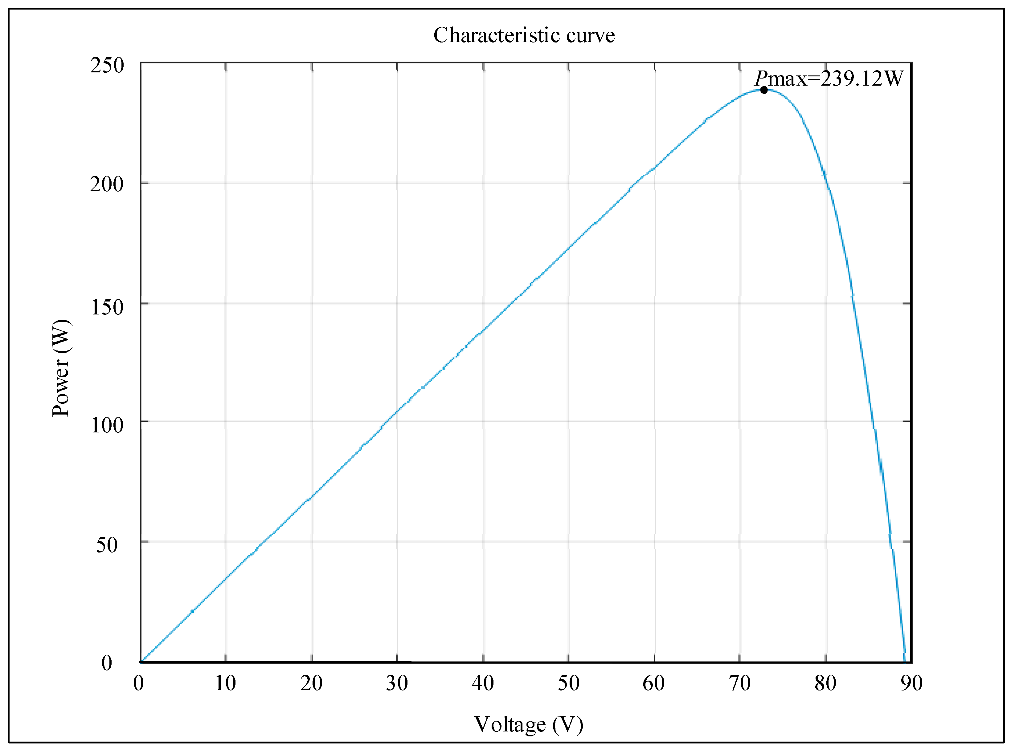
5. Simulation Results
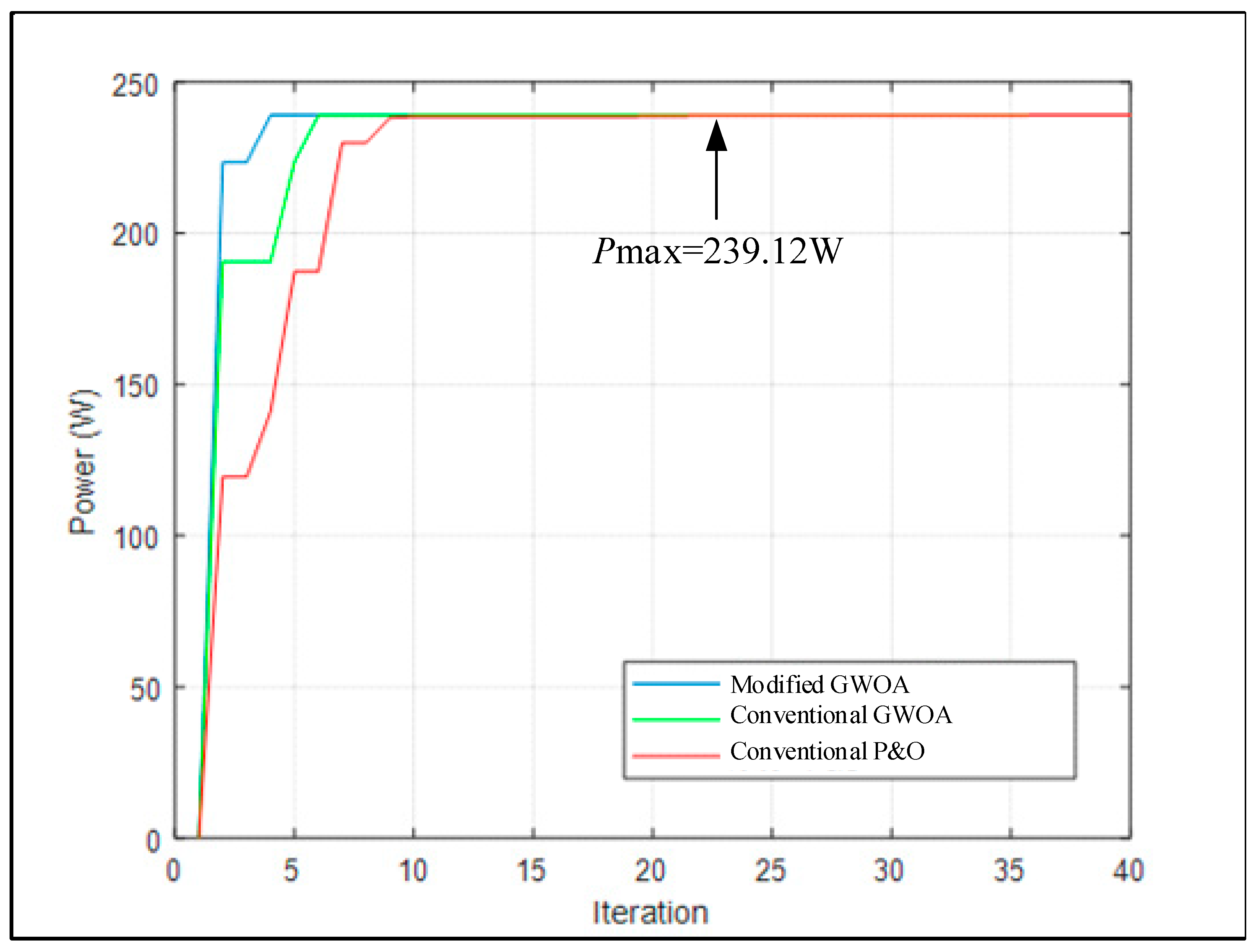
5.1. Simulation of the Modified GWOA
5.1.1. Case 1
5.1.2. Case 2
5.1.3. Case 3
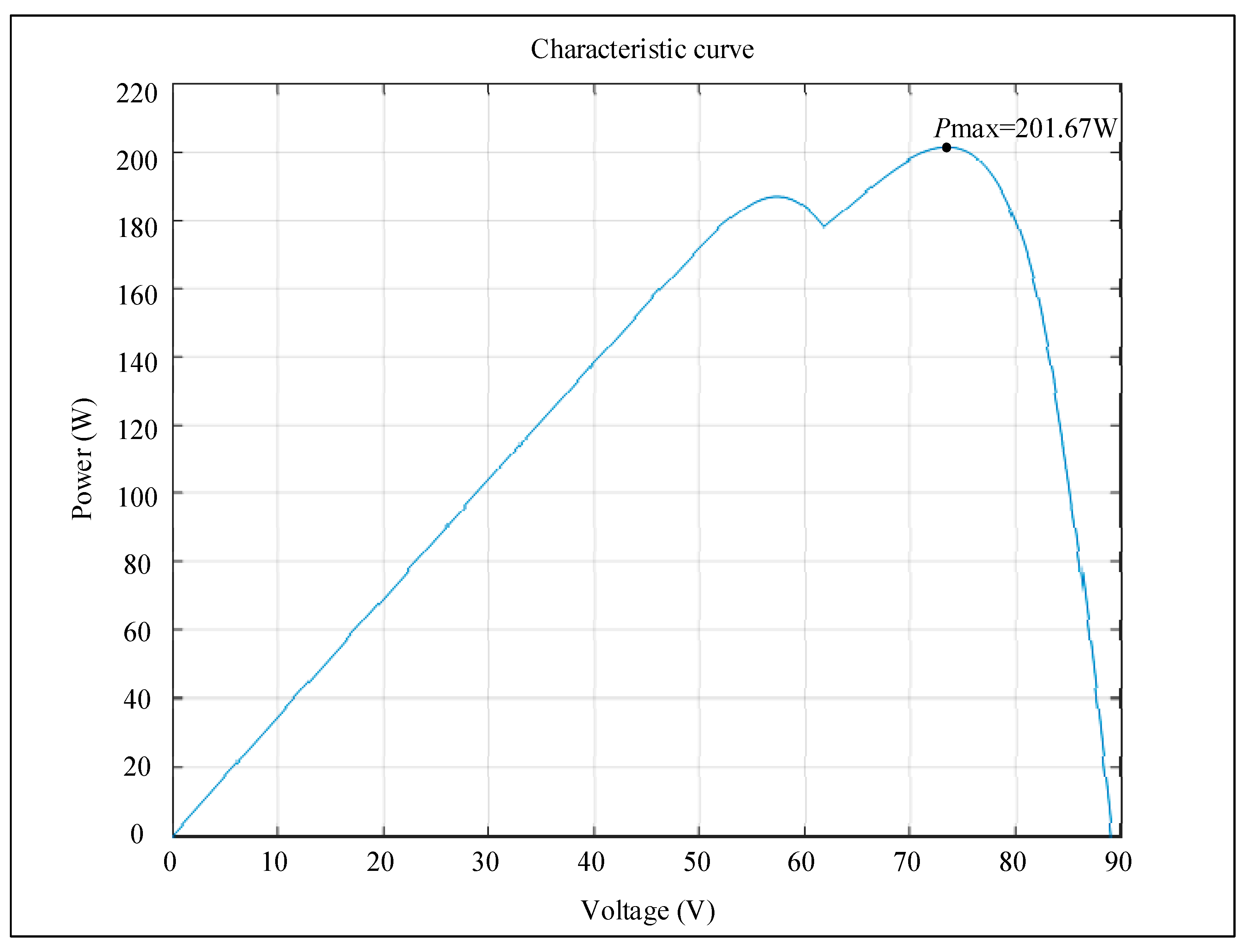
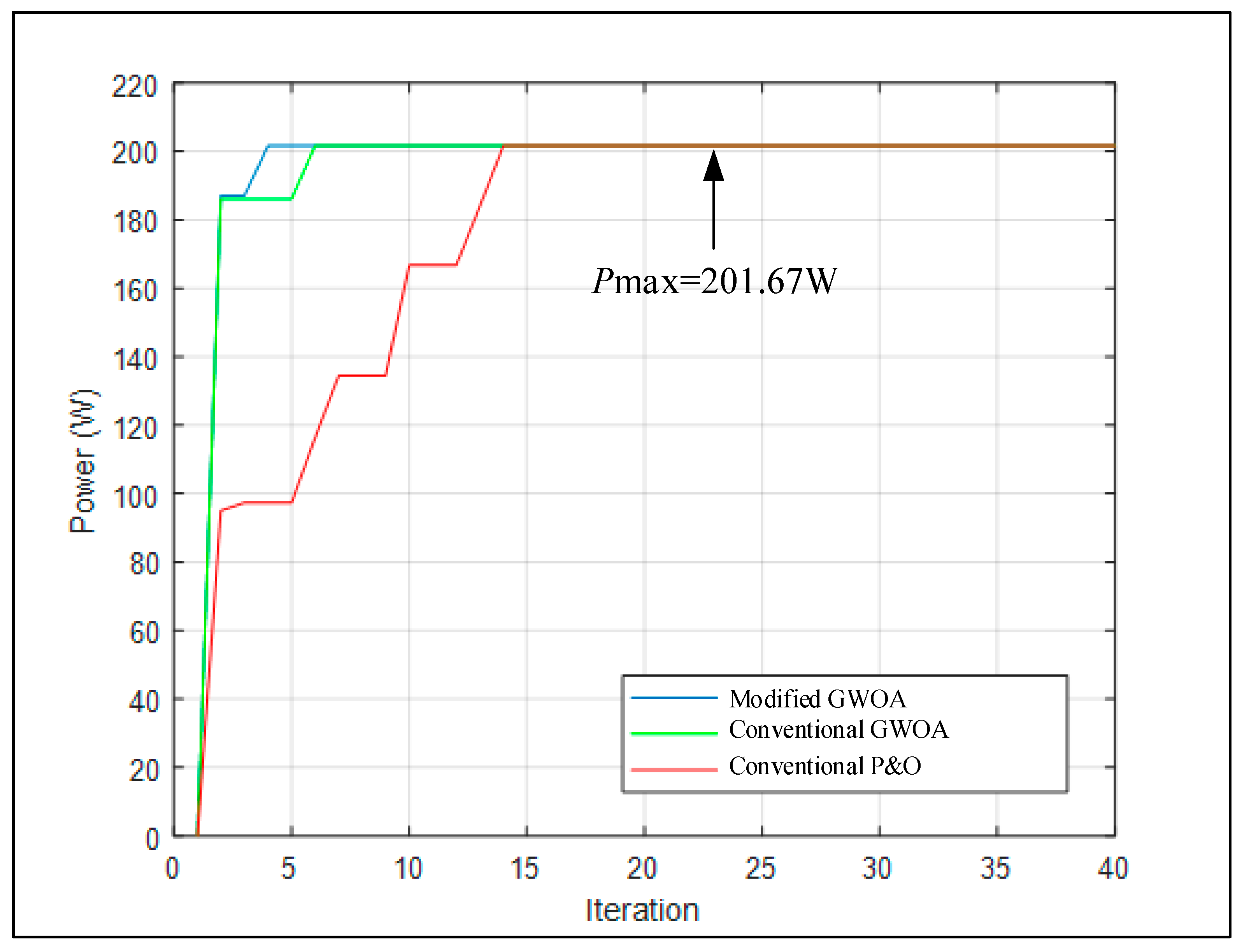
5.1.4. Case 4
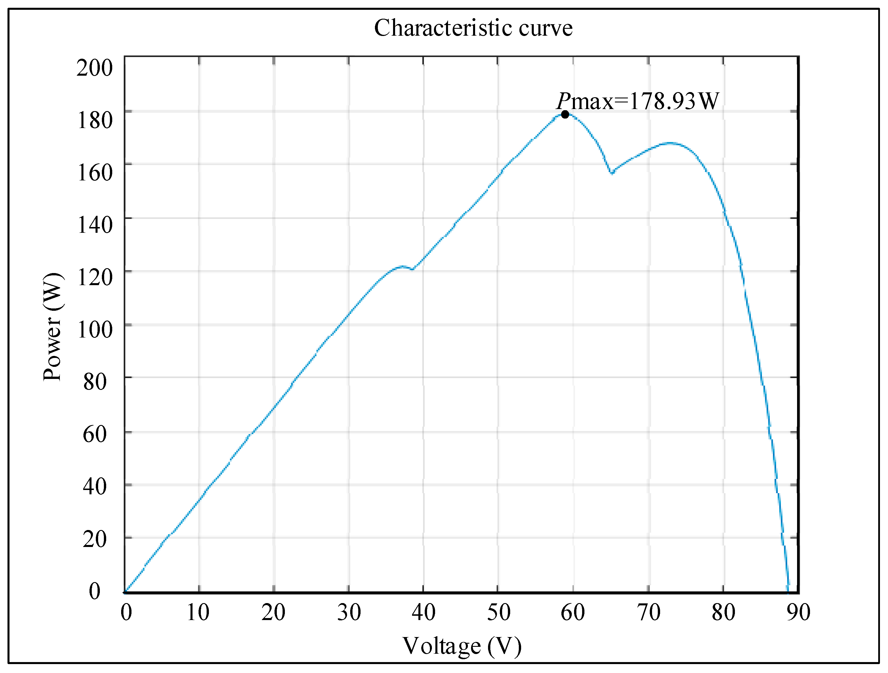
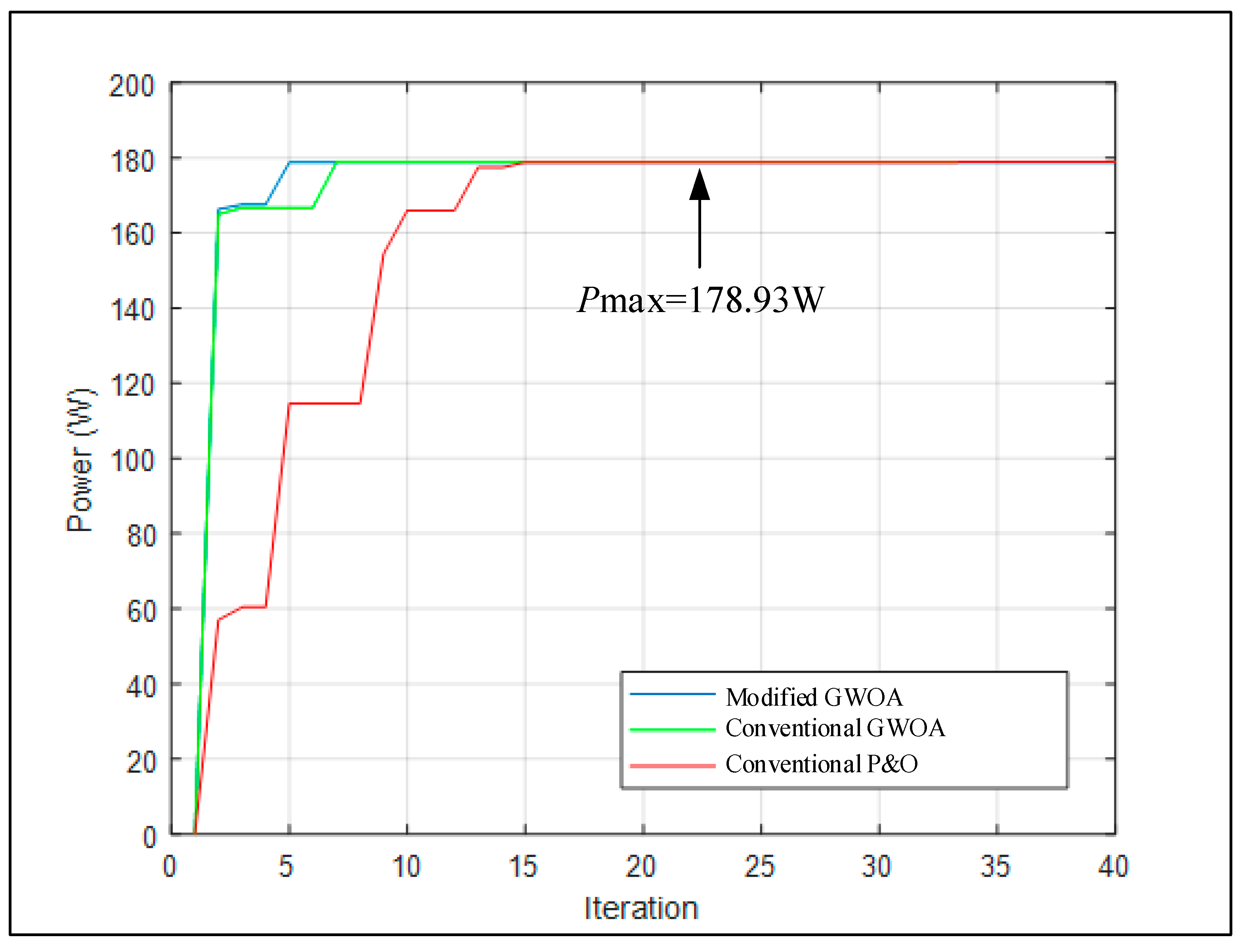
5.1.5. Case 5
5.2. Comparison of Different Tracking Algorithms in Each Case
6. Conclusions
Author Contributions
Funding
Data Availability Statement
Conflicts of Interest
References
- Sera, D.; Mathe, L.; Kerekes, T.; Spataru, S.V.; Teodorescu, R. On the Perturb-and-Observe and Incremental Conductance MPPT Methods for PV Systems. IEEE J. Photovolt. 2013, 3, 1070–1078. [Google Scholar] [CrossRef]
- Ahmed, J.; Salam, Z. An Enhanced Adaptive P&O MPPT for Fast and Efficient Tracking under Varying Environmental Conditions. IEEE Trans. Sustain. Energy 2018, 9, 1487–1496. [Google Scholar]
- Wang, J.; Yi, Y.; Yang, Y.; Zhang, G.; Huang, S. Research on Distributed Multi-peak Maximum Power Tracking Control. In Proceedings of the 29th Chinese Control and Decision Conference, Chongqing, China, 28–30 May 2017; pp. 2237–2341. [Google Scholar]
- Ma, Y.; Zhou, X.; Gao, Z.; Bai, T. Summary of the Novel MPPT (Maximum Power Point Tracking) Algorithm Based on Few Intelligent Algorithms Specialized on Tracking the GMPP (Global Maximum Power Point) for Photovoltaic Systems under Partially Shaded Conditions. In Proceedings of the 2017 IEEE International Conference on Mechatronics and Automation (ICMA), Takamatsu, Japan, 6–9 August 2017; pp. 311–315. [Google Scholar]
- Dorigo, M.; Birattari, M.; Stutzle, T. Ant Colony Optimization. IEEE Comput. Intell. Mag. 2006, 1, 28–39. [Google Scholar] [CrossRef]
- Dhieb, Y.; Yaich, M.; Bouzguenda, M.; Ghariani, M. MPPT Optimization Using Ant Colony Algorithm: Solar PV Applications. In Proceedings of the IEEE 21st international Ccnference on Sciences and Techniques of Automatic Control and Computer Engineering (STA), Sousse, Tunisia, 19–21 December 2022; pp. 503–507. [Google Scholar]
- Abdul, G.A.; Junita, M.S. Enhanced Global-Best Artificial Bee Colony Optimization Algorithm. In Proceedings of the Sixth UKSim/AMSS European Symposium on Computer Modeling and Simulation, Malta, Malta, 14–16 November 2012; pp. 95–100. [Google Scholar]
- González, C.; Restrepo, C.; Kouro, S.; Rodriguez, J. MPPT Algorithm Based on Artificial Bee Colony for PV System. IEEE Access 2021, 9, 43121–43133. [Google Scholar] [CrossRef]
- Pragallapati, N.; Sen, T.; Agarwal, V. Adaptive Velocity PSO for Global Maximum Power Control of a PV Array under Nonuniform Irradiation Conditions. IEEE J. Photovolt. 2017, 7, 624–639. [Google Scholar] [CrossRef]
- Li, H.; Yang, D.; Su, W.; Lü, J.; Yu, X. An Overall Distribution Particle Swarm Optimization MPPT Algorithm for Photovoltaic System under Partial Shading. IEEE Trans. Ind. Electron. 2019, 66, 265–275. [Google Scholar] [CrossRef]
- Megantoro, P.; Nugroho, Y.D.; Anggara, F.; Suhono; Rusadi, E.Y. Simulation and Characterization of Genetic Algorithm Implemented on MPPT for PV System under Partial Shading Condition. In Proceedings of the 2018 3rd International Conference on Information Technology, Information System and Electrical Engineering (ICITISEE), Yogyakarta, Indonesia, 13–14 November 2018; pp. 74–78. [Google Scholar]
- Rao, R.V.; Savsani, V.J.; Vakharia, D.P. Teaching-learning-Based Optimization: A Novel Method for Constrained Mechanical Design Optimization Problems. Comput. Aided Des. 2011, 43, 303–315. [Google Scholar] [CrossRef]
- Ahmed, J.; Salam, Z. A Soft Computing MPPT for PV System Based on Cuckoo Search Algorithm. In Proceedings of the 4th International Conference on Power Engineering, Energy and Electrical Drives, Istanbul, Turkey, 13–17 May 2013; pp. 558–562. [Google Scholar]
- Soneji, H.; Sanghvi, R.C. Towards the Improvement of Cuckoo Search Algorithm. In Proceedings of the 2012 World Congress on Information and Communication Technologies, Trivandrum, India, 30 October–2 November 2012; pp. 878–883. [Google Scholar]
- Nugraha, D.A.; Lian, K.L.; Suwarno. A Novel MPPT Method Based on Cuckoo Search Algorithm and Golden Section Search Algorithm for Partially Shaded PV System. J. Elect. Comput. Eng. 2019, 42, 173–182. [Google Scholar] [CrossRef]
- Lian, K.L.; Jhang, J.H.; Tian, I.S. A Maximum Power Point Tracking Method Based on Perturb-and-Observe Combined with Particle Swarm Optimization. IEEE J. Photovolt. 2014, 4, 626–633. [Google Scholar] [CrossRef]
- Daraban, S.; Petreus, D.; Morel, C. A Novel Global MPPT Based on Genetic Algorithms for Photovoltaic Systems under the Influence of Partial Shading. In Proceedings of the 39th Annual Conference of the IEEE Industrial Electronics Society, Vienna, Austria, 10–13 November 2013; pp. 1490–1495. [Google Scholar]
- Zhang, Y.M.; ASCE, S.M.; Wang, H.; ASCE, M.; Mao, J.X.; Xu, Z.D.; Zhang, Y.F. Probabilistic Framework with Bayesian Optimization for Predicting Typhoon-induced Dynamic Responses of a Long-Span Bridge. J. Struct. Eng. 2021, 147, 04020297. [Google Scholar] [CrossRef]
- Bollipo, R.B.; Mikkili, S.; Bonthagorla, K. Hybrid, Optimal, Intelligent and Classical PV MPPT Techniques: A Review. CSEE J. Power Energy Syst. 2021, 7, 9–33. [Google Scholar]
- Atici, K.; Sefa, I.; Altin, N. Grey Wolf Optimization Based MPPT Algorithm for Solar PV System with SEPIC Converter. In Proceedings of the 4th International Conference on Power Electronics and their Applications (ICPEA), Elazig, Turkey, 25–27 September 2019; pp. 1–6. [Google Scholar]
- Mohanty, S.; Subudhi, B.; Ray, P.K. A Grey Wolf Optimization Based MPPT for PV System under Changing Insolation Level. In Proceedings of the 2016 IEEE Students’ Technology Symposium (TechSym), Kharagpur, India, 30 September–2 October 2016; pp. 175–179. [Google Scholar]
- Subudhi, B.; Pradhan, R. A Comparative Study on Maximum Power Point Tracking Techniques for Photovoltaic Power Systems. IEEE Trans. Sustain. Energy 2013, 4, 89–98. [Google Scholar] [CrossRef]
- Millah, I.S.; Chang, P.C.; Teshome, D.F.; Subroto, R.K.; Lian, K.L.; Lin, J. An Enhanced Grey Wolf Optimization Algorithm for Photovoltaic Maximum Power Point Tracking Control under Partial Shading Conditions. IEEE J. Ind. Electron. Soc. 2022, 3, 392–408. [Google Scholar] [CrossRef]
- SunWorld Datasheet. Available online: http://www.ecosolarpanel.com/ecosovhu/products/18569387_0_0_1.html (accessed on 12 January 2023).
- Narasimharaju, B.L.; Dubey, S.P.; Singh, S.P. Coupled Inductor Bidirectional DC-DC Converter for Improved Performance. In Proceedings of the 2010 International Conference on Industrial Electronics, Control and Robotics, Rourkela, India, 27–29 December 2010; pp. 27–29. [Google Scholar]


| Parameter | Value |
|---|---|
| Maximum output power (Pmax) | 20 W |
| MPP current (IMPP) | 1.10 A |
| MPP voltage (VMPP) | 18.18 V |
| Short-circuit current (ISC) | 1.15 A |
| Open-circuit voltage (VOC) | 22.32 V |
| Criterion | |||
| No | |||
| 1 | |||
| 2 | |||
| 3 | |||
| 4 | |||
| 5 | |||
| 6 | |||
| 7 | |||
| 8 | |||
| 9 | |||
| 10 | |||
| 11 | |||
| Parameter | Value |
|---|---|
| Low-voltage side direct input voltage (VS) | VS = 70 V ± 10% |
| High-voltage side direct output voltage (VH) | VH = 400 V |
| Switching frequency (f) | f = 25 kHz |
| Coupled inductor turns ratio (N) | |
| Rated output power (P) | P = 300 W |
| Case | Module Connection and Shading Condition | Number of P–V Curve Peaks |
|---|---|---|
| 1 | Three parallel strings, with each string comprising four modules connected in series: (0% shading + 0% shading + 0% shading + 0% shading)// (0% shading + 0% shading + 0% shading + 0% shading)// (0% shading + 0% shading + 0% shading + 0% shading) | One |
| 2 | Three parallel strings, with each string comprising four modules connected in series: (0% shading + 0% shading + 0% shading + 50% shading)// (0% shading + 0% shading + 0% shading + 0% shading)// (0% shading + 0% shading + 0% shading + 0% shading) | Two (MPP was on the right peak) |
| 3 | Three parallel strings, with each string comprising four modules connected in series: (0% shading + 0% shading + 30% shading + 90% shading)// (0% shading + 0% shading + 0% shading + 0% shading)// (0% shading + 0% shading + 0% shading + 0% shading) | Three (MPP was on the middle peak) |
| 4 | Three parallel strings, with each string comprising four modules connected in series: (0% shading + 30% shading + 50% shading + 70% shading)// (0% shading + 0% shading + 0% shading + 0% shading)// (0% shading + 0% shading + 0% shading + 0% shading) | Four (MPP was on the rightmost peak) |
| 5 | Three parallel strings, with each string comprising four modules connected in series: (0% shading + 10% shading + 80% shading + 90% shading)// (0% shading + 10% shading + 80% shading + 90% shading)// (0% shading + 10% shading + 80% shading + 90% shading) | Four (MPP was on the second peak from the left) |
| Case | Number of Peaks on the P–V Curve | Mean Iteration Number | ||
|---|---|---|---|---|
| Conventional P&O Algorithm | Conventional GWOA | Modified GWOA | ||
| 1 | One | 11.4 | 8.6 | 7.5 |
| 2 | Two (MPP on the right peak) | 17.2 | 12.5 | 9.6 |
| 3 | Three (MPP on the middle peak) | 21.2 | 13.5 | 11.6 |
| 4 | Four (MPP on the rightmost peak) | Failed | 20.8 | 15.2 |
| 5 | Four (MPP on the second peak from the left) | 25.6 | 17.5 | 15.6 |
| Case | Number of Peaks on the P–V Curve | Tracking Efficiency (%) | ||
|---|---|---|---|---|
| Conventional P&O Algorithm | Conventional GWOA | Modified GWOA | ||
| 1 | One | 76.46% | 91.69% | 98.15% |
| 2 | Two (MPP on the right peak) | 68.84% | 97.26% | 98.48% |
| 3 | Three (MPP on the middle peak) | 72.34% | 97.41% | 98.41% |
| 4 | Four (MPP on the rightmost peak) | 36.73% | 90.74% | 94.85% |
| 5 | Four (MPP on the second peak from the left) | 58.53% | 88.43% | 94.62% |
Disclaimer/Publisher’s Note: The statements, opinions and data contained in all publications are solely those of the individual author(s) and contributor(s) and not of MDPI and/or the editor(s). MDPI and/or the editor(s) disclaim responsibility for any injury to people or property resulting from any ideas, methods, instructions or products referred to in the content. |
© 2023 by the authors. Licensee MDPI, Basel, Switzerland. This article is an open access article distributed under the terms and conditions of the Creative Commons Attribution (CC BY) license (https://creativecommons.org/licenses/by/4.0/).
Share and Cite
Huang, K.-H.; Chao, K.-H.; Kuo, Y.-P.; Chen, H.-H. Maximum Power Point Tracking of Photovoltaic Module Arrays Based on a Modified Gray Wolf Optimization Algorithm. Energies 2023, 16, 4329. https://doi.org/10.3390/en16114329
Huang K-H, Chao K-H, Kuo Y-P, Chen H-H. Maximum Power Point Tracking of Photovoltaic Module Arrays Based on a Modified Gray Wolf Optimization Algorithm. Energies. 2023; 16(11):4329. https://doi.org/10.3390/en16114329
Chicago/Turabian StyleHuang, Kuo-Hua, Kuei-Hsiang Chao, Ying-Piao Kuo, and Hong-Han Chen. 2023. "Maximum Power Point Tracking of Photovoltaic Module Arrays Based on a Modified Gray Wolf Optimization Algorithm" Energies 16, no. 11: 4329. https://doi.org/10.3390/en16114329
APA StyleHuang, K.-H., Chao, K.-H., Kuo, Y.-P., & Chen, H.-H. (2023). Maximum Power Point Tracking of Photovoltaic Module Arrays Based on a Modified Gray Wolf Optimization Algorithm. Energies, 16(11), 4329. https://doi.org/10.3390/en16114329