Abstract
It is well known that thermal conductivity measurement is a challenging task, due to the weaknesses of the traditional methods, such as the high cost, complex data analysis, and limitations of sample size. Nowadays, the requirement of quality of life and tightening energy efficiency regulations of buildings promote the demand for new construction materials. However, limited by the size and inhomogeneous structure, the thermal conductivity measurement of wall samples becomes a demanding topic. Additionally, we find the thermal parameter values of the samples measured in the laboratory are different from those obtained by theoretical computation. In this paper, a novel signal-transmissive wall is designed to provide the problem solving of signal connectivity in 5G. We further propose a new thermal conductivity predictor based on the Harmony Search (HS) algorithm to estimate the thermal properties of laboratory-made wall samples. The advantages of our approach over the conventional methods are simplicity and robustness, which can be generalized to a wide range of solid samples in the laboratory measurement.
1. Introduction
With the development of modern technology, as well as the demands of zero-energy buildings, the thermal performance assessment of new building walls has gained more and more research attention during the past decade. The contradiction between the improvement of quality of life and addressing the ongoing energy crisis has led to the emergence of new construction materials. For example, the fifth generation of mobile technology (5G) has created smart and networked communication environments that connect people, devices, data, applications, transport systems, and cities [1,2,3,4]. As a result of the high operational radio frequencies and increasingly stringent energy efficiency regulations for buildings, more than 70% of cell phone users in the buildings are dissatisfied with the current fourth- and fifth-generation cellular technologies. New types of energy-efficient buildings indeed incorporate structures, such as low-emissive windows and multi-layered thermal insulation, which are highly effective in blocking radio signals. A novel type of signal-transmissive wall with the embedded passive antennas has been developed to address the challenge of wireless connectivity in both the current low-energy and future zero-energy buildings [5].
The distributed antennas are embedded on both wall sides connected via appropriate microwave circuits. In other words, this signal-transmissive wall allows radio signal to penetrate into the low-energy buildings in the urban setting. However, the impact on the thermal performance becomes a significant challenge and plays a crucial role in determining the feasibility of this new antennas-embedded wall [6,7,8,9]. Furthermore, we have found that the thermal parameter values obtained through laboratory measurement differed from those obtained through theoretical computation. There are some certain limitations of the traditional thermal conductivity measurement approaches, for example, the intricate heat insulation and long measurement time of steady-state methods and the high costs induced by the instruments of transient methods [10,11,12,13,14,15]. Additionally, unlike the small-size laboratory samples, it is difficult to utilize the traditional instruments for measuring the parameters, such as conductivity and specific heat of the signal-transmissive wall due to the thick inhomogeneous structure. Therefore, an effective method to find whether the wall retains high thermal insulation is desired. Based on the artificial intelligence (AI) optimization algorithm, this paper proposes a novel thermal conductivity assessment technique with the advantages of low cost, robustness, and simplicity.
To analyze the thermal performance of the signal-transmissive wall, the laboratory test was carried out on two identical multi-layered structure samples, the reference (conventional wall) and the antenna-embedded model. In our AI predictor, the Harmony Search (HS) algorithm, a population-based random search method, was employed to find the optimal value of thermal conductivity. It had the ability to work without any prior domain knowledge and constraints imposed on the given problem, such as gradient information of the objective functions.
In contrast to other population-based optimization techniques, it employed only one candidate pool, Harmony search Memory (HM), to evolve [16,17]. Due to few mathematical requirements, the HS had a significant advantage in terms of computational simplicity that could bring the benefit of reducing the corresponding computational burden in heat transfer calculation. Moreover, its stochastic nature resulted in the flexibility, randomness, and robustness, which were suitable for the inhomogeneous model analysis.
In this paper, we first introduce the two laboratory models (the sandwich reference wall and the signal-transmissive wall samples) in Section 2. The traditional thermal conductivity measurement methods are reviewed in Section 3. In Section 4, the proposed thermal conductivity predictor is presented and explained. The experimental results and analysis are provided in the following section. Section 6 summarizes and concludes our paper with remarks and improvements.
2. Laboratory Samples
Two bare load-bearing wall samples with sandwich structures were compared to study the thermal performance of the proposed signal-transmissive wall. The one without a 5G antenna was considered as the reference sample, and its general structure is shown in Figure 1. The wall with a section of 15.00 cm × 15.00 cm consisted of a layer of rock wool insulation that was 20.50 cm thick. The two layers of sandwiched concrete were 7.50 cm and 15.00 cm thick, respectively.
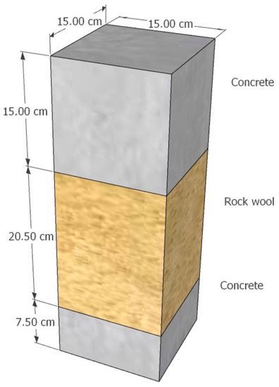
Figure 1.
General structure of reference sample.
Another sample was the signal-transmissive wall sample, which included an integrated ultrawideband back-to-back spiral antenna system within the sandwiched structure [18]. As illustrated in Figure 2, the antenna system consisted of two identical spiral antennas and a semi-rigid dual coaxial cable, which were installed at the center of the wall. In this sample, the spiral antenna was composed of a copper two-arm spiral, which was 0.035 mm thick and had an outer radius of 17.4 mm and an inner radius of 1.08 mm. The antenna was mounted on a Rogers RT/Duroid 5880 PCB that was 0.5 mm thick and a Styrofoam board that was 10 mm thick. The semi-rigid dual coaxial cable consisted of a rubber block and two coaxial cables. Each coaxial cable comprised a stainless steel outer connector, a PTFE (Teflon) dielectric block, and a stainless steel center connector. The two center connectors were connected to the spiral arms, while the remaining elements of the dual coaxial cable touched the PCBs. The PCB was embedded in the Styrofoam board to the same level as the concrete [19].
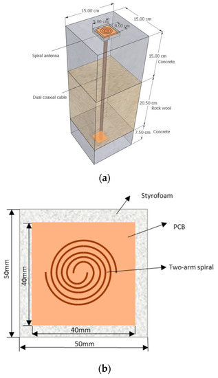
Figure 2.
(a) General structure of signal-transmissive wall sample. (b) Spiral antenna.
These two samples had the same general sizes and main materials. Table 1 gives the detailed parameters of both samples.

Table 1.
Properties of two samples.
3. Conventional Thermal Conductivity Measurement Approaches
Thermal conductivity refers to a material’s capacity to conduct heat and indicates the rate at which temperature differences transmit through a material [7]. Aided by increasingly advanced instruments, many methods have been employed for the thermal conductivity measurements of various materials, including homogeneous, inhomogeneous, and even liquid materials spanning a broad temperature range. This section presents two types of widely used traditional measurement schemes: steady- and transient-state methods.
3.1. Steady-State Methods
The thermal conductivity can be achieved based on steady-state measurements, which measure the temperature difference at a given distance while the heat flow passes through the sample. In the measurement, the steady-state condition is obtained when the temperature gradient across the sample is constant over time. The four widely employed methods are the comparative cut bar technique, the absolute technique, the radial heat flow method, and the parallel thermal conductance technique [13]. The steady-state methods have several advantages over the others because of their simplicity and versatility for a wide range of materials [14,15,20]. They typically require fewer experimental parameters and can be easily automated, making them more efficient and cost-effective. For example, the guarded hot plate method only requires the temperature difference between the hot and cold plates. However, the main drawback of the steady-state methods is the error caused by heat losses in the laboratory setup, which is due to the heat transfer of radiation and convection. Additionally, errors caused by sample thickness can affect the accuracy of the measurement results as well.
3.2. Transient State Methods
The transient state methods apply a heat pulse to the sample and measure the resulting transient temperature change on one or more locations in the sample. The measurements are usually carried out using temperature sensors, such as a thermocouple and a resistance thermometer. This non-destructive approach can be utilized to measure the thermal properties of a broad range of materials in solid, liquid, and gaseous states. The popular transient state approaches are the transient line source method, the pulsed power technique, the hot-wire method, the transient plane source method, and the laser flash method [21,22,23]. For example, the transient plane source method uses a special mathematical model, a continuous plane heat source, and a small sensor (plane source) sandwiched between the two halves of sample. The heat is transferred through the sample, causing a temporary change at the surface of the plane source. This change can be detected by a sensor located on the opposite side of the plane source. The transient schemes have certain advantages over the steady-state methods in terms of heat losses, contact resistance of temperature sensors, and measurement time. On the other hand, they have many drawbacks, including the sample geometry limitation, complexity and high cost of equipment. For instance, to obtain accurate results using the transient state method, a small size sample with a homogeneous structure is usually required because the heat flows uniformly through the material, and any variations in the sample’s composition and structure can affect the measurement results. In other words, the transient state methods are not suitable for thermal conductivity measurement of anisotropic or inhomogeneous samples, e.g., the reference and signal-transmissive wall samples used in this paper. Additionally, transient methods often require the use of expensive instruments.
4. Novel Thermal Conductivity Estimation Method
As previously mentioned, both the steady- and transient-state methods have their own inherent drawbacks that limit the practical thermal conductivity measurement in laboratories. To address this issue, we proposed a novel thermal conductivity measurement method called the AI-based conductivity predictor in this paper. Our technique was based on predicting the thermal conductivity of large samples with inhomogeneous material. By leveraging the harmony search method, a branch of artificial intelligence algorithms, it could provide simpler and more reliable measurements in large size sample thermal property estimation.
4.1. Laboratory Measurement Setup
The reference and antenna-embedded samples consisted of the same multi-layered structure, as given in Table 1. Compared with the reference model, there was an antenna installed in the signal-transmissive wall. To imitate the real-world conditions, the bottom concrete layer was treated as the exterior wall that was exposed to lower temperatures. In the laboratory measurement, the cooling thermostats (type: Lauda RE 1050 eco silver) were utilized to control the temperature at the bottom surfaces of the models. The other faces, including the top surface of the concrete, were left uncovered (without insulation), which meant that their temperature depended on the ambient temperature. The laboratory temperature was monitored by a data logger and kept at 22 °C, which was considered as both the initial model temperature and the boundary condition in the MATLAB simulations. This approach can help to control the heat flow and boundary condition, thereby minimizing the measurement errors.
The cooling bed connected with the thermostats was a square with a 40 cm inner length (larger than that of the samples), and its edge had 10 cm height. Because the cooling bed size was larger than that of the sample section, there was unintended heat transfer generated through radiation from the uncovered area of the cooling bed to the samples. This could lead to a change in the ambient temperature through convection. To achieve the ideal measurement environment and boundary conditions, the samples were first lifted to the height of the cooling bed sides by adding a high-conductivity steel base that had the same shape as the sample section. Next, the uncovered cooling plate area and steel base were insulated using rock wool and extruded polystyrene (XPS) as shown in Figure 3. Steel was the perfect type of material for the base due to its heat conduction performance and low cost. After adding the insulation layer, the top surface temperature of the base was almost that of the cooling bed. Additionally, it was confirmed that heat transfer from the insulated cooling bed could be neglected.
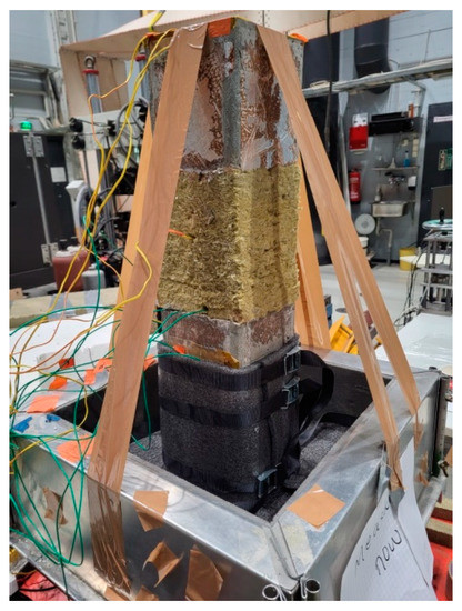
Figure 3.
Sample measurement.
The object of our work was to compare the thermal conductivities of these two samples to obtain the thermal properties of the signal-transmissive wall. Therefore, we compared their thermal performances by analyzing temperature profiles with the cooling temperature −5 °C at the sample bottoms. There were 12 sampling points located at the bottom, two layer intersections, and the top of the samples, as illustrated in Figure 4. Two data loggers, Hioki LR8431-20 (range of measurements: −200 °C to 2000 °C, max. resolution: 0.1 °C and accuracy: ±0.5 °C) and Pico TC-08 (range of measurements: −250 °C to 1370 °C, max. resolution: 0.025 °C and accuracy: ±0.5 °C), were employed to acquire the temperatures at these sampling points. Because we aimed at comparing the performance of heat transfer, the positions of the sampling points were the same in both the reference and the signal-transmissive wall models.
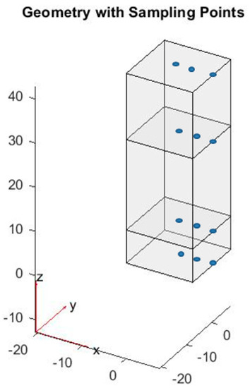
Figure 4.
Sampling locations of two models.
The thermal data indicated that the trigger time was 22 November 2022, at 4:11:03 P.M. The measurement results obtained at 0, 500, 1000, 1500, 2000, and 2500 min are presented in Figure 5, where the x axis and y axis represent the sample height and temperature, respectively. The temperatures of the sampling points were around 23 °C (room temperature) at the initial state (0 min). However, the lower sampling points experienced rapid temperature changes within 2500 min. For instance, the temperature at the sampling point located at a height of 12.5 cm (the intersection between the first concrete and rock wool layer) decreased from 23 °C at 0 min to 6.2 °C after 500 min and remained at 5.3 °C after 1000 min. The thermal performances of the two samples appeared to be the same with consideration of the ambient temperature differences, which have been verified using the COMSOL in [19]. However, some thermal property parameters of the handmade samples in the laboratory significantly deviated from their theoretical values. For example, the density of rock wool was 140 kg/m3 in theory, while the laboratory measurement value was 56.15 kg/m3. Therefore, it was essential to find the true values of these parameters. To further study the thermal properties, we proposed a new method based on the laboratory measurement results. It will be presented in the next section.
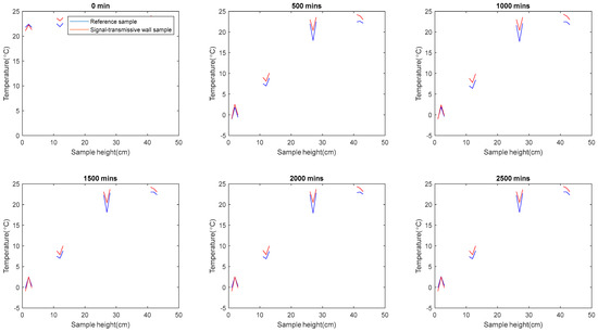
Figure 5.
Temperature profiles of two samples.
4.2. AI-Based Conductivity Predictor
The basic flowchart of our AI-based scheme is shown in Figure 6. In the practical measurement, the bottom concrete was considered as the exterior wall, which was exposed to a low temperature controlled by cooling thermostats. The other faces including the top surface (concrete) were open. As shown in Figure 7, the temperature sampling points were set in the model bottom, two intersections between different materials, and the center of the rock wool. With the temperature data acquired by thermal data logger, an HS-based AI method was developed to find the optimal thermal conductivity values so that the measured temperature profile could match that from the MATLAB simulations.
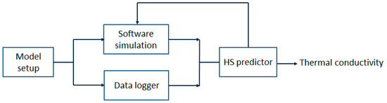
Figure 6.
The thermal conductivity estimation method.
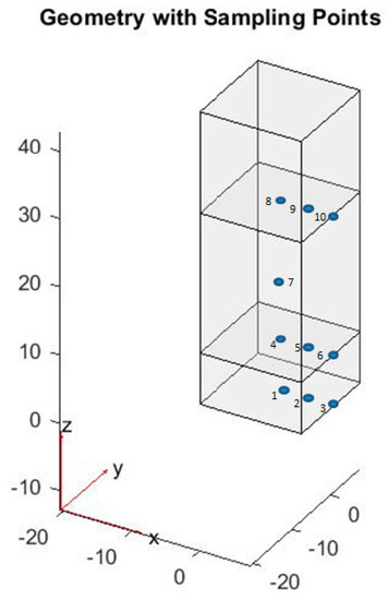
Figure 7.
Temperature sampling points.
There were ten temperature sampling points distributed in the model bottom, two intersections between different materials, and the center of sample, as shown in Figure 7.
In the simulations, the Partial Differential Equation (PDE) toolbox of MATLAB was used to evaluate the fitness of the candidates obtained by our HS algorithm, and the Dirichlet boundary condition was set on the model. Figure 8 shows the model at the initial state (room temperature) and the model with a triangular element mesh. Because of the type of thermal couples, Hmax in the PDE toolbox was set to be 0.1 in order to control the size of the triangles on the mesh. From the temperature sampling locations in Figure 7 obtained by the laboratory measurement, we could acquire the corresponding nodes in the PDE model as given in Table 2. Both the thermal performance comparison measurement and the PDE simulation results indicated that the surface temperatures on the top of the model were the same as those of the environment. There were two possible reasons. First, obtaining accurate surface temperatures with thermal couples was difficult since they were highly dependent on the ambient temperature. Second, the thickness of the model determining the top surface temperatures was not affected by the bottom cooling temperature. Thus, we only needed to consider ten sampling points as shown in Figure 7. It could help to reduce the computational burden in the MATLAB simulation. According to Table 2, the fitness function of our HS method is
where a, b, i, j, and T represent the simulation temperature, measurement temperature, number of sampling points, number of measurement (simulation) step, and measurement (simulation) time, respectively. The HS algorithm was applied to find the optimal solutions of the thermal conductivities of the concrete and rock wool, as well as the specific heats of the concrete and the rock wool by minimizing the above objective function.
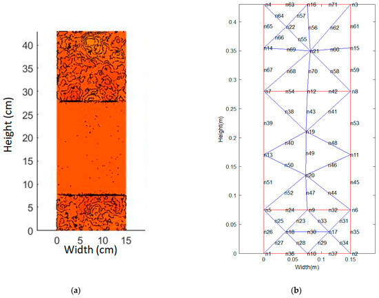
Figure 8.
(a) Model with initial state in room temperature. (b) Model with triangular element mesh.
Table 2.
The sampling points.
4.3. Harmony Search Algorithm
The field of AI has rapidly advanced during the recent years, and it has the potential to revolutionize numerous industries by making processes more efficient, improving decision-making, and enabling new types of products and services [24,25,26]. Actually, AI has been proved to be a powerful tool for optimization problems by analyzing tremendous amounts of data and identifying patterns [27,28]. The HS, inspired by the music improvisation process, is a metaheuristic global optimization method, which has gained great research attention and been widely used to handle different engineering problems [29,30]. When composing harmony, musicians typically experiment with various combinations of musical pitches that they have stored in the memory. This type of efficient search for a perfectly harmonious state is similar to the process used for finding the optimal solutions in engineering. Therefore, harmony improvisation has inspired the emergence of this novel type of Natural Inspired Computation (NIC) algorithm [31], the HS algorithm. Table 3 gives a comparison of the harmony improvisation and the optimization task [32]. Figure 9 shows the flowchart of the HS method involving four main steps as follows.
Table 3.
Comparison of optimization task and harmony improvisation.
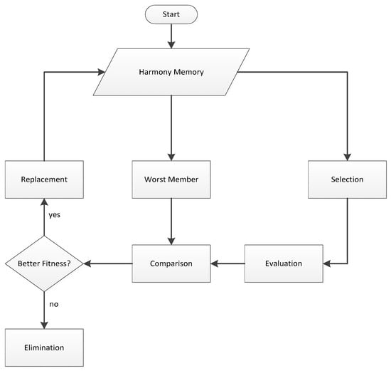
Figure 9.
Basic flowchart of HS algorithm.
Step 1. Initialize a candidate pool HS Memory (HM). The HM comprises a set of solutions generated randomly or based on prior knowledge to the given optimization problem that need to be solved. For a problem with the dimension of n, an HM with the candidate number of J can be represented as follows:
where () is a candidate solution. Note that storing past search experiences of HM plays an essential role in the optimization performance of the HS method.
Step 2. Generate a new solution based on the HM. Each component of this solution, , is obtained based on Harmony Memory Considering Rate (HMCR), which represents the probability of choosing a component from the HM. For example, when the HMCR is set to 1, it means that the new solution is randomly generated with 100% probability, rather than using the HM to select a component. If is from the HM, it is selected from the dimension of a random HM member. This component will be further changed with the consideration of the pitching adjust rate (PAR), which decides the probability of a candidate from the HM to be mutated. The improvisation process of is similar to the production of offspring in the Genetic Algorithm (GA) with the operators of mutation and crossover [33,34]. However, the GA usually creates new chromosomes by combining the genetic information of only one (mutation) or two (crossover) existing parent solutions, while the improvisation of new solutions in the HS method enables the utilization of all the HM candidates.
Step 3. Update the HM. The new solution obtained from Step 2 is evaluated using a fitness function. The new one will replace the worst candidate in the HM if it yields better fitness. Otherwise, it will be discarded and not stored in the HS.
Step 4. Repeat Step 2 to Step 3 until a stop criterion is met.
Similar to the GA and other NIC techniques, the HS method is a stochastic population-based search approach. It does not require any prior domain knowledge beforehand, such as the gradient information of the objective functions [17]. Nevertheless, different from other population-based techniques, it employs only a single search memory to evolve. Therefore, the HS algorithm has the distinguished advantage of computational simplicity because it imposes few mathematical requirements. However, it also has some inherent drawbacks, e.g., the balance of exploration and exploitation. In summary, its characteristics of correlation among variables and multi-candidate consideration contribute to its flexibility, making it well suited for solving diverse optimization problems in engineering [16,35].
To demonstrate the effectiveness of our HS method, a four-dimensional (the same number of variables as the conductivity predictor) sphere function within the search range [0, 1000] is used.
The sphere function is as follows:
In this function, the optimal solution is 0 with the solution ( = 0). Figure 10 illustrates the convergence procedure in 1000 generations. The parameters used in the HS method for both the benchmark function and the thermal conductivity predictor are given in Table 4. Apparently, the HS can converge significantly fast in this four-dimensional function optimization case.
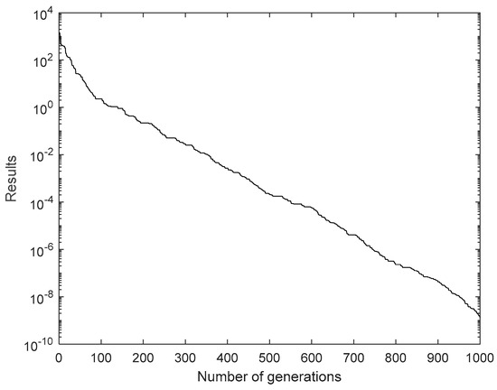
Figure 10.
Convergence of the HS in optimization of sphere function.
Table 4.
Parameters used in the HS method.
5. Results and Analysis
5.1. Results Based on Proposed HS Algorithms
As discussed previously, our measurement method employed the HS optimization algorithm to find the optimal values of the thermal conductivities by minimizing the objective function. The HS method works by iteratively refining the four-dimensional solution until a stopping criterion is met, which can be the qualified solution or a given number of iterations. Due to the characteristics of the HS algorithm, the maximum number of generations, 1000, was chosen as the stop criteria in our simulations. The convergence procedure is illustrated in Figure 11.
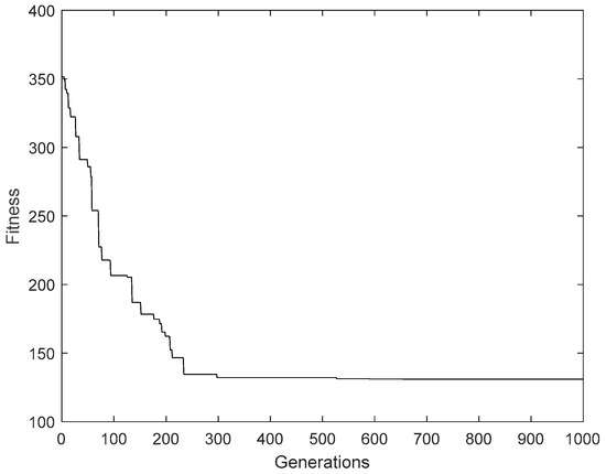
Figure 11.
Convergence procedure of the HS algorithm.
Table 5 provides the candidate parameters including the searching ranges and optimal values obtained by the HS algorithm. The optimal thermal conductivities of concrete and rock wool were 0.8961 and 0.104 (W/mK), respectively, which deviated from the theoretical values of 2 and 0.035 (W/mK) [19]. One possible explanation for this discrepancy was that the samples used for the measurements were handmade in a laboratory. Comprehensive simulation results indicated that for a large number of iterations, the convergence was independent of the searching ranges. In our sample, three thermal resistances were connected in series, and the total thermal resistance could be calculated by
Table 5.
Candidate information and optimal solutions.
The total thermal conductivity was
where l represents the thickness of the layer. Based on the above function, the total thermal conductivity () was 0.1935 W/mk, which was the same as that of the antenna-embedded sample.
We compared the temperature changes at the center of the intersection between the first concrete and rock wool layer until reaching the steady state, both in the measurement and in the simulations (point 4 in Figure 7). In Figure 12, there are 100 sampling intervals with the duration of 300 s between two intervals. Obviously, the values of the thermal conductivity and specific heat obtained by our proposed method were very close to the actual ones.
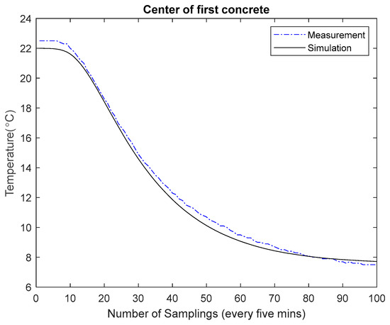
Figure 12.
Temperature changes of measurement and simulations at point 4 in Figure 7.
5.2. Analysis and Discussion
Figure 13 shows the MATLAB simulation of heat transfer based on the thermal property parameters of concrete and rock wool obtained through the proposed HS method (listed in Table 5). The 2D model had a width of 0.15 m, and layer heights were identical to those of the real sample. The temperature at the bottom edge of the model was set to −1 °C, which corresponded to the temperature measured at the bottom of our laboratory sample. The three subplots in Figure 13 illustrate the model temperature changes over the simulation time after 20, 40, and 600 min. Obviously, the temperature of the bottom layer changed rapidly and reached a stable state almost within 20 min, while the rock wool’s good thermal insulation enabled the temperature of the top layer to remain unchanged. This heat transfer simulation by MATLAB was almost consistent with the temperature profile displayed in Figure 5.
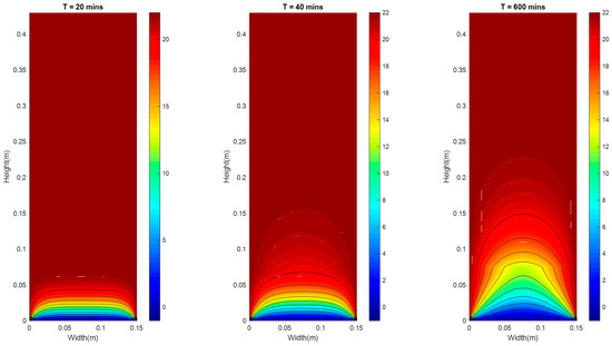
Figure 13.
Model in temperature change.
As previously mentioned, the HS method had the advantages of efficient search, robustness, and easy implementation. In the simulation, we also found that the optimized results were insensitive to the specified searching range. It indicated that the HS algorithm was suitable for predicting material thermal property parameters in cases where the real values were unknown. Our thermal property prediction model was based on measurement data, which may be subject to errors resulting from the accuracy of thermal data loggers. As given in the previous section, the accuracy of the two data loggers was ±0.5 °C, which could potentially influence the optimized results. The HS method was shown to be robust against these types of errors, making it appropriate for solving real-world engineering problems. Our proposed algorithm initialized with a five-member memory pool that could help to reduce the computational burden in MATLAB. However, the HS algorithm had a significant disadvantage in slow convergence, particularly after it reached a local optimum. As shown in Figure 11, the algorithm only improved fitness slightly after 300 generations. Through trial and error simulations, we found that the algorithm could not converge even after 10,000 iterations, with only a little improvement in fitness.
Our AI-based scheme has several advantages over conventional methods, including simplicity, no need for prior knowledge, and low cost. However, there are still some inherent limitations and drawbacks. For instance, the values of the predicted thermal properties highly depended on the accurate mapping from the positions of thermal couples to their corresponding mesh modes in the simulation model. Hence, the shape of the thermal couples was an essential issue in measurement setup. The difficulty of acquiring surface temperature meant that the sampling points should be placed inside the model. As a result, the proposed method was applicable to solid samples even with complex structures but not suitable for multilayer ones without low-density material in the middle layer.
6. Conclusions
The contradiction between the quality of life and the energy crisis promotes the study of new construction materials. The new signal-transmissive wall can handle the outdoor-to-indoor communication connectivity in 5G. However, the influence on thermal performance determines its feasibility, which is a very challenging issue. Limited by the size and inhomogeneous structure, the thermal conductivity measurement of wall samples becomes a demanding issue. On the other hand, the actual thermal property values of handmade laboratory samples are significantly different from those calculated in theory. With the steady-state methods, it is difficult to control the heat loss to ensure the heat flows in one direction, particularly in cases of large volumes of samples in laboratory measurements. Due to the complexity of the measurement setup and limitations in sample size and structure, it is hard to employ the transient state methods to yield satisfactory measurement results. Our paper presents a new thermal insulation assessment approach for the handmade samples in the laboratory, which has the remarkable advantages of low cost, robustness, and simplicity. In this AI-based scheme, the HS algorithm is utilized to find the optimal values of the thermal properties. Compared with the conventional schemes, it is relatively simple to set up and can be used to measure a wide range of solid material thermal properties regardless of thickness and structure. On the other hand, it does have some drawbacks including the accuracy limitation of thermal couples and premature issue of the HS method. In the future work, we will extend the applications to other thermal performance problems with more complex structures. However, this novel method also has some drawbacks, such as the sensitivity of the thermal couples under the experimental conditions and the potential errors caused by the heat losses not considered in the PDE model. How to overcome the shortcomings will be another potential research topic for us to investigate.
Author Contributions
Conceptualization, K.H. and L.V.-S.; methodology, X.W. and X.L.; software, X.W.; validation, X.W. and X.L.; investigation, X.L., X.W., K.H. and L.V.-S.; resources, K.H. and X.L.; writing—original draft preparation, X.W.; writing—review and editing, K.H., L.V.-S. and X.L.; supervision, X.L.; project administration, K.H. and X.L.; funding acquisition, K.H. and X.L. All authors have read and agreed to the published version of the manuscript.
Funding
This research received was funded by the Academy of Finland, project STARCLUB, grant number 324023.
Data Availability Statement
Data available on request from the authors.
Conflicts of Interest
The authors declare no conflict of interest.
References
- International Telecommunication Union. Available online: https://www.itu.int (accessed on 1 March 2023).
- Vähä-Savo, L.; Atienza, A.G.; Cziezerski, C.; Heino, M.; Haneda, K.; Icheln, C.; Lü, X.; Viljanen, K. Passive antenna systems embedded into a load bearing wall for improved radio transparency. In Proceedings of the 50th European Microwave Conference (EuMC), Utrecht, The Netherlands, 12–14 January 2021. [Google Scholar]
- Ntontin, K.; Verikoukis, C. Relay-aided outdoor-to-indoor communication in millimeter-wave cellular networks. IEEE Syst. J. 2020, 14, 2473–2484. [Google Scholar] [CrossRef]
- Er-reguig, Z.; Ammor, H. Towards designing a microcell base station using a software-defined radio platform. In Proceedings of the 2019 7th Mediterranean Congress of Telecommunications, Fes, Morocco, 24–25 October 2019. [Google Scholar]
- Vähä-Savo, L.; Koivumäki, P.; Haneda, K.; Icheln, C.; Chen, J. 3-D Modeling of Human Hands for Characterizing Antenna Radiation from a 5G Mobile Phone. In Proceedings of the 2022 16th European Conference on Antennas and Propagation, Madrid, Spain, 27 March–1 April 2022. [Google Scholar]
- Salmon, D. Thermal conductivity of insulations using guarded hot plates including recent developments and sources of ref-erence materials. Meas. Sci. Technol. 2001, 12, R89. [Google Scholar] [CrossRef]
- Flaata, T.; Michna, G.J.; Letcher, T. Thermal conductivity testing apparatus for 3D printed materials. In Proceedings of the Heat Transfer Summer Conference, Washington, DC, USA, 9–12 July 2017. [Google Scholar]
- Elkholy, A.; Sadek, H.; Kempers, R. An improved transient plane source technique and methodology for measuring the thermal properties of anisotropic materials. Int. J. Therm. Sci. 2019, 135, 362–374. [Google Scholar] [CrossRef]
- Asadi, I.; Shafigh, P.; Hassan, Z.F.; Mahyuddin, N.B. Thermal conductivity of concrete—A review. J. Build. Eng. 2018, 20, 81–93. [Google Scholar] [CrossRef]
- Llavona, M.A.; Zapico, R.; Blanco, F.; Verdeja, L.F.; Sancho, J.P. Methods for measuring thermal conductivity. Rev. Minas. 1991, 6, 89–98. [Google Scholar]
- Palacios, A.; Cong, L.; Navarro, M.E.; Ding, Y.; Barreneche, C. Thermal conductivity measurement techniques for characterizing thermal energy storage materials—A review. Renew. Sustain. Energy Rev. 2019, 108, 32–52. [Google Scholar] [CrossRef]
- Meshgin, P.; Xi, Y. Multi-scale composite models for the effective thermal conductivity of PCM-concrete. Constr. Build. Mater. 2013, 48, 371–378. [Google Scholar] [CrossRef]
- Zhao, D.; Qian, X.; Gu, X.; Jajja, S.A.; Yang, R. Measurement techniques for thermal conductivity and interfacial thermal conductance of bulk and thin film materials. J. Electron. Packag. 2016, 138, 040802. [Google Scholar] [CrossRef]
- Elkholy, A.; Kempers, R. An accurate steady-state approach for characterizing the thermal conductivity of additively manufactured polymer composites. Case Stud. Therm. Eng. 2022, 31, 101829. [Google Scholar] [CrossRef]
- Cahill, D.G. Thermal conductivity measurement from 30 to 750 K: The 3ω method. Rev. Sci. Instrum. 1990, 61, 802–808. [Google Scholar] [CrossRef]
- Lee, K.S.; Geem, Z.W. A new structural optimization method based on the harmony search algorithm. Comput. Struct. 2004, 82, 781–798. [Google Scholar] [CrossRef]
- Wang, X.; Gao, X.Z.; Zenger, K. An Introduction to Harmony Search Optimization Method; Springer International Publishing: New York, NY, USA, 2015. [Google Scholar]
- Vähä-Savo, L.; Haneda, K.; Icheln, C.; Lü, X. Electromagnetic-Thermal Analyses of Distributed Antennas Embedded into a Load Bearing Wall. arXiv 2022, arXiv:2207.06185. [Google Scholar]
- Lu, T.; Vähä-Savo, L.; Lü, X.; Haneda, K. Thermal Impact of 5G Antenna Systems in Sandwich Walls. Energies 2023, 16, 2657. [Google Scholar] [CrossRef]
- Aksöz, S.; Öztürk, E.; Maraşlı, N. The measurement of thermal conductivity variation with temperature for solid materials. Measurement 2013, 46, 161–170. [Google Scholar] [CrossRef]
- Assael, M.J.; Chen, C.F.; Metaxa, I.; Wakeham, W.A. Thermal conductivity of suspensions of carbon nanotubes in water. Int. J. Thermophys. 2004, 25, 971–985. [Google Scholar] [CrossRef]
- Guo, R.; Ren, Z.; Bi, H.; Xu, M.; Cai, L. Electrical and thermal conductivity of polylactic acid (PLA)-based biocomposites by incorporation of nano-graphite fabricated with fused deposition modeling. Polymers 2019, 11, 549. [Google Scholar] [CrossRef]
- Shemelya, C.; De La Rosa, A.; Torrado, A.R.; Yu, K.; Domanowski, J.; Bonacuse, P.J.; Martin, R.E.; Juhasz, M.; Hurwitz, F.; Wicker, R.B.; et al. Anisotropy of thermal conductivity in 3D printed polymer matrix composites for space based cube satellites. Addit. Manuf. 2017, 16, 186–196. [Google Scholar] [CrossRef]
- Rich, E. Artificial Intelligence; McGraw-Hill: New York, NY, USA, 1983. [Google Scholar]
- Spector, L. Evolution of artificial intelligence. Artif. Intell. 2006, 170, 1251–1253. [Google Scholar] [CrossRef]
- Bastani, F.; Chen, I. The Reliability of Embedded AI Systems. IEEE Intell. Syst. Appl. 2018, 8, 72–78. [Google Scholar] [CrossRef]
- Hashim, F.A.; Hussien, A.G. Snake Optimizer: A novel meta-heuristic optimization algorithm. Knowl.-Based Syst. 2022, 242, 108320. [Google Scholar] [CrossRef]
- Sharma, N.; Gupta, R.D.; Khanna, R.; Sharma, R.C.; Sharma, Y.K. Machining of Ti-6Al-4V biomedical alloy by WEDM: Investigation and optimization of MRR and Rz using grey-harmony search. World J. Eng. 2023, 20, 221–234. [Google Scholar] [CrossRef]
- Abdulkhaleq, M.T.; Rashid, T.A.; Alsadoon, A.; Hassan, B.A.; Mohammadi, M.; Abdullah, J.M.; Chhabra, A.; Ali, S.L.; Othman, R.N.; Hasan, H.A.; et al. Harmony search: Current studies and uses on healthcare systems. Artif. Intell. Med. 2022, 131, 102348. [Google Scholar] [CrossRef] [PubMed]
- Güven, A.F.; Yörükeren, N.; Samy, M.M. Design optimization of a stand-alone green energy system of university campus based on Jaya-Harmony Search and Ant Colony Optimization algorithms approaches. Energy 2022, 253, 124089. [Google Scholar] [CrossRef]
- Geem, Z.W.; Kim, J.H.; Loganathan, G.V. A new heuristic optimization algorithm: Harmony search. Simulation 2001, 76, 60–80. [Google Scholar] [CrossRef]
- Geem, Z.W. Music-Inspired Optimization Algorithm: Harmony Search. Available online: http://www.hydroteq.com/ (accessed on 1 March 2023).
- Poli, R.; Langdon, W.B. Foundations of Genetic Programming; Springer: Berlin, Germany, 2002. [Google Scholar]
- Mahdavi, M.; Fesanghary, M.; Damangir, E. An improved harmony search algorithm for solving optimization problems. Appl. Math. Comput. 2007, 188, 1567–1579. [Google Scholar] [CrossRef]
- Geem, Z.W.; Kim, J.H.; Loganathan, G.V. Harmony search optimization: Application to pipe network design. Int. J. Simul. Model. 2002, 22, 125–133. [Google Scholar] [CrossRef]
Disclaimer/Publisher’s Note: The statements, opinions and data contained in all publications are solely those of the individual author(s) and contributor(s) and not of MDPI and/or the editor(s). MDPI and/or the editor(s) disclaim responsibility for any injury to people or property resulting from any ideas, methods, instructions or products referred to in the content. |
© 2023 by the authors. Licensee MDPI, Basel, Switzerland. This article is an open access article distributed under the terms and conditions of the Creative Commons Attribution (CC BY) license (https://creativecommons.org/licenses/by/4.0/).