Article

Fault Detection in Distribution Network with the Cauchy-M Estimate—RVFLN Method

Electrical and Electronics Engineering Department, Faculty of Engineering, Dicle University, Diyarbakır 21280, Turkey
*
Author to whom correspondence should be addressed.
Energies 2023, 16(1), 252; https://doi.org/10.3390/en16010252
Submission received: 4 November 2022 / Revised: 1 December 2022 / Accepted: 6 December 2022 / Published: 26 December 2022

Abstract

:
Fault detection is an important issue in today’s distribution networks, the structure of which is becoming more complex. In this article, a data-based Cauchy distribution weighting M-estimate RVFLNs method is proposed for short-circuit fault detection in distribution networks. The proposed method detects short circuits based on current and voltage measurements. In addition, noises were added to the data to ensure the robustness of the method. The performance of the method was examined in the RTDS RTS simulator using the IEEE 33-bus-bar system model with the help of real-time simulations. The success rate of the proposed method is between 98% and 100% for low-impedance (0 ohm) short-circuit faults, depending on the fault type. The success rate of high-impedance (100 ohm) short-circuit faults, which are more difficult to detect, is between 80% and 92%, depending on the fault type.

1. Introduction

In general, power systems consist of three main parts. These are the generation systems where the electricity is produced, the transmission systems where the electricity is carried from the production sites, and the distribution systems where the users are connected to the grid [1]. Advanced technologies increase the power demand continuously and uninterrupted power systems are important to satisfy this demand. However, entirely uninterrupted power transmission is not possible. These power outages both cause energy losses in systems and harm the country’s economy. For instance, according to the Council of European Energy Regulator’s (CEER’s) report on power losses in 2020, 18 European countries had distribution losses ranging from 2% to 9% between 2012 and 2018 [2]. The Electricity Security report published in 2021 demonstrated that USA households suffered from an immediate cost of 1590 dollars per kW because of power outages [3]. Therefore, power outages should be quickly detected, classified and resolved. In power systems, 80% of faults occur in the distribution part [4]. Especially, distribution systems have become very complex, with the connection of renewable energy sources, electric vehicles and battery systems to them. Distribution networks are highly influenced by these new elements included. Due to this complex network structure, it becomes complex to detect the faults and difficult to locate them [5,6].
In the distribution networks, the outages are caused by different types of short-circuit faults which are classified as symmetrical and asymmetrical faults. The symmetrical fault that ensures the system’s stability is a three-phase (PPP) short-circuit fault. Although this fault has a low probability to occur, it is the most severe short-circuit fault since it damages the system equipment. Another fault type is asymmetrical faults that lead to instability in the power system. Asymmetrical faults include two-phase-to-ground faults (2PP-G), single phase-to-ground (1P-G) faults, and phase-to-phase (2P-P) faults. The faults that occur in distribution networks are generally 70% single-phase-to-ground faults, 15% two-phase faults, 10% two-phase-to-ground faults and 5% three-phase-to-ground faults [7,8,9].
Protection system fuses, automatic reclosers, and over-current relays are used to eliminate these failures in the distribution system [10,11,12]. Today, however, distribution systems are constantly evolving with the inclusion of wind energy systems, photovoltaic (PV) systems, biomass power plants and electric vehicles [6,13]. The traditionally passive nature of distribution systems turns into an active network with the continuous inclusion of new elements. This dynamic network structure brings it with many problems. These problems cause loss of protection coordination and the blinding of some relays [5,13]. It also causes severe damage to distribution networks due to high impedance fault (HIF) and low fault current magnitudes [5,14]. In particular, the high impedance fault (HIF) is below the limit that can be detected by over-current relays and fuses [15,16]. For example, [17], it is stated that commercial over-current relays can only detect 50% to 60% of cases despite efforts to develop devices to detect HIFs. Therefore, protection system fuses, auto-reclosers and over-current relays no longer meet the requirement for safe and stable operation every-time. A fast and accurate diagnostic method should be offered to increase the reliability of distribution systems, reduce economic losses, and shorten the time needed by maintenance personnel to search for faults.
Studies are available in the literature to resolve and classify faults. Fault detection is generally classified into two groups, which are model-based methods and pattern recognition methods. Model-based methods require a mathematical model that adequately explains the processing system. The complexity of calculations increases as the size of the power system network expands. The system fails to operate rapidly despite making an accurate classification [8,18,19]. Pattern recognition methods require a sufficient amount of historical process data. Intuitively, the task is defined with a set of mathematically expressible measurement data as a function between measurement and decisions. A mathematical expression of the underlying physical process is not required. Therefore, it leads to faster fault detection [8,18].
Fault detection with conventional machine learning classification methods has been vastly explored in the literature. In [20,21,22,23], a decision tree method was used for fault detection, but the method requires a great amount of training data and has a slow learning process. Fault detection was performed by using artificial neural networks (ANN) in [24,25,26,27,28]. However, this method is inefficient, as the training takes longer and causes such problems as over-fitting and under-fitting. In [29,30,31], support vector machines (SVMs) were used as the fault detection method whose sensitivity to parameter selection, however, is a disadvantage. As it is also a quadratics method, training times increase dramatically. Sparse Representation [32] was used as a fault detection method but it had disadvantages such as limited computational power in large data, classification with limited memory, and considerable slowness. In [33], although the Random Forest (RF) method was utilized for fault detection, it worked quite slowly in real-time estimations. Faults were detected with K-Nearest Neighbor in [34]. However, sensitivity to noise and outliers were among the observed problems. In [9,35], Extreme Learning Machine (ELM) was used for fault detection, but the conventional ELM fails to train large data rapidly and efficiently due to its memory residence and high space and time complexity. Fault detection was performed using Convolutional Neural Network (CNN) in [36,37]. Training CNNs takes a very long time, particularly with large data-sets. Special equipment (such as GPU) is usually needed to expedite the training process. In [38,39,40], fault detection was performed with the long short-term memory (LSTM) method. In LSTMs, easy over-fitting, longer training times, and sensitivity to random weight initialization are some of the drawbacks. A convolutional sparse auto-encoder (CSAE) was used in [41] for fault detection. As an automatic encoder learns to capture as much information as possible instead of the required information, certain important information may become lost, which is a disadvantage of this classification method.
Literature reviews have revealed that despite a large number of studies on short-circuit faults, very few studies are available on the detection of high-resistance faults. Including these studies, short-circuit fault detection studies generally disregarded the sensor-induced noises. In these studies, a novel method grounded on random vector functional link networks (RVFLN) for fault detection in the distribution network was proposed. This method worked by using current and voltage measurements. In order to test the performance and accuracy of the proposed method, an IEEE 33-bus power system was modeled in RTDS RTS (real-time simulator). In the resulting model, data were retrieved from different faults. In addition, the noise was added to these data to ensure robustness. In this study, 14 feature vectors were constructed from data considering both high-resistance short-circuit faults and sensor-induced noises in order to differentiate between fault conditions and normal operation. Such feature vectors were obtained from recorded current and voltage measurements. Then, the Cauchy Distribution Weighting M-Estimation RVFLNs (Cauchy-M-RVFLN) of the system was constructed. Finally, the detection performance of faults occurring in various types and resistances was explored with the trained Cauchy-M-RVFLN system. Results from the proposed method were contrasted with those from leading classification methods available in the literature. The contributions of this study are as follows:
1
In real-time studies, noise is an inevitable problem for sensors. If these noises in sensors are disregarded, they may cause such problems as declassification, low accuracy, and under-fitting in both signal processing and machine learning practices. Noise has been disregarded in many studies in the literature ([18,19,21,22,23,24,25,26,27,28,29,30,31,32,34,35,36,37,38,39,40]). This study, however, takes the noise effect into account.
2
Studies in the literature generally used Matlab for the implementation of the single-bus distribution systems. Matlab simulations must be compared with real-time systems or its stability analysis must be presented. In this proposed method, the 33-bus system was implemented by using RTDS RTS (real time simulator). It is significant to use the IEEE 33-bus system in that it is a small-scale but comprehensive structure that encompasses virtually all of the features of real-time smart distribution systems.
3
The proposed Cauchy M-RVFLNs, thanks to the calculation method for random layers and weights (non-use of LS), overcomes problems encountered by conventional methods such as back propagation and gradient descent, low accuracy with small datasets, long learning times, great need for computational sources, quadratic programs and noise sensitivity.
4
In [18,19,20,21,22,23,24,25,26,27,28,29,30,31,32,33,34,35,36,37,38,39,40], six previously unused novel features were constructed. These features contributed to the fault detection accuracy by 10% in high-resistance short-circuit faults.
5
In [18,19,20,21,22,23,24,25,26,27,28,29,30,31,32,33,34,35,36,37,38,39,40], high-resistance short-circuit faults were assessed with other types of faults, and an average accuracy ratio was provided. High-impedance faults were not generally detected separately in the studies. In this study, the detection accuracy of short-circuit faults with different fault resistances has been presented separately.
The remainder of this paper has been edited as follows: In Section 2, we presented feature extraction and model formulation of the Cauchy-M-RVFLN system. In Section 3, we provided information on the 33-bus system simulated in RTDS. Section 4 contained the experimental results and a statistical assessment of classification models. Finally, in Section 5, the results were discussed.

2. Proposed Fault Detection Method

We will demonstrate how to construct new feature vectors grounded on the voltage and current measurements of 33-bus system which was modeled in the RTDS simulator. For real-time fault detection, the Cauchy-M-RVFLN model is proposed. In this model, the Cauchy M estimate RVFLN method proposed by [42] for the estimation of molten iron quality in iron production facilities is used. However, the Cauchy M RVFLN method has not been used for fault detection in distribution systems. In this study, the success of this method in fault detection has been examined.

2.1. Feature Construction

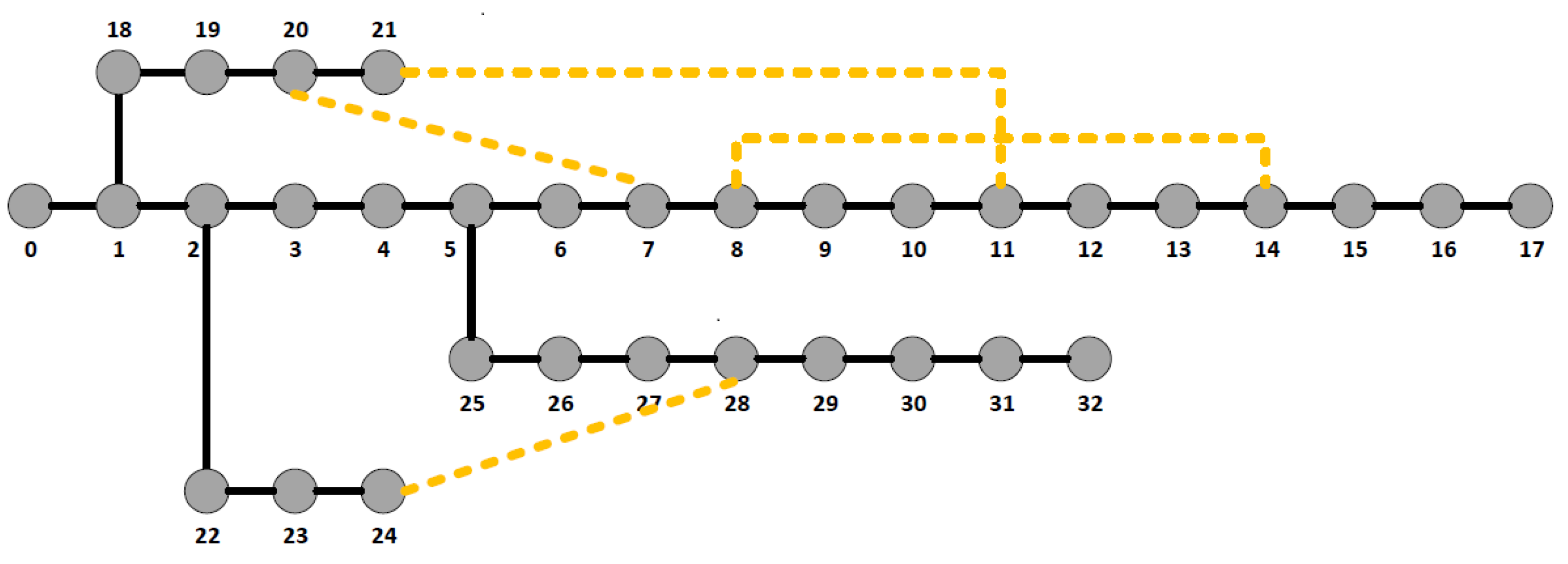
Data must be prepared to detect the faults in a power system and differentiate faults from normal system operation. In the IEEE 33-bus power system modeled in RTDS, current and voltage data are retrieved from eight different buses n = 7, 8, 11, 14, 20, 21, 24, and values are measured from each phase in these buses. Feature vectors were constructed from these measured values. A total of 14 feature vectors listed in Table 1 were constructed to contain different fault conditions. The initial four feature vectors (F1, F2, F3, and F4) were used as current magnitude In( φ i)t, voltage magnitude Vn( φ i)t, current angle θ In ( φ i)t, and voltage angle θ Vn ( φ i)t, respectively, to secure the applicability of the recommended algorithm to power systems of different sizes and to abstain from parameter re-setting [43]. F5, F6, F7, and F8 serve to detect the immediate changes in current and current angle and the immediate changes in voltage and voltage angle. F9, F10, F11, F12, F13, and F14 raw measured data can be transformed into differential features through signal norms. The appropriate signal attributes are achieved with three main signal norms, which are norms 1, 2, and infinity [44]. We calculated the 1-norm, 2-norm, and infinity norm (1, 2 and ℓ∞-norms, respectively) for each row of the feature matrix to obtain vectors.

2.2. RVFLN’s Model Establishment

The RVFLN Model was developed by Pao et al. as a single hidden layer feedforward network in 1992 [45]. Its simple structure is shown in Figure 1. RVFLN has been successfully used in several engineering techniques [42,46,47,48,49,50] for regression and classification purposes since its development. The advantage of RVFLN is that the weights between the input layer and the hidden layer are randomly appointed and do not need to be adjusted. The output weights are calculated using the least squares method algorithm (LS). RVFLNs can process the data in real time in most technical procedures.
a x = [ a 1 , a 2 , , a x n ] T R n and b x = [ b 1 , b 2 , , b x m ] T R m can be, respectively, defined as input and output vectors, and L can represent the hidden-node RVFLNs:
f L , x ( a x ) = j = 1 L ψ j v ( < z j , a x > + p j ) x = 1 , 2 , , M
f L , x ( a x ) is the output of RVFLNs, z j R n , j = 1 , , L is the hidden weighting matrix that is randomly generated in a certain probability space and links the input layer to the hidden layer [42,48], ψ j = [ ψ j 1 , ψ j 2 , , ψ j m ] T jth are the output weights that link the hidden node to training output nodes, p j is the bias of hidden node jth < z j , a x > z j , a x denotes the inner product of vectors, and v ( · ) is a non-linear activation function that satisfies one of the following equations.
R v 2 ( a ) d a < or R [ v ( a ) ] 2 d a <
Minimizing the error between actual output values and modal output values is essential for the learning purpose of RVFLNs. That is, it needs to find ψ j , z j and p j that satisfy the following conditions.
j = 1 L ψ j v ( < z j , a x > + p j ) = b x , x = 1 , 2 , , M
which can be composed exactly as
D ψ = B
D is the hidden output matrix, ψ represents the training output weighting matrix and B is intended as the output matrix, which are particularly identified as:
D ( z 1 , , z L , a 1 , , a M , p 1 , , p L ) = D 1 D M
= v ( < z 1 , a 1 > + p 1 ) v ( < z L , a x > + p L ) v ( < z 1 , a M > + p 1 ) v ( < z L , a M > + p L ) M x L
Description 1.Random parameter intervals ( z j , p j ) should be chosen appropriately for the performance of RVFLNs. In [48], Igelnik and Pao came up with a theoretical conclusion to determine random parameter ranges. Because the parameters are estimated by trial and error, it is still difficult to use the theoretical result proposed in [42,48] in real applications. In this study, we will adjust parameter ranges from [ 1 , 1 ] to [ M , M ] based on the experimental results, where M Z + .
Parameters ( z 1 , , z L , p 1 , , p L ) are randomly assigned to train the functionally linked networks and detect the weight of the optimal outputs ψ ^ :
ψ ^ = arg min ψ R L x m D ψ B 2
The solution LS is implemented, ψ ^ = D B and D = ( D T D ) 1 D T is the generalized Moore–Penrose inverse of the matrix D . Furthermore, the private solution ψ ^ = D B has the least norm. All of them are the LS solutions of D ψ = B .

M-Estimation-Robust RVFLNs Algorithm

The M-estimation suggested by Huber is the most widely used robust estimation method [42,51,52,53,54,55]. Unlike LS, which uses the sum of squared differences between noticed and calculated values as the objective function, M-estimation identifies a new objective loss function for the residual error. The recommended RVFLNs algorithm with M-estimation (M-RVFLNs) is identified as follows.
(1)
One-Output M-RVFLNs:
m = 1 , ψ , B in (4) can be simplified as
ψ = [ ψ 1 , ψ 2 , , ψ L ] L × 1 T , B = [ b 1 , b 2 , , b L ] M × 1 T
Thus, the LS solution of (4) is given as ψ ^ = D B = ( D T D ) 1 D T and the corresponding objective function is:
Q = x = 1 M r x 2 = x = 1 M ( b x D x ψ ) 2
After the introduction of M-estimation for RVFLNs, the objective function of the modeling residuals is changed to:
Q = x = 1 M ρ ( r x ) = x = 1 M ρ ( b x D x ψ )
where ρ is an influence function of the residuals. The optimal outputs weight link ψ ^ of M-RVFLNs can be determined as follows:
ψ ^ = arg min ψ x = 1 M ρ ( b x D x ψ ) = arg min ψ x = 1 M ρ ( r x ( ψ )
When the robust scale estimator σ ^ is introduced to (11), the form of ψ ^ can be expressed as follows:
ψ ^ = arg min ψ x = 1 M ρ ( b x D x ψ σ ^ ) = arg min ψ x = 1 M ρ ( r x ( ψ ) σ ^ )
Let ( x = 1 M ρ ( r x ( ψ ) σ ^ ) ) / ψ = 0 one can acquire
x = 1 M φ ( r x ( ψ ) σ ^ ) D x T x = 1 M ρ ( r x ( ψ ) σ ^ ) D x T = 0
Define the following weight factor:
ω ( r x ) φ ( r x ) / r x
If we solve the estimation equation shown in (13)
x = 1 M ω ( r x ( ψ ) / σ ^ ) × ( b x D x ψ ) D x T = 0
This can be written precisely as
D T W D ψ = D T W B
The iteration formula of ψ ^ can be derived further:
ψ ^ ( k + 1 ) = ( D T W ( k ) D ) 1 D T W ( k ) B
W is the weighting matrix with ω x , x = 1 , 2 , , T as the diagonal elements, that is, W = d i a g w x , and each ω x is the weighting factor defined in (14).
Description 2.The robust scale estimator σ ^ in (12) is of great importance for M-estimation. σ ^ is determined as the median absolute deviation (MAD) around the median:
σ ^ = M A D / 0.6745 , M A D = m e d i a n i ( r i m e d i a n ( r i ) )
The statistical measure of dispersion that is less affected by the outliers in the dataset than the standard deviation is defined as the MAD. The square of the distances from the mean is obtained using the standard deviation. In this way, outliers can further influence the model established for greater weightings of large deviations. MAD works better with the Cauchy distribution [51].
(2)
Multi-Output M-RVFLNs:
m > 1 , M-RVFLNs have multiple outputs. Thus situated, ψ , B are clarified as:
ψ = [ ψ j 1 , , ψ j c , , ψ j m ] = ψ 11 ψ 1 m ψ L 1 ψ L M L × m , j = 1 , , L c = 1 , , m
and
B = [ b x 1 , , b x c , , b x m ] = b 11 b 1 m b M 1 b M m M × m , x = 1 , , M c = 1 , , m
The size of the weight factor matrix ω ( r x ( ψ ) / σ ^ ) and B are consistent, both are M × n sized, so that
ω = w 1 ω x h ω x m = ω 11 ω 1 m ω M 1 ω M m M × m
The estimation equation explained in (15) cannot be formed in matrix form as in (16), and the ψ ^ iteration formula becomes
ψ ^ ( k + 1 ) = [ ψ ^ j 1 ( k + 1 ) , , ψ ^ j h ( k + 1 ) , , ψ ^ j m ( k + 1 ) ] = [ ( D T W x 1 ( k ) D ) 1 D T W | x 1 ( k ) b x 1 , , ( D T W x h ( k ) D ) 1 D T W | x h ( k ) b x h , , ( D T W x m ( k ) D ) 1 D T W | x m ( k ) b x m ]
W = d i a g w x h c = 1 , 2 , , m . The application of multi-output M-RVFLNs can be described as follows:
Step 1: ψ ^ ( 0 ) is calculated by ψ ^ = D B = ( D T D ) 1 D T B ;
Step 2: The residual vector r ( 0 ) is calculated according to ψ ^ ( 0 ) ; afterwards, σ ^ is calculated by σ ^ = m e d i a n x ( r x m e d i a n ( r x ) ) / 0.645 to acquire the standardized residual vector ( r ^ ) ( 0 ) / σ ^ ( 0 ) ;
Step 3: Substitute the standardized residuals into the weighting ω ( r x ) φ ( r x ) / r x , to calculate each weighting factor, and also obtain the weighting matrix W ( 0 ) ;
Step 4: The ψ ^ ( 0 ) , ψ ^ ( k ) , ψ ^ ( k + 1 ) is calculated iteratively [34]. If predictions of all the parameters are smaller than the particularized convergence conditions ( ψ ^ j h ( k + 1 ) ψ ^ j h ( k ) / ψ ^ j h ( k ) < ϵ = 10 6 ), the final regression coefficients can be achieved as ψ ^ M = ψ ^ ( k + 1 ) .

2.3. Cauchy Distribution Weighting M-RVFLNs

The M-RVFLN evaluates the contribution of each observation to the estimator by weighting the outliers. Therefore, it is very important to decide on the weighting factor. Outliers should be determined accordingly. In addition, the weighting method of the Cauchy distribution is used in practical applications to solve the overfitting problems of conventional methods and the problems in the selection of harmonic parameters.
(1)
Definition of the Cauchy distribution method [56,57]:
The method of Cauchy distribution is the distribution that can be expressed virtually to the stability and probability density function (PDF). A random variable set D has Cauchy distribution if D has a perpetual distribution on R and its PDF is:
p ( d ; h c , k c ) = k c / π ( k c 2 + ( d d c 2 ) ) , d R
h c R , is the parameter specification of the location of the summit of the distribution, and k c ( 0 , ) It is explained as the scale parameter that gives half the width at half maximum. Precisely, the max value of the Cauchy PDF is 1 / π k c , which is at d = h c The farther d is from h c , the smaller the value of p ( d ) .
(2)
Parameter determination method:
The feature of Cauchy distribution is emphasized by parameters k c and h c :
1.
h c : is used to determine the roles of “outliers” and h c is the median value of the modeling error ( h c = m e d i a n ( r x ) ).
2.
k c : As shown in (39), Cauchy describes the characteristic of the PDF, its value needs to be designated by the statistical properties of the modeling error distribution. If the modeling error distribution is small, the value of k c should be huge. Otherwise, k c must be small. It can be explained as a function of the inverse of the standard deviation of the k c modeling error. Equation (24) explains:
k c = 1 x = 1 M r x x = 1 M r x M 2 / M
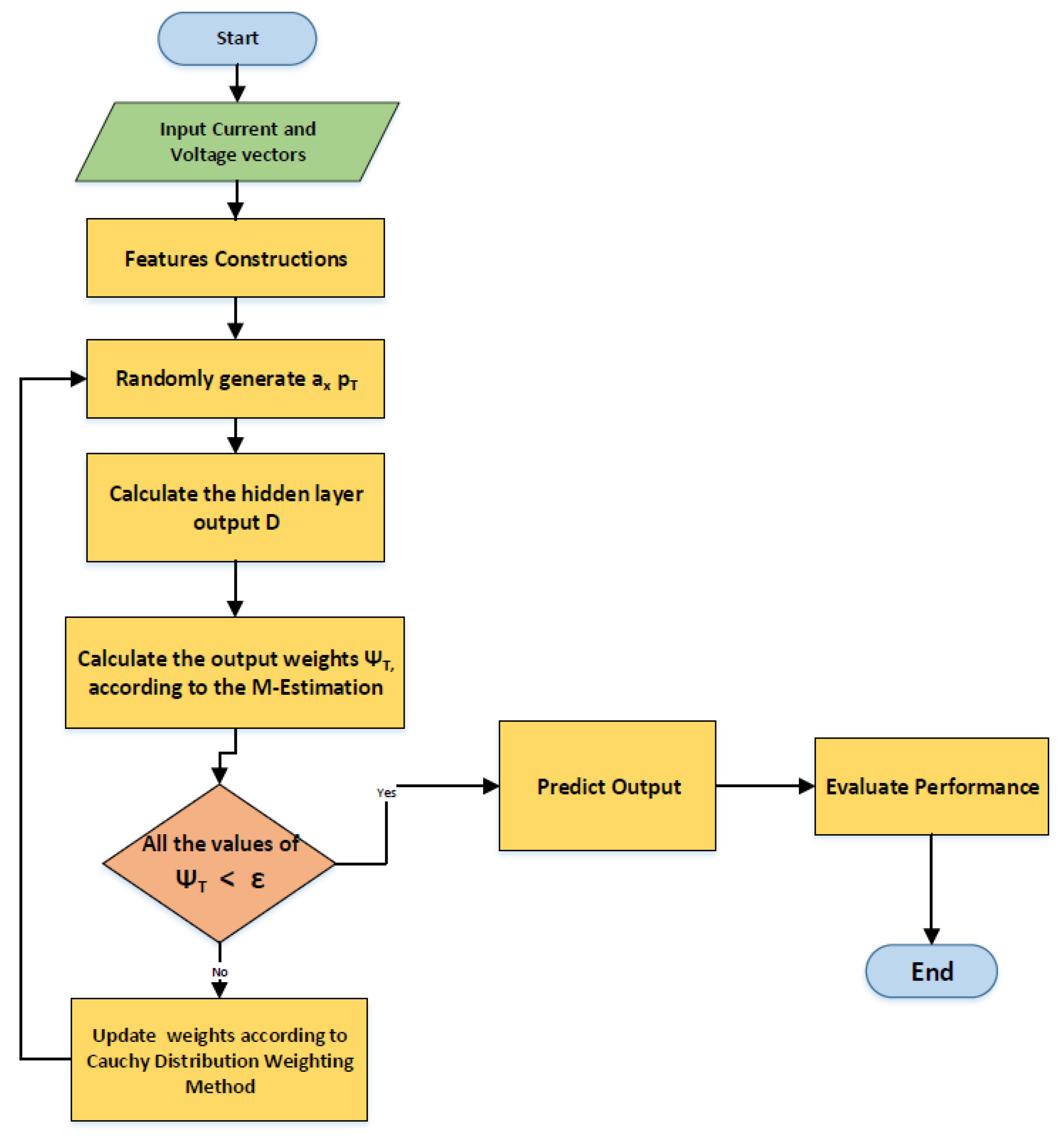
The flow chart of the proposed method is given in Figure 2. First, the properties were obtained from the current and voltage vectors taken from the system. Then, the initial weights of the RVFLN algorithm were randomly initialized. D was then calculated. Output weights were calculated using the M-estimate method. The weights are updated according to the Cauchy Distribution Weighting method until the condition in Step 4.

3. Case Studies

As a result of the introduction of energy sources into power systems, such as distributed generators, renewable energy systems, distributed storage, and electrical equipment, power systems have become more complex. Therefore, an expanded testing scale is required for power system studies. The IEEE 33-bus system developed by Baran and Wu [58] is a small but comprehensive structure that encompasses virtually all features of real-time intelligent distribution systems. The IEEE 33-bus distribution test system is shown in Figure 3. The IEEE 33-bus radial distribution system consists of thirty-three buses and thirty-two lines. All bus-bars operate at a 12.66 kV voltage level. The maximum and minimum voltage limits for all bus-bars are considered ± 5 % . The network has a total power of 3.715 MW and 2.3 MVAR connected to thirty-two bus-bars with different power factors. More detailed information can be found in the articles [59,60,61,62]. The IEEE 33-bus system represents an advanced benchmark for modern power distribution networks and is suitable for research needs with its suitable reactive power compensation units, integration of one-phase generation, storage units, balanced and unbalanced three-phase versions.
In this study, the IEEE 33-bus system shown in Figure 3 was preferred because it is a small but comprehensive structure that includes virtually all the features of intelligent real-time distribution systems. Real-Time Digital Simulation Software (RTDS) is used to apply new ideas and test existing ones before power system equipment is connected to real systems. The Real-Time Simulation Software Package (RSCAD) simulation interface using RTDS is designed for power system simulation. It contains a large number of power system components in its library to simulate the RSCAD power system. Thus, it is possible to create, control and analyze power systems and microgrids in real time [63,64]. The IEEE 33-bus power distribution system was modeled in RSCAD simulation software. Then, current and voltage data were retrieved from eight different buses n = 7, 8, 11, 14, 20, 21, 24, and values are measured from each phase in these buses. Fault data, including three single-phase ground fault (PG), three two-phase faults (PP), two two-phase ground faults (PP-G), and three three-phase faults (PPP), were obtained considering the parameters in Table 2.

4. Real-Time Simulation Results and Discussion

Modern power and energy systems are characterized by distribution, transmission, generation, storage, the massive integration of electrical equipment, and the interconnection of renewable energy systems and consumers, resulting in an extremely complex structure. In such a complex environment, advanced testing and validation methods are required to efficiently validate the power systems and controls to support the transition to a clean and sustainable energy system [65]. In the past, modeling was performed using traditional phasor-based approaches. However, since phasor-based modeling tools are not able to represent low-level inverter controls or capture the fast network dynamics during transient conditions, good results could not be obtained. For modern power systems, EMT simulators are increasingly preferred due to their ability to provide results over a wide frequency range. In the present study, we used the RTDS (Real-Time Digital Simulator or RTS), which was a real-time simulator originally developed in the 1980s [66,67].

4.1. Simulation Results

In this study, the IEEE 33-bus system model is simulated the RTDS Simulator. Fault data with different fault resistances were obtained in this model. Then, fault types were classified using these simulation data with the Cauchy-M-RVFLN Algorithm method. As seen in Table 3, accuracy decreased as fault resistance increased. The method achieved the lowest accuracy with 82% for a two-phase fault in 100 ohm fault resistance.

4.2. Robustness Simulation Results

In this study, the proposed method’s reaction was tested by adding different proportions of outliers to the constructed datasets. Firstly, random samples in proportions of 0%, 5%, 10%, 15%, …, 50% were taken from the datasets acquired from the IEEE 33-bus system. Then, outliers were obtained by preprocessing the target output. Outliers were introduced to the target output B & = [ b 1 , , b 4 ] of these selected normal samples, as shown in the following equation:
b x , o u t l i e r = b x + s i n g × [ r a n d ( 0 , 1 ) ( m a x ( b x ) m i n ( b x ) ) ]
r a n d ( 0 , 1 ) are random values ranging from (0,1). m a x ( b i ) and m i n ( b i ) re explained as the maximum and minimum values of b i , respectively, under normal operating conditions. To make the outliers more unbalanced in practical applications, the ratio of positive to negative outliers in selected sample points is adjusted at a ratio of 2 to 1. Additionally, when adding the positive outliers, the sign should be = 1, when adding the negative outliers, the sign should be = −1. Unlike the training dataset, no outliers are added to the test dataset. Datasets from the IEEE 33-bus system were used to test the robustness of the recommended method against outliers. In addition, 20% of the samples were elected from the normal training dataset, and the target output of these selected samples was preprocessed with the formula:
b x , o u t l i e r = b x + α × s i n g × [ r a n d ( 0 , 1 ) ( m a x ( b x ) m i n ( b x ) ) ]
α = ranges from 0 to 5 in increments of 0.5 and serves to calculate the amplitudes of outliers. Likewise, the ratio of outliers with positive and negative trends in selected sample points is adjusted at a ratio of 2 to 1 to make the outliers more unstable. In addition, the test data set does not contain any outliers.
In the present study, new datasets were generated by adding outliers as described to the data previously processed in RTSD. The results of error classification accuracy using the Cauchy-M-RVFLN algorithm are shown in Table 4. As shown in Table 4, very similar results were found for noisy and noise-free data in the classification accuracy of the different types of errors at different error resistances. The accuracy of the method decreased by about 2% under noisy conditions. However, the accuracy of the method was high despite the added noise, which shows that the method provides accurate results despite the noise and proves its accuracy.

4.3. Comparison with Common Machine Learning Methods

In this study, we generated new datasets as described by adding outliers to data previously prepared in RTDS. According to this new dataset, the fault detection accuracy of conventional machine learning methods CNN, LSTM, SVM, ELM, RVFLNs and Cauchy-M-RVFLN used to detect faults in a distribution network was compared.
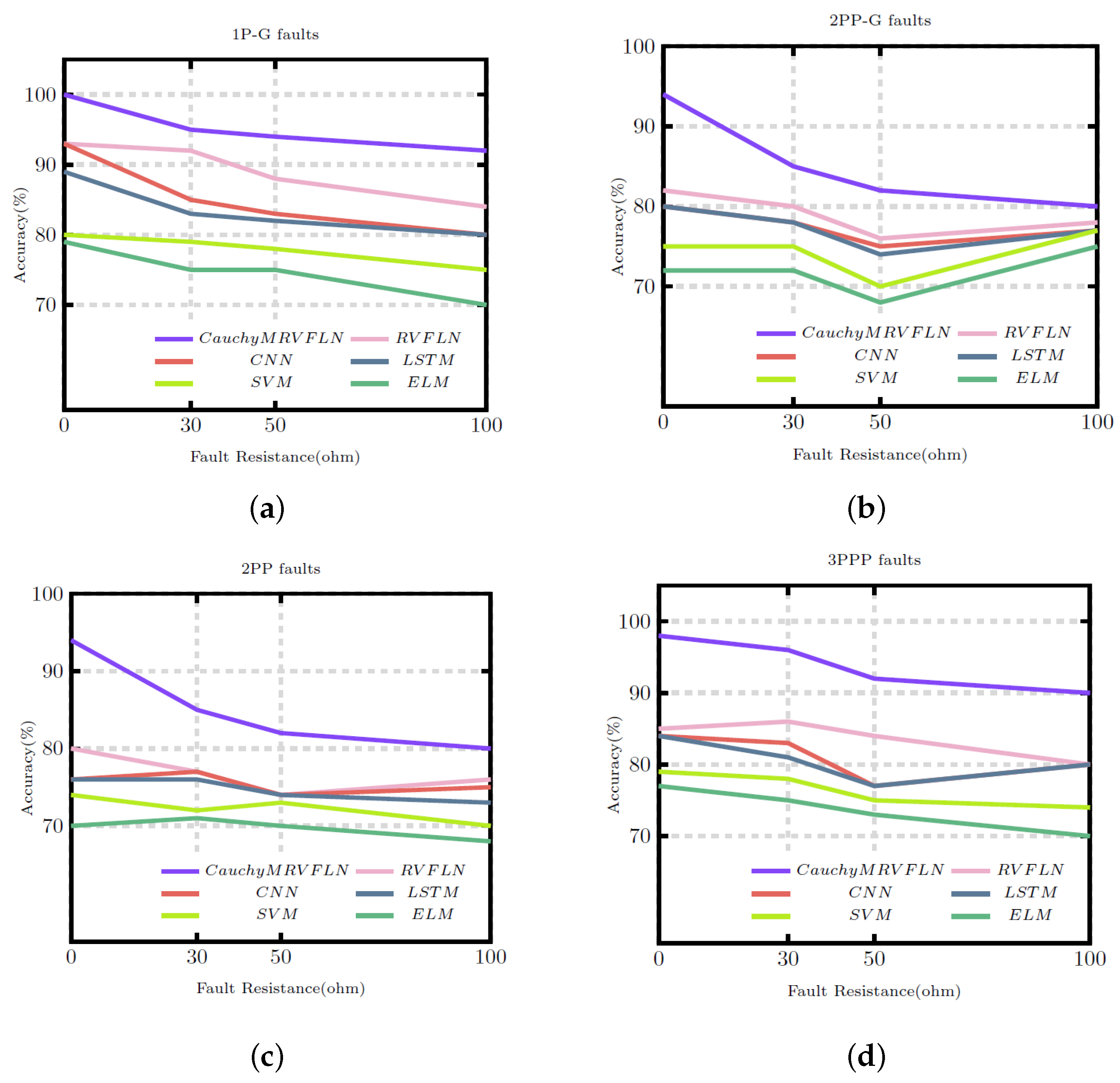
Figure 4 shows the fault detection accuracy of different methods for four different fault types with different fault resistances. As seen in Figure 4a, the highest accuracy in single phase-to-ground noise data was achieved with Cauchy-M-RVFLN. In case of a fault, the accuracy decreased as the fault resistance increased, but this method’s accuracy was high. The Cauchy-M-RVFLN method achieved 100% accuracy in 0 ohm fault resistance and 92% accuracy in 100 ohm fault resistance. The RVFLN method achieved 93% accuracy in 0 ohm fault resistance and 84% accuracy in 100 ohm fault resistance. The CNN method achieved 93% accuracy in 0 ohm fault resistance, which was the second best result, and 80% accuracy in 100 ohm fault resistance, which was lower than that of the RVFLN method. LSTM, SVM and ELM methods ranked 4th, 5th and 6th in terms of accuracy, respectively.
The highest accuracy was achieved with the Cauchy-M-RVFLN method in noise data with two phase-to-ground faults (Figure 4b). The Cauchy-M-RVFLN method performed fault detection with 94% accuracy in 0 ohm fault resistance, while the RVFLN method, which produced the closest results, detected the faults with 82% accuracy. The Cauchy-M-RVFLN method performed fault detection with 80% accuracy in 100 ohm fault resistance, while the RVFLN method, which had the closest results, detected the faults with 78% accuracy. For this fault type, fault classification accuracy was the highest with CNN, LSTM SVM and ELM methods, respectively, following the said two methods.
The highest accuracy was achieved with the Cauchy-M-RVFLN method in noise data with two-phase faults (Figure 4c). The Cauchy-M-RVFLN method performed fault detection with 94% accuracy in 0 ohm fault resistance and 80% accuracy in 100 ohm fault resistance. The Cauchy-M-RVFLN method performed the classification with 14% higher accuracy than the RVFLN method, which achieved the closest classification accuracy. CNN, LSTM, SVM and ELM methods had accuracy below 80%.
The highest accuracy was achieved with the Cauchy-M-RVFLN method in noise data with three-phase faults (Figure 4d). The Cauchy-M-RVFLN method performed fault detection with 98% accuracy in 0 ohm fault resistance and 90% accuracy in 100 ohm fault resistance. The RVFLN method achieved 85% accuracy in 0 ohm fault resistance and 80% accuracy in 100 ohm fault resistance. CNN and LSTM methods achieved 84% accuracy in 0 ohm fault resistance and 80% accuracy in 100 ohm fault resistance. SVM and ELM methods demonstrated an accuracy ratio below 80%. In all fault types and all fault resistance values, the Cauchy-M-RVFLN method had higher classification accuracy than the other compared methods. The accuracy decreased as the fault resistance increased, but this method’s accuracy was still high. The method delivered a classification performance with approximately 10% higher accuracy than the RVFLN method, which achieved the closest classification accuracy.

4.4. Comparison of Computational Efficiency

As given in Table 5, noise-added data were compared in CNN, LSTM, SVM, RVFLNs and Cauchy-M-RVFLN in terms of fault detection, training time and testing time. Although the training time of the proposed method was lower compared to RVFLN, the accuracy was high.

5. Comparison with Previous Studies

The proposed method was compared with other studies in the literature. As shown in Table 6, this study is more valuable than other publications due to the use of 14 different data inputs. In addition, the proposed method used a IEEE 33-bus system, while a single-bus system was utilized in most of the systems to generate simulation data. Studies in the literature were based on simulation data, but our study was conducted on a real-time simulator (RTDS). While most of the publications disregarded the noise values, this study also included the noise data. Considering all these parameters, we can say that this study stands out as it simulated real systems and demonstrated high accuracy.
In this paper, fault types in distribution systems were detected and classified by using the Cauchy-M-RVFLN method. Different from other studies in the literature, this study provided classification accuracy for each fault resistance. In the literature, an average classification success result is given for all fault resistance values. No studies were available that included high fault resistance values. In case of faults with high resistance, fault detection becomes more difficult, and the accuracy of methods decreases in high resistance values.
Studies in the literature, on the other hand, were conducted for zero or low fault resistances. Even though it may seem that studies in the literature had successful results, these achieved results were only for faults with 0 or low resistance. In the present study, accuracy was assessed separately for each fault resistance. In the table above, we proposed a total of 14 features, six of which were not in the literature. The classification was performed according to these features. A 33-bus system was modeled in RTDS to experiment with the method and retrieve data. In the model, data were obtained in realistic working conditions by taking modern distribution systems into consideration. The real-time nature of the model increased its accuracy. Sensor-induced noise was generally not considered in studies on the detection of short-circuit faults. In studies [20,30,51], the noise was taken into account. However, in these studies, single-bus systems were used. In the present study, results were obtained on a realistic model by considering both high-resistance short-circuit faults and sensor-induced noises.

6. Conclusion and Future Works

In this paper, data were obtained for three single-phase-to-ground faults, three two-phase-to-ground faults, three phase-to-phase faults and one three-phase short-circuit faults in 0 ohm, 10 ohm, 50 ohm and 100 ohm short-circuit fault resistances in the IEEE 33-bus power system modeled in RTDS. The Cauchy-M-RVFLN method was presented for the detection of short-circuit faults with different types and resistances. In order to test the method’s accuracy, data obtained from the system modeled in RTDS were used. Moreover, random noise was added to achieve more realistic data. Six new features were constructed for the detection of short-circuit faults with high fault resistances. These features contributed to increasing the detection accuracy of high-impedance short-circuit faults by 10%. In the classification based on data retrieved from RTDS, a classification accuracy of over 90% on average was achieved for all types of faults and resistances. It was observed that the accuracy slightly decreased as the fault resistance increased during a fault condition. In a later classification with added noise to simulation data, the accuracy decreased by 2%. In this study conducted with a multiple-bus real-time simulator, the success rate was high considering different types of faults and resistances. In the second section of this paper, comparisons were made with similar studies using different classification algorithms. Noise-added simulation data were used in this comparison. It was detected that the Cauchy-M-RVFLN method demonstrated very high accuracy results in different fault conditions. In addition, the proposed method had much higher training and testing speeds than other methods.
Since the features are normalized in the proposed algorithm, it can be successfully applied to transmission systems. The algorithm we propose provides both the short-circuit fault detection of transmission lines and the detection of high-impedance short-circuit faults that are difficult to detect. In addition, these fault types should be analyzed in order to use the proposed method in the detection of transformer and generator faults. The use of these recommended features in transformer and generator failures will provide a lower success rate compared to distribution and transmission networks. Therefore, it is necessary to extract new features for transformer and generator fault detection.

Author Contributions

Conceptualization, C.H. and B.G.; methodology, C.H. and B.G.; software, C.H.; validation, C.H. and B.G.; formal analysis, C.H.; investigation, C.H.; resources, C.H.; data curation, C.H.; writing—original draft preparation, C.H.; writing—review and editing, C.H. and B.G.; visualization, C.H.; supervision, B.G. All authors have read and agreed to the published version of the manuscript.

Funding

This research received no external funding.

Data Availability Statement

Not applicable.

Acknowledgments

This research is supported by the Research Projects Committee of Dicle University (DUBAP) with the project numbers MUHENDISLIK.20.002 and MUHENDISLIK.20.009. We are grateful to DUBAP for the support.

Conflicts of Interest

The authors declare no conflict of interest.

References

  1. Morais, J.; Pires, Y.; Cardoso, C.; Klautau, A. An Overview of Data Mining Techniques Applied to Power Systems. In Data Mining and Knowledge Discovery in Real Life Applications; Ponce, J., Karahoca, A., Eds.; IntechOpen: Rijeka, Croatia, 2009; Chapter 26. [Google Scholar]
  2. Council of European Energy Regulators. 2 nd CEER Report on Power Losses; CEER Publishing: Brussels, Belgium, 2020; Available online: https://www.ceer.eu/documents/104400/-/-/fd4178b4-ed00-6d06-5f4b-8b87d630b060 (accessed on 12 September 2022).
  3. IEA. Analytical Frameworks for Electricity Security. 2021. Available online: https://www.iea.org/reports/analytical-frameworks-for-electricity-security (accessed on 12 September 2022).
  4. Gholami, M.; Abbaspour, A.; Moeini-Aghtaie, M.; Fotuhi-Firuzabad, M.; Lehtonen, M. Detecting the location of short-circuit faults in active distribution network using PMU-based state estimation. IEEE Trans. Smart Grid 2019, 11, 1396–1406. [Google Scholar] [CrossRef]
  5. Nsaif, Y.M.; Lipu, M.H.; Ayob, A.; Yusof, Y.; Hussain, A. Fault Detection and Protection Schemes for Distributed Generation Integrated to Distribution Network: Challenges and Suggestions. IEEE Access 2021, 9, 142693–142717. [Google Scholar] [CrossRef]
  6. Silos-Sanchez, A.; Villafafila-Robles, R.; Lloret-Gallego, P. Novel fault location algorithm for meshed distribution networks with DERs. Electr. Power Syst. Res. 2020, 181, 106182. [Google Scholar] [CrossRef]
  7. Gururajapathy, S.S.; Mokhlis, H.; Illias, H.A. Fault location and detection techniques in power distribution systems with distributed generation: A review. Renew. Sustain. Energy Rev. 2017, 74, 949–958. [Google Scholar] [CrossRef]
  8. Aleem, S.A.; Shahid, N.; Naqvi, I.H. Methodologies in power systems fault detection and diagnosis. Energy Syst. 2015, 6, 85–108. [Google Scholar] [CrossRef]
  9. Chen, Y.Q.; Fink, O.; Sansavini, G. Combined fault location and classification for power transmission lines fault diagnosis with integrated feature extraction. IEEE Trans. Ind. Electron. 2017, 65, 561–569. [Google Scholar] [CrossRef]
  10. Brearley, B.J.; Prabu, R.R. A review on issues and approaches for microgrid protection. Renew. Sustain. Energy Rev. 2017, 67, 988–997. [Google Scholar] [CrossRef]
  11. Razavi, S.E.; Rahimi, E.; Javadi, M.S.; Nezhad, A.E.; Lotfi, M.; Shafie-khah, M.; Catalão, J.P. Impact of distributed generation on protection and voltage regulation of distribution systems: A review. Renew. Sustain. Energy Rev. 2019, 105, 157–167. [Google Scholar] [CrossRef]
  12. Silos, Á.; Señís, A.; Martín de Pozuelo, R.; Zaballos, A. Using IEC 61850 goose service for adaptive ANSI 67/67N protection in ring main systems with distributed energy resources. Energies 2017, 10, 1685. [Google Scholar] [CrossRef] [Green Version]
  13. Monadi, M.; Zamani, M.A.; Candela, J.I.; Luna, A.; Rodriguez, P. Protection of AC and DC distribution systems Embedding distributed energy resources: A comparative review and analysis. Renew. Sustain. Energy Rev. 2015, 51, 1578–1593. [Google Scholar] [CrossRef]
  14. El-Khattam, W.; Sidhu, T.S. Restoration of directional overcurrent relay coordination in distributed generation systems utilizing fault current limiter. IEEE Trans. Power Deliv. 2008, 23, 576–585. [Google Scholar] [CrossRef]
  15. Costa, F.B.; Souza, B.; Brito, N.; Silva, J.; Santos, W. Real-time detection of transients induced by high-impedance faults based on the boundary wavelet transform. IEEE Trans. Ind. Appl. 2015, 51, 5312–5323. [Google Scholar] [CrossRef]
  16. Ghaderi, A.; Ginn, H.L., III; Mohammadpour, H.A. High impedance fault detection: A review. Electr. Power Syst. Res. 2017, 143, 376–388. [Google Scholar] [CrossRef]
  17. Lopes, G.N.; Lacerda, V.A.; Vieira, J.C.M.; Coury, D.V. Analysis of Signal Processing Techniques for High Impedance Fault Detection in Distribution Systems. IEEE Trans. Power Deliv. 2021, 36, 3438–3447. [Google Scholar] [CrossRef]
  18. Roy, N.; Bhattacharya, K. Identification and classification of fault using S-transform in an unbalanced network. In Proceedings of the 2013 IEEE 1st International Conference on Condition Assessment Techniques in Electrical Systems (CATCON), Kolkata, India, 6–8 December 2013; pp. 111–115. [Google Scholar]
  19. Godse, R.; Bhat, S. Mathematical morphology-based feature-extraction technique for detection and classification of faults on power transmission line. IEEE Access 2020, 8, 38459–38471. [Google Scholar] [CrossRef]
  20. Swetapadma, A.; Yadav, A. A novel decision tree regression-based fault distance estimation scheme for transmission lines. IEEE Trans. Power Deliv. 2016, 32, 234–245. [Google Scholar] [CrossRef]
  21. Sowah, R.A.; Dzabeng, N.A.; Ofoli, A.R.; Acakpovi, A.; Koumadi, K.M.; Ocrah, J.; Martin, D. Design of power distribution network fault data collector for fault detection, location and classification using machine learning. In Proceedings of the 2018 IEEE 7th International Conference on Adaptive Science & Technology (ICAST), Accra, Ghana, 22–24 August 2018; pp. 1–8. [Google Scholar]
  22. Malhotra, A.; Mahela, O.P.; Doraya, H. Detection and classification of power system faults using discrete wavelet transform and rule based decision tree. In Proceedings of the 2018 International Conference on Computing, Power and Communication Technologies (GUCON), Greater Noida, Uttar Pradesh, India, 28–29 September 2018; pp. 142–147. [Google Scholar]
  23. Dasgupta, A.; Nath, S.; Das, A. Transmission line fault classification and location using wavelet entropy and neural network. Electr. Power Compon. Syst. 2012, 40, 1676–1689. [Google Scholar] [CrossRef]
  24. Tawfik, M.; Morcos, M. ANN-based techniques for estimating fault location on transmission lines using Prony method. IEEE Trans. Power Deliv. 2001, 16, 219–224. [Google Scholar] [CrossRef]
  25. Yadav, A.; Dash, Y. An overview of transmission line protection by artificial neural network: Fault detection, fault classification, fault location, and fault direction discrimination. Adv. Artif. Neural Syst. 2014, 2014, 230382. [Google Scholar] [CrossRef] [Green Version]
  26. Rathore, B.; Shaik, A.G. Wavelet-alienation based transmission line protection scheme. IET Gen. Transm. Distrib. 2017, 11, 995–1003. [Google Scholar] [CrossRef]
  27. Jamil, M.; Sharma, S.K.; Singh, R. Fault detection and classification in electrical power transmission system using artificial neural network. SpringerPlus 2015, 4, 1–13. [Google Scholar] [CrossRef] [PubMed] [Green Version]
  28. Ray, P.; Mishra, D.P. Support vector machine based fault classification and location of a long transmission line. Eng. Sci. Technol. 2016, 19, 1368–1380. [Google Scholar] [CrossRef] [Green Version]
  29. Singh, M.; Panigrahi, B.; Maheshwari, R. Transmission line fault detection and classification. In Proceedings of the 2011 International Conference on Emerging Trends in Electrical and Computer Technology, Nagercoil, India, 23–24 March 2011; pp. 15–22. [Google Scholar]
  30. Gopakumar, P.; Reddy, M.J.B.; Mohanta, D.K. Adaptive fault identification and classification methodology for smart power grids using synchronous phasor angle measurements. IET Gen. Transm. Distrib. 2015, 9, 133–145. [Google Scholar] [CrossRef] [Green Version]
  31. Xie, J.; Meliopoulos, A.S.; Xie, B. Transmission line fault classification based on dynamic state estimation and support vector machine. In Proceedings of the 2018 North American Power Symposium (NAPS), Fargo, ND, USA, 9–11 September 2018; pp. 1–5. [Google Scholar]
  32. Shi, S.; Zhu, B.; Mirsaeidi, S.; Dong, X. Fault classification for transmission lines based on group sparse representation. IEEE Trans. Smart Grid 2018, 10, 4673–4682. [Google Scholar] [CrossRef]
  33. Ranjbar, S.; Jamali, S. Fault detection in microgrids using combined classification algorithms and feature selection methods. In Proceedings of the 2019 International Conference on Protection and Automation of Power System (IPAPS), Tehran, Iran, 8–9 January 2019; pp. 17–21. [Google Scholar]
  34. Majd, A.A.; Samet, H.; Ghanbari, T. k-NN based fault detection and classification methods for power transmission systems. Prot. Control Mod. Power Syst. 2017, 2, 359–369. [Google Scholar]
  35. Ray, P.; Panigrahi, B.; Senroy, N. Extreme learning machine based fault classification in a series compensated transmission line. In Proceedings of the 2012 IEEE International Conference on Power Electronics, Drives and Energy Systems (PEDES), Bengaluru, India, 16–19 December 2012; pp. 1–6. [Google Scholar]
  36. Ye, W.; Jian, S.; Ou, R.; Huang, S.; Gong, X.; Peng, X.; Yuan, H. Fault Classification of High Voltage Transmission Line Based on Convolutional Neural Network. In Proceedings of the 2020 10th International Conference on Information Science and Technology (ICIST), Lecce, Italy, 4–5 June 2020; pp. 294–300. [Google Scholar]
  37. Liang, J.; Jing, T.; Niu, H.; Wang, J. Two-terminal fault location method of distribution network based on adaptive convolution neural network. IEEE Access 2020, 8, 54035–54043. [Google Scholar] [CrossRef]
  38. Li, M.; Yu, Y.; Ji, T.; Wu, Q. On-line Transmission Line Fault Classification using Long Short-Term Memory. In Proceedings of the 2019 IEEE 12th International Symposium on Diagnostics for Electrical Machines, Power Electronics and Drives (SDEMPED), Toulouse, France, 27–30 August 2019; pp. 513–518. [Google Scholar]
  39. Taheri, B.; Salehimehr, S.; Sedighizadeh, M. A novel strategy for fault location in shunt-compensated double circuit transmission lines equipped by wind farms based on long short-term memory. Clean. Eng. Technol. 2022, 6, 100406. [Google Scholar] [CrossRef]
  40. Fan, R.; Yin, T.; Huang, R.; Lian, J.; Wang, S. Transmission line fault location using deep learning techniques. In Proceedings of the 2019 North American Power Symposium (NAPS), Wichita, KS, USA, 13–15 October 2019; pp. 1–5. [Google Scholar]
  41. Chen, K.; Hu, J.; He, J. Detection and classification of transmission line faults based on unsupervised feature learning and convolutional sparse autoencoder. IEEE Trans. Smart Grid 2016, 9, 1748–1758. [Google Scholar] [CrossRef]
  42. Zhou, P.; Lv, Y.; Wang, H.; Chai, T. Data-driven robust RVFLNs modeling of a blast furnace iron-making process using Cauchy distribution weighted M-estimation. IEEE Trans. Ind. Electron. 2017, 64, 7141–7151. [Google Scholar] [CrossRef]
  43. Belagoune, S.; Bali, N.; Bakdi, A.; Baadji, B.; Atif, K. Deep learning through LSTM classification and regression for transmission line fault detection, diagnosis and location in large-scale multi-machine power systems. Measurement 2021, 177, 109330. [Google Scholar] [CrossRef]
  44. Majidi, M.; Fadali, M.S.; Etezadi-Amoli, M.; Oskuoee, M. Partial discharge pattern recognition via sparse representation and ANN. IEEE Trans. Dielectr. Electr. Insul. 2015, 22, 1061–1070. [Google Scholar] [CrossRef]
  45. Pao, Y.H.; Takefuji, Y. Functional-link net computing: Theory, system architecture, and functionalities. Computer 1992, 25, 76–79. [Google Scholar] [CrossRef]
  46. Pao, Y.H.; Park, G.H.; Sobajic, D.J. Learning and generalization characteristics of the random vector functional-link net. Neurocomputing 1994, 6, 163–180. [Google Scholar] [CrossRef]
  47. Kilic, H.; Gumus, B.; Yilmaz, M. Fault detection in photovoltaic arrays: A robust regularized machine learning approach. DYNA-Ingeniería e Industria 2020, 95. [Google Scholar] [CrossRef] [PubMed]
  48. Igelnik, B.; Pao, Y.H. Stochastic choice of basis functions in adaptive function approximation and the functional-link net. IEEE Trans. Neural Netw. 1995, 6, 1320–1329. [Google Scholar] [CrossRef] [PubMed] [Green Version]
  49. Zhou, P.; Yuan, M.; Wang, H.; Wang, Z.; Chai, T.Y. Multivariable dynamic modeling for molten iron quality using online sequential random vector functional-link networks with self-feedback connections. Inf. Sci. 2015, 325, 237–255. [Google Scholar] [CrossRef]
  50. Sahani, M.; Dash, P.K. FPGA-based online power quality disturbances monitoring using reduced-sample HHT and class-specific weighted RVFLN. IEEE Trans. Ind. Inf. 2019, 15, 4614–4623. [Google Scholar] [CrossRef]
  51. Rousseeuw, P.J.; Croux, C. Alternatives to the median absolute deviation. J. Am. Stat. Assoc. 1993, 88, 1273–1283. [Google Scholar] [CrossRef]
  52. Rousseeuw, P.J.; Croux, C. The bias of k-step M-estimators. Stat. Prob. Lett. 1994, 20, 411–420. [Google Scholar] [CrossRef]
  53. Valdora, M.; Yohai, V.J. Robust estimators for generalized linear models. J. Stat. Plan. Inference 2014, 146, 31–48. [Google Scholar] [CrossRef]
  54. Fan, J.; Yan, A.; Xiu, N. Asymptotic properties for M-estimators in linear models with dependent random errors. J. Stat. Plan. Inference 2014, 148, 49–66. [Google Scholar] [CrossRef]
  55. Huang, L.; Wang, H.; Zheng, A. The M-estimator for functional linear regression model. Stat. Prob. Lett. 2014, 88, 165–173. [Google Scholar] [CrossRef]
  56. Pitselis, G. A review on robust estimators applied to regression credibility. J. Comput. Appl. Math. 2013, 239, 231–249. [Google Scholar] [CrossRef]
  57. Arnold, B.C.; Brockett, P.L. On distributions whose component ratios are cauchy. Am. Stat. 1992, 46, 25–26. [Google Scholar]
  58. Baran, M.E.; Wu, F.F. Network reconfiguration in distribution systems for loss reduction and load balancing. IEEE Power Eng. Rev. 1989, 9, 101–102. [Google Scholar] [CrossRef]
  59. Dolatabadi, S.H.; Ghorbanian, M.; Siano, P.; Hatziargyriou, N.D. An enhanced IEEE 33 bus benchmark test system for distribution system studies. IEEE Trans. Power Syst. 2020, 36, 2565–2572. [Google Scholar] [CrossRef]
  60. Vita, V. Development of a decision-making algorithm for the optimum size and placement of distributed generation units in distribution networks. Energies 2017, 10, 1433. [Google Scholar] [CrossRef] [Green Version]
  61. Rajaram, R.; Kumar, K.S.; Rajasekar, N. Power system reconfiguration in a radial distribution network for reducing losses and to improve voltage profile using modified plant growth simulation algorithm with Distributed Generation (DG). Energy Rep. 2015, 1, 116–122. [Google Scholar] [CrossRef] [Green Version]
  62. Dharageshwari, K.; Nayanatara, C. Multiobjective optimal placement of multiple distributed generations in IEEE 33 bus radial system using simulated annealing. In Proceedings of the 2015 International Conference on Circuits, Power and Computing Technologies, Nagercoil, India, 19–20 March 2015; pp. 1–7. [Google Scholar]
  63. Ramabhotla, S.; Bayne, S.B. Modeling of Energy Sources in Microgrid Using RSCAD/RTDS. Am. J. Adv. Res. 2019, 3, 2. [Google Scholar]
  64. Luitel, B.; Venayagamoorthy, G.K. Neural networks in RSCAD for intelligent real-time power system applications. In Proceedings of the 2013 IEEE Power & Energy Society General Meeting, Vancouver, BC, Canada, 21–25 July 2013; pp. 1–5. [Google Scholar]
  65. Kuffel, R.; Forsyth, P.; Peters, C. The role and importance of real time digital simulation in the development and testing of power system control and protection equipment. IFAC-PapersOnLine 2016, 49, 178–182. [Google Scholar] [CrossRef]
  66. Sidwall, K.; Forsyth, P. Advancements in real-time simulation for the validation of grid modernization technologies. Energies 2020, 13, 4036. [Google Scholar] [CrossRef]
  67. Montoya, J.; Brandl, R.; Vishwanath, K.; Johnson, J.; Darbali-Zamora, R.; Summers, A.; Hashimoto, J.; Kikusato, H.; Ustun, T.S.; Ninad, N.; et al. Advanced laboratory testing methods using real-time simulation and hardware-in-the-loop techniques: A survey of smart grid international research facility network activities. Energies 2020, 13, 3267. [Google Scholar] [CrossRef]
  68. Coban, M.; Tezcan, S.S. Detection and classification of short-circuit faults on a transmission line using current signal. Bull. Pol. Acad. Sci. Tech. Sci. 2021, 69, e137630. [Google Scholar]
  69. Fuada, S.; Shiddieqy, H.A.; Adiono, T. A high-accuracy of transmission line faults (TLFs) classification based on convolutional neural network. Int. J. Electron. Telecommun. 2020, 66, 655–664. [Google Scholar]
  70. Gangwar, A.K.; Mahela, O.P.; Rathore, B.; Khan, B.; Alhelou, H.H.; Siano, P. A Novel k-Means Clustering and Weighted k-NN-Regression-Based Fast Transmission Line Protection. IEEE Trans. Ind. Inf. 2020, 17, 6034–6043. [Google Scholar] [CrossRef]
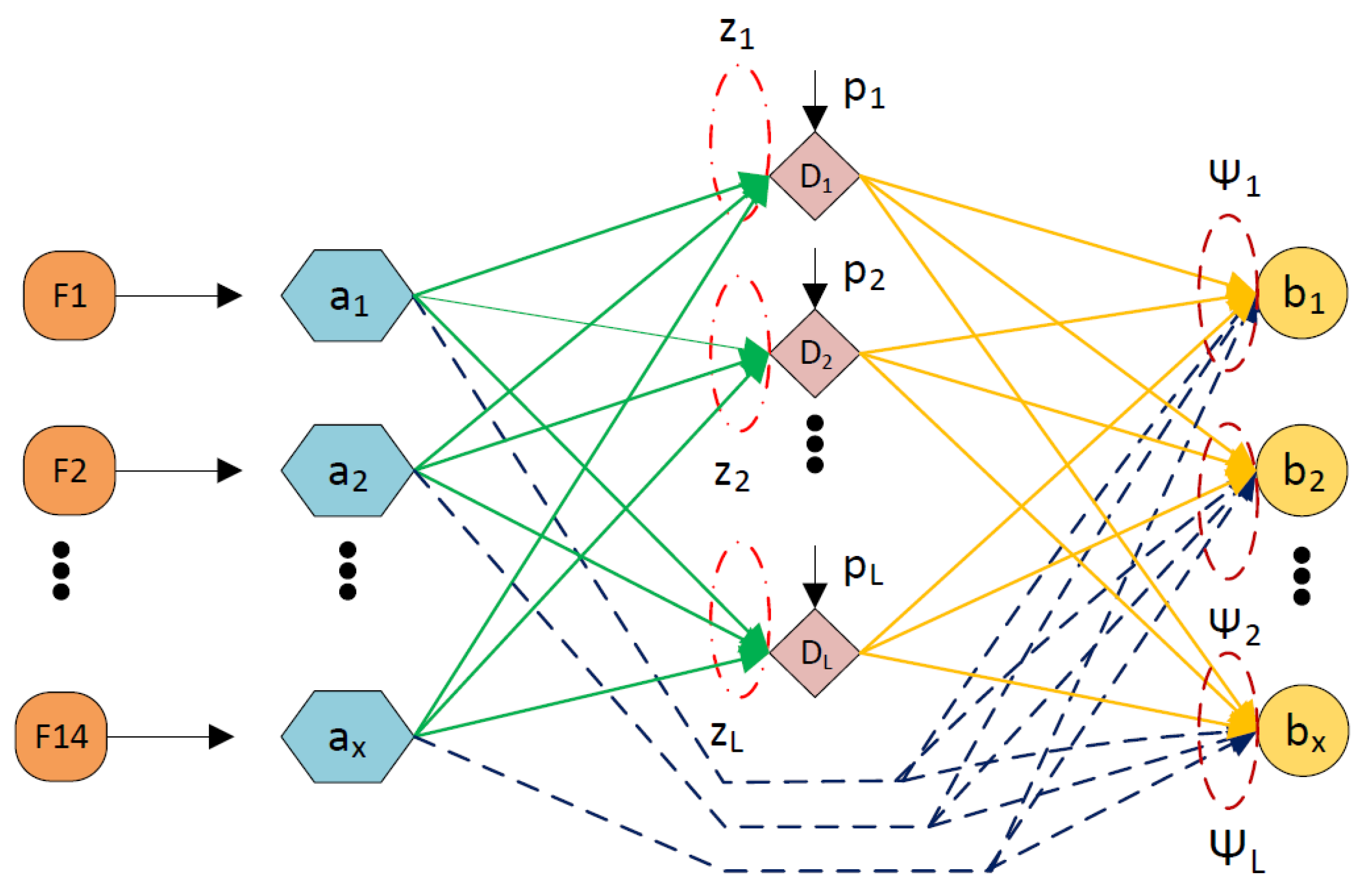
Figure 1. RVFLNs structure.
Energies 16 00252 g001
Figure 2. Flow chart of the Cauchy Distribution M-estimate RVFLNs.
Energies 16 00252 g002
Figure 3. IEEE 33-node distribution network.
Energies 16 00252 g003
Figure 4. The Fault Detection Accuracy of Different Methods.
Energies 16 00252 g004
Table 1. Feature Vectors for Fault Detection.
FeaturesNotationFormulation
F1In( φ i)tcurrent magnitude
F2Vn( φ i)tvoltage magnitude
F3 θ In( φ i)tcurrent angles
F4 θ Vn( φ i)tvoltage angles
F5d/dt(In)Derivative of Current magnitude
F6d/dt(Vn)Derivative of voltage magnitude
F7d/dt( θ In)Derivative of current angles
F8d/dt( θ Vn)Derivative of Voltage angles
F9 V n 1 j = 1 360 | S j |
F10 V n 2 j = 1 360 ( S j ) 2 1 / 2
F11 V n max | S j | j
F12 I n 1 j = 1 360 | S j |
F13 I n 2 j = 1 360 ( S j ) 2 1 / 2
F14 I n max | S j | j
Table 2. Fault dataset parameters.
Parameter TypeParameter ValueParameter Quantity
System Frequency/Hz 50 ± 5 % 1
System Voltage/kV121
Transition Resistance-ohm0, 30, 50, 1004
Table 3. Accuracy rates according to fault resistance values.
1P-G2PP-G2P-P3PPP
0 ohm100%100%100%100%
30 ohm100%100%100%100%
50 ohm100%96%95%98%
100 ohm100%94%93%97%
Table 4. Accuracy rates according to fault resistance values.
1P-G without Noise1P-G with Noise2P-G without Noise2P-G with Noise2P-P without Noise2P-P with Noise3PPP without Noise3PPP with Noise
0 ohm100%100%100%95%100%94%100%98%
30 ohm100%95%100%88%100%85%100%96%
50 ohm100%94%100%86%95%82%100%92%
100 ohm100%92%94%85%93%80%96%90%
Table 5. Comparison of train/test time.
Training Time (s)Testing Time (s)
Cauchy-M-RVFLN0.04700.0050
RVFLN0.002210.0050
CNN0.2470.576
LSTM0.6450.743
SVM0.8980.974
ELM0.4530.664
Table 6. Compared with Other Studies in the Literature.
TopologyData AcquisitionImplementationAlgorithmEffect of NoiseAccuracy (%)Disadvantages
[9]Single transmission line model3-phase currents inputMATLAB SimulinkSummation-Wavelet ELM, Summation-Gaussian ELMNoise was disregarded98.22Cannot train big data quickly and efficiently
[32](1) Three-phase double-ended system
(2) MMC-based back-to-back HVDC system
3-phase currents inputPSCAD softwareGroup sparse representationDifferent noise values were considered96.92Classification with limited memory and slows down significantly
[34]A five-bus power system3-phase currents input and square of currentsMATLAB simulation data were usedk-Nearest Neighbor algorithm (k-NN)Noise was disregarded98It is affected by noises
[37]33-node distribution network3-phase currents and voltages dataMATLAB simulation data were usedACNNNoise was disregarded95.80Large datasets take a long time to train
[41]Single transmission line model3-phase currents and voltages dataMATLAB simulation data were usedConvolutional sparse autoencoder (CSAE)Different noise values were considered92.22Important information may be lost
[43]Four-machine two-area test power system4 features input (current, current angle, voltage, voltage angle)MATLAB simulation data were usedLSTM method were usedNoise was disregarded96.71Easy overfitting, longer training times and sensitivity to random weight initialization
[68]Single transmission line model3-phase currents signals were usedMATLAB simulation data were usedSVM classifiersNoise was disregarded98.5It is affected by noises
[69]Single transmission line model3-phase current and voltage dataMATLAB simulation data were usedCNNNoise was disregarded99.99Large datasets take a long time to train
[70]Single transmission line model3-phase currents signals were usedMATLAB simulation data were usedk-means clusteringDifferent noise values were considered99.50It is affected by noises
Proposed method33-node distribution network14 different data inputRSCAD, RTDS simulatorCauchy-M-RVFLNDifferent noise values were considered89.94
Disclaimer/Publisher’s Note: The statements, opinions and data contained in all publications are solely those of the individual author(s) and contributor(s) and not of MDPI and/or the editor(s). MDPI and/or the editor(s) disclaim responsibility for any injury to people or property resulting from any ideas, methods, instructions or products referred to in the content.