Article

SMES-GCSC Coordination for Frequency and Voltage Regulation in a Multi-Area and Multi-Source Power System with Penetration of Electric Vehicles and Renewable Energy Sources

1
Electrical Engineering Department, Maulana Azad National Institute of Technology Bhopal, Bhopal 462003, India
2
Power Engineering Department, Faculty of Electrical Engineering, Computer Science and Information Technology, J. J. Strossmayer University of Osijek, K. Trpimira 2B, HR-31000 Osijek, Croatia
3
Department of Electrical and Electronics Engineering, National Institute of Technology Tiruchirappalli, Tiruchirappalli 620015, India
4
Electrical and Instrumentation Engineering Department, Thapar Institute of Engineering and Technology, Patiala 147004, India
*
Authors to whom correspondence should be addressed.
Energies 2023, 16(1), 251; https://doi.org/10.3390/en16010251
Submission received: 20 November 2022 / Revised: 21 December 2022 / Accepted: 22 December 2022 / Published: 26 December 2022

Abstract

:
Frequency, tie-line power, and the terminal voltages of synchronized generators must all be kept within prescribed limits to ensure the stability of an interconnected power grid through combined automatic generation control (AGC) and automatic voltage regulator (AVR) loops. Thermal power plants, electric vehicles, and renewable energy sources—including solar and wind, geothermal, and solar thermal power plants—form the two-area integrated power system in present research. A new cascade controller named the cascaded proportional integral derivative (PID) and fractional-order PID (CPID-FOPID) controller is proposed for the first time, whose performance is compared with the PID and FOPID controller. The results show that the proposed cascade controller outperforms PID and FOPID in delivering superior dynamic characteristics, including short settling times and low oscillation amplitudes. A new metaheuristic algorithm named the coot algorithm was applied to optimize the parameters of these controllers. The suggested controller outperforms FOPID in the combined AGC and AVR problem under uncertain conditions (random load disturbance, variable input of solar irradiation, and wind power). Robustness of the controller is tested with significant variation in the turbine time constant of the thermal and geothermal power plant. In this study, authors also investigated the best possible coordination between the superconducting magnetic energy storage (SMES) and gate-controlled series capacitor (GCSC) devices to control both voltage and frequency simultaneously. The effect of communication time to the power system is analyzed in this study. Additionally, the obtained results are satisfactorily validated using OPAL-RT real-time digital simulator.

1. Introduction

In an integrated power system having several control zones, power system engineers are primarily concerned with maintaining frequency and voltage levels close to optimal operating conditions. By balancing load demand with generation and related losses, a well-maintained power system is supposed to provide uninterrupted, high-quality power to its customers. In a real-time situation, the load changes continuously, so there exist fluctuations in frequency and voltage. To keep these variations within acceptable limits, each generator needs two control loops: an automatic generation control (AGC) and an automatic voltage regulator (AVR) [1,2].
Frequency and voltage oscillations may become more pronounced and even cause system instability due to the lack of inertia in photovoltaic (PV) systems. Due to the depletion of traditional energy sources, rising fuel costs, and environmental warming conditions, incorporating renewable energy sources (RES) is increasing in the current fossil fuel-based power system. As a substitute to traditional fossil fuels, RES, such as wind power generation (WPG) and solar photovoltaic (SPV) generation, have captured the interest of researchers [1,3,4,5].
The controlling of the renewable energy sources is challenging since they strongly depend on climate factors. To overcome this issue, storage devices, such as SMES, flywheels, and batteries, can be used in combination with RES to improve grid stability and frequency fluctuations [2,5]. At times of high demand from the grid, these devices release their stored energy. At the same time, non-petroleum-dependent alternatives such as electric vehicles (EVs) are growing in favor as eco-friendly alternatives to traditional gasoline automobiles that can contribute to a greener future.
These EVs have the potential to serve as energy storage devices that aid in frequency regulation as a source during the times of high demand [1]. To address the AGC issue, a few research studies have been conducted on EV penetration [6,7,8,9,10]. Authors in [6,7] analyzed the effect of EV and communication delay on isolated power systems. Utilizing EV for AGC accentuates the reorganized power market [8]. However, research on EV integration for combined AGC and AVR is in its infancy and requires attention [11].
The superconducting magnetic energy storage (SMES) technology can manage both real and reactive power requirements. The SMES system functions as energy-compensating equipment for larger loads and therefore controls frequency oscillations [2,12]. The SMES action is faster than the primary control mechanism of the governor [12]. Frequently charging and discharging of a battery system to handle power system fluctuations reduces its lifespan and performance. The SMES technology is preferable over battery systems [12,13,14]. However, the superiority of the SMES system in managing the active and reactive powers together having solar PV, wind, geothermal, and thermal power plants is yet to be determined in the presence of a cascaded controller.
Flexible AC transmission system (FACTS) devices enhance the power system’s transfer capacity and stability. Series FACTS devices, such as the thyristor-controlled series capacitor (TCSC), the static synchronous series compensator (SSSC), the thyristor-controlled phase shifter (TCPS), the interline power flow controller (IPFC), and the gate-controlled series capacitor (GCSC), demonstrate their efficacy in managing the tie-line powers in AGC [15,16]. Among all FACTS devices, the GCSC has recently captured the attention researchers in AGC studies due to its numerous benefits [16]. The GCSC has a smaller capacitor size, lower cost, and stronger compensating capabilities than the TCSC. The GCSC is simpler and more cost-effective than the TCPS and SSSC [17,18]. References [13,14] have studied the coordination of SMES-TCSC and SMES-SSSC; however, the coordination of SMES with GCSC is not found in the literature addressing combined AGC and AVR loop problems.
In order to regulate the frequency and voltage fluctuations in AGC and AVR loops, suitable controllers are required. Various integer order controllers [2,3,19] and proportional integral derivative (PID) controllers [1,2,11,20,21,22] have been used in the past to solve AGC and AVR difficulties in literature. Because of its low price, ease of use, and reliability in practice, the PID controller is mostly used in the literature. However, it fails when applied to systems with non-minimum phase [1,11,23,24]. Later, the fractional order PID (FOPID) controllers were successfully implemented to address the AGC and/or AVR [25,26] and demonstrated their superiority over integer order controllers because of their extra knobs for flexible control action. Recently, studies have focused on the cascade control arrangement (CCA) in relation to AGC and/or AVR difficulties [19]. The CCA adds a sensor that helps in reducing the disturbance before it affects the output of the plant.
To improve the performance of a controller, its parameters must be optimally optimized using appropriate metaheuristic algorithms. Shukla et al. [1] used the particle swarm optimization (PSO) algorithm to obtain gains of PID and TID controllers. The authors of [2,20] used a hybrid algorithm of artificial electric field to get the variables of PID controller. The authors of [3] applied gradient-based optimization (GBO) to optimized integral order controllers. Ramoji and Saikia in [11,23,24] utilized Harris hawks optimization (HHO) in their work. The PSO technique has a tendency to fall into a local optimum in a larger dimensional search space with slow convergence nature [27]. The HHO suffers from the drawbacks such as population diversity and local optima [28].
Inspired by the actions of birds with the same name, a new metaheuristic algorithm called the coot algorithm (CA) was presented recently by Naruei and Keynia [29]. In addition to tackling real-world optimization issues like the design of a pressure spring tension, their analysis demonstrates that the CA outperforms most other optimization methods, suggesting that it be investigated further when creating a controller for the combined AGC and AVR issue. The CA successfully applied to address the unimodal and multimodal test functions. The CA proved its efficiency in solving the problems that have unknown search spaces.
The field of AGC and AVR investigations has the following limitations, according to a careful examination of the literature.
  • The AGC and AVR loops control with the utilization of cascaded PID-FOPID controllers tuned by coot technique has not yet been observed.
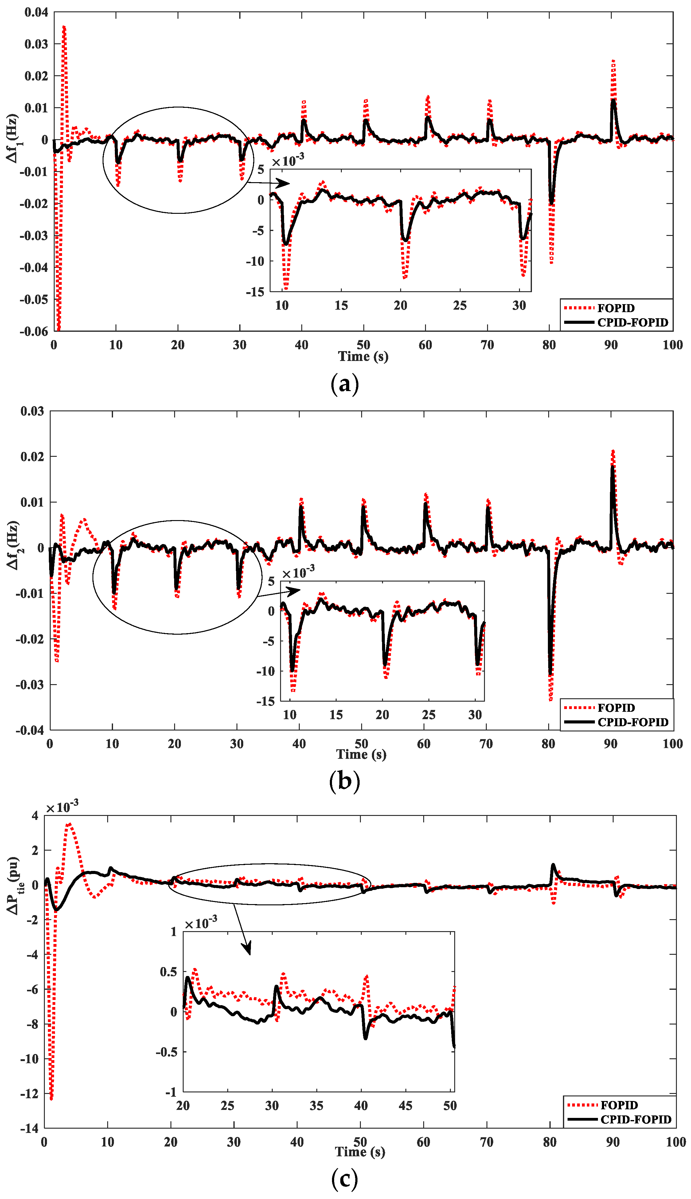
  • The investigations showing the comparative behaviors of cascaded PID-FOPID, FOPID, and PID controllers is not found for the system comprising renewable energy sources and electric vehicles.
  • The coordinated performance of GCSC and SMES in regulating frequency and voltage with the cascade PID-FOPID controller is not known.
  • Further research is needed on the time-delay effect on the combined AGC and AVR system performance in the presence of a coot-based cascaded PID-FOPID.
The above limitations encourage the authors to investigate them in the present research for combined AGC and AVR issue. Based on the limitations found in the literature review, the following are the novel contributions of this research:
  • To examine the comparative performance of cascaded PID-FOPID controllers with PID and FOPID controllers to evaluate the superiority of the proposed controller when optimized with the coot technique.
  • To demonstrate the efficiency of a cascaded PID-FOPID controller over FOPID random disturbances and variable solar and wind input.
  • To examine the optimal configuration for the application of GCSC and SMES coordination to the combined AGC and AVR problem by comparing SMES-SMES, GCSC, and SMES-GCSC-SMES coordination strategies.
  • To investigate the impact of communication delay on frequency and voltage profile in the presence of a cascaded PID-FOPID controller and to suggest a suitable delay margin for the considered interconnected system.
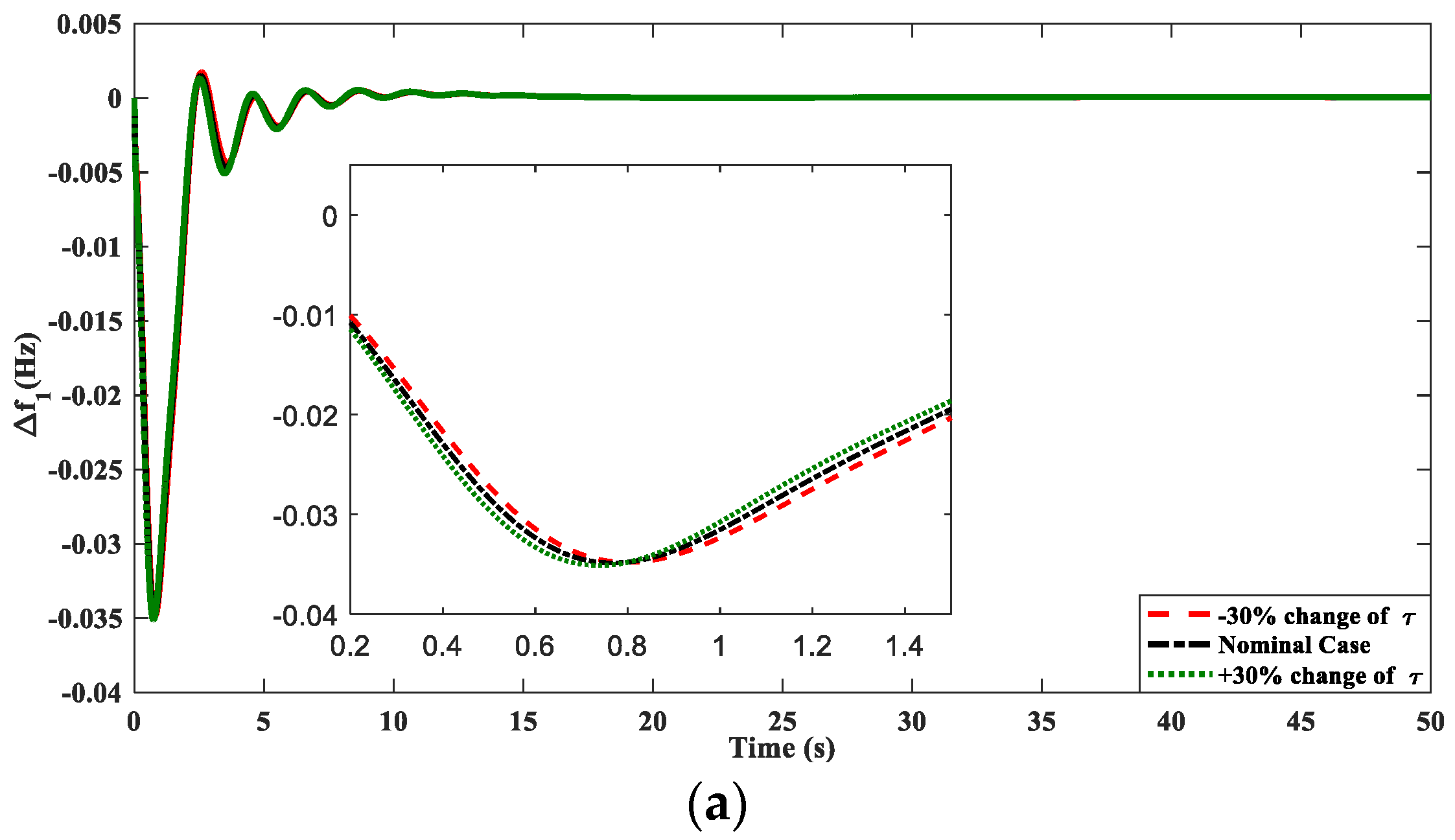
  • To validate the stability of CA-based cascaded PID-FOPID controllers against fluctuations in turbine time constants of thermal and geothermal power plants.
  • To validate simulation findings using an OPAL-RT 4510 real-time digital simulator.
For the benefit of the reader, a schematic overview of different sources utilized is presented in Figure 1, namely, the reheat thermal power plant (RTPP), geothermal power plant (GTPP), solar thermal power plant (STPP), solar photovoltaic (SPV), and wind turbine generation (WTG) along with electric vehicles. The control system represented in the figure acts as control center. The power and communication networks are also highlighted. Various kinds of power system elements, such as loads and SMES, are also depicted. Table 1 highlights the comparative analysis of previously published articles, including the current manuscript.
The individual segments of this work are structured as follows. Section 2 describes the power systems under investigation. Section 3 discusses the proposed CPID-FOPID controller structure used for frequency and voltage regulation. The coot technique is explained in Section 4. Section 5 discusses the findings for all test systems, along with OPAL-RT validation of the collected results. Finally, the conclusions and recommendations for further study are offered in Section 6.

2. System Investigated

An interconnected two-area power system is taken for investigation having equal sources in both the areas. Small signal analysis is done in this study; thus, the power system’s transfer function-based model is represented in Figure 2a,b. The considered system has the following sources in each area: a reheat thermal power plant (RTPP) [1,2], a geothermal power plant (GTPP) [19], and a solar thermal power plant (STPP) [24]. From the renewable energy source (RES), solar photovoltaic (SPV) [1] and wind turbine generation (WTG) [1] are connected in both the areas along with electric vehicles (EVs) [8,9]. All the gain and time constants of the above discussed sources are mentioned in the Appendix A. The system under study is considered an equal area capacity ratio, i.e., 10,000 MW in each area. To make the realistic approach, the system is also incorporated with non-linearities of the reheat turbine, GRC (Figure 2c), and communication time delay. The authors also study the combined coordination effect of FACTS (GCSC) and storage devices (SMES).
The application of electric vehicles (EVs) is considered in vehicle to gride (V2G) mode. The EVs are comparable to energy storage devices, such as batteries, that may contribute to frequency control [8,9,10]. A single electric vehicle can produce up to 20 kW [8,9]. Therefore, an EV aggregator is required for AGC and AVR problems that typically include MW-range capacities. EVs often include a dynamic model of an EV aggregator, a time delay, a dead band, and regulating capacity [8,9] (Figure 2d). The maximum and minimum output powers of the EV aggregator are denoted as Δ P E V a U and Δ P E V a U , which are related to incremental generation change (∆PEV) in any area, as shown in Equation (1).
Δ P E V a U = Δ P E V N E V Δ P E V a D = Δ P E V N E V
where NEV is the total number of electric vehicles connected to the grid. This study assumed that each EV has the ∆PEV of 5 kW, and there are 8000 numbers of such EVs connected in each area.

3. Controller Structure

To find out the solution of the two-area combined AGC and AVR issue, a cascaded controller is utilized. The primary purpose of the cascaded controller is to improve the disturbance rejection for multi-loop issues like frequency regulation [19]. The two controllers in this setup, designated as C1(s) and C2(s), are referred to as the master (M) and slave (S) controllers, respectively. The control mechanism for the cascade is depicted in Figure 3a, along with C1(s) and C2(s).
Area control error (ACE) refers to the error reported to the controller. When system loading changes, frequency, and tie-line powers diverge from their nominal or scheduled values, it is undesirable and can lead to power system failure. Continuous monitoring between load demand and generation in AGC reduces ACE. The ACE is a linear combination of frequency and tie-line power variations (Equations (2) and (3)).
A C E 1 = β 1 Δ f 1 + Δ P t i e
A C E 2 = β 2 Δ f 2 + a 12 Δ P t i e
The β1 and β2 are frequency response characteristics, which are the same as the frequency bias constant (Bi); Δf1 and Δf2 are the deviation in area frequency; ΔPtie and a12 are deviation in tie-line power flow and area rating ratio, respectively.
The fractional order is governed by the generalized integer order calculus. This presents the most frequently used integrators and Reimann–Liouville (RL) fractional derivatives in Equations (4) and (5).
D t α a f t = 1 Γ q α d q d t q a t t τ α 1 + q f τ d τ ,   q 1 α q
D t α a f t = 1 Γ α a t t τ α 1 f τ d τ
The terms a, t, D t α , and Γ q α denote initial time instance, final time instance, differential fractional operator, and Euler’s gamma function, respectively. The “q” takes the integer values whose rage is q − 1 ≤ αq.
Specifically, the transfer functions of a cascade combination of PID-FOPID controller is shown in Figure 3b.
C 1 s = G s P I D w = K P w + K I w s + K D w s
C 2 s = G s F O P I D w = K P w + K I w s λ + K D w s μ
The terms G s P I D w and G s F O P I D w are the master and slave controllers, respectively, with their derivative, integral, and proportional gains representing K D w , K I w , and K P w in area w and corresponding integral and derivative powers of λ and µ, respectively.
Finding a solution within the feasible zone is the goal of optimization problems, which are solved by limiting some objective function chosen for the system. The integral time absolute error (ITAE) criterion, as shown in Equation (8), is used as the objective function for the combined AGC and AVR problem under investigation.
J I T A E M I N = 0 T Δ f 1 + Δ f 2 + Δ P t i e + Δ V 1 + Δ V 2 t . d t
where Δfw, ΔVw, and ΔPtie are the fluctuations in frequency, voltage, and transmission lines, respectively. The terms t and T denote time instance and simulation durations, respectively.

4. Coot Algorithm

The coot algorithm (CA) was recently proposed by Nauei and Keynia [29]. It is inspired by the behavior of coots as they seek food on the water’s surface. This technique is modelled after the two phases of motion done by coot birds to guide their swarm towards a predetermined destination. In CA, the random population X i = x 1 , x 2 , x 3 , x n serves as the baseline for continuous evaluation against the objective function. Based on four types of motion, the algorithm is formulated below.

4.1. Random Motion

The random motion of the coot at different position CP(i) is given by Equation (9)
C P ( i ) = C P ( i ) + A R 2 ( Q C P ( i ) )
where R2 is random number [0, 1], and A is described by Equation (10) in terms of maximum iterations (maxitr).
A = 1 i t r max   i t r

4.2. Chain Movement

This movement is implemented by Equation (11) by taking the average position of the two coots CP(i) and CP(i − 1).
C P ( i ) = 0.5 ( C P ( i 1 ) + C P ( i ) )

4.3. Position Adjustment as Per Group Leader

The selection of leader for execution of this position is calculated by Equation (12).
K = 1 + ( i M O D   N L )
where NL is the total number of leaders and K is the leader index. The next updated position of the coot based on the leader is represented as Equation (13)
C P ( i ) = L P ( k ) + 2 R 1 cos ( 2 π R ) L P ( k ) C P ( i )
where LP is the position of the leader, and R1 and R are the random numbers between the range of [0, 1] and [−1, 1], respectively.

4.4. Leader Movement

To get the optimal place, the group leader must keep its position update as per Equation (14).
L P ( i ) = B R 3 cos ( 2 π R ) ( g B e s t L P ( i ) + g B e s t ) + g B e s t R 4 < 0.5 L P ( i ) = B R 3 cos ( 2 π R ) ( g B e s t L P ( i ) + g B e s t ) - g B e s t R 4 0.5
where gBest is the overall best solution, and R3 and R4 are random numbers in the range [0, 1]. The B is found using Equation (15).
B = 2 i t r max   i t r
For this study, the number of search agents (n) is set to 10, and the number of iterations (max itr) is taken to 100 to optimize all the controller parameter subjected to Equation (8).

5. Results Analysis

This research work is conducted on a Windows 10Pro PC running with MATLAB/SIMULINK 2016a, with an Intel core i7-8700 CPU, 3.2 GHz clock speed, and 8 GB RAM. Improved results for the cascade controller are emphasized in bold.

5.1. At Nominal Conditions

This study evaluates the combined AGC and AVR for two equal 1000 MW power systems, as depicted in Figure 1a. In this case, 2% step load perturbated (SLP) disturbance is used in both areas (i.e., ∆PD1 = ∆PD2 = 1000 MW 0.02 = 20 MW at t = 0 s). In both areas, the geothermal power plant (GTPP), reheat thermal power plant (RTPP) with GRC, wind turbine generator, photovoltaic system, and electric vehicle (EV) are considered for power generation. Different secondary controllers, namely proportional integral derivative (PID), fractional order PID (FOPID), and cascaded PID-FOPID, are utilized to examine the system. To get the parameters of these controllers, the coot algorithm (CA) is used, and the results are subjected to Equation (8).
The Js (ITAE) value for the PID controller is 3.42, while it is 2.155 for the FOPID controller and 1.156 for the cascaded PID-FOPID controller. This shows that the cascaded controller is better than the PID and FOPID controllers in respect to Js.
The coot algorithm is executed for each controller in order to obtain its parameters. The parameters of the controller (PID, FOPID, and cascaded PID-FOPID) obtained by the CA are shown in Table 2, Table 3 and Table 4. Figure 4 illustrates the system dynamics for frequency variation in area 1 and 2 (i.e., ∆f1 and ∆f1), change in tie line power (∆Ptie), and pu terminal voltage for AVR 1 and 2 (i.e., Vt1 and Vt2).
Evaluation of Figure 4 is shown in Table 5 and Table 6, with comparisons made between peak overshoot (MP), peak undershoot (UP), and settling time (Ts). The following is a critical analysis of the cascaded controller, based on Table 5: The MP values for ∆f1, ∆f2, and ∆Ptie are 0.00148 Hz, 0.001068 Hz, and 0.00381 puMW, respectively. The UP values are 0.03485 Hz, 0.0432 Hz, and 0.00177 puMW, and the Ts values are 13.55 s, 12.16 s, and 24.11 s, respectively.
The cascaded controller for AVR1 (Table 6) provides an MP value of 1.02 pu, which is 39.29% better than PID and 14.35% better than FOPID, while the cascaded controller for AVR2 yields an MP value of 1.063 pu, which is 35.18% better than PID and 32.72% better than FOPID. The settling times (Ts) for the cascaded controller, PID, and FOPID are 14.2 s, 16.33 s, and 38.98 s for AVR 1, and 11.87 s, 15.26 s, and 20.98 s for AVR 2, repectively. Therefore, the cascaded PID-FOPID is superior to PID and FOPID in terms of MP, UP, and Ts for the combined AGC and AVR problem.

5.2. Effect of Random Load Demand (RLD), Variable Solar Irradiations, and Irregular Wind Power

The studies done so far have assumed constant solar irradiances and wind power, as well as a 2% step disturbance. However, under realistic conditions, these vary continuously. To evaluate this circumstance, the random load demand (RLD), variable solar irradiations, and irregular wind power depicted in Figure 5 are considered. The performance of the proposed cascade controller is compared to that of the FOPID controller after parameters are obtained via the coot algorithm (Table 7 and Table 8). When using the proposed coot-based cascade controller, the overshoots (MP) and undershoots (US) are reduced to a greater extent than they are with the FOPID controller. This is an indication of the superiority of the cascade controller. The dynamics (i.e., ∆f1, ∆f2, ∆Ptie, Vt1, and Vt2) are depicted in Figure 6.

5.3. Sensitivity Analysis

It is anticipated that the operating circumstances of the power system will vary continuously, and the controller gains must be capable of adapting the system performance for these fluctuations. The sensitivity analysis is performed to validate the capacity of the controller’s nominal parameters to perform their function. In this scenario, the time constants of the turbines of RTPP and GTPP are modified by ±30% of both areas. The system dynamics (i.e., ∆f1, ∆f2, ∆Ptie, Vt1, and Vt2) are compared for with and without varied conditions in Figure 7. It can be observed from this comparison that the responses are nearly same, which demonstrates the robustness of the cascade controller with same parameters obtained at nominal conditions.

5.4. SMES-GCSE-SMES Coordination

The superconducting magnetic energy storage (SMES) technology stores electrical power from the grid as the magnetic field of a coil composed of superconducting wire with almost negligible energy loss. Although secondary control actions are slow to respond, the SMES system can improve the system’s dynamic behavior and power flow [12,13,14].
The SMES system incorporates a step-down transformer, as well as an AC/DC converter, a superconducting inductor, and a converter unit. Figure 8 illustrates the schematic diagram of the SMES.
Figure 9 is a representation of its corresponding transfer function model. In this figure, KSMES and TSMES stand for the gains and time constants, respectively. The lead-lag compensation block parameters are expressed by the terms T1, T2, T3, and T4, respectively. The SMES units are placed at the load points of areas 1 and 2. Notations in the SMES, such as KSMES, TSMES, T1, T2, T3, and T4, are tuned along with the parameters of the cascaded controller for the purpose of achieving its best possible design. Equation (16) describes the transfer function of the SMES system.
T F S M E S = Δ P S M E S Δ f 1 + s T 1 1 + s T 2 1 + s T 3 1 + s T 4 K S M E S 1 + s T S M E S
The gate-controlled series capacitor (GCSC), which is a series FACTS device based on a pair of gate-commutated switches in parallel with a capacitor, can control the power flow of the transmission lines and its impedance. The schematic diagram is shown in Figure 10.
This article represents different coordination of the above discussed SMES and GCSC. The purpose of this section is to find the best coordination from SMES-SMES, GCSC, and SMES-GCSC-SMES. Table 9 represents gain obtained by the cascaded controller when optimized with CA for SMES-SMES coordination, and Table 10 indicates the optimized values of SMES for this case. Table 11 represents gain obtained by the cascaded controller when optimized with CA for GCSC coordination. Table 12 and Table 13 represent gain obtained by the cascaded controller when optimized with CA for SMES-GCSC-SMES coordination and optimized SMES parameters for this case, respectively.
Figure 11 represents the comparison of system dynamics (i.e., ∆f1, ∆f2, ∆Ptie, Vt1, and Vt2) with the different coordination scheme with nominal case. Among these, coordination SMES-GCSC-SMES found the best results, which is also proven by Table 14 and Table 15, with comparisons made between OP, UP, and Ts.

5.5. Effect of Communication Time Delay

It is believed that the control signal travels with a certain delay from the distant location to the control center. As a result of these delays, the dynamic behaviors degrade. For this study, the controller receives a single delay signal representing the whole communication delay. Different communication time delays (Td) are placed on the system, and the dynamics (i.e., ∆f1, ∆f2, ∆Ptie, Vt1, and Vt2) of the system (shown in Figure 12) are studied to see how well the controller works. As shown in Figure 12, as the Td value rises, the system dynamics are affected by an increase in oscillations.
Up to Td = 1.6 s, the system dynamics are well-settled, but after applying a delay longer than 1.6 s, the dynamics degrade in nature, and at Td = 1.85 s, the fluctuations increase and oscillate continuously. The system dynamics become more oscillatory as Td increases, which is 1.85 s or more. Therefore, for the proposed system to operate reliably, a delay of less than 1.85 s is recommended. The optimized gain of the cascaded controllers obtained at delay of 1.6 s and 1.85 s are mentioned in Table 16 and Table 17, respectively.

5.6. Validaton of the Dynamics through OPAL-RT

The proposed automatic voltage regulator (AVR) and automatic generator controller (AGC) system for two-area power plants is verified on the OPAL-RT OP4510 real-time digital simulator, which makes use of the most up-to-date Intel generation Xeon 4-core processors and a robust Xilinx Kintex-7 FPGA platform. It is capable of real-time parallel processing, producing results that are matched with those obtained on hardware [23,24]. Figure 13 depicts the OPAL-RT OP4510 system in its laboratory configuration, which includes a host PC running RT-Lab software, I/O ports, TCP/IP connection, and the real-time digital simulator itself. In order to validate the proposed unified ALFC and AVR control pattern, it is first constructed in the MATLAB/Simulink R2018 platform. The technique combines the parallel processing power of the real-time simulator. The results from the system are compared to the results from using MATLAB. In-depth analysis of the results (Figure 14) shows that the system outputs (i.e., ∆f1, ∆f2, ∆Ptie, Vt1, and Vt2) on both platforms are quite equivalent, lending support to the validity of the suggested method.

6. Conclusions

In this paper, the suppression of oscillations in the dynamics of the combined AGC and AVR system are performed utilizing a coot algorithm-tuned CPID-FOPID controller on the study considering two equal-area power systems with the following sources: reheat thermal power plant (RTPP) in addition to GRC, geothermal power plant (GTPP), solar thermal power plant (STPP), solar photovoltaic (SPV), and wind turbine generation (WTG). In this study, the power system was penetrated with electric vehicles (EVs) in both areas that serve as sources for the grid (V2G mode). The main findings of this research are explained below.
  • The analysis revealed that the proposed cascaded controller is superior to the PID and FOPID controllers in terms of peak overshoot (MP), peak undershoot (UP), and settling time (Ts) when optimized using the coot algorithm.
  • To verify the stability of the controller, the power system is also examined with realistic approaches, such as random load demand (RLD), fluctuating solar irradiances, and irregular wind powers. Even under these more real circumstances, the cascaded controller is superior to the FOPID controller.
  • For the purpose of verifying the proposed controller’s efficacy, a sensitivity analysis is conducted in which the RTPP and GTPP turbine time constants are varied by +/-30%. This case study successfully confirms the CPID-FOPID controller capacity to survive these fluctuations, as the dynamics obtained under these conditions were found to be identical to those in the nominal case.
  • The SMES-GCSC-SMES coordination is successfully verified with the CPID-FOPID controller.
  • Moving toward a more realistic scenario, this article also addressed the impact of communication time delay, which degrades the system’s dynamics when introduced into the system.
  • The obtained simulation findings are successfully verified with validation using OPAL-RT OP4510 real-time digital simulator.
However, the research presented in this manuscript is limited to conventional power system, and the restructured AGC or combined AGC-AVR problem can be evaluated using the proposed coot algorithm-tuned cascaded controller. As the fuzzy logic controller provides superior performance, the combination of cascaded fuzzy-based controllers can be tested for the frequency and voltage regulation in an interconnected power system. As the number of tunable parameters are more in the fractional or cascaded controller, proper care should be taken when optimizing these controllers. The above-mentioned controllers can be designed utilizing the more efficient optimization technique, which delivers competitive global optimum results.

Author Contributions

Conceptualization, H.S. and M.R.; data curation, S.N., P.K. and A.S.R.; formal analysis, M.R. and P.K.; funding acquisition, H.S. and M.R.; methodology, H.S., M.R., P.K. and A.S.R.; project administration, S.N. and A.S.R.; resources, H.S. and M.R.; software, P.K. and S.N.; supervision, P.K. and S.N.; validation, H.S. and M.R.; visualization, A.S.R. and P.K.; writing—original draft, H.S. and M.R.; writing—review and editing, P.K., S.N. and A.S.R. All authors have read and agreed to the published version of the manuscript.

Funding

This research received no external funding.

Institutional Review Board Statement

Not applicable.

Informed Consent Statement

Not applicable.

Data Availability Statement

None.

Conflicts of Interest

The authors declare no conflict of interest.

Appendix A

Reheat Thermal Power Plant:
Governor time constant (Tg) = 0.08 s,
Turbine time constant (Tt) = 0.3 s,
Reheater gain (Kr) = 0.5,
Reheater time constant (Trt) = 10 s.
Geothermal Power Plant:
Governor time constant (Tg) = 0.05 s,
Turbine time constant (Tt) = 0.1 s.
Solar Thermal Power plant:
Solar collector gain (Ksi) = 1,
Solar collector time constant (Tsi) = 1,
Governor time constant (Tsg) = 0.08 s,
Turbine time constant (Tst) = 3 s.
Power System:
Power system gain (KP) = 120,
Power system time constant (TP) = 20 s,
Synchronizing coefficient (T12) = 0.0707 puMW/rad.
Electric Vehicle:
Gain (KEV) = 1,
Time constant (TEV) = 1 s.
Solar Photovoltaic:
Gain (KPV) = 1,
Time constant (TPV) = 1.8 s.
Wind Turbine Generator:
Gain (KWTG) = 1,
Time constant (TWTG) = 1.5 s
Automatic Voltage Regulator:
Amplifier gain (Ka) = 10,
Amplifier time constant (Ta) = 0.1 s,
Exciter gain (Ke) = 1,
Exciter time constant (Te) = 0.4 s,
Generator field circuit gain (Kf) = 0.8,
Generator field circuit time constant (Tf) = 1.4,
Sensor gain (Ks) = 1,
Sensor time constant (Ts) = 0.05 s,
Cross-coupling coefficients of AVR: K1 =1, K2 = 0.1, K3 = 0.5, K4 = 1.4, and PS = 0.145.
GCSC:
Gain (KGCSC) = 1,
Time constant (TGCSC) = 0.015 s
Controller:
KDw, KIw, and KPw denote the derivative, integral, and proportional gains in area w, respectively.
λ and µ represent the powers of integral and proportional gains, respectively.

References

  1. Shukla, H.; Nikolovski, S.; Raju, M.; Rana, A.S.; Kumar, P. A Particle Swarm Optimization Technique Tuned TID Controller for Frequency and Voltage Regulation with Penetration of Electric Vehicles and Distributed Generations. Energies 2022, 15, 8225. [Google Scholar] [CrossRef]
  2. Kalyan, C.N.S.; Goud, B.S.; Reddy, C.R.; Bajaj, M.; Sharma, N.K.; Alhelou, H.H.; Siano, P.; Kamel, S. Comparative Performance Assessment of Different Energy Storage Devices in Combined LFC and AVR Analysis of Multi-Area Power System. Energies 2022, 15, 629. [Google Scholar] [CrossRef]
  3. Hossam-Eldin, A.A.; Negm, E.; Ragab, M.; AboRas, K.M. A Maiden Robust FPIDD2 Regulator for Frequency-Voltage Enhancement in a Hybrid Interconnected Power System Using Gradient-Based Optimizer. Alex. Eng. J. 2022, in press. [Google Scholar] [CrossRef]
  4. Kumar, V.; Sharma, V.; Naresh, R. Leader Harris Hawks Algorithm Based Optimal Controller for Automatic Generation Control in PV-Hydro-Wind Integrated Power Network. Electr. Power Syst. Res. 2023, 214, 108924. [Google Scholar] [CrossRef]
  5. Singh, B.; Slowik, A.; Bishnoi, S.K. A Dual-Stage Controller for Frequency Regulation in a Two-Area Realistic Diverse Hybrid Power System Using Bull–Lion Optimization. Energies 2022, 15, 8063. [Google Scholar] [CrossRef]
  6. Naveed, A.; Sonmez, S.; Ayasun, S. Impact of Electric Vehicle Aggregator with Communication Time Delay on Stability Regions and Stability Delay Margins in Load Frequency Control System. J. Mod. Power Syst. Clean Energy 2021, 9, 595–601. [Google Scholar] [CrossRef]
  7. Tripathi, S.; Singh, V.P.; Kishor, N.; Pandey, A.S. Load Frequency Control of Power System Considering Electric Vehicles’ Aggregator with Communication Delay. Int. J. Electr. Power Energy Syst. 2023, 145, 108697. [Google Scholar] [CrossRef]
  8. Khan, M.; Sun, H. Complete Provision of MPC-Based LFC By Electric Vehicles with Inertial and Droop Support from DFIG-Based Wind Farm. IEEE Trans. Power Deliv. 2022, 37, 716–726. [Google Scholar] [CrossRef]
  9. Khan, M.; Sun, H.; Xiang, Y.; Shi, D. Electric Vehicles Participation in Load Frequency Control Based on Mixed H2/H∞. Int. J. Electr. Power Energy Syst. 2021, 125, 106420. [Google Scholar] [CrossRef]
  10. Debbarma, S.; Dutta, A. Utilizing Electric Vehicles for LFC in Restructured Power Systems Using Fractional Order Controller. IEEE Trans. Smart Grid 2017, 8, 2554–2564. [Google Scholar] [CrossRef]
  11. Ramoji, S.K.; Saikia, L.C. Utilization of Electric Vehicles in Combined Voltage-frequency Control of Multi-area Thermal- Combined Cycle Gas Turbine System Using Two Degree of Freedom Tilt-integral-derivative Controller. Energy Storage 2021, 3, 1–20. [Google Scholar] [CrossRef]
  12. Morsali, J. Fractional Order Control Strategy for Superconducting Magnetic Energy Storage to Take Part Effectually in Automatic Generation Control Issue of a Realistic Restructured Power System. J. Energy Storage 2022, 55, 105764. [Google Scholar] [CrossRef]
  13. Nandi, M.; Shiva, C.K.; Mukherjee, V. Frequency Stabilization of Multi-Area Multi-Source Interconnected Power System Using TCSC and SMES Mechanism. J. Energy Storage 2017, 14, 348–362. [Google Scholar] [CrossRef]
  14. Bhatt, P.; Roy, R.; Ghoshal, S.P. Comparative Performance Evaluation of SMES-SMES, TCPS-SMES and SSSC-SMES Controllers in Automatic Generation Control for a Two-Area Hydro-Hydro System. Int. J. Electr. Power Energy Syst. 2011, 33, 1585–1597. [Google Scholar] [CrossRef]
  15. Pilla, R.; Azar, A.T.; Gorripotu, T.S. Impact of Flexible AC Transmission System Devices on Automatic Generation Control with a Metaheuristic Based Fuzzy PID Controller. Energies 2019, 12, 4193. [Google Scholar] [CrossRef] [Green Version]
  16. Raju, M.; Saikia, L.C.; Sinha, N. Load Frequency Control of a Multi-Area System Incorporating Distributed Generation Resources, Gate Controlled Series Capacitor along with High-Voltage Direct Current Link Using Hybrid ALO-Pattern Search Optimised Fractional Order Controller. IET Renew. Power Gener. 2019, 13, 330–341. [Google Scholar] [CrossRef]
  17. Oshnoei, S.; Oshnoei, A.; Mosallanejad, A.; Haghjoo, F. Contribution of GCSC to Regulate the Frequency in Multi-Area Power Systems Considering Time Delays: A New Control Outline Based on Fractional Order Controllers. Int. J. Electr. Power Energy Syst. 2020, 123, 106197. [Google Scholar] [CrossRef]
  18. Oshnoei, A.; Kheradmandi, M.; Khezri, R.; Mahmoudi, A. Robust Model Predictive Control of Gate-Controlled Series Capacitor for LFC of Power Systems. IEEE Trans. Industr. Inform. 2021, 17, 4766–4776. [Google Scholar] [CrossRef]
  19. Dekaraja, B.; Saikia, L.C. Combined Voltage and Frequency Control of Multiarea Multisource System Using CPDN-PIDN Controller. IETE J. Res. 2021, 1–16. [Google Scholar] [CrossRef]
  20. Kalyan, C.H.N.S.; Rao, G.S. Impact of Communication Time Delays on Combined LFC and AVR of a Multi-Area Hybrid System with IPFC-RFBs Coordinated Control Strategy. Prot. Control. Mod. Power Syst. 2021, 6, 1–20. [Google Scholar] [CrossRef]
  21. Sahoo, S.C.; Barik, A.K.; Das, D.C. Synchronized Voltage-Frequency Regulation in Sustainable Microgrid Using Novel Green Leaf-Hopper Flame Optimization. Sustain. Energy Technol. Assess. 2022, 52, 102349. [Google Scholar] [CrossRef]
  22. Abubakr, H.; Vasquez, J.C.; Hassan Mohamed, T.; Guerrero, J.M. The Concept of Direct Adaptive Control for Improving Voltage and Frequency Regulation Loops in Several Power System Applications. Int. J. Electr. Power Energy Syst. 2022, 140, 108068. [Google Scholar] [CrossRef]
  23. Ramoji, S.K.; Saikia, L.C. Maiden Application of Fuzzy-2DOFTID Controller in Unified Voltage-Frequency Control of Power System. IETE J. Res. 2021, 1–22. [Google Scholar] [CrossRef]
  24. Ramoji, S.K.; Saikia, L.C. Optimal Coordinated Frequency and Voltage Control of CCGT-Thermal Plants with TIDF Controller Optimal Coordinated Frequency and Voltage Control of CCGT-Thermal Plants with TIDF Controller. IETE J. Res. 2021, 1–18. [Google Scholar] [CrossRef]
  25. Mok, R.; Ahmad, M.A. Fast and Optimal Tuning of Fractional Order PID Controller for AVR System Based on Memorizable-Smoothed Functional Algorithm. Eng. Sci. Technol. Int. J. 2022, 35, 101264. [Google Scholar] [CrossRef]
  26. Kumar, A.; Pan, S. Design of Fractional Order PID Controller for Load Frequency Control System with Communication Delay. ISA Trans. 2022, 129, 138–149. [Google Scholar] [CrossRef]
  27. Li, M.; Du, W.; Nian, F. An Adaptive Particle Swarm Optimization Algorithm Based on Directed Weighted Complex Network. Math. Probl. Eng. 2014, 2014. [Google Scholar] [CrossRef] [Green Version]
  28. Elgamal, Z.M.; Yasin, N.B.M.; Tubishat, M.; Alswaitti, M.; Mirjalili, S. An Improved Harris Hawks Optimization Algorithm with Simulated Annealing for Feature Selection in the Medical Field. IEEE Access 2020, 8, 186638–186652. [Google Scholar] [CrossRef]
  29. Naruei, I.; Keynia, F. A New Optimization Method Based on COOT Bird Natural Life Model. Expert Syst. Appl. 2021, 183, 115352. [Google Scholar] [CrossRef]
Figure 1. Schematic diagram of sources utilized in the present work.
Energies 16 00251 g001
Figure 2. Systems under study: (a) interconnected multi-source multi-unit system; (b) automatic voltage regulator (AVR) with cross-coupling coefficients; (c) GRC nonlinearity; (d) electric vehicle (EV) aggregator.
Energies 16 00251 g002aEnergies 16 00251 g002b
Figure 3. The cascade controller: (a) cascade controller mechanism; (b) cascade PID-FOPID controller.
Energies 16 00251 g003
Figure 4. Dynamic responses of different controllers: (a) ∆f1; (b) ∆f2; (c) ∆Ptie; (d) Vt1; (e) Vt2.
Energies 16 00251 g004aEnergies 16 00251 g004b
Figure 5. Random patterns of: (a) load demand, (b) wind power input, and (c) solar irradiance.
Energies 16 00251 g005
Figure 6. Dynamic responses with random patterns (a) ∆f1; (b) ∆f2; (c) ∆Ptie; (d) Vt1; (e) Vt2.
Energies 16 00251 g006aEnergies 16 00251 g006b
Figure 7. Dynamic responses with insensitive of turbine time constant (τ) of RTPP and GTPP of both the areas: (a) ∆f1; (b) ∆f2; (c) ∆Ptie; (d) Vt1; (e) Vt2.
Energies 16 00251 g007aEnergies 16 00251 g007b
Figure 8. SMES circuit diagram.
Energies 16 00251 g008
Figure 9. Transfer function-based circuit diagram of SMES.
Energies 16 00251 g009
Figure 10. GCSC arrangement in the series of the transmission line.
Energies 16 00251 g010
Figure 11. Dynamic responses with different case of GCSC and SMES coordination’s: (a) ∆f1; (b) ∆f2; (c) ∆Ptie; (d) Vt1; (e) Vt2.
Energies 16 00251 g011aEnergies 16 00251 g011b
Figure 12. Dynamic responses with different time delays (τd) (a) ∆f1; (b) ∆f2; (c) ∆Ptie; (d) Vt1; (e) Vt2.
Energies 16 00251 g012aEnergies 16 00251 g012b
Figure 13. OPAL-RT lab setup with host PC.
Energies 16 00251 g013
Figure 14. Validation of response through OPAL-RT OP4510: (a) ∆f1; (b) ∆f2; (c) ∆Ptie; (d) Vt1; (e) Vt2.
Energies 16 00251 g014aEnergies 16 00251 g014b
Table 1. Comparative survey of combined AGC and AVR articles with storage, FACTS, RES and EV integration, and nonlinearities.
Ref.RESEnergy StorageEVFACTSNonlinearities
[1]
[2]
[3]
[11]
[19]
[20]
[21]
[22]
[23]
[24]
This Article
Table 2. PID parameters.
ParametersArea 1Area 2AVR 1AVR 2
KP0.90240.26010.20990.3999
KI10.099910.9921
KD0.97890.91010.79930.1399
Table 3. FOPID parameters.
ParametersArea 1Area 2AVR 1AVR 2
KP0.85150.45210.12520.0743
KI0.90640.52690.6740.9587
λ10.34020.90290.9845
KD0.82390.85010.45450.6265
µ0.44230.35940.96410.0196
Table 4. CPID-FOPID parameters.
ParametersArea 1Area 2AVR 1AVR 2
KP0.42430.26120.80010.6867
KI0.74880.30120.91310.9786
KD10.93610.04150.1074
KP0.980810.3320.1
KI0.18810.20040.19910.5339
λ0.86670.591610.5001
KD0.66150.00180.8010.6131
µ0.60660.65020.58550.001
Table 5. Numerical values of Ts(s), MP, and UP for AGC.
ControllerParametersf1(Hz)f2(Hz)Ptie(pu)
PIDPeak Overshoot
(in 10^(−3))
19.6830.49.84
Peak Undershoot
(in 10^(−3))
39.7153.136.45
Settling Time(s)44.3326.5642.46
FOPIDPeak Overshoot
(in 10^(−3))
6.50526.229.75
Peak Undershoot
(in 10^(−3))
53.35623.38
Settling Time(s)17.216.3235.89
CPID-FOPIDPeak Overshoot
(in 10^(−3))
1.4810.683.81
Peak Undershoot
(in 10^(−3))
34.8543.21.77
Settling Time(s)13.5512.1624.11
Table 6. Numerical values of Ts(s), MP, and UP for AVR.
ControllerParametersVt1 (pu)Vt2 (pu)
PIDPeak Overshoot1.681.64
Peak UndershootNILNIL
Settling Time(s)38.9820.91
FOPIDPeak Overshoot1.1911.58
Peak UndershootNILNIL
Settling Time(s)16.3315.26
CPID-FOPIDPeak Overshoot1.021.063
Peak UndershootNILNIL
Settling Time(s)14.211.87
Table 7. FOPID controller gain for RLD, variable solar irradiations, and irregular wind power.
ParametersArea 1Area 2AVR 1AVR 2
KP0.66460.61660.72140.1512
KI0.40530.09670.94780.3430
λ0.99980.10030.97111.0010
KD0.21580.69070.67730.1300
µ0.67420.84910.44480.8131
Table 8. Cascaded PID-FOPID controller gain for RLD, variable solar irradiations, and irregular wind power.
ParametersArea 1Area 2AVR 1AVR 2
KP0.56300.95880.22730.1958
KI0.54060.55240.56650.4288
KD0.82720.00290.38290.4171
KP0.98790.08910.87460.0695
KI0.74910.88941.01010.8285
λ0.75140.43160.80120.9021
KD0.55990.51010.34570.9756
µ0.18930.65180.34360.6042
Table 9. Cascaded PID-FOPID controllers’ gain for SMES-SMES coordination.
ParametersArea 1Area 2AVR 1AVR 2
KP0.22580.81730.36130.1791
KI0.30650.87860.95290.7979
KD0.08560.11810.46140.5346
KP0.65110.65840.82680.8311
KI0.61220.75430.61811
λ0.10010.16260.89670.8407
KD10.43250.89710.0019
µ0.05760.71150.51340.1044
Table 10. SMES-optimized parameters for SMES-SMES coordination.
ParametersSMES 1SMES 2
T10.03350.0501
T20.09320.1001
T30.39980.5
T40.01730.0166
KSMES0.29860.627
TSMES0.52290.01
Table 11. Cascaded PID-FOPID controllers’ gain for GCSC coordination.
ParametersArea 1Area 2AVR 1AVR 2
KP0.64260.41570.23350.2631
KI0.99360.85080.64430.8527
KD0.85340.3660.97740.515
KP0.0010.54670.07110.7847
KI0.26460.78440.99990.8062
λ0.09430.50730.89330.6129
KD0.41090.53260.12280.3681
µ0.10010.68420.29660.8405
Table 12. Cascaded PID-FOPID controllers’ gain for SMES-SMES-GCSC coordination.
ParametersArea 1Area 2AVR 1AVR 2
KP0.99030.74720.27880.5704
KI0.20460.84150.51470.6733
KD0.95980.8490.82310.5776
KP0.90480.99270.18970.2183
KI0.69680.96960.68230.3916
λ0.37550.037910.8961
KD10.98750.27160.2653
µ0.25390.34120.12910.0869
Table 13. SMES-optimized parameters for SMES-GCSE-SMES coordination.
ParametersSMES 1SMES 2
T10.03960.0122
T20.07540.0642
T30.49620.2332
T40.02980.0249
KSMES0.12780.037
TSMES0.32240.1283
Table 14. Numerical values of Ts(s), MP, and UP for AGC.
CoordinationParametersf1 (Hz)f2 (Hz)Ptie (pu)
SMES-SMESPeak Overshoot (in 10^(−3))0.34NIL0.31
Peak Undershoot (in 10^(−3))26.618.427.966
Settling Time(s)12.897.1221.12
GCSCPeak Overshoot (in 10^(−3))0.66NIL1.304
Peak Undershoot (in 10^(−3))15.7219.8512.35
Settling Time(s)10.226.9223.93
SMES-GCSC-SMESPeak Overshoot (in 10^(−3))NILNILNIL
Peak Undershoot (in 10^(−3))12.3116.97.962
Settling Time(s)8.916.7816.87
Table 15. Numerical values of Ts (s), MP, and UP for AVR.
CoordinationParametersVt1 (pu)Vt2 (pu)
SMES-SMESPeak Overshoot1.0161.024
Peak UndershootNILNIL
Settling Time(s)11.258.10
GCSCPeak Overshoot1.0541.018
Peak UndershootNILNIL
Settling Time(s)9.309.26
SMES-GCSC-SMESPeak OvershootNILNIL
Peak UndershootNILNIL
Settling Time(s)7.217.84
Table 16. Cascaded PID-FOPID controllers’ gain for delay at Td = 1.6 s.
ParametersArea 1Area 2AVR 1AVR 2
KP0.10450.06410.58010.3867
KI0.15970.10030.91310.9786
KD0.04150.02830.04150.1074
KP0.26610.50480.03320.0911
KI0.02380.10470.71990.9533
λ0.43210.50220.97540.4998
KD0.10490.03770.89910.9613
µ0.48960.15010.08850.1001
Table 17. Cascaded PID-FOPID controllers’ gain for delay at Td = 1.85 s.
ParametersArea 1Area 2AVR 1AVR 2
KP0.80950.50840.75360.7011
KI0.40370.30620.80410.6089
KD0.10060.03540.11580.0668
KP0.08050.20550.70660.1218
KI0.57010.01720.81810.9835
λ0.76710.12210.30990.4013
KD0.06520.02810.95010.2071
µ0.03670.13390.02660.0575
Disclaimer/Publisher’s Note: The statements, opinions and data contained in all publications are solely those of the individual author(s) and contributor(s) and not of MDPI and/or the editor(s). MDPI and/or the editor(s) disclaim responsibility for any injury to people or property resulting from any ideas, methods, instructions or products referred to in the content.

