A Three-Dimensional Finite-Element Model in ABAQUS to Analyze Wellbore Instability and Determine Mud Weight Window

Abstract

Wellbore instability is one of the main problems of the oil industry, causing high costs in the drilling operation. Knowing about the mechanical properties of involved formations and in-situ stresses is a privilege gained by determining an appropriate mud weight window (MWW). To this aim, a three-dimensional (3D) finite-element model was simulated in ABAQUS to analyze in-situ stresses and determine the MWW in the drilling operation of wellbore-D in the Azar oilfield. The results from the 3D finite model revealed that the Azar oilfield is structurally under the impact of a complex tectonic system dominated by two reverse faults with a configuration of σ_H > σ_h > σ_v across the Sarvak Formation. The amount of vertical, minimum, and maximum horizontal stresses was 90.15, 90.15, and 94.66 MPa, respectively, at a depth of 4 km. Besides, the amount of pore pressure and its gradient was 46 MPa and 11.5 MPa/km, respectively. From drilling wellbore-D in the direction of the maximum horizontal stress, the lower limit of the MWW was obtained at 89 pcf. In this case, the results showed that the wellbore with a deviation angle of 10° is critical with a mud weight lower than 89 pcf. It caused the fall of the wellbore wall within the plastic zone sooner than other deviation angles. Also, in the case of drilling wellbore in the direction of minimum horizontal stress, the lower limit of the MWW was 90.3 pcf. Moreover, in the deviation angle of approximately 90°, the wellbore wall remained critical while the mud weight was below 90.3 pcf. Comparison of the results of numerical and analytical modeling showed that the modeling error falls within an acceptable value of < 4%. As a result, the wellbore with the azimuth of the maximum horizontal stress needed less mud weight and decreased the drilling costs. This particular research finding also provides insights for obtaining the lower limit of the mud weight window and determining the optimal path of the well-bore when using directional drilling technology.

1. Introduction

Wellbore instability is one of the main issues in the oil industry that causes a substantial yearly expenditure to drilling operators. Incidentally, an appropriate determination of mud weight window (MWW) is required to identify the physicochemical properties of underground formations [1]. Ganguli and Sen [2] reported that well instability in drilling operations is dominantly related to rock properties, in-situ stresses, and pore pressures. Before proceeding to the drilling wellbore, the underground formations are in equilibrium. Once drilling operations initiate, in-situ stresses are loaded to the wellbore due to the removal of rocks, and a load of stresses leads to failure in the wellbore wall. As a rebuttal to this point, it could be argued that drilling fluids would exert in-situ stress on the wellbore wall and redistribute the induced stress through rocks surrounding the wellbore in succession [3]. To control induced stresses on the wellbore wall, it is essential to utilize drilling fluids with the appropriate MWW. Shear and tensile failures are the major causes of mechanical instability in boreholes [4]. In this regard, borehole orientation with respect to in-situ stresses should be considered to avoid wellbore failure.

There are several important functions that drilling mud can provide. One of the most significant functions is an original contribution to cool and lubricate the drilling bit. Also, the drilling mud provides further support to the transport of cuttings to the surface area and controls the pressure of underground formations [5]. The hydraulic energy is transmitted through the drillstring to the tools and drilling bit. The pressure of drilling mud is designed in the traditional system to control fluid flow from underground formations into the wellbore. According to Awal et al. [6], the pressure of drilling mud ranges from 100 psi to 200 psi, and is greater than the pore pressure of underground formations. It is believed that a more significant amount of drilling mud pressure retains the wellbore stability while having in-situ pressure [7]. Incidentally, other approaches should be undertaken to attain optimum drilling mud pressure (ODMP) by considering rock properties and the wellbore’s in-situ pressures. In addition, it is necessary to accurately determine rock strength as a crucial factor in wellbore stability because in-situ pressures affect the behavior of rocks [8].

Moreover, by applying the facilities and requirements to exploit hydrocarbon from wells, drilling operations are more complicated as the parameters further affect well stability. Forecasting the wellbore wall’s stability is considered a critical point in drilling operations because wellbore instability leads to enormous costs and pauses the production process [9]. Wellbore instability has mainly resulted from mechanical [10] and chemical [11] factors or a combination of both. The mechanical factor may refer to rock failure while drilling due to a low rate of rock strength. In addition, the chemical factor arises when the interaction between the rock and drilling fluid is damaged. There are various chemicals in the drilling fluid that physically and chemically interact with formations, result in the production of swelling stress, and alleviate the mechanical strength of the wellbore wall [12]. Chemical treatments can focus on changing the chemical composition of formations and forming chemical sealants in fractures [10,13]. Also, wettability alteration treatments attempt to change filter cake from oil-wet to water-water in terms of enhancing fracture healing while using oil-based muds [14].

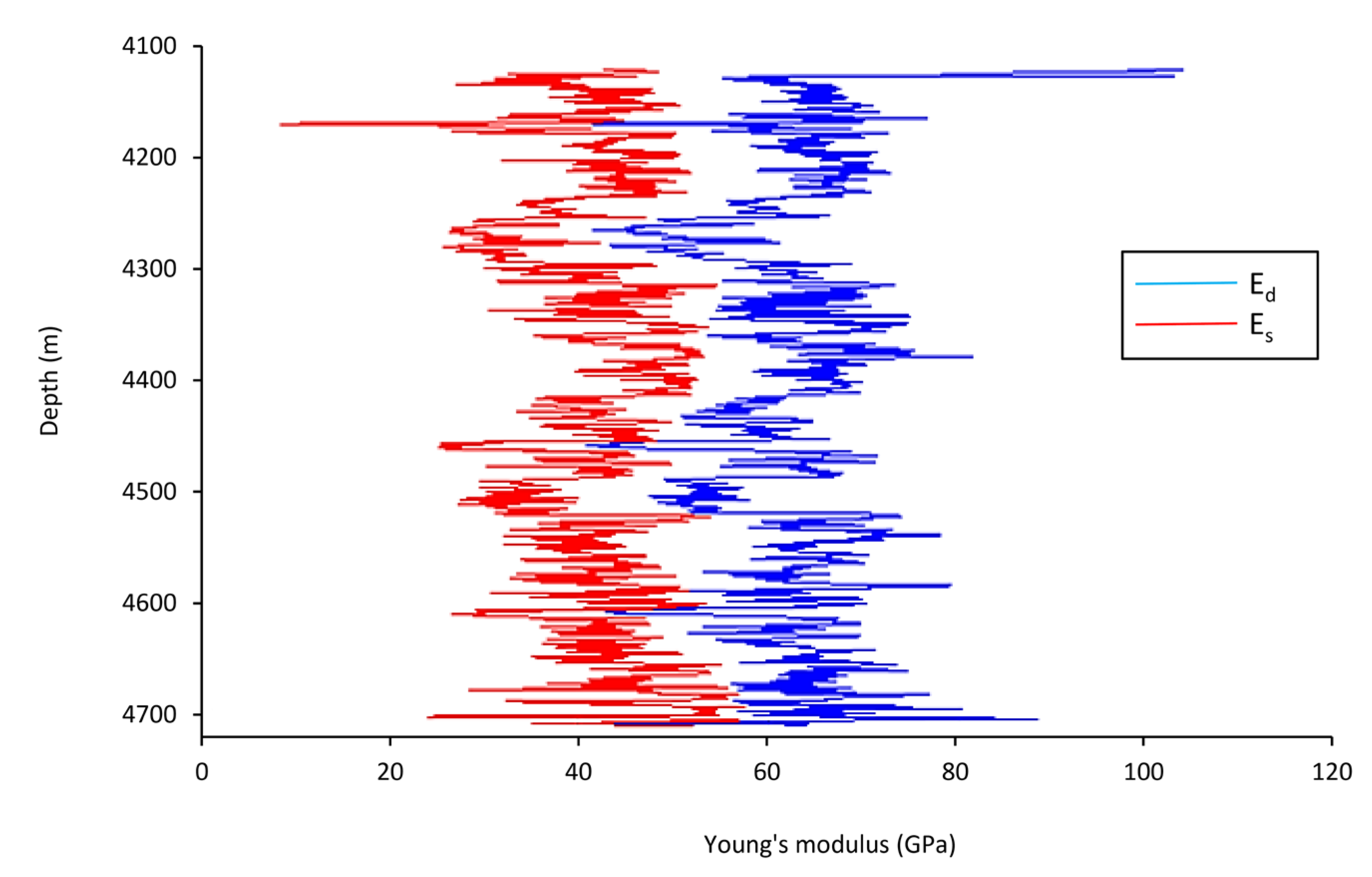
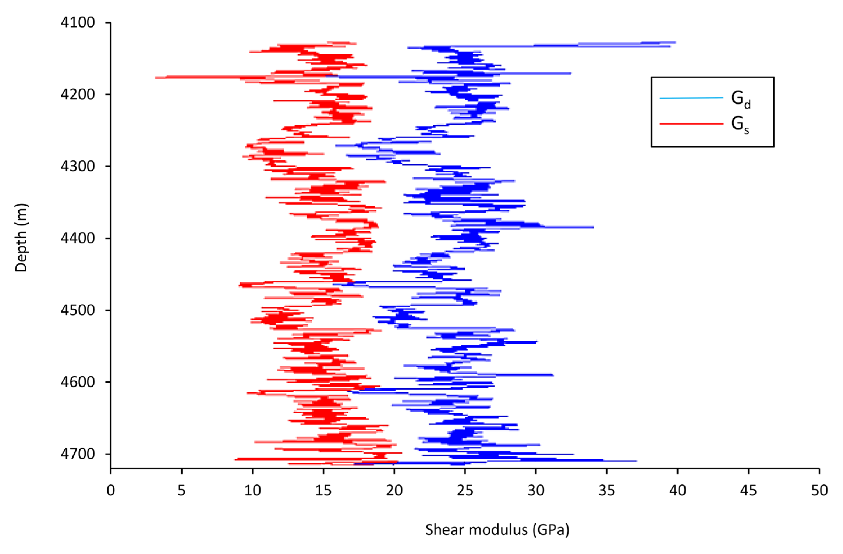
Despite all the efforts toward ensuring wellbore stability in recent years, the oil industry has several problems such as stuck pipes and lost circulation that lead to the collapse of wellbores. It is now well established from various studies that an appropriate plan is required to optimize drilling conditions, determine the MWW, and define the angle of deviation in terms of wellbore stability. Factors that influence drilling operations in underground formations are geo-mechanical factors such as in-situ stress and pore pressure, and mechanical properties such as Poisson’s ratio, Young’s modulus, and compressive strength [15]. A systematic understanding of how these factors impact wellbore instability can help determine the MWW in drilling operations. This particular research points to the need for obtaining the lower limit of the mud weight window and determining the optimal path of the wellbore when using directional drilling technology.

2. Numerical Modeling of Wellbore Stability

Several models of induced stress in a circular wellbore have been proposed, predicting the desirable mud pressure using 2D or 3D failure criteria. The linear elastic model is perhaps the most prevalent technique among the presented models. To predict borehole breakout, the Mohr–Coulomb failure criterion is frequently used, and is based on the concept that principal stresses of σ1 and σ2 rise in a linear manner during failure. By the way, there is no effect on rock strength from the intermediate principal stress of σ3.

Manshad et al. [16] applied some reliable analytical and numerical methods, e.g., Mohr–Coulomb and modified Lade, to calculate wellbore instability and estimate Iran’s MWW and drilling direction. The accuracy of mud pressure results is validated by the finite difference method and elastoplastic model and has demonstrated the highest MMP (minimum mud pressure) from the Mohr–Coulomb method. Manshad et al. [16] reported that an inclination of 20° is required to obtain the MMP for a wellbore. Yamamoto et al. [17] analyzed chemical and geomechanical data from the Zakum field’s shale instability in the UAE and concluded that drilling fluid and bedding plane are the main cause of wellbore instability. A geomechanical model is also used to predict wellbore instability and estimate in-situ pressures [18]. A necessary consequence of their study is the effect of wellbore inclination on breakout pressure. Waragai et al. [19] presented an operation guideline to eliminate the severity of wellbore instability in Nahr Umr shale formation in the offshore field in UAE after the prohibition of using diesel in water-based drilling mud. This study found that mechanical failure is imputed from the mud invasion into a lamination, and effective wellbore cleaning plays a significant role, especially with a wellbore angle between 30° and 50°. As a result of the guideline implementation, no wellbore with sidetracking has been noticed. Waragai et al. [19] inferred that the guideline works, and wellbore instability problems could be mitigated by following it. Han et al. [20] showed that a combination of tectonic movements and inappropriate MWW cause fractures on shale formation in the Phu Horm field and, therefore, the wellbore instability issue. As a suggestion, the drilling strategy can be modified while applying proper components and inhibitors to prevent the intrusion of drilling mud [21] into the fractures of underground formations.

Furthermore, a geo-mechanical model was applied by Alsubaih [22] to determine the ODMP in the Tanuma shale formation, Iraq. The results from 45 deviated wellbores showed that shear failure of wellbores causes the pipes to stick. In a study investigating the wellbore stability, Tutuncu et al. [23] reported that fundamental processes to prevent stuck pipes know about underground formations’ in-situ pressures and rock properties.

Moreover, Wang et al. [24] applied a two-dimensional (2D) finite-element model to simulate symmetrical fractures on the wellbore wall affected by anisotropic in-situ stresses and fracture length. By the way, the stress distribution is also calculated by considering fracture breadth before and after fracture bridging. However, in this numerical research, the leaking-off of fluid from the wellbore wall and fracture surface is neglected, given no information about fracture behavior after bridging and the effect of fluid inside the rock. Gomar et al. [25] used a finite-element model to assess the distribution of wellbore stress supported by the four failure criteria in terms of the wellbore wall’s stability. The results showed that a minimum MWW is required for wellbore stability. Chen et al. [26] examined a series of 3D heterogeneous tunnel models considering varying joint dip angles with the aim of understanding the zonal disintegration phenomenon. They found that zonal disintegration is induced by the stress redistribution of surrounding rock masses. Chen et al. [26] also realized that the model with a larger inclination angle is damaged further before the final collapse of the wellbore.

The literature on wellbore stability misses the importance of the wellbore’s deviation angle and azimuth. Concerning the availability of geo-mechanical data, this research investigates the optimization of the drilling route, i.e., the wellbore’s deviation angle and azimuth, in wellbore-D of the Azar oilfield, Iran. To this aim, a three-dimensional (3D) finite-element model in ABAQUS is simulated to analyze in-situ stresses and determine the MWW in the drilling operation of wellbore-D in the Azar oilfield. Drawing upon this strand of research into the appropriate plan, this research attempts to evaluate the mechanical properties of rock, elasticity modulus, properties of rock failure, pore pressure, and in-situ stress of wellbore in various deviation angles.

3. Materials and Methods

3.1. Modeling Analysis

A 3D finite-element numerical model was first applied by ABAQUS software, a powerful tool and perfect source of various elements to solve the issues in the geophysical model, to simulate a wellbore instability from the Sarvak Formation in the Azar oilfield, Ilam Province, Iran. Gomar et al. [25] stated that analytical solutions can be used for the distribution of principal stresses around a smooth circular wellbore wall. To better simulate the actual bottom wellbore conditions of lost circulation, the 3D finite-element model allows the simulation of wellbore circulation and fluid loss at the same time [27]. In a dynamic state, the 3D finite-element model was used to predict lost circulation with drilling mud in the Azar Oilfield’s wellbore-D and compute the principal stresses around the deviated wellbore. The model was then constructed by changing the deviation angle and wellbore extension to obtain the lower limit of the MWW. The analysis in ABAQUS consisted of three stages: pre-processing, processing, and post-processing. The discreteness of the geometric model was performed in the pre-processing stage, and appropriate elements were applied to compensate for limited components. Other stages were coded here in instructions known for software analytics. The instructions were then typed into Notepad as input files. In ABAQUS, this task is performed by ABAQUS/CAE. Figure 1 shows an overview of the stages by ABAQUS analysis.

3.2. Physical Properties of the Sarvak Formation

Petrophysical parameters of the Sarvak Formation, including porosity and density, were obtained from well-logs data. The amount of porosity changes with depth can be seen in Figure 2, and its average amount for the Sarvak Formation is 5.5%. The amount of bulk density was calculated for various formation depths by density log (Figure 3). The average density in the Sarvak Formation is 2.55 gr/cm³. Well test, the time recorded for production rate and wellbore pressure, was also conducted to determine the formation’s permeability. Measuring this parameter was obtained in the laboratory using the repeat formation tester (RFT) tool. The average permeability value in the X and Y directions is 0.84 mD and, in the Z direction, is 0.51 mD.

3.3. Mechanical Properties of the Sarvak Formation

Knowing about the rock mechanics plays a fundamental role in drilling. In this regard, two main factors should be considered, including in-situ pressures and the influence of fluid forces in the wellbore. In the case of deep-well drilling, the overburden pressure is considered as well. Poisson’s ratio (ν) is one of the main mechanical properties used to estimate wellbore stresses. The static value of Poisson’s ratio was obtained using the uniaxial compressive test on the cores taken from the Sarvak Formation, wellbore-D in the Azar oilfield. The dynamic value of Poisson’s ratio was obtained in the laboratory using an ultrasonic machine and acoustic log. In this study, the dynamic value of this parameter obtained from the acoustic log is as follows.

$$v=\frac{{\left(\frac{\mathsf{\Delta }{t}_s}{\mathsf{\Delta }{t}_c}\right)}^2-2}{2\left({\left(\frac{\mathsf{\Delta }{t}_s}{\mathsf{\Delta }{t}_c}\right)}^2-1\right)}=\frac{V_p^2-2V_s^2}{2\left(V_p^2-V_s^2\right)}$$

(1)

From Equation (1), $\mathsf{\Delta }{t}_c$ is the pressure wave time in microsecond per foot (μs/ft) and $\mathsf{\Delta }{t}_s$ is the shear wave time in μs/ft. Vp and Vs are the velocities of P and S waves, respectively, in km/s. In the study area, as shown in Figure 4, the average dynamic value of Poisson’s ratio is about 0.32.

Also, the achievement process of Young’s modulus in both static (E_s) and dynamic (E_d) states is similar to Poisson’s ratio. The E_d value was calculated from Equation (2).

$$E_d=\frac{{\rho }_b}{\mathsf{\Delta }{t}_s{}^2}\left(\frac{3\mathsf{\Delta }{t}_s{}^2-4\mathsf{\Delta }{t}_c{}^2}{\mathsf{\Delta }{t}_s{}^2-\mathsf{\Delta }{t}_c{}^2}\right)\times 1.34\times {10}^{10}$$

(2)

From Equation (2), ${\rho }_b$ is the density (gr/cm³). In the study area, as shown in Figure 5, the value of E_s is 41.5 GPa.

Furthermore, the shear modulus was achieved by sonic and density logs. The static value of shear modulus was calculated from Young’s modulus and Poisson’s ratio. Figure 6 shows dynamic and static shear modulus in the Sarvak Formation with an average static shear modulus of 14.8 GPa.

$$G_d={\rho }_b\left(\frac{1}{\mathsf{\Delta }{t}_s^2}\right)\times 1.34\times {10}^{10}$$

(3)

Moreover, the uniaxial compressive strength (UCS) of the Sarvak Formation in the Azar oilfield was calculated in the laboratory. Figure 7 shows the UCS’s static value of the Sarvak Formation at depths from 4100 m to 4720 m. The UCS’s static value was obtained from the uniaxial compressive strength test with an average value of 79.2 MPa.

Besides, the amounts of cohesion and friction angle for the Sarvak Formation were obtained from triaxial compressive strength data with an average amount of 2.72 MPa and 40°, respectively. In doing so, the tensile strength of the Sarvak Formation was used for calculating the tensile failure in the well’s wall due to stress concentration. The tensile strength of a rock type, about $\frac{1}{8}$ to $\frac{1}{12}$ UCS [28], can be measured via the Brazilian tensile strength test. In this study, the average amount of the Brazilian tensile strength test was 8.57 MPa. Furthermore, Biot’s coefficient describes how much of the total stress and pressure changes get converted to effective stress [29]. Biot’s coefficient measures the ratio of the fluid volume squeezed out to the volume change of the rock if the latter is compressed while allowing the fluid to escape. Biot’s constant is a complex function of several parameters, including porosity, permeability, grain sorting, and confining pressure. A more practical and affordable method uses sonic log and core data to calculate dynamic Biot’s coefficient through Equation (4), where K_s and K_min are bulk and grain modulus, respectively.

$$\alpha =1-\left(\frac{K_s}{K_{min}}\right)$$

(4)

4. Stress Analysis Results

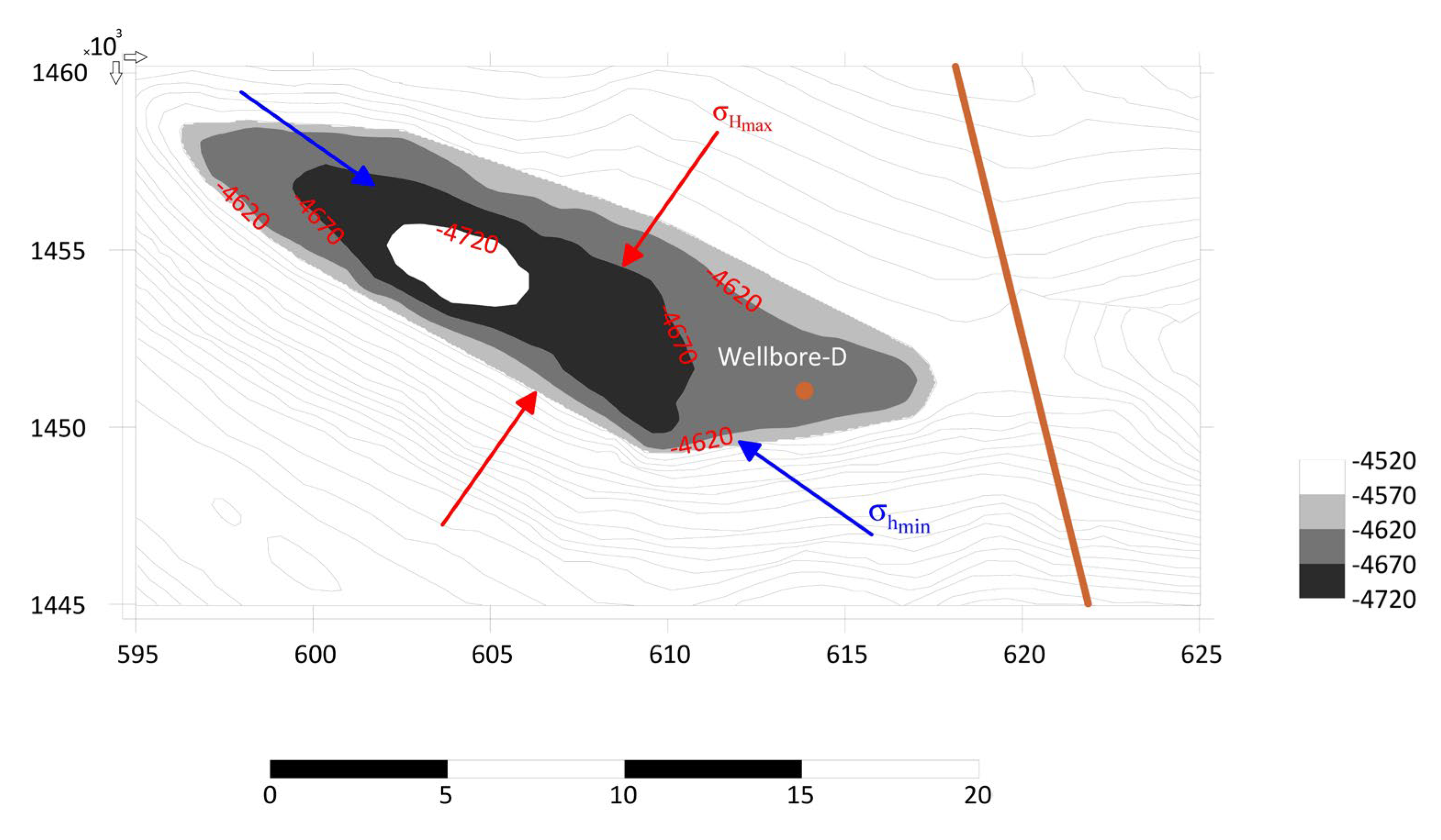
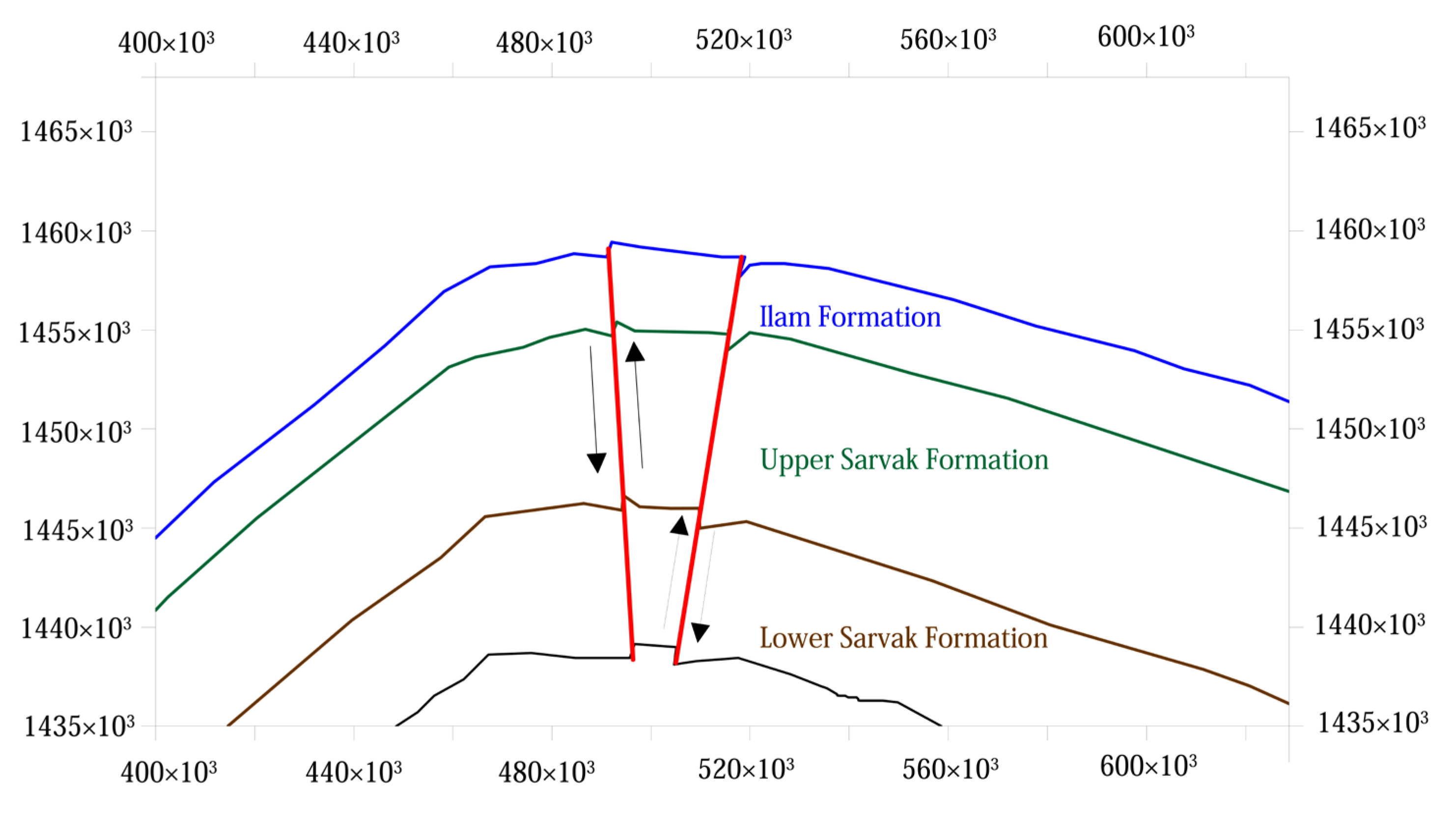
The stress analysis results from Figure 8 and Figure 9 show that the Azar oilfield is structurally under the impact of a complex tectonic system, dominated by two reverse faults representing a pressure system, especially across the Sarvak Formation. There is a perpendicular fault near the Azar oilfield, which no longer exists after the Asmari Formation. As per Figure 8, the direction of minimum and maximum horizontal stresses is according to the reverse fault’s configuration (σ_H > σ_h > σ_v) in the Azar oilfield. This configuration caused a horst in the central part of the Azar oilfield (Figure 9).

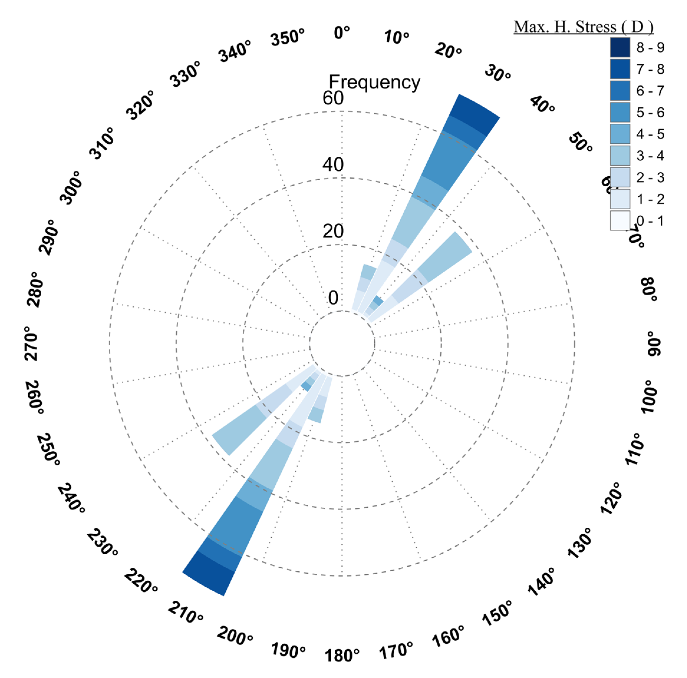
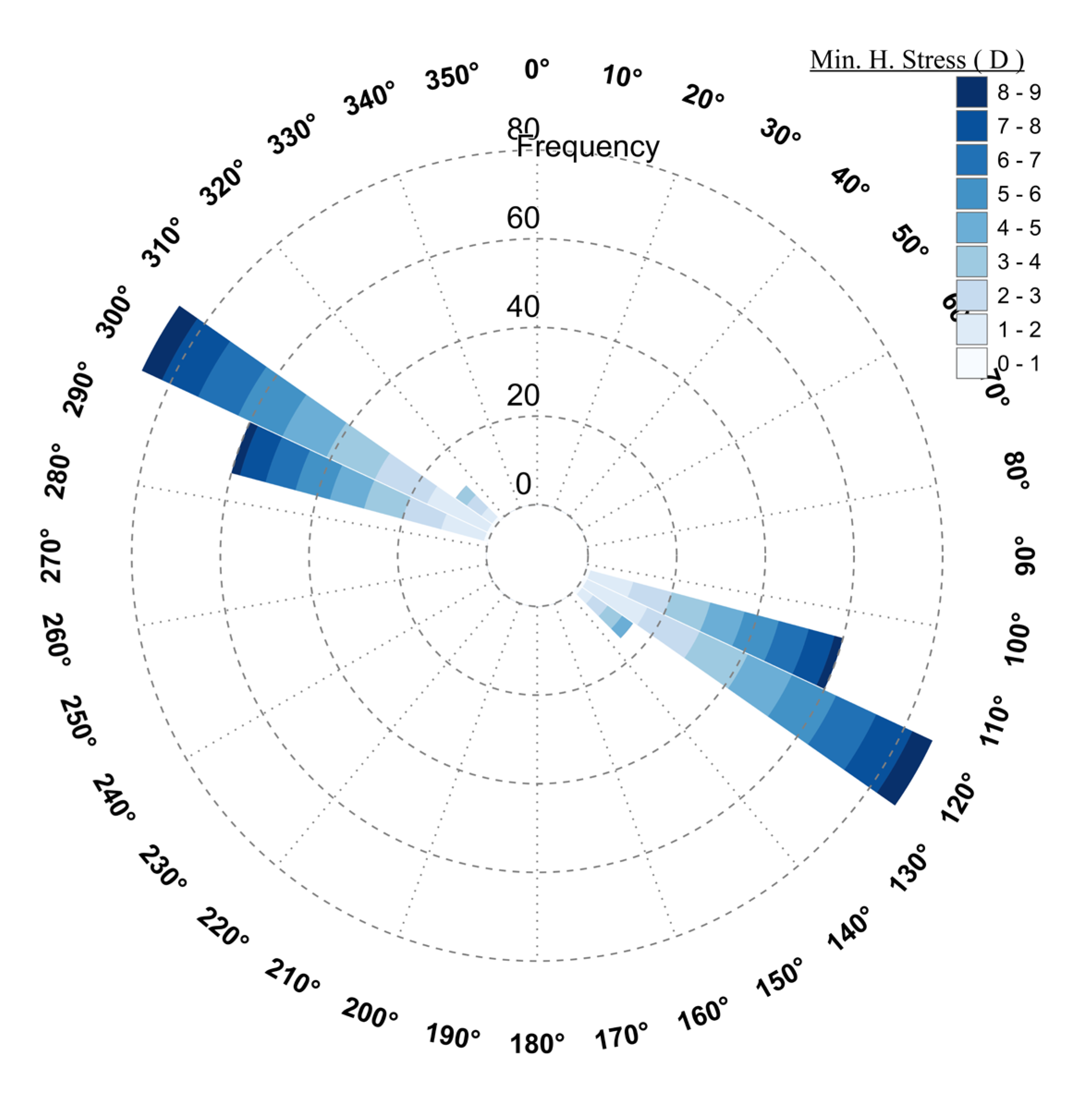
From the results of well instability analysis as a rose diagram (Figure 10), σ_H and σ_h are directed at N30° E and N60° W, respectively. Inclination angles of 15°, 30°, 60°, and 90° are represented by circles with different radii. Each circle has 360°, representing azimuth angles of wellbores. The minimum mud density (MMD) values in g/cm³ are shown in a color bar on the right side of the rose diagram. In this example, at a certain depth, for a wellbore with an inclination degree of 45° and an azimuth angle of N30° E, the MMD is 1 g/cm³. One point to be noted in the hemisphere plot of the MMD is that all values are to avoid wellbore collapse or shear failure. Besides, the wellbore pressure is higher than the formation pore pressure to avoid a drilling kick [30]. In the literature, the lower bound of the mud window is the minimum mud weight required to achieve the desired degree of wellbore stability. In this study, normal pore pressure is 1.01 g/cm³, and therefore, the lower bound of MMW is the pore pressure plus the maximum swab pressure to avoid the drilling kick, rather than the MMD to avoid the wellbore collapse.

Figure 10 and Figure 11 show rose diagram results of wellbore-D in the Azar oilfield. According to the results, induced tensile fractures occur in azimuth 30° and 210° of NE–SW, indicating the direction of maximum horizontal stress (Figure 10). In contrast, the wellbore collapse in azimuth 120° and 300° shows the direction of minimum horizontal stress (Figure 11).

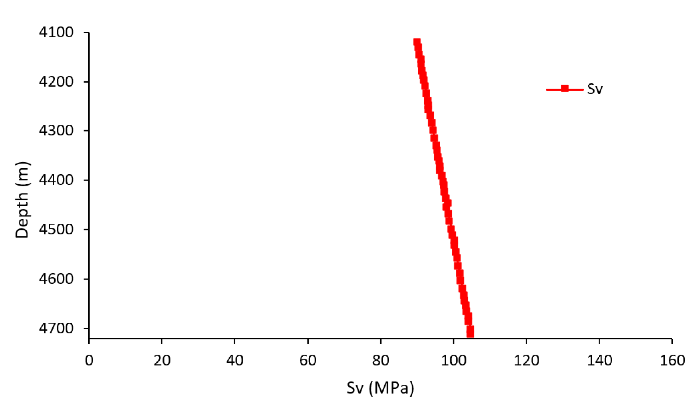
The literature revealed that the issue of wellbore instability is referred to the mechanism of principal stresses [31,32], while the role of in-situ stresses is mainly neglected. In this study, the amount of in-situ stresses was determined to cover all mechanisms involved in the wellbore instability of the Azar oilfield. In this regard, overburden pressure or vertical stress $\left(S_v\right)$ in an arbitrary depth of wellbore equals the weight of overburden above this depth. So, the vertical stress of wellbore-D in the Azar oilfield was obtained from Equation (5).

$$S_v={{\displaystyle \int }}_0^z\rho \left(z\right)gdz=\overline{\rho }gz$$

(5)

where $\rho \left(z\right)$ shows density as a function of depth ($z$), Earth’s gravity acceleration ($g$), and average density of overburden layers ($\overline{\rho }$). Also, Equation (6) was proposed for offshore drilling operations in which a column of water exists above the formation.

$$S_v={\rho }_{w}g{z}_w+{{\displaystyle \int }}_{z_w}^z\rho \left(z\right)gdz\approx {\rho }_{w}g{z}_w+\overline{\rho }g\left(z-z_w\right)$$

(6)

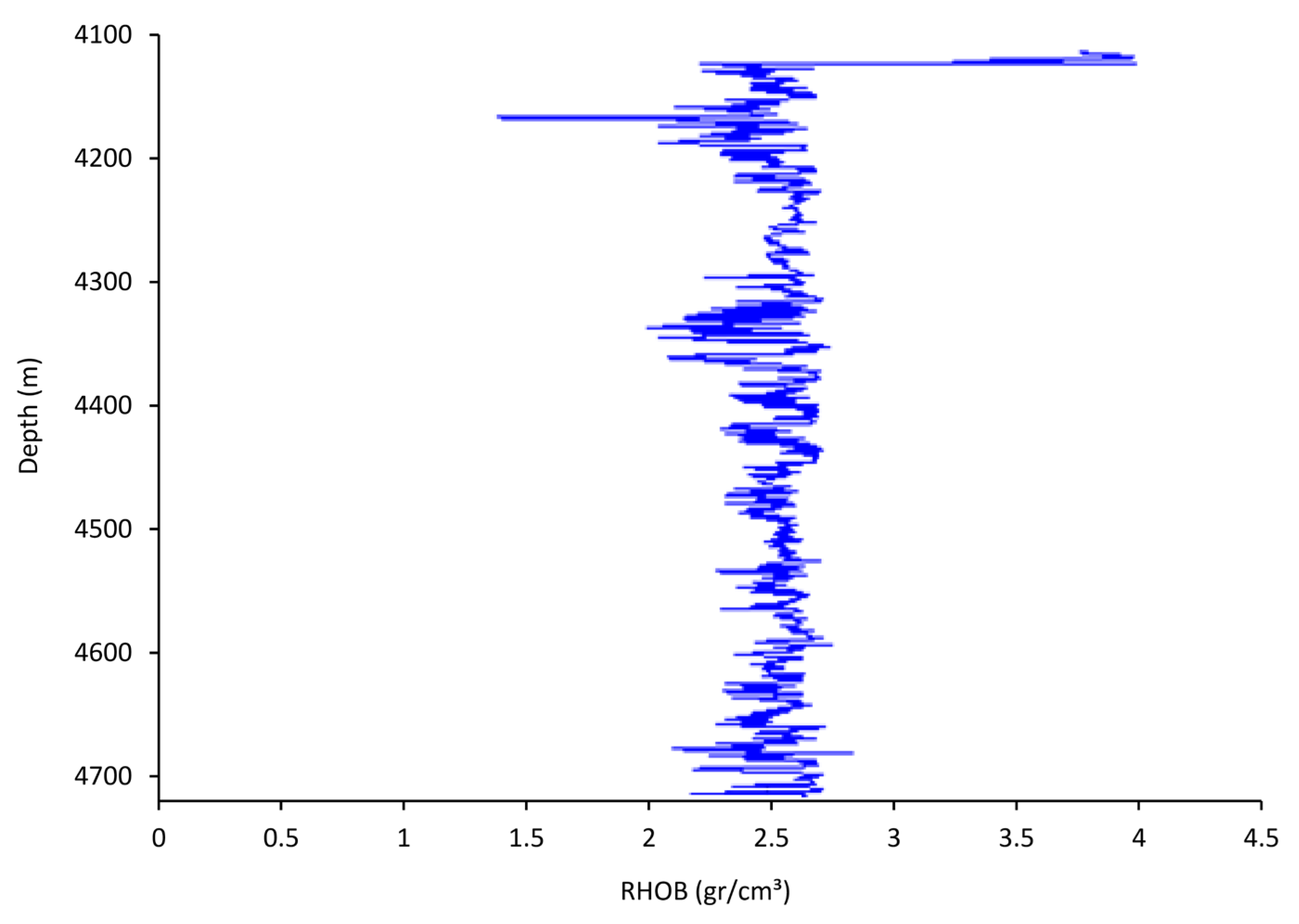
where ${\rho }_w$ denotes the density of water and $z_w$ is the depth of water. The water density was assumed to be 1.03 gr/cm³ [31]. Due to the high cost of using the well-logging method, data collection is usually associated with a range of hydrocarbons contained, and routinely, there are sections in the upper parts of the wellbore where log-recording activities have not been performed. Hence, the density of these sections in the formation was assessed by the linear interpolation of data obtained from well logs. 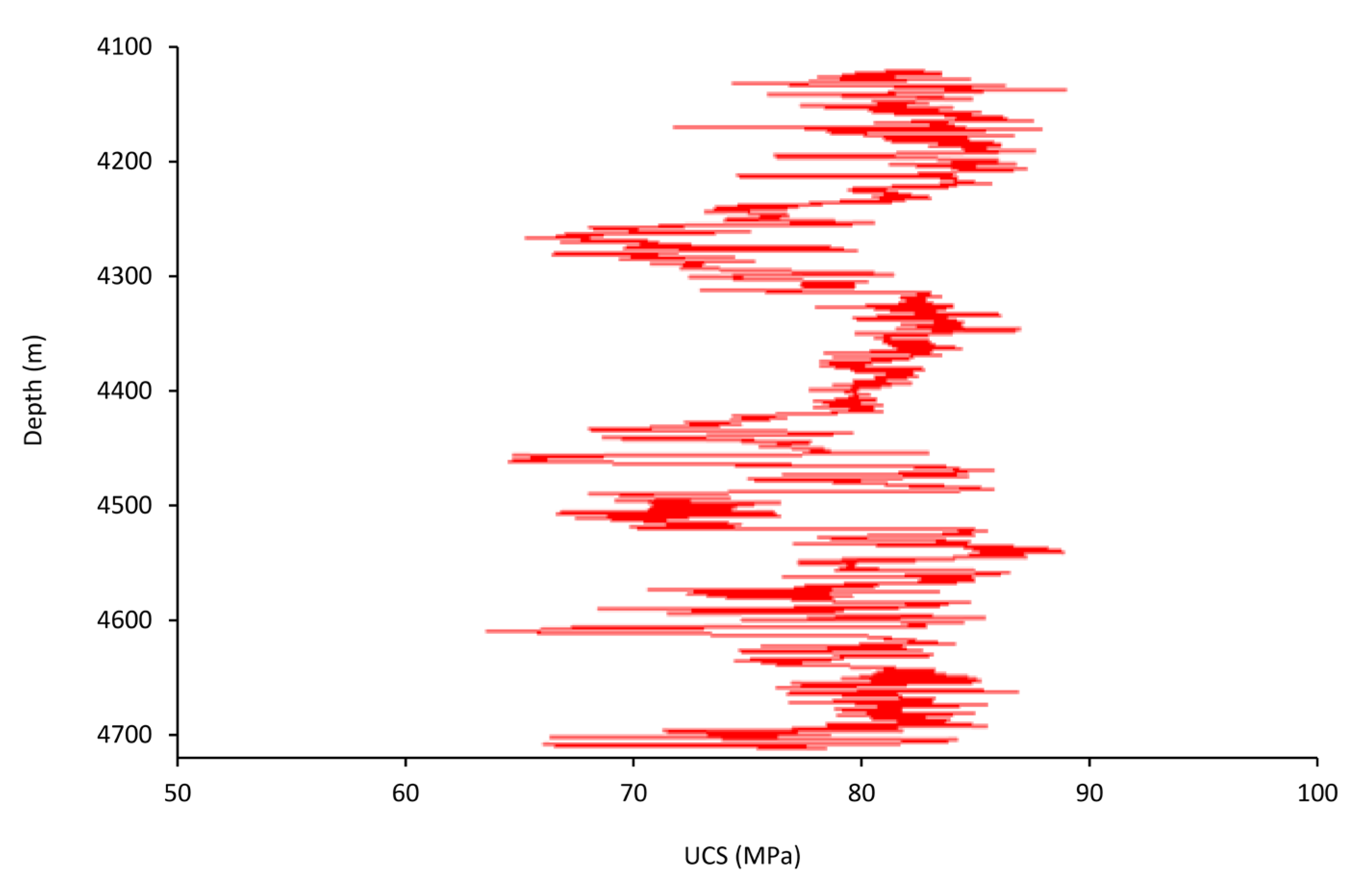In this study, an average density of about 2.3 gr/cm³ was considered for the Sarvak Formation. From Figure 12, the $S_v$ value for the depth of 4400 m is 99.17 MPa.

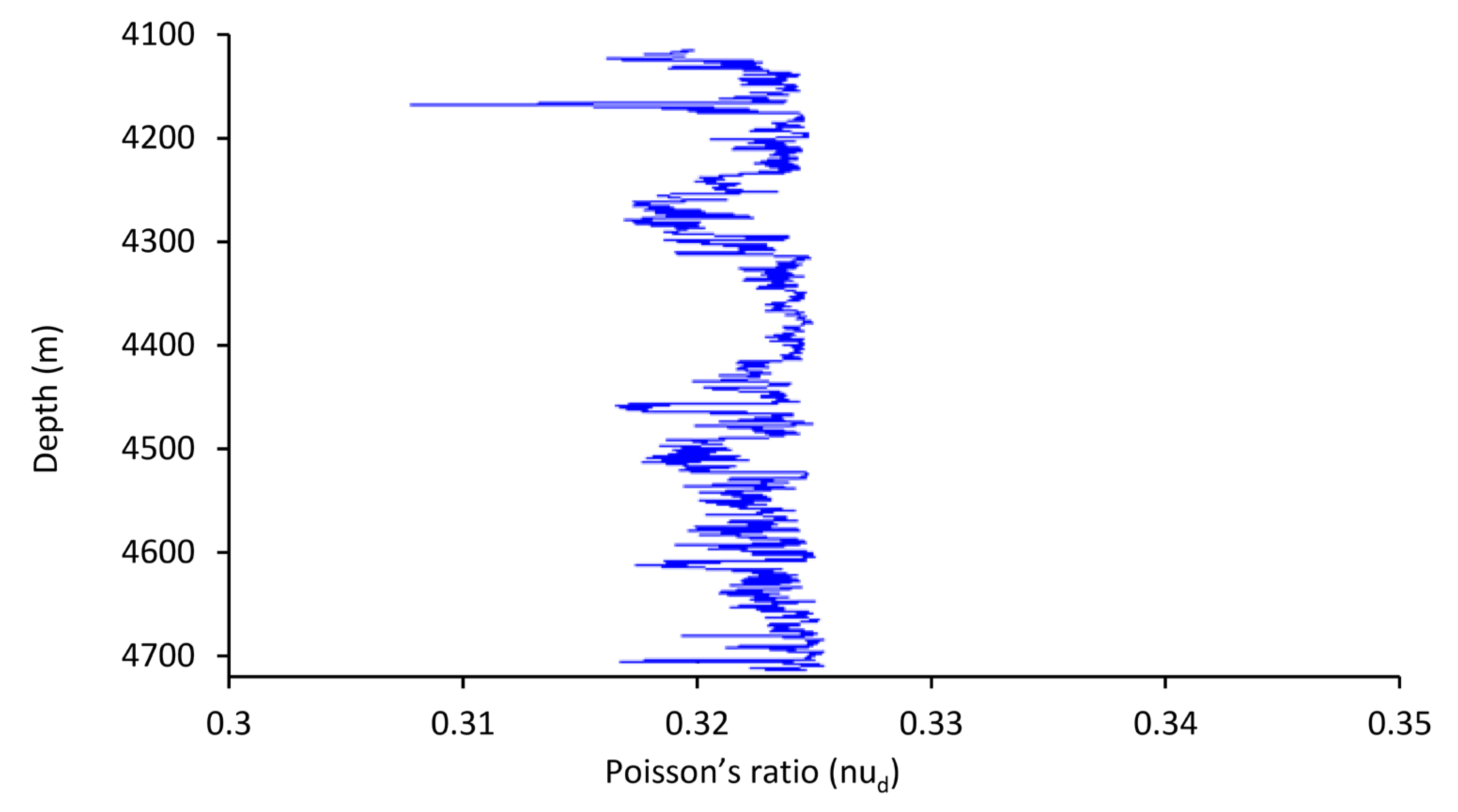
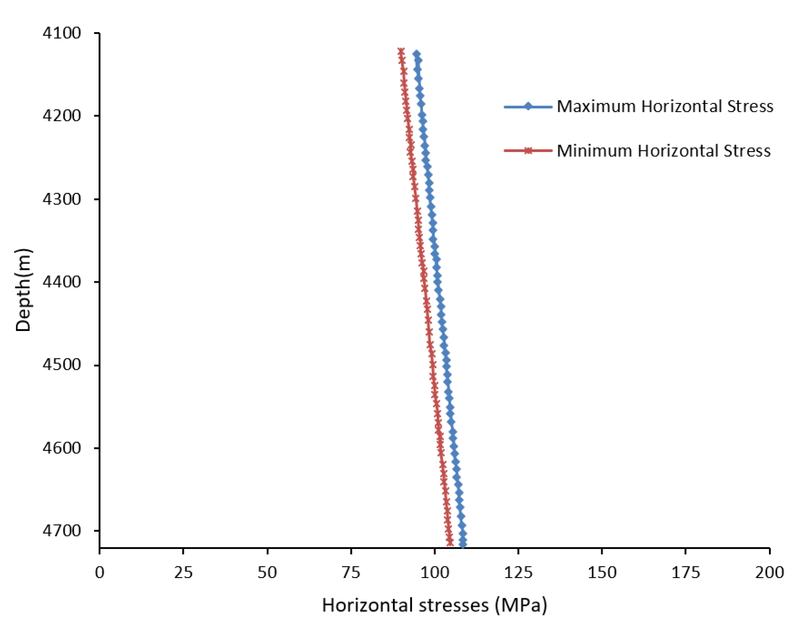
Moreover, existing pore pressure recognizes its critical role in the distribution of stress in wellbores. Equations (7) and (8) present the minimum ($S_h$) and maximum ($S_H$) horizontal stress values.

$$S_h=\frac{\nu }{1-\nu }\left(S_V-\alpha P_p\right)+\alpha P_P+\frac{E}{1-{\nu }^2}{\epsilon }_x+\frac{\nu E}{1-{\nu }^2}{\epsilon }_y$$

(7)

$$S_H=\frac{\nu }{1-\nu }\left(S_V-\alpha P_p\right)+\alpha P_P+\frac{\nu E}{1-{\nu }^2}{\epsilon }_x+\frac{E}{1-{\nu }^2}{\epsilon }_y$$

(8)

In these equations, V is Poisson’s ratio, $\alpha$ is the Biot’s coefficient, $P_p$ is the pore pressure, ${\epsilon }_x$ and ${\epsilon }_y$ are respectively the strain indicator in the direction of the minimum and maximum horizontal stress, and sentence $S_V-\alpha P_p$ is recognized under the title of effective vertical stress. As there is no result of the leak-off test (LOT) in the Azar oilfield, parameters ${\epsilon }_x$ and ${\epsilon }_y$ are calculated using a trial-and-error method. The results from these strain parameters showed that the stress regime would be in reverse regime (i.e., $S_V\le S_h\le S_H)$. 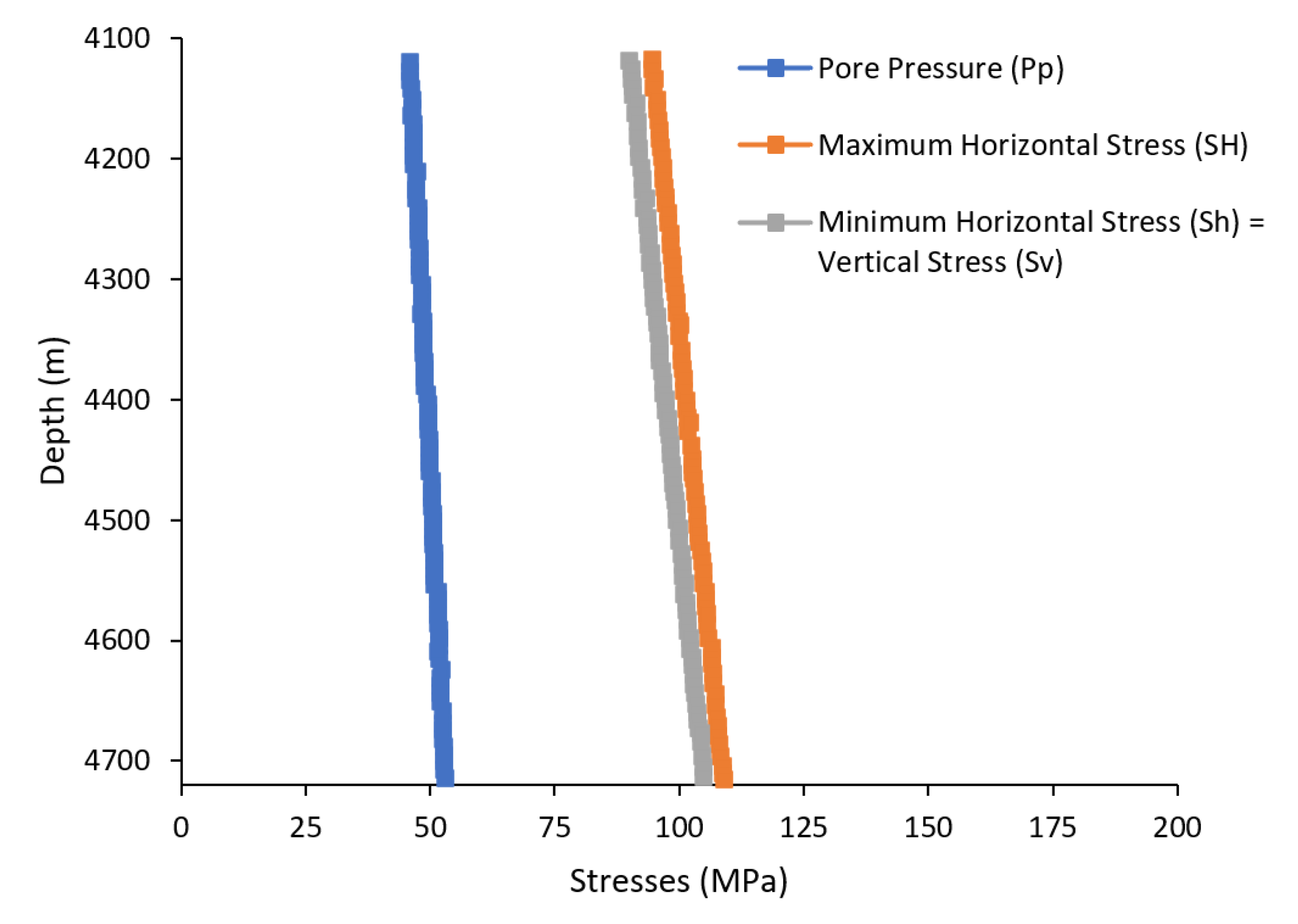So, the minimum horizontal stress amount equals vertical stress, and therefore, the proportion of the maximum horizontal stress towards vertical stress is 1.05 (Figure 13).

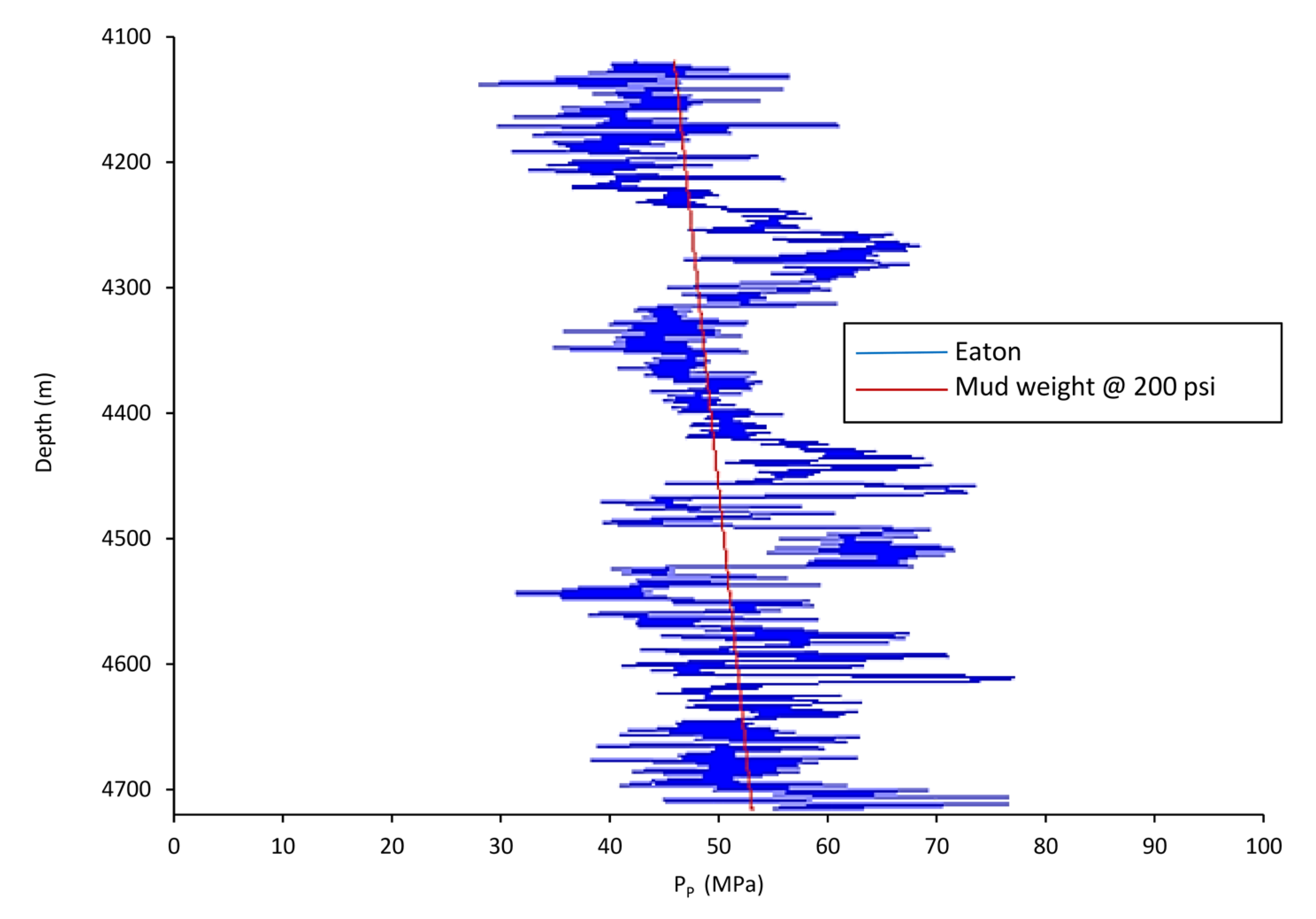
Furthermore, Eaton’s equation was applied to determine the amount of pore pressure in the wellbore-D of the Azar oilfield. The data reported here appear to support the assumption that the drilling operation is in an ultra-balance condition with a mud pressure of 200 pounds per square inch.

$$P_{pg}=OBG-\left(OBG-P_{ng}\right){(\frac{\mathsf{\Delta }{t}_m+\left(\mathsf{\Delta }{t}_{ml}-\mathsf{\Delta }{t}_m\right)e^{-cZ}}{\mathsf{\Delta }t})}^3$$

(9)

In Equation (9), OBG and $P_{ng}$ are the overburden and hydrostatic pressure gradients, respectively. $\mathsf{\Delta }t, \mathsf{\Delta }{t}_m$, and $\mathsf{\Delta }{t}_{ml}$ are the sonic compressional transit time (DTC) of formation, rock matrix, and mudline, respectively. Z and c denote the depth and compaction constant, respectively. Figure 14 illustrates pore pressure changes from Eaton’s equation and mud pressure in the wellbore-D of the Azar oilfield. As shown in Figure 14, the pore pressure gradient of the Sarvak Formation is about 11.5 MPa/km.

Figure 15 represents the results of in-situ stresses (i.e., the vertical, minimum, and maximum horizontal stress) and pore pressure obtained from wellbore-D of the Azar oilfield.

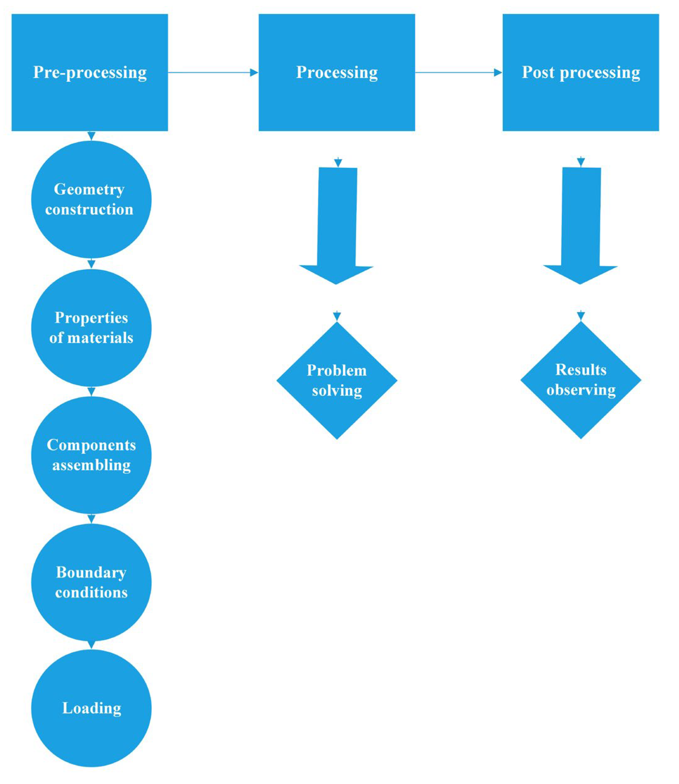
4.1. 3D Model’s Geometry

The first phase of the 3D model construction is the creation of intended geometry, including a block of porous media with a well diameter of 17.78 cm (7 inches). Dimensions of the constructed model are 583 × 400 × 583 cm. Since this study aims to determine the optimal route for drilling operations in the Azar oilfield, changes in the deviation angle or curvature beam should be considered. Figure 16 illustrates a schematic view of the 3D model from the wellbore-D in the Azar oilfield. At first, the wellbore is vertical, and then it deviates from the vertical state with a 15-degree slope per 100 ft.

At last, the wellbore finds a horizontal state. With the porosity and fluid in rocks, the modeling analysis moved further to the depths and caused changes in the geo-mechanical behavior of the Sarvak Formation. On the other hand, an elastic model with no consideration of porosity and pore fluid creates a hypothesis with an immense error in understanding the process. This is because pore spaces [33], pore fluids, and their connection within the wellbore play a crucial role in addressing the issues of the drilling operation. In this regard, lack of porosity causes an increase in shear and tensile strengths, resulting in an invalid outcome.

The top part of the model was located at a depth of 4000 m. In this field, the value of vertical stress resulting from the overburden weight at a depth of 4000 m is 90.15 MPa in the Z direction. The estimated minimum and maximum horizontal stresses are 90.15 MPa and 94.66 MPa, respectively. In other words: $K_h=\frac{{\sigma }_h}{{\sigma }_v}=1$ and $K_H=\frac{{\sigma }_H}{{\sigma }_v}=1.05$. Also, pore pressure is 46 MPa, and the pore pressure gradient is 11.5 MPa/km.

4.2. Boundary Conditions and Modeling Steps

The boundary conditions of a numerical model include variables such as stress and displacement. If in the intended model the behavior of a material is elastic, the grid boundary distance to the center of mode from each side will be five times more than the dimensions of the model range, which is considered the highest amount in this study due to the poroelastic behavior of the material [25,34]. In the constructed models, the plates perpendicular to the coordinate axis have zero displacement, and the model’s surface has zero displacement along with the z-axis. Also, the circumstances of pore pressure on the external zones of models have been applied. By applying the initial conditions, the strata condition was simulated. In an ideal situation, information about in-situ stresses was obtained from the in-situ measurements in the Azar oilfield.

In the Azar oilfield, the pore pressure element of C3D8P, 8-node trilinear displacement, and pore pressure were used from ABAQUS by considering the freedom degree of pore pressure and 3D model. The shape of this element was categorized in the hexagonal type with a structured form of the mesh-scaling method. It is noteworthy that the mesh scaling’s size is partly changed and is finer, close to the wellbore, with no impact on the amount and distribution of displacements and stresses. In this numerical model, the elements and nodes are 26,957 and 29,738, respectively.

Moreover, there were two main phases in the proposed 3D model, including a geostatic step, creating a primary balanced model, and a drilling step. In the geostatic step, changing the shape and displacement of the model was negligible, and all initial conditions, including in-situ stresses, volumetric forces, boundary conditions, and pore pressure, were defined. In the drilling step, while drilling the wellbore, the number of stresses and displacements was increased in the wellbore-D. After the drilling operation, mud pressure was applied to the wellbore, resulting in a balance in changing the number of stresses and plastic strain in the wellbore wall. Since the regime stress is in the reverse state, the suitable azimuth for drilling accords maximum horizontal stress. Also, minimum mud pressure was related to the stability of the wellbore.

4.3. Verification Analysis of 3D Model

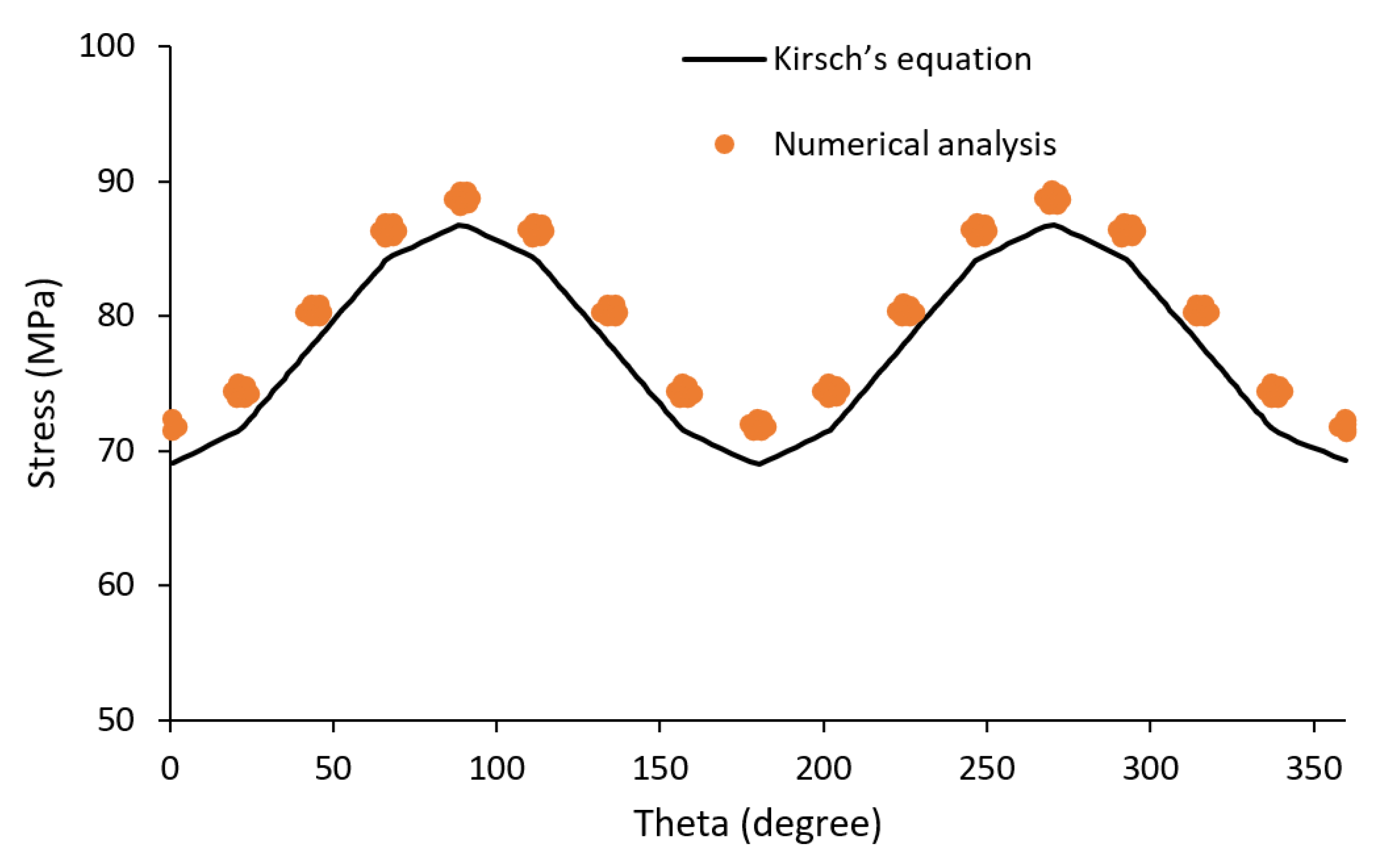
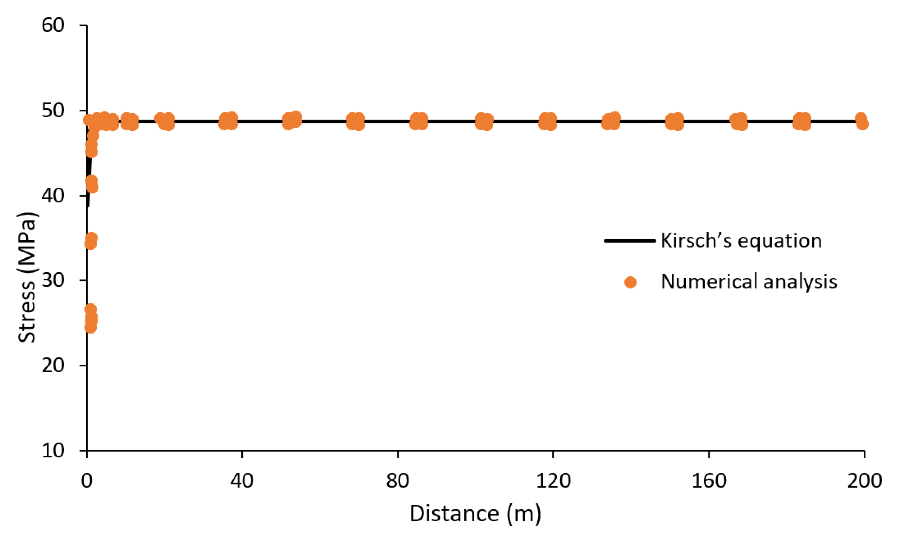
There were two stages that the proposed 3D model considers for modeling the drilling route in the wellbore-D of the Azar oilfield, including the azimuth of the wellbore in the directions of maximum and minimum horizontal stress. Analytical relations of Kirsch’s equation were applied to validate the numerical modeling process. These analytical relations can determine the distribution of stresses around the wellbore. 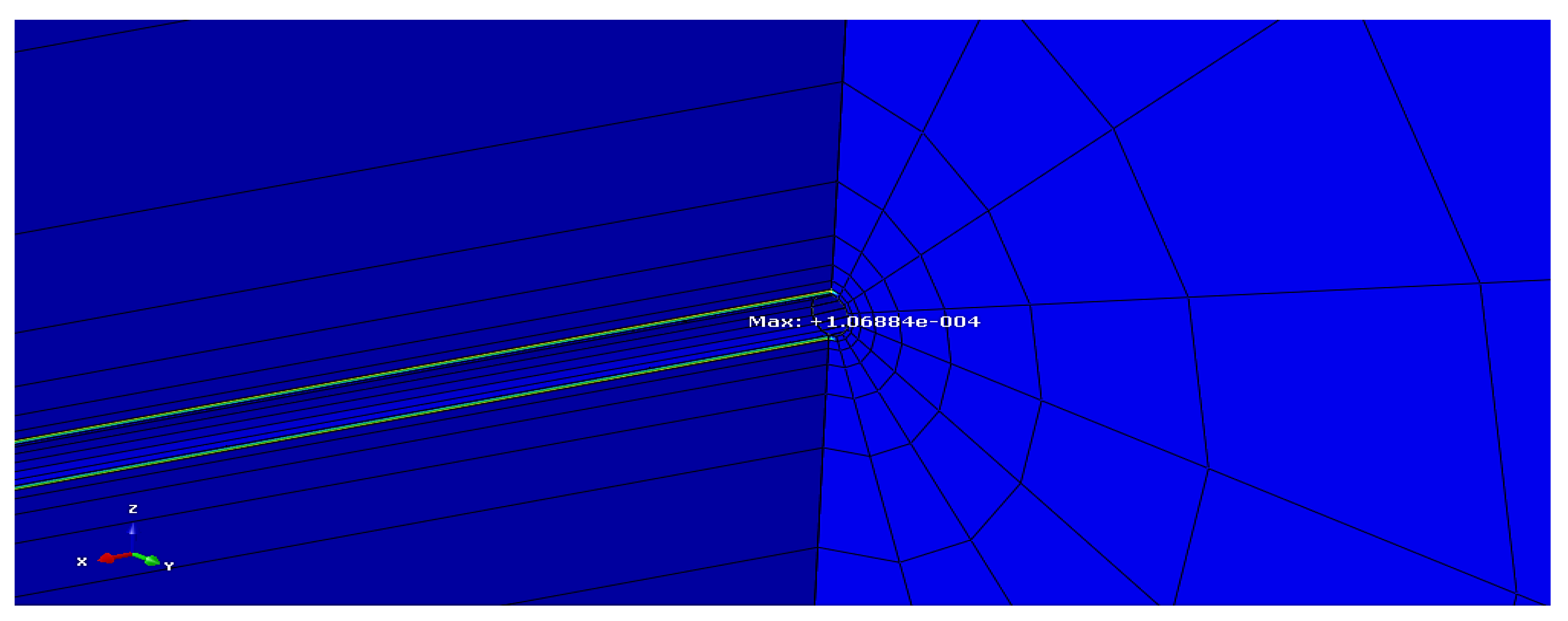Figure 17 and Figure 18 show the radial and axial stress distribution, respectively, around the wellbore-D in the Azar oilfield. The results indicated a good agreement between the numerical modeling and analytical solution with a modeling error of < 4%.

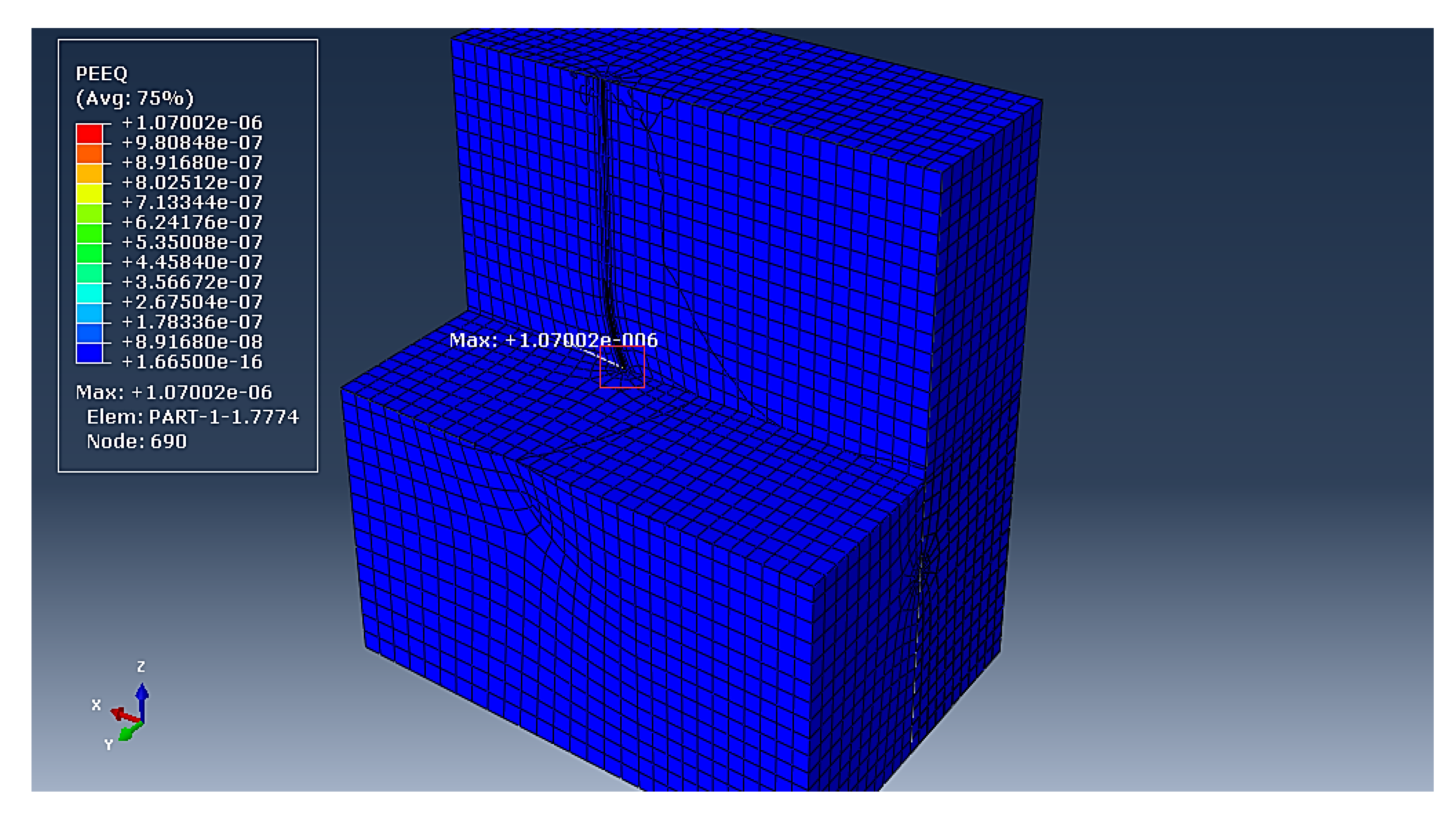
The modeling evidence on wellbore instability revealed that applying higher mud pressure leads to no shear failure in the wellbore-D’s wall. Incidentally, the lower limit of the mud window was determined to prevent any downfall of the wellbore-D’s wall in the Azar oilfield. ABAQUS modeling results showed that the lower limit of the MWW is 89 pcf. As indicated in Figure 19, a value lower than the MWW leads to a shear failure around a 10-degree deviation angle of the wellbore wall. Taken together, these results support the notion that the drilling operation in the Sarvak Formation caused a downfall of the wellbore-D with the approximate MMW of 75 pcf.

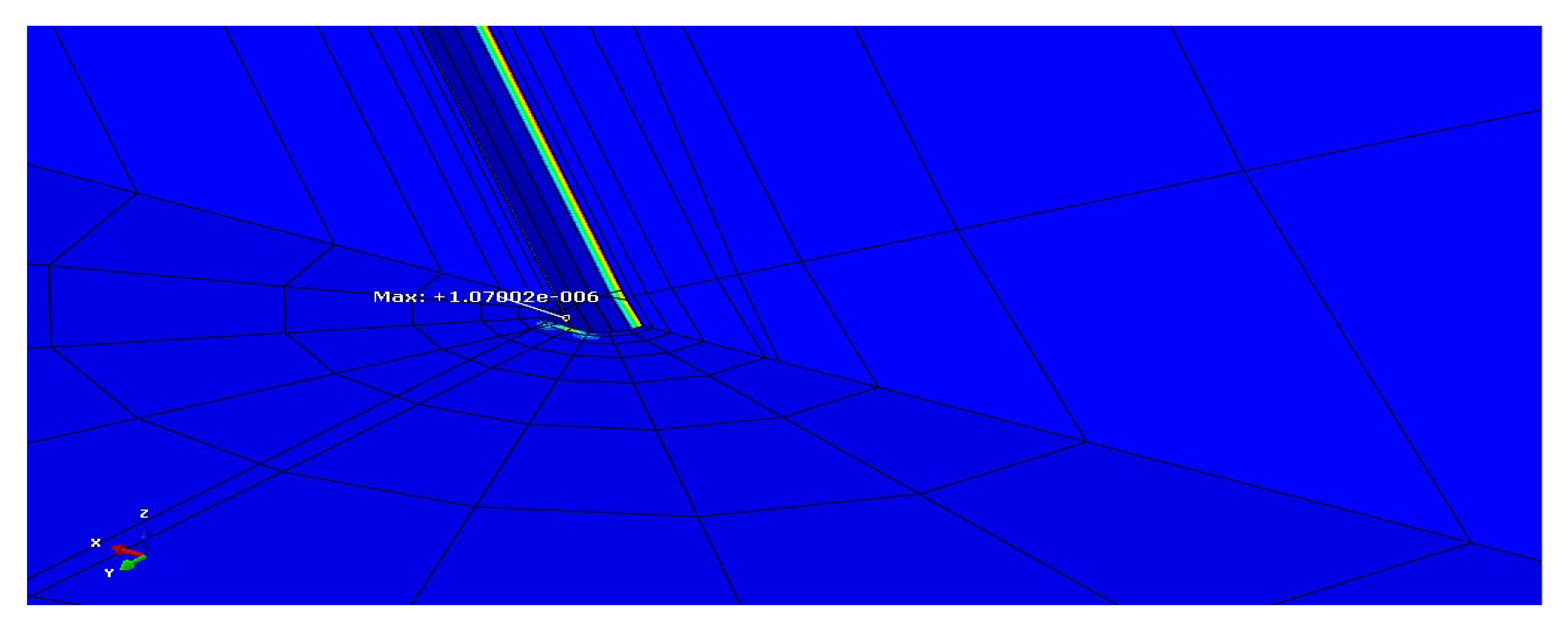
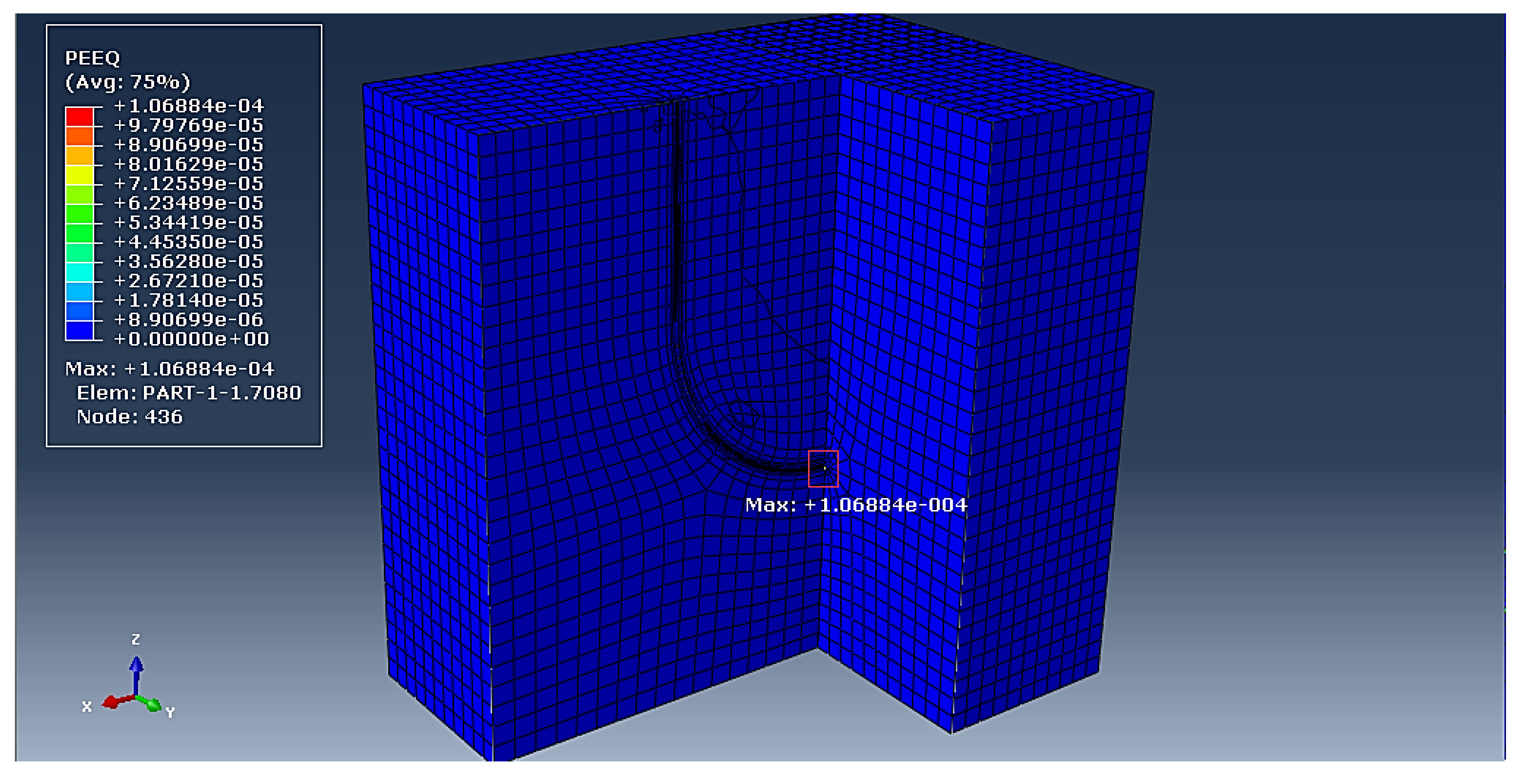
Also, Figure 20 presents starting the plastic zone in the horizontal wellbore at a mud pressure less than the MWW. In this case, the lower limit of the MWW is 90.3 pcf. As a result, a shear failure occurs in the deviation angle of 90°. Therefore, drilling the wellbore with the azimuth of maximum horizontal stress requires less mud weight, which lessens the cost of the drilling operation. Together, these results follow essential aspects from the analysis performed before the modeling that points to the reverse and strike-slip faults regime in the Azar oilfield. It can be considered as the most appropriate azimuth for maximum horizontal stress with the slightest dispute.

5. Conclusions

Wellbore instability is one of the main issues in oilfields while drilling an angular oil well. Determining the mud weight window is a practical solution for controlling wellbore instability. This study aimed to calculate the lower limit of the mud weight window in the Azar oilfield’s wellbore-D. The first set of analyses referred to constructing a 3D model with the finite element method. In this method, characteristics of a porous media, including porosity, permeability, pore pressure, percentage of saturation, and specific weight, were represented. The 3D finite-element model in ABAQUS was designed to determine the modeling and analysis solution for the wellbore’s deviation angle and azimuth in the Azar oilfield. The optimization of the drilling route was investigated to analyze in-situ stresses and determine the MWW in drilling operations. Kirsch’s equation was used to validate numerical modeling. Analytical relations of Kirsch’s equation showed an acceptable error to validate the numerical modeling process. The results showed that the drilling wellbore in the direction of the maximum horizontal stress needs lower mud weight compared to the direction of the minimum horizontal stress. In short, it can be stated that the active stress regime is a pressure system in the Azar oilfield that has created a combination of reverse and strike-slip faults throughout the structure. It is a prominent finding from this analysis that lower mud weight would reduce the cost of the drilling operation. Besides, these achievements on the wellbore instability would help us establish greater accuracy on this matter and provide valuable insights into the drilling of wellbores in petroleum engineering.

References

1. Das, B.; Chatterjee, R. Wellbore stability analysis and prediction of minimum mud weight for few wells in Krishna-Godavari Basin, India. Int. J. Rock Mech. Min. Sci. 2017, 93, 30–37. [Google Scholar] [CrossRef]
2. Ganguli, S.S.; Sen, S. Investigation of present-day in-situ stresses and pore pressure in the south Cambay Basin, western India: Implications for drilling, reservoir development and fault reactivation. Mar. Pet. Geol. 2020, 118, 104422. [Google Scholar] [CrossRef]
3. Karakosta, K.; Mitropoulos, A.C.; Kyzas, G.Z. A review in nanopolymers for drilling fluids applications. J. Mol. Struct. 2021, 1227, 129702. [Google Scholar] [CrossRef]
4. Aslannezhad, M.; Manshad, A.K.; Jalalifar, H. Determination of a safe mud window and analysis of wellbore stability to minimize drilling challenges and non-productive time. J. Pet. Explor. Prod. Technol. 2016, 6, 493–503. [Google Scholar] [CrossRef] [Green Version]
5. Sahu, C.; Kumar, R.; Sangwai, J.S. Comprehensive review on exploration and drilling techniques for natural gas hydrate reservoirs. Energy Fuels 2020, 34, 11813–11839. [Google Scholar] [CrossRef]
6. Awal, M.R.; Khan, M.S.; Mohiuddin, M.A.; Abdulraheem, A.; Azeemuddin, M. A new approach to borehole trajectory optimisation for increased hole stability. In Proceedings of the SPE Middle East Oil Show, Manama, Bahrain, 17–20 March 2001. [Google Scholar] [CrossRef]
7. Ibrahim, A. A review of mathematical modelling approaches to tackling wellbore instability in shale formations. J. Nat. Gas Sci. Eng. 2021, 89, 103870. [Google Scholar] [CrossRef]
8. Rahimi, R. The effect of using different rock failure criteria in wellbore stability analysis. Master’s Thesis, Missouri University of Science and Technology, Rolla, MO, USA, 2014. [Google Scholar]
9. Rahimi, R.; Nygaard, R. Comparison of rock failure criteria in predicting borehole shear failure. Int. J. Rock Mech. Min. Sci. 2015, 79, 29–40. [Google Scholar] [CrossRef]
10. Mehrabian, A.; Jamison, D.E.; Teodorescu, S.G. Geomechanics of lost-circulation events and wellbore strengthening operations. SPE J. 2015, 20, 1305–1316. [Google Scholar] [CrossRef]
11. Feng, Y.; Gray, K.E. Review of fundamental studies on lost circulation and wellbore strengthening. J. Pet. Sci. Eng. 2017, 152, 511–522. [Google Scholar] [CrossRef]
12. Yan, C.; Deng, J.; Yu, B. Wellbore stability in oil and gas drilling with chemical-mechanical coupling. Sci. World J. 2013, 2013, 720271. [Google Scholar] [CrossRef]
13. Aston, M.S.; Alberty, M.W.; Duncum, S.D.; Bruton, J.R.; Friedheim, J.E.; Sanders, M.W. A new treatment for wellbore strengthening in shale. In Proceedings of the SPE Annual Technical Conference and Exhibitionk, Anaheim, CA, USA, 11–14 November 2007. [Google Scholar] [CrossRef]
14. Quintero, L.; Brege, J.J.; Christian, C.F.; Clark, D. Reducing fracture propagation during the drilling process by altering wettability. In Proceedings of the SPE Annual Technical Conference and Exhibition, San Antonio, TX, USA, 8–10 October 2012. [Google Scholar] [CrossRef]
15. Gao, J.; Li, Q.; Deng, J.; Tang, H.; Yin, H.; Yan, X. Initiation of hydraulically or drilling-induced tensile wall-fractures from arbitrarily inclined boreholes: Implications for constraints in the magnitudes of in-situ stresses. J. Pet. Sci. Eng. 2020, 195, 107759. [Google Scholar] [CrossRef]
16. Manshad, A.K.; Jalalifar, H.; Aslannejad, M. Analysis of vertical, horizontal and deviated wellbores stability by analytical and numerical methods. J. Pet. Explor. Prod. Technol. 2014, 4, 359–369. [Google Scholar] [CrossRef] [Green Version]
17. Yamamoto, K.; Shioya, Y.; Matsunaga, T.; Kikuchi, S.; Tantawi, I. A mechanical model of shale instability problems offshore Abu Dhabi. In Proceedings of the Abu Dhabi International Petroleum Exhibition and Conference, Abu Dhabi, United Arab Emirates, 13–16 October 2002. [Google Scholar] [CrossRef]
18. Mansourizadeh, M.; Jamshidian, M.; Bazargan, P.; Mohammadzadeh, O. Wellbore stability analysis and breakout pressure prediction in vertical and deviated boreholes using failure criteria–A case study. J. Pet. Sci. Eng. 2016, 145, 482–492. [Google Scholar] [CrossRef]
19. Waragai, T.; Yamamoto, K.; Tokuda, N. Eliminating additional drilling expense due to well stability problem in laminated/fractured Nahr Umr Shale Formation. In Proceedings of the Abu Dhabi International Petroleum Exhibition and Conference, Abu Dhabi, United Arab Emirates, 5–8 November 2006. [Google Scholar] [CrossRef]
20. Han, G.; Timms, A.; Henson, J.; Aziz, I.A. Wellbore stability study: Lessons and learnings from a tectonically active field. In Proceedings of the Asia Pacific Oil and Gas Conference & Exhibition, Jakarta, Indonesia, 4–6 August 2009. [Google Scholar] [CrossRef] [Green Version]
21. Sun, J.; Ning, F.; Lei, H.; Gai, X.; Sánchez, M.; Lu, J.; Li, Y.; Liu, L.; Liu, C.; Wu, N.; et al. Wellbore stability analysis during drilling through marine gas hydrate-bearing sediments in Shenhu area: A case study. J. Pet. Sci. Eng. 2018, 170, 345–367. [Google Scholar] [CrossRef]
22. Alsubaih, A.A. Shale Instability of Deviated Wellbores in Southern Iraqi Fields. Master’s Thesis, Missouri University of Science and Technology, Rolla, MO, USA, 2016. [Google Scholar]
23. Tutuncu, A.N.; Geilikman, M.; Couzens, B.; Duyvenboode, F.V. Integrated wellbore-quality and risk-assessment study guides successful drilling in Amazon jungle. Geophysics 2006, 71, E99–E105. [Google Scholar] [CrossRef]
24. Wang, H.; Soliman, M.Y.; Towler, B.F. Investigation of factors for strengthening a wellbore by propping fractures. SPE Drill. Complet. 2009, 24, 441–451. [Google Scholar] [CrossRef]
25. Gomar, M.; Goodarznia, I.; Shadizadeh, S.R. Transient thermo-poroelastic finite element analysis of borehole breakouts. Int. J. Rock Mech. Min. Sci. 2014, 71, 418–428. [Google Scholar] [CrossRef]
26. Chen, B.; Gong, B.; Wang, S.; Tang, C. Research on zonal disintegration characteristics and failure mechanisms of deep tunnel in jointed rock mass with strength reduction method. Mathematics 2022, 10, 922. [Google Scholar] [CrossRef]
27. Feng, Y.; Gray, K.E. A parametric study for wellbore strengthening. J. Nat. Gas Sci. Eng. 2016, 30, 350–363. [Google Scholar] [CrossRef]
28. Perras, M.A.; Diederichs, M.S. A review of the tensile strength of rock: Concepts and testing. Geotech. Geol. Eng. 2014, 32, 525–546. [Google Scholar] [CrossRef]
29. Biot, M.A.; Willis, D.G. The elastic coefficients of the theory of consolidation. J. Appl. Mech. 1957, 24, 594–601. [Google Scholar] [CrossRef]
30. Zoback, M.D. Reservoir Geomechanics; Cambridge University Press: Cambridge, UK, 2007. [Google Scholar] [CrossRef]
31. Zoback, M.D.; Barton, C.; Brudy, M.; Castillo, D.; Finkbeiner, T.; Grollimund, B.R.; Moos, D.B.; Peska, P.; Ward, C.D.; Wiprut, D.J. Determination of stress orientation and magnitude in deep wells. Int. J. Rock Mech. Min. Sci. 2003, 40, 1049–1076. [Google Scholar] [CrossRef]
32. Al-Ajmi, A.M.; Zimmerman, R.W. Stability analysis of vertical boreholes using the Mogi–Coulomb failure criterion. Int. J. Rock Mech. Min. Sci. 2006, 43, 1200–1211. [Google Scholar] [CrossRef]
33. Bagheri, H.; Tanha, A.A.; Ardejani, F.D.; Heydari-Tajareh, M.; Larki, E. Geomechanical model and wellbore stability analysis utilizing acoustic impedance and reflection coefficient in a carbonate reservoir. J. Pet. Explor. Prod. Technol. 2021, 11, 3935–3961. [Google Scholar] [CrossRef]
34. Gaede, O.; Karpfinger, F.; Joker, J.; Prioul, R. Comparison between analytical and 3D finite element solution for borehole stresses in anisotropic elastic rock. Int. J. Rock Mech. Min. Sci. 2012, 51, 53–63. [Google Scholar] [CrossRef] [Green Version]
Figure 1. An overview of the three stages by ABAQUS analysis used in the 3D finite-element model in the Azar oilfield.
Energies 15 03449 g001
Figure 2. Variations of porosity (%) vs. the depth (m) of wellbore-D in the Azar oilfield.
Energies 15 03449 g002
Figure 3. Variations of bulk density (gr/cm3) vs. the depth (m) of wellbore-D in the Azar oilfield.
Energies 15 03449 g003
Figure 4. Changes in the dynamic Poisson’s ratio (nud) vs. the depth (m) of wellbore-D in the Azar oilfield.
Energies 15 03449 g004
Figure 5. Changes in static (Es) and dynamic (Ed) Young’s modulus vs. the depth of wellbore-D in the Azar oilfield.
Energies 15 03449 g005
Figure 6. Changes in static (Gs) and dynamic (Gd) shear modulus vs. the depth of wellbore-D in the Azar oilfield.
Energies 15 03449 g006
Figure 7. Changes in uniaxial compressive strength (UCS) vs. the depth of wellbore-D in the Azar oilfield.
Energies 15 03449 g007
Figure 8. The direction of maximum and minimum horizontal stresses, according to the reverse fault’s configuration in the Azar oilfield. Depths are in meter.
Energies 15 03449 g008
Figure 9. The tectonic structure resulted from reverse faults performance in the Azar oilfield.
Energies 15 03449 g009
Figure 10. Wellbore-D wall maximum horizontal stress in the Azar oilfield occurred in azimuth 30° and 210° of NE-SW. This rose diagram result was made with windrose.xyz.
Energies 15 03449 g010
Figure 11. Wellbore-D wall minimum horizontal stress in the Azar oilfield, collapsed in azimuth 120° and 300°. This rose diagram result was made with windrose.xyz.
Energies 15 03449 g011
Figure 12. Variations of vertical stress vs. the depth of wellbore-D in the Azar oilfield.
Energies 15 03449 g012
Figure 13. Minimum and maximum horizontal stresses vs. the depth of wellbore-D in the Azar oilfield.
Energies 15 03449 g013
Figure 14. Changes in pore pressure vs. the depth of wellbore-D in the Azar oilfield.
Energies 15 03449 g014
Figure 15. In-situ stresses and pore pressure results vs. the depth of wellbore-D in the Azar oilfield.
Energies 15 03449 g015
Figure 16. A schematic view of the 3D finite-element model from wellbore-D in the Azar oilfield.
Energies 15 03449 g016
Figure 17. Radial stress distribution obtained from numerical modeling and the analytical solution of Kirsch’s equation around the wellbore-D in the Azar oilfield.
Energies 15 03449 g017
Figure 18. Axial stress distribution obtained from numerical modeling and the analytical solution of Kirsch’s equation around the wellbore-D in the Azar oilfield.
Energies 15 03449 g018
Figure 19. The start of the plastic zone around wellbore-D in an approximate deviation angle of 10° when the mud pressure is less than the lower limit of MWW.
Energies 15 03449 g019aEnergies 15 03449 g019b
Figure 20. The azimuth of drilling direction in minimum horizontal stress, considering mud pressure less than the mud weight window.
Energies 15 03449 g020aEnergies 15 03449 g020b
Publisher’s Note: MDPI stays neutral with regard to jurisdictional claims in published maps and institutional affiliations.