Dual Heuristic Dynamic Programming Based Energy Management Control for Hybrid Electric Vehicles

Abstract

This paper investigates an adaptive dynamic programming (ADP)-based energy management control strategy for a series-parallel hybrid electric vehicle (HEV). This strategy can further minimize the equivalent fuel consumption while satisfying the battery level constraints and vehicle power demand. Dual heuristic dynamic programming (DHP) is one of the basic structures of ADP, combining reinforcement learning, dynamic programming (DP) optimization principle, and neural network approximation function, which has higher accuracy with a slightly more complex structure. In this regard, the DHP energy management strategy (EMS) is designed by the backpropagation neural network (BPNN) as an Action network and two Critic networks approximating the control policy and the gradient of value function concerning the state variable. By comparing with the existing results such as HDP-based and rule-based control strategies, the equivalent consumption minimum strategy (ECMS), and reinforcement learning (RL)-based strategy, simulation results verify the robustness of fuel economy and the adaptability of the power-split optimization of the proposed EMS to different driving conditions.

1. Introduction

Environmental pollution and a shortage of petroleum resources are urgent problems the world faces. It promotes reducing petroleum demand and exhaust emission to become the top priority for the automobile industry. In recent two decades, automotive and control scholars have made many achievements in energy-saving research on hybrid and electric vehicles [1,2]. It has been demonstrated that the powertrain type, component configuration, and energy management strategy (EMS) play a crucial role among numerous indicators affecting the performance of hybrid and electric vehicles [3]. Accordingly, various powertrain systems and topologies of hybrid electric vehicles (HEVs) are assessed [4,5]. The numerous solutions to the energy management control problem are investigated to improve the fuel economy of HEVs [1,3,6].

According to the main framework of energy management control, the EMS for HEV can be categorized into rule-based control strategy, optimization-based control strategy, and learning-based control strategy.

The deterministic rule-based (RB) EMSs are the first control method applied to HEVs. The rules are derived from heuristic and engineering knowledge to operate HEVs’ powertrains without prior knowledge of predefined driving cycles [7]. Although the control structure is simple and easy to realize, it is not easy to fully play the role of HEV to reduce fuel consumption under different driving conditions [8,9]. The fuzzy logic rule-based control strategy is another type of RB EMS, which uses a fuzzy reasoning mechanism to replace the original deterministic logic rules. Similarly, the system action of the conventional fuzzy logic rule-based control strategy needs to be determined through the experience and intuition of humans, so the control performance is also difficult to guarantee. Thereby, RB energy management control strategies with optimized threshold parameters [8] or fuzzy reasoning using an optimization algorithm [9] are developed to enhance adaptability to driving conditions and improve fuel economy.

The optimization-based EMS realizes the power demand distribution through the optimal solution of the dynamic optimal control problem with the physical constraint conditions transformed from the energy management control problem of HEVs. Therefore, when driving conditions are completely known, there is a global optimization strategy for HEV energy management control; further, the optimal fuel economy can be obtained theoretically for the whole route. Two typical methods deriving the global optimization strategy are dynamic programming (DP) [10,11] and Pontryagin minimum principle (PMP) [12,13]. The deterministic DP-based control strategy entirely depends on specific driving conditions. Furthermore, it is time-consuming and has a heavy calculation burden. As a result, the DP-based EMS is always used as a benchmark strategy for the designed EMS. Meanwhile, various measures are proposed to achieve the online implementation of DP-based energy management, such as the stochastic dynamic programming (SDP) optimization approach [14]. Similarly, it is also challenging to achieve the accurate PMP-based EMS in an actual vehicle due to the heavy computational burden and the uncertainty of the future vehicle driving cycle. In this regard, the equivalent minimum fuel consumption strategy (ECMS) [15,16,17] emerges, which belongs to the category of real-time optimization. When the equivalence factor (EF) balancing the electrical energy and the fuel energy in the ECMS is linked to the optimal costate of PMP, ECMS is regarded as a realization of PMP-based global optimization problem over the whole of the driving cycle. On the other hand, model predictive control (MPC) is also an apt real-time optimization strategy for handling the energy management control problem of HEVs [18]. There are two challenges in MPC energy management design that need attention: accuracy of the prediction model and real-time online optimization solution in the horizon time domain. For these purposes, a variety of vehicle speed prediction models [19,20,21] and optimal solution methods [22,23,24] are proposed and integrated into the MPC-based EMS frameworks.

The learning-based EMSs are derived from machine learning algorithms that have achieved remarkable progress in recent years. Learning-based control strategies can solve the control problems of complex systems that are difficult to be solve with traditional control methods. On this basis, learning-based control strategies such as artificial neural networks (ANNs) and reinforcement learning (RL) have been proposed for control design in the EMSs of HEVs. For example, an intelligent power controller for power-split of HEV is proposed in [25], which is composed of three neural networks (NNs). The NN-based controller, trained offline, needs to use a large amount of data and cannot be applied online under random driving conditions. RL can solve this problem. For example, two EMSs based on RL, namely Q-learning and Dyna, are proposed in [26]. An RL-enabled predictive control strategy with a velocity predictor is proposed in [27] for a parallel HEV. However, these RL algorithms also have problems with the extensive computation and long time consumption when solving complex energy management problems. In this regard, several deep Q-learning (DQL)-based EMSs are developed [28,29,30], where the NN is used to approximate the Q value, resulting in reduced fuel consumption and training duration. Although these DQL-based methods are continuous in state space, the control action space still needs discretization. Consequently, EMSs are proposed based on Deep Deterministic Policy Gradient (DDPG) with continuous action space tasks [31,32].

From the research on the EMS design, it can be found that the DP algorithm is the most effective method in terms of the global optimality of the solution. However, DP’s strict requirements for future information and computational burden limit its practical real-time application. Fortunately, modern adaptive/approximative dynamic programming (ADP) emerges, which is DP, RL, and NN techniques all in one, resulting in ADP effectively solving the dimension disaster problem of DP. Meanwhile, the ADP algorithm has a similar idea to RL, but its structure is more straightforward than RL [33,34]. ADP has relevant applications in the energy management problems of new energy vehicles, such as for the electric vehicle (EV) commercial parking lots [35] and for EV charging stations [36]. Moreover, the heuristic dynamic programming (HDP), a typical control structure of the ADP, has been applied to online EMS of HEVs [37,38,39]. Dual heuristic dynamic programming (DHP), another typical control structure of the ADP, has substantial benefits in performance over HDP and develops more and more advantages as the number of state variables grows, which has been verified in early simulations studies [33].

Motivated by this, this paper proposes a DHP-based real-time EMS for a series-parallel HEV, to further minimize the equivalent fuel consumption while satisfying the battery level constraints and vehicle power demand. DHP approximates the derivative of the performance index function concerning the state variable in the dynamic programming equation. Compared with the HDP directly approximating the performance indicator itself, and the RL estimating the value function, the DHP can obtain a value function that is closer to the optimal value. The backpropagation neural network (BPNN) acts as the action and critic functions. Cost-to-go is utilized for training the action network. A dual heuristic adaptive critic design is used to update the weights of the critic network in real-time. Compared with the existing methods, this paper mainly has two contributions. Firstly, a DHP-based control strategy is proposed for HEVs, which uses the high precision of the DHP to update the network weights in real-time according to the current driving information to obtain the optimal control and reduce the energy consumption without prior knowledge. Next, the network structure of the action network is adjusted. The added hidden layer nodes make the grid fit the control variables more accurately and make the rate of network weights convergence faster.

The rest of the paper is organized as follows. Section 2 presents the model of HEV and the energy management problem. Section 3 designs a real-time DHP-based energy management control strategy. Section 4 verifies the effectiveness and advantage of the proposed EMS of HEVs by the simulation comparisons with other existing EMSs. The final section is conclusions.

2. HEV Model and Problem Description

A series-parallel HEV with a planetary gear set is taken as the research object to complete the design of the EMS for HEVs. The configuration of the HEV system is illustrated in Figure 1, which is adapted from ref. [40]. The powertrain architecture mainly consists of a planetary gear set, an internal combustion engine (ICE), a motor, a generator, and a battery pack. The generator connects to the sun gear, the engine connects to the carrier gear, and the motor connects to the ring gear. The basic specifications for this HEV are listed in

Table 1. Physical parameters of HEV in simulation.

Parameter [Symbol]	Specification	Unit
Gross vehicle weight [M]	1460	[kg]
Tire radius [$R_{tire}$]	0.2982	[m]
Frontal area [A]	3.8	[${\mathrm{m}}^2$]
air density [$\rho$]	1.293	[$\mathrm{kg}/{\mathrm{m}}^3$]
drag coefficient [$C_d$]	0.33	[-]
coefficient of rolling resistance [${\mu }_r$]	0.015	[-]
transmission efficiency of differential gear [${\eta }_f$]	0.97	[-]
Max power	51	[kW ]
Motor max power	50	[kW]
Generator max power	30	[kW]
Final differential gear ratio	4.113	[-]
Sun gear teeth number [$R_s$]	30	[-]
Ring gear teeth number [$R_r$]	78	[-]
Max charge capacity [$Q_{batt}$]	6.5	[Ah]

, as in ref. [14].

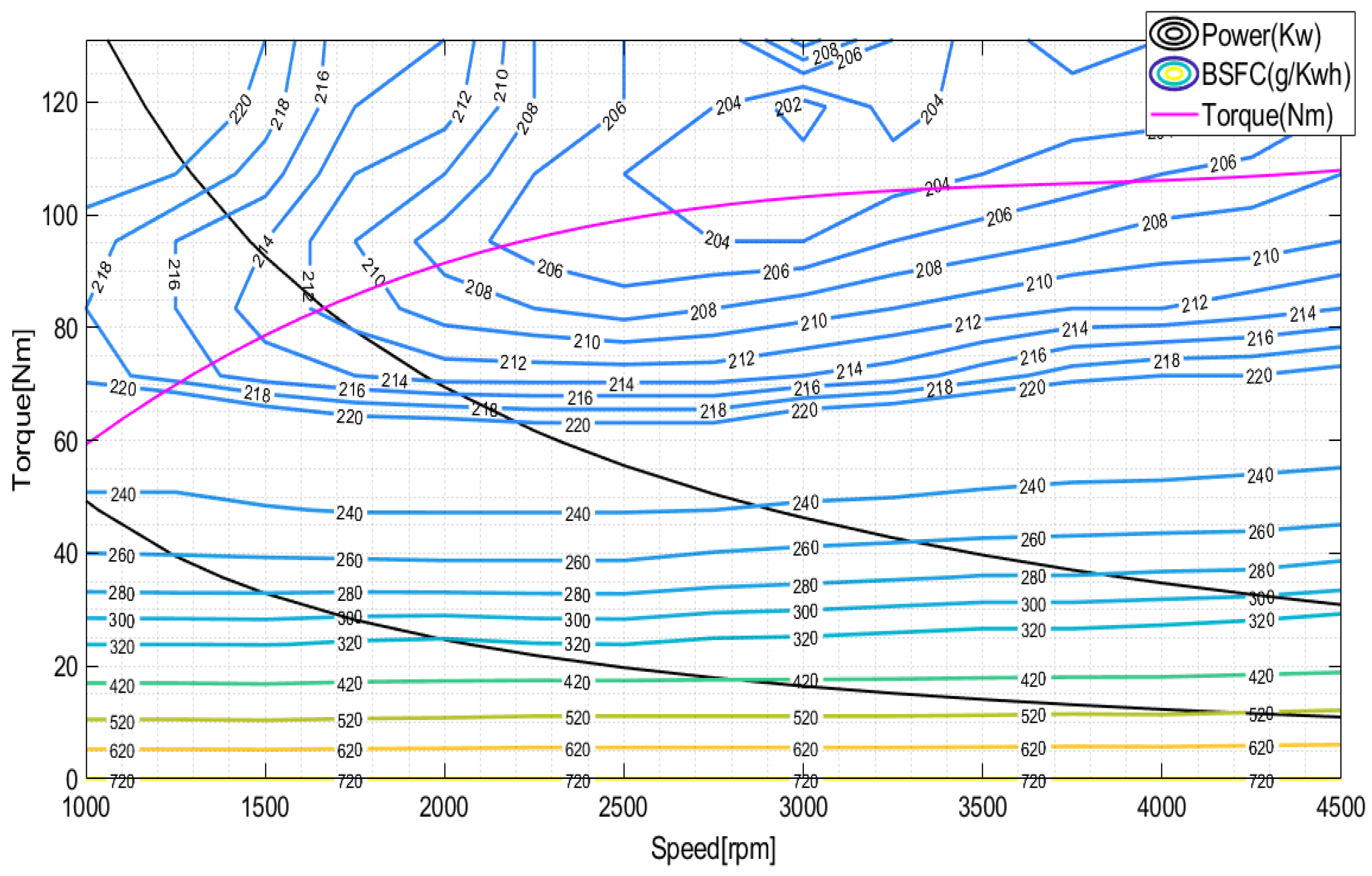
2.1. Powertrain Model

Serial–parallel HEVs distribute power using planetary gears. According to the mechanical connections between the gears, there are the following relations:

$$\left\{\begin{array}{c}(R_r+R_s){\omega }_c=R_r{\omega }_r+R_s{\omega }_s\hfill \\ T_r=\frac{R_r}{R_s+R_r}{T}_c,T_s=\frac{R_s}{R_s+R_r}{T}_c\hfill \end{array}\right.$$

(1)

where R, $\omega$ and T denote the radius, speed and torque of the gears, respectively. s, c, and r in the subscript represent the sun gear, carrier gear, and ring gear, respectively.

The dynamic with respect to the rotational speeds of generator, engine and motor can be obtained from Newton’s laws:

$$\left\{\begin{array}{c}{J}_g{\dot{\omega }}_g=T_s+T_g\hfill \\ J_e{\dot{\omega }}_e=T_e-T_c\hfill \\ J_m{\dot{\omega }}_m=T_m+T_r-\frac{T_{trac}}{g_f}\hfill \end{array}\right.$$

(2)

where J denotes the inertia. g, e, and m in the subscript represent generator, engine, and motor, respectively. $T_{trac}$ denotes the torque on the axle of the differential gear, and $g_f$ denotes the final gear ratio.

Assuming that the connecting shafts are rigid, the following speed relationships hold:

$${\omega }_c={\omega }_e,{\omega }_r={\omega }_m,{\omega }_s={\omega }_g,{\omega }_m=\frac{g_f}{R_{tire}}v$$

(3)

The dynamics of the vehicle velocity is modeled as:

$$M\dot{v}=\frac{{\eta }_f{T}_{trac}-T_{br}}{R_{tire}}-Mg({\mu }_{r}cos\theta +sin\theta )-\frac{1}{2}\rho A{C}_d{v}^2$$

(4)

where M and g denote the vehicle mass and the gravity acceleration, respectively. $T_{br}$ is the friction brake torque. ${\eta }_f$ is the transmission efficiency of differential gear; ${\mu }_r$ is the coefficient of rolling resistance; $\rho$ is air density; A is frontal area of vehicle; $C_d$ is drag coefficient; and $\theta$ is road angle. $R_{tire}$ is the tire radius. v is the vehicle velocity.

Fuel consumption is one term of the cost function, which is measured by the fuel mass flow rate ${\dot{m}}_f$ and is a function about engine torque and engine speed:

$${\dot{m}}_f=BSFC({\omega }_e,T_e)·T_e·{\omega }_e·{10}^{-3}·∆t/3600$$

(5)

where $∆t$ is sample time. $BSFC$ is brake specific fuel consumption, which can usually be described by a mapping of engine torque and engine speed. For example, the $BSFC$ diagram of a gasoline engine is shown in Figure 2 [14].

2.2. Battery Model

In the driving process, the battery state of charge ($SOC$) of the non-plug-in HEV needs to maintain near the initial value, and the final value is equal to its initial value. Capturing energy from braking charges the battery, and the electricity converted from the excess engine power also charges the battery. Like fuel consumption, electricity consumption is calculated by the instantaneous rate of change in the battery’s internal energy:

$$P_{elec}=U_{oc}·I_{batt}=-U_{oc}·Q_{batt}·\dot{S}OC$$

(6)

where $U_{oc}$, $I_{batt}$ and $Q_{batt}$ are battery open circuit voltage, current and maximum charge capacity, respectively. The instantaneous change rate of $SOC$ can be expressed as:

$$\dot{SOC}=\frac{-U_{oc}-\sqrt{U_{oc}^2-4R_b{P}_{batt}}}{2Q_{batt}{R}_b}$$

(7)

where $R_b$ is battery resistance, $P_{batt}$ is battery power. Both $U_{oc}$ and $R_b$ can be fitted as functions of $SOC$. The following relationship can be found:

$$P_{batt}={\eta }_m^{k_m}{T}_m{\omega }_m+{\eta }_g^{k_g}{T}_g{\omega }_g$$

(8)

where ${\eta }_m$ and ${\eta }_g$ denote the efficiency of motor and generator, respectively, and $k_m$, $k_g$ can be given by:

$$k_i=-1,\mathrm{dischraging};\mathrm{or}1,\mathrm{charging},i=m,g$$

(9)

2.3. Energy Management Optimization Problem

Energy management optimization control for the HEV is to ensure the minimization of the energy consumption during the whole journey while normal drivability of the vehicle. The energy consumption of HEV mainly includes fuel consumption and electric energy consumption, so the optimization goal is to minimize the equivalent fuel consumption. Accordingly, the optimization problem is formulated as follows.

To find the optimal control policy $u^{*}\left(t\right)$ such that:

$$J^{*}\left(t\right)=\underset{u}{min}\left\{J\left(t\right)=\sum _{i=t}^{t_{end}-1}{\gamma }^{i-t}·Q(x\left(i\right),u\left(i\right),i)\right\},t\in [t_0,t_{end}-1]$$

(10)

subject to the dynamic constraint condition

$$\left\{\begin{array}{c}SOC(t+1)=SOC\left(t\right)+∆t·\frac{-U_{oc}-\sqrt{U_{oc}^2-4R_b({\eta }_m^{k_m}{T}_m{\omega }_m+{\eta }_g^{k_g}{T}_g{\omega }_g)}}{2Q_{batt}{R}_b}\hfill \\ v(t+1)=\frac{∆t({\eta }_f{T}_{trac}-T_{br})}{M·R_{tire}}-g({\mu }_{r}cos\theta +sin\theta )·∆t-\frac{1}{2M}\rho A{C}_d{v}^2·∆t+v\left(t\right)\hfill \end{array}\right.$$

(11)

and the physical constraint conditions

$$\left\{\begin{array}{c}SO{C}_{min}\le SOC\le SO{C}_{max}\hfill \\ {\omega }_{e\_min}\le {\omega }_e\le {\omega }_{e\_max}\hfill \\ {\omega }_{m\_min}\le {\omega }_m\le {\omega }_{m\_max}\hfill \\ {\omega }_{g\_min}\le {\omega }_g\le {\omega }_{g\_max}\hfill \\ T_{e\_min}\left({\omega }_e\right)\le T_e\le T_{e\_max}\left({\omega }_e\right)\hfill \\ T_{m\_min}\left({\omega }_m\right)\le T_m\le T_{m\_max}\left({\omega }_m\right)\hfill \\ T_{g\_min}\left({\omega }_g\right)\le T_g\le T_{g\_max}\left({\omega }_g\right)\hfill \end{array}\right.$$

(12)

where $0<\gamma \le 1$ is the discount factor, $\lambda$ is the weight factor, $t_{end}$ is the total driving time. The state variable $x={\left[vSOC\right]}^T$ and the control input $u={\left[T_m{\omega }_g\right]}^T$. The instantaneous energy consumption Q is described as:

$$Q\left(t\right)=BSFC·T_e·{\omega }_e·∆t\times {10}^{-3}/3600+\lambda ·P_{elec}·∆t·3.6\times {10}^{-3}$$

(13)

with

$$\begin{array}{c}{P}_{elec}=\frac{U_{oc}^2-U_{oc}\sqrt{U_{oc}^2-4R_b{P}_{batt}({\omega }_g,T_m,v)}}{2R_b},\hfill \\ P_{batt}({\omega }_g,T_m,v)={\eta }_m^{k_m}{T}_m·\frac{g_f}{R_{tire}}v+{\eta }_g^{k_g}\left[P_{dem}-T_m·\frac{g_f}{R_{tire}}v-T_e(\frac{R_s}{R_r+R_s}{\omega }_g+\frac{R_r}{R_r+R_s}\frac{g_f}{R_{tire}}v)\right].\hfill \end{array}$$

(14)

As a consequence, the optimal control $u^{*}\left(t\right)$ is determined by solving the minimum of $J\left(t\right)$.

$$\begin{array}{c}{u}^{*}\left(t\right)=arg\underset{u\left(t\right)}{lim}\{J\left(t\right)=\sum _{i=t}^{t_{end}-1}{\gamma }^{i-t}·Q\left(i\right)\}\hfill \\ =arg\underset{u\left(t\right)}{lim}\{J\left(t\right)=Q\left(t\right)+\gamma ·J^{*}(t+1)\}\hfill \\ =arg\underset{u\left(t\right)}{lim}\{J\left(t\right)=Q\left(t\right)+\gamma ·Q(t+1)+{\gamma }^2·J^{*}(t+2)\}\hfill \\ =\dots \hfill \\ =\{u^{*}\left(t\right),\dots ,u^{*}(t_{end}-1)\}\hfill \end{array}$$

(15)

According to Bellman’s equation, it can be known that if $J^{*}(t+1)$ in the above equation is known at time t, the value of $u^{*}\left(t\right)$ can be calculated by the DP method. $J^{*}(t+1)$ represents the minimum energy consumption from the time $t+1$ to the final driving time $t_{end}$ of the vehicle. However, to obtain $J^{*}(t+1)$, it is necessary to know the driving information of the time $t+1$ to the final driving time $t_{end}$ in advance. DP is difficult to achieve energy management control under unknown driving conditions. In addition, DP utilizes the backward iterative algorithm to obtain the optimal solution, which requires a large amount of calculation and takes a long time.

ADP is developed based on DP, and its idea is consistent with the Actor–Critic framework in RL. The NN is used to replace the action model and critic functions. The critic network outputs the approximate value $\widehat{J}(t+1)$ of $J^{*}(t+1)$ through inputting state variables, and the action network outputs the approximate value $\widehat{u}\left(t\right)$ of $u^{*}\left(t\right)$. In this process of obtaining $J^{*}(t+1)$, the ADP method updates the network weight by calculating the error value and optimizes the parameters of the nonlinear function continuously to render $\widehat{J}(t+1)$ gradually to approach $J^{*}(t+1)$. Based on this, the output $\widehat{u}\left(t\right)$ of the action network can be seen as $u^{*}\left(t\right)$, which is just the optimal solution in the DP. This control strategy does not require the driving information in advance and allows energy management of the HEV to be online and in real-time. Therefore, this paper designs a real-time EMS of HEV using the DHP method, detailed in the next section.

3. Design of DHP-Based Real-Time EMS

The diagram structure of the designed DHP-based real-time energy management control system of the HEV is shown in Figure 3.

The DHP-based real-time EMS is comprised of the speed prediction for obtaining the power demand of the vehicle and the DHP algorithm for the power distribution. The speed prediction model is established by the BPNN offline trained by history traffic data. A PID-type driver model obtains the power demand (traction torque of the vehicle wheel). The DHP algorithm structure includes an action network (AN), a dynamic model, and two critic networks, CN1 and CN2. AN describes the mapping between the state $x\left(t\right)$ and the approximate $\widehat{u}\left(t\right)$, CN1 describes the mapping between the state $x\left(t\right)$ and the derivative of performance indicator J to state x, $\frac{\partial \widehat{J}\left(t\right)}{\partial x\left(t\right)}$, and CN2 similarly describes the mapping between the state $x(t+1)$ and $\frac{\partial \widehat{J}(t+1)}{\partial x(t+1)}$. The dynamic model represents the HEV model by function relation, which calculates the state value $x(t+1)$ at the next moment by inputting the approximate value $\widehat{u}\left(t\right)$ of the control value.

In the DHP algorithm structure, the error between $\frac{\partial \widehat{J}\left(t\right)}{\partial x\left(t\right)}$ and $\frac{\partial Q\left(t\right)}{\partial x\left(t\right)}+\frac{\partial \gamma \widehat{J}(t+1)}{\partial x(t+1)}$ is used to train CNs parameters. This process is executed in a cycle when the HEV is running, and after training the network continuously, $\frac{\partial \widehat{J}\left(t\right)}{\partial x\left(t\right)}=\frac{\partial Q\left(t\right)}{\partial x\left(t\right)}+\frac{\partial \gamma \widehat{J}(t+1)}{\partial x(t+1)}$ is obtained. At this time, the output $\widehat{u}\left(t\right)$ of AN can be regarded as the optimal control value $u^{*}\left(t\right)$, and the output $\frac{\partial \widehat{J}\left(t\right)}{\partial x\left(t\right)}$ of CN1 can be regarded as the optimal co-state $\frac{\partial J^{*}\left(t\right)}{\partial x\left(t\right)}$. Where $\widehat{J}\left(t\right)$ can be regarded as the optimal cost function $J^{*}\left(t\right)$. It is worth noting that CN1 and CN2 update weight parameters synchronously, and the two networks are the same. In this control process, the idea and process of this strategy of constantly adjusting network parameters of AN and CN is similar to the RL strategy.

BPNN possesses strong nonlinear fitting and self-learning abilities. Based on this characteristic, BPNN is selected to construct the prediction model, AN, and CN. The detailed design of the speed prediction model, AN, and CN will be introduced below.

3.1. Speed Prediction Model

The speed prediction model adopts the BPNN structure [41] shown in Figure 4.

The objective function of the network can be expressed as

$$\begin{array}{c}\mathbf{Y}=F\left(\mathbf{X}\right)\hfill \\ \mathbf{X}=[v_{t-∆H},\dots ,v_{t-1},v_t]\hfill \\ \mathbf{Y}=[v_{t+1},v_{t+2},\dots ,v_{t+∆P}]\hfill \end{array}$$

(16)

where F represents the objective function of neural network training, $∆P$ and $∆H$ are the predict horizon and input horizon, respectively.

Many historical vehicle speeds were used to train the BPNN offline, and then the trained network was used to predict the HEV speed online. When the BPNN model is used to predict the speed online, the current speed and the speed of the several previous instants, namely the historical speed sequence, are used as inputs into the speed prediction model to obtain the speed of the prediction sequence. The training set of the speed prediction model is from the actual commuting speed data collected on conventional routes in urban traffic, which is provided by JSAE-SICE benchmark problem 2, see [42].

In the application of speed prediction in this paper, only the speed at the next instant needs to predict, so the output sets as $v_{t+1}$.

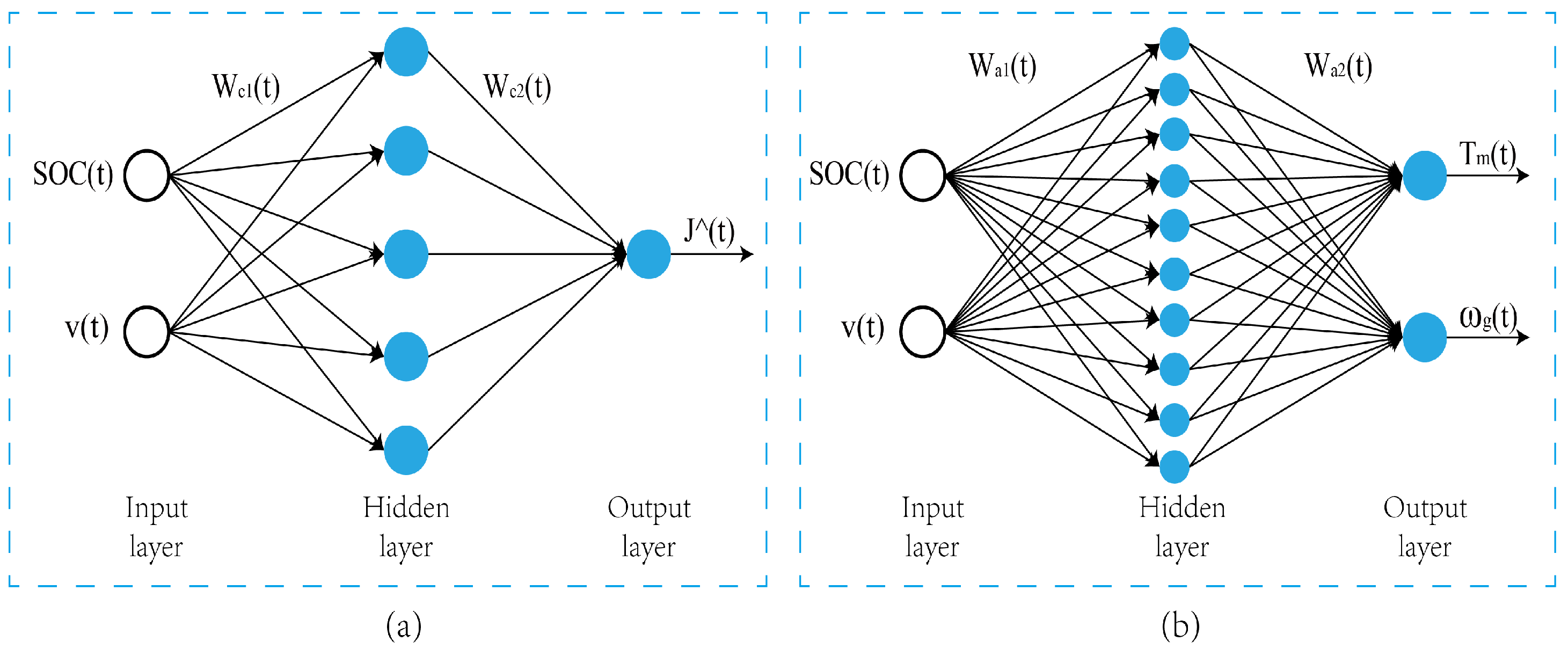
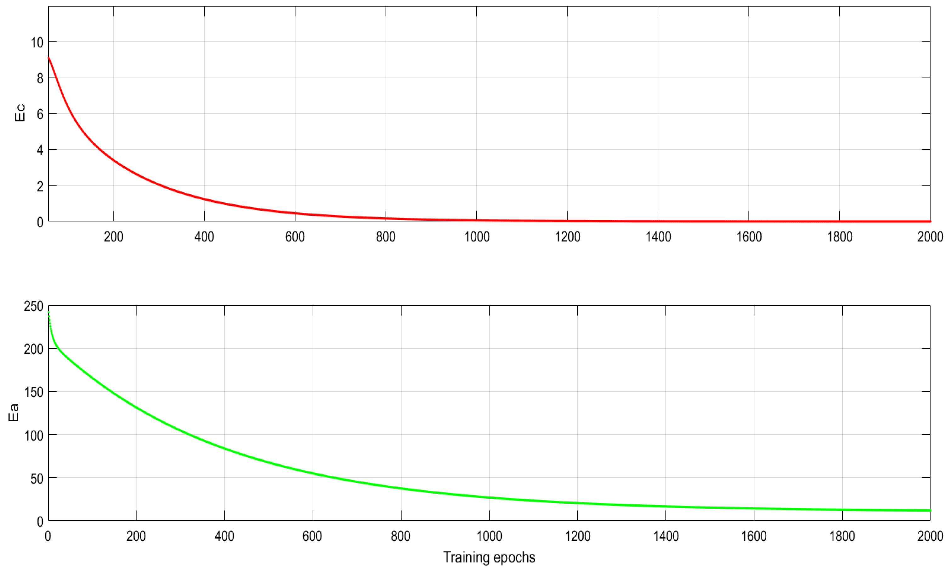
3.2. Design of Critic Network

Figure 5a shows the BPNN structure of CN. Where the input layer has two nodes of two-state values of HEV, the hidden layer number of the network is set as one with five nodes, and the output layer has one node of the output value $\frac{\partial \widehat{J}\left(t\right)}{\partial x\left(t\right)}$. The transfer functions of the hidden and output layers are the tansig and purelin functions, respectively. Thus, the nonlinear function of CN can be described as:

$$\left\{\begin{array}{c}{\mathbf{c}}_1\left(t\right)=x\left(t\right)\times {\mathbf{W}}_{c1}\left(t\right)\hfill \\ {\mathbf{c}}_2\left(t\right)=\frac{1-e^{-{\mathbf{c}}_1\left(t\right)}}{1+e^{-{\mathbf{c}}_1\left(t\right)}}\hfill \\ \frac{\partial \widehat{J}\left(t\right)}{\partial x\left(t\right)}={\mathbf{c}}_2\left(t\right)\times {\mathbf{W}}_{c2}\left(t\right)\hfill \end{array}\right.$$

(17)

where $x\left(t\right)=[v,SOC]$, ${\mathbf{c}}_1$ and ${\mathbf{c}}_2$ are the inputs and outputs of hidden layer nodes. ${\mathbf{W}}_{c1}$ and ${\mathbf{W}}_{c2}$ represent the weight matrices from the input layer to the hidden layer and from the hidden layer to the output layer, respectively, with the structure as follows:

$${\mathbf{W}}_{c1}=\left[\begin{array}{ccccc}{W}_{11}\left(t\right)& W_{12}\left(t\right)& W_{13}\left(t\right)& W_{14}\left(t\right)& W_{15}\left(t\right)\\ W_{21}\left(t\right)& W_{22}\left(t\right)& W_{23}\left(t\right)& W_{24}\left(t\right)& W_{25}\left(t\right)\end{array}\right]$$

(18)

$${\mathbf{W}}_{c2}^T=\left[\begin{array}{ccccc}{W}_{11}\left(t\right)& W_{21}\left(t\right)& W_{31}\left(t\right)& W_{41}\left(t\right)& W_{51}\left(t\right)\\ W_{12}\left(t\right)& W_{22}\left(t\right)& W_{32}\left(t\right)& W_{42}\left(t\right)& W_{52}\left(t\right)\end{array}\right]$$

(19)

The purpose of training CN is to keep the actual value $\frac{\partial Q\left(t\right)}{\partial x\left(t\right)}+\frac{\partial \gamma \widehat{J}(t+1)}{\partial x(t+1)}$ approaching the target value $\frac{\partial \widehat{J}\left(t\right)}{\partial x\left(t\right)}$. Therefore, the error function of CN can be defined as the difference between the target value and the actual value, i.e.,

$$e_c\left(t\right)=\frac{\partial \widehat{J}\left(t\right)}{\partial x\left(t\right)}-\frac{\partial Q\left(t\right)}{\partial x\left(t\right)}-\gamma ·\frac{\partial J^{*}(t+1)}{\partial x(t+1)}$$

(20)

To make the value of the error function converge to 0, let:

$$E_c\left(t\right)=\frac{1}{2}{e}_c^2\left(t\right)\le {\epsilon }_c$$

(21)

where ${\epsilon }_c$ is a default error value very close to 0, $E_c$ is used to train network weights. In order to achieve this goal, we chose the gradient descent algorithm to train ${\mathbf{W}}_{c1}$ and ${\mathbf{W}}_{c2}$. If let $\dot{J}\left(t\right)=\frac{\partial \widehat{J}\left(t\right)}{\partial x\left(t\right)}$, the update of ${\mathbf{W}}_{c1}$ and ${\mathbf{W}}_{c2}$ are calculated as follows:

$$\left\{\begin{array}{c}∆{\mathbf{W}}_{c1}\left(t\right)={\eta }_c·[-\frac{\partial E_c\left(t\right)}{\partial {\mathbf{W}}_{c1}\left(t\right)}]\hfill \\ \frac{\partial E_c\left(t\right)}{\partial {\mathbf{W}}_{c1}\left(t\right)}=\frac{\partial E_c\left(t\right)}{\partial \dot{J}\left(t\right)}·\frac{\partial \dot{J}\left(t\right)}{\partial {\mathbf{c}}_2\left(t\right)}·\frac{\partial {\mathbf{c}}_2\left(t\right)}{\partial {\mathbf{c}}_1\left(t\right)}·\frac{\partial {\mathbf{c}}_1\left(t\right)}{\partial {\mathbf{W}}_{c1}\left(t\right)}\hfill \\ {\mathbf{W}}_{c1}(t+1)={\mathbf{W}}_{c1}\left(t\right)+∆{\mathbf{W}}_{c1}\left(t\right)\hfill \end{array}\right.$$

(22)

$$\left\{\begin{array}{c}∆{\mathbf{W}}_{c2}\left(t\right)={\eta }_c·[-\frac{\partial E_c\left(t\right)}{\partial {\mathbf{W}}_{c2}\left(t\right)}]\hfill \\ \frac{\partial E_c\left(t\right)}{\partial {\mathbf{W}}_{c2}\left(t\right)}=\frac{\partial E_c\left(t\right)}{\partial \dot{J}\left(t\right)}·\frac{\partial \dot{J}\left(t\right)}{\partial {\mathbf{W}}_{c2}\left(t\right)}\hfill \\ {\mathbf{W}}_{c2}(t+1)={\mathbf{W}}_{c2}\left(t\right)+∆{\mathbf{W}}_{c2}\left(t\right)\hfill \end{array}\right.$$

(23)

where $0<{\eta }_c\le 1$ is the learning factor.

3.3. Design of Actor Network

Figure 5b shows the structure of AN. In the same way, we use BPNN to design AN. The hidden layer number of AN is one in which the input layer has two nodes of the two-state of HEV, the hidden layer has ten nodes, and the output layer has two nodes of the control values $\widehat{u}\left(t\right)$. Experiments show that the network has the best effect when the number of hidden layer nodes is 10. The transfer functions of the hidden layer and output layer are consistent with CN. Thus, the nonlinear function of AN can be described as:

$$\left\{\begin{array}{c}{\mathbf{a}}_1\left(t\right)=x\left(t\right)\times {\mathbf{W}}_{a1}\left(t\right)\hfill \\ {\mathbf{a}}_2\left(t\right)=\frac{1-e^{-{\mathbf{a}}_1\left(t\right)}}{1+e^{-{\mathbf{a}}_1\left(t\right)}}\hfill \\ \widehat{u}\left(t\right)={\mathbf{a}}_2\left(t\right)\times {\mathbf{W}}_{a2}\left(t\right)\hfill \end{array}\right.$$

(24)

where $\widehat{u}\left(t\right)=[T_m,{\omega }_g]$, ${\mathbf{a}}_1$ and ${\mathbf{a}}_2$ are the inputs and outputs of hidden layer nodes. ${\mathbf{W}}_{a1}$ and ${\mathbf{W}}_{a2}$ represent the weight matrices from input layer to hidden layer and from hidden layer to output layer, respectively.

According to the principle of optimality, the optimal control should satisfy the necessary condition of first-order differential, i.e.,

$$\frac{\partial J^{*}\left(t\right)}{\partial u\left(t\right)}=\frac{\partial Q\left(t\right)}{\partial u\left(t\right)}+\frac{\partial \gamma ·J^{*}(t+1)}{\partial u\left(t\right)}$$

(25)

so, the optimal control can be obtained:

$$u^{*}\left(t\right)=arg\underset{u\left(t\right)}{lim}\left\{\left|\frac{\partial J^{*}\left(t\right)}{\partial u\left(t\right)}-\frac{\partial Q\left(t\right)}{\partial u\left(t\right)}-\frac{\partial \gamma ·J^{*}(t+1)}{\partial x(t+1)}·\frac{\partial x(t+1)}{\partial u\left(t\right)}\right|\right\}$$

(26)

where $\frac{\partial \gamma ·J^{*}(t+1)}{\partial x(t+1)}$ is the optimal co-state, which can be obtained directly from the output of CN2, and $\frac{\partial x(t+1)}{\partial u\left(t\right)}$ can be obtained from the input–output relation of the dynamic model.

In this paper, we adopt the optimization method to find the optimal control value. In the process of network update iteratively, i is set as the number of iterations. For every $\frac{\partial \widehat{J}\left(i\right)}{\partial x\left(i\right)}$ and $\frac{\partial \widehat{J}(i+1)}{\partial x(i+1)}$ of CN at a certain time, search for $u^{*}\left(i\right)$ until getting the optimal control at that time. Therefore, the update process for ${\mathbf{W}}_{a1}$ and ${\mathbf{W}}_{a2}$ are as follows:

$$E_a\left(t\right)=\frac{1}{2}{[u^{*}\left(t\right)-\widehat{u}\left(t\right)]}^2\le {\epsilon }_a$$

(27)

$$\left\{\begin{array}{c}∆{\mathbf{W}}_{a1}\left(t\right)={\eta }_a·\left[-\frac{\partial E_a\left(t\right)}{\partial {\mathbf{W}}_{a1}\left(t\right)}\right]\hfill \\ {\mathbf{W}}_{a1}(t+1)={\mathbf{W}}_{a1}\left(t\right)+∆{\mathbf{W}}_{a1}\left(t\right)\hfill \end{array}\right.$$

(28)

$$\left\{\begin{array}{c}∆{\mathbf{W}}_{a2}\left(t\right)={\eta }_a·\left[-\frac{\partial E_a\left(t\right)}{\partial {\mathbf{W}}_{a2}\left(t\right)}\right]\hfill \\ {\mathbf{W}}_{a2}(t+1)={\mathbf{W}}_{a2}\left(t\right)+∆{\mathbf{W}}_{a2}\left(t\right)\hfill \end{array}\right.$$

(29)

where $0<{\eta }_a\le 1$ is the learning factor. ${\epsilon }_a$ is a predetermined error value very close to 0.

3.4. DHP-Based Real-Time EMS

The specific implementation process of the DHP-based EMS algorithm framework in Figure 3 is as follows:

(1) Initialize HEV parameters and initialize AN and CNs parameters.

(2) Input the next time speed $v(t+1)$ predicted by the speed prediction model and the current time speed $v\left(t\right)$ into the PID controller, and calculate the demand torque $T_{trac}\left(t\right)$ at the current moment;

(3) According to the current state $x\left(t\right)=\left[v\right(t),SOC(t\left)\right]$ of HEV, CN1 calculates the co-state $\frac{\partial \widehat{J}\left(t\right)}{\partial x\left(t\right)}$ by (17), and AN calculates the control $\widehat{u}\left(t\right)=[T_m\left(t\right),{\omega }_g\left(t\right)]$ by (24);

(4) According to the control policy obtained in the previous step, the dynamic model calculates the state $x(t+1)=\left[v\right(t+1),SOC(t+1\left)\right]$ at the next moment through (11), and calculates the instantaneous energy consumption $Q\left(t\right)$ by (13).

(5) According to the state $x(t+1)$ at the next moment, CN2 calculates $\frac{\partial \widehat{J}(t+1)}{\partial x(t+1)}$ by (17), then calculates $E_c\left(t\right)$ and $u^{*}\left(t\right)$ by (21) and (26), and calculates $E_a\left(t\right)$ by (27).

(6) Determine whether $E_c\left(t\right)$ is less than or equal to ${\epsilon }_c$, and whether $E_a\left(t\right)$ is less than or equal to ${\epsilon }_a$. When any of the conditions cannot be met, the parameters of AN and CN should be updated. Formulas (22) and (23) are used to update weights ${\mathbf{W}}_{c1}$ and ${\mathbf{W}}_{c2}$ of CN, and Formulas (28) and (29) are used to update weights ${\mathbf{W}}_{a1}$ and ${\mathbf{W}}_{a2}$ of AN. Then step (3) to step (6) are repeated until both conditions are met, when the next step is carried out.

(7) Provide the optimal control calculated in the current moment to the HEV, then go back to step (2) and continue to calculate the control policy for the next moment until the HEV completes driving.

The detailed algorithm flow of the DHP-based EMS is illustrated in Algorithm 1. Below is the description of the DHP algorithm.

Algorithm 1: Online learning algorithm of HEV with DHP.

Parameters initialization       State variable: SOC, v; Discount factor: $\gamma$;       Weights in CN: ${\mathbf{W}}_{c1}$, ${\mathbf{W}}_{c2}$; Weights in AN: ${\mathbf{W}}_{a1}$, ${\mathbf{W}}_{a2}$;       Learning factor of CN and AN: ${\eta }_c$, ${\eta }_a$; error value: ${\epsilon }_c$, ${\epsilon }_a$; for $i=1:t_{end}$     Speed prediction and demand torque determination       Getting the current speed $v\left(i\right)$ from HEV;       Running the speed prediction model to abtain $v(i+1)$;       Using PID controller to get $T_{trac}\left(i\right)$;     Estimating $\widehat{u}\left(i\right)$ and $\frac{\partial \widehat{J}\left(i\right)}{\partial x\left(i\right)}$       CN1: $\frac{\partial \widehat{J}\left(i\right)}{\partial x\left(i\right)}=f(SOC\left(i\right),v\left(i\right),{\mathbf{W}}_{c1}\left(i\right),{\mathbf{W}}_{c2}\left(i\right))$;       AN: $\widehat{u}\left(i\right)=f(SOC\left(i\right),v\left(i\right),{\mathbf{W}}_{a1}\left(i\right),{\mathbf{W}}_{a2}\left(i\right))$;       $\widehat{u}\left(i\right)=[T_m\left(i\right),{\omega }_g\left(i\right)]$;     Calculating $x(i+1)$ and $Q\left(i\right)$       $x(i+1)=x\left(i\right)+∆x\left(i\right)$;       $Q\left(i\right)=(BSFC\left(i\right)·T_e\left(i\right)·{\omega }_e\left(i\right)/3600+\lambda ·P_{elec}\left(i\right)·3.6)\times {10}^{-3}$;     Calculating $E_c\left(i\right)$ and $E_a\left(i\right)$       CN2: $\frac{\partial \widehat{J}(i+1)}{\partial x(i+1)}=f(SOC(i+1),v(i+1),{\mathbf{W}}_{c1}\left(i\right),{\mathbf{W}}_{c2}\left(i\right))$;       $E_c\left(i\right)=\frac{1}{2}{[\frac{\partial \widehat{J}\left(i\right)}{\partial x\left(i\right)}-\frac{\partial Q\left(i\right)}{\partial x\left(i\right)}-\gamma ·\frac{\partial J^{*}(i+1)}{\partial x(i+1)}]}^2$;       $u^{*}\left(i\right)=arg{lim}_{u\left(i\right)}\left\{\right|\frac{\partial J^{*}\left(i\right)}{\partial u\left(i\right)}-\frac{\partial Q\left(i\right)}{\partial u\left(i\right)}-\frac{\partial \gamma ·J^{*}(i+1)}{\partial x(i+1)}·\frac{\partial x(i+1)}{\partial u\left(i\right)}\left|\right\}$;       $E_a\left(i\right)=\frac{1}{2}{[u^{*}\left(i\right)-\widehat{u}\left(i\right)]}^2$;     Optimal control judgement     while $E_c\left(i\right)>{\epsilon }_c$ and $E_a\left(i\right)>{\epsilon }_a$       Weights update         ${\mathbf{W}}_{c1}\left(i\right)={\mathbf{W}}_{c1}\left(i\right)+∆{\mathbf{W}}_{c1}\left(i\right)$; ${\mathbf{W}}_{c2}\left(i\right)={\mathbf{W}}_{c2}\left(i\right)+∆{\mathbf{W}}_{c2}\left(i\right)$;         ${\mathbf{W}}_{a1}\left(i\right)={\mathbf{W}}_{a1}\left(i\right)+∆{\mathbf{W}}_{a1}\left(i\right)$; ${\mathbf{W}}_{a2}\left(i\right)={\mathbf{W}}_{a2}\left(i\right)+∆{\mathbf{W}}_{a2}\left(i\right)$;       Estimating $\widehat{u}\left(i\right)$ and $\frac{\partial \widehat{J}\left(i\right)}{\partial x\left(i\right)}$         CN1: $\frac{\partial \widehat{J}\left(i\right)}{\partial x\left(i\right)}=f(SOC\left(i\right),v\left(i\right),{\mathbf{W}}_{c1}\left(i\right),{\mathbf{W}}_{c2}\left(i\right))$;         AN: $\widehat{u}\left(i\right)=f(SOC\left(i\right),v\left(i\right),{\mathbf{W}}_{a1}\left(i\right),{\mathbf{W}}_{a2}\left(i\right))$;         $\widehat{u}\left(i\right)=[T_m\left(i\right),{\omega }_g\left(i\right)]$;       Calculating $x(i+1)$ and $Q\left(i\right)$         $x(i+1)=x\left(i\right)+∆x\left(i\right)$;         $Q\left(i\right)=(BSFC\left(i\right)·T_e\left(i\right)·{\omega }_e\left(i\right)/3600+\lambda ·P_{elec}\left(i\right)·3.6)\times {10}^{-3}$;       Calculating $E_c\left(i\right)$ and $E_a\left(i\right)$         CN2: $\frac{\partial \widehat{J}(i+1)}{\partial x(i+1)}=f(SOC(i+1),v(i+1),{\mathbf{W}}_{c1}\left(i\right),{\mathbf{W}}_{c2}\left(i\right))$;         $E_c\left(i\right)=\frac{1}{2}{[\frac{\partial \widehat{J}\left(i\right)}{\partial x\left(i\right)}-\frac{\partial Q\left(i\right)}{\partial x\left(i\right)}-\gamma ·\frac{\partial J^{*}(i+1)}{\partial x(i+1)}]}^2$;         $u^{*}\left(i\right)=arg{lim}_{u\left(i\right)}\left\{\right|\frac{\partial J^{*}\left(i\right)}{\partial u\left(i\right)}-\frac{\partial Q\left(i\right)}{\partial u\left(i\right)}-\frac{\partial \gamma ·J^{*}(i+1)}{\partial x(i+1)}·\frac{\partial x(i+1)}{\partial u\left(i\right)}\left|\right\}$;         $E_a\left(i\right)=\frac{1}{2}{[u^{*}\left(i\right)-\widehat{u}\left(i\right)]}^2$;     end while       $u^{*}\left(i\right)=\widehat{u}\left(i\right)$    $u^{*}\left(i\right)\to HEV$   end for

4. Simulation Verification and Results Discussion

Firstly, the simulation demonstrates the effectiveness and advantages of the BPNN model in the DHP algorithm structure.

For the AN and CNs, the initial network weights are randomly set values, the learning rates are 0.01, the discount factor is 0.95, and the error value is 0.001. The number of network iterations is 2000. The initial value of SOC is 0.5.

Figure 6 shows the convergence curves of $E_c$ and $E_a$. In the process of continuous networks iteration and constant weights update, the value of $E_c$ approaches zero infinitely, and the value of $E_a$ approaches a constant. These show the effectiveness of network training. Figure 7 shows the convergence curve of $E_a$ in different hidden layer nodes of AN. It can be seen from the curve that as the number of nodes in the hidden layer increases, the convergence speed of $E_a$ accelerates, and the number of iterations when $E_a$ approaches a constant value also decreases. However, the increase in nodes in the hidden layer will lead to added training time, so the training time should also be considered when considering the convergence effect.

Table 2. The number of iterations and training time of different hidden layer nodes.

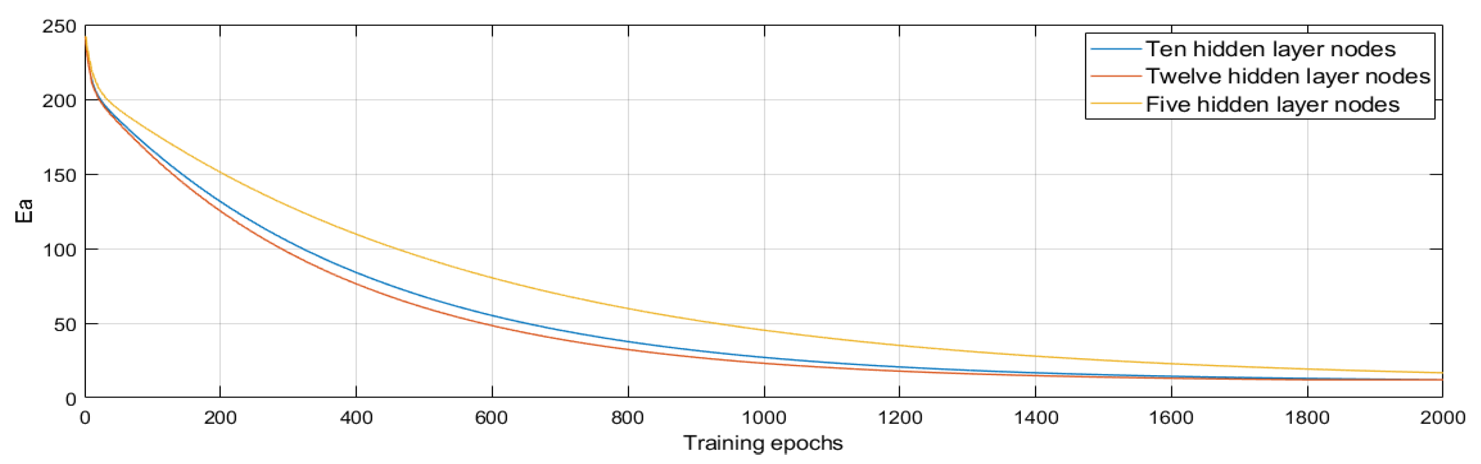
Hidden Layer Nodes	Iterations	Training Time (s)
5	2800	13,725
10	2000	12,680
12	1800	14,500

shows the number of iterations and training time required by the different number of hidden layer nodes, which means that when the number of hidden layer nodes of AN is 10, the training time and the convergence effect are appropriate. By adjusting network parameters, the training speed is faster. The results show that DHP has a higher algorithm accuracy than the HDP, and the increase in computational load does not significantly prolong the training time.

Table 3. The weight of the CN and AN.

${\mathbf{W}}_{c1}(2\times 5)$	3.819  4.204  4.274  −5.009  −4.597
	8.426  8.100  8.331  −8.080  −4.597
${\mathbf{W}}_{c2}^T(5\times 1)$	0.234   1.582  0.471   −1.693   0.520
${\mathbf{W}}_{a1}(2\times 10)$	0.168  0.881  −0.245  0.039  −0.387  −0.158  0.640  0.133  0.164  0.114
	0.975  0.358  −0.050  0.555    0.115  0.257  0.205  0.368  0.628  0.544
${\mathbf{W}}_{a2}^T(10\times 2)$	−0.384  0.004  0.486  0.250  −0.084  0.541  0.448  0.085  −0.035  0.037
	0.287  0.141  0.645  0.820   0.886  0.776  0.147  0.718     0.476  0.332

shows the weights of the final training of AN and CN, that is, the weight symbols and their corresponding matrix sequences.

Next, for an actual driving cycle, simulation comparisons with the HDP-based EMS and the RB-based EMS will be given to verify the effectiveness of the DHP-based real-time EMS for the fuel economy under the constraints of driving power demand and SOC. The simulation results of the speed tracking curve, the SOC fluctuation curve, and the equivalent fuel consumption of the three EMSs are shown in Figure 8. Meanwhile, Figure 9, Figure 10 and Figure 11 show the torque and speed curves of the engine, motor, and generator for these three strategies, respectively.

For clarity of comparison, the comparison results of the three EMSs are listed in

Table 4. Comparisons among DHP-based EMS, HDP-based EMS and RB-based EMS.

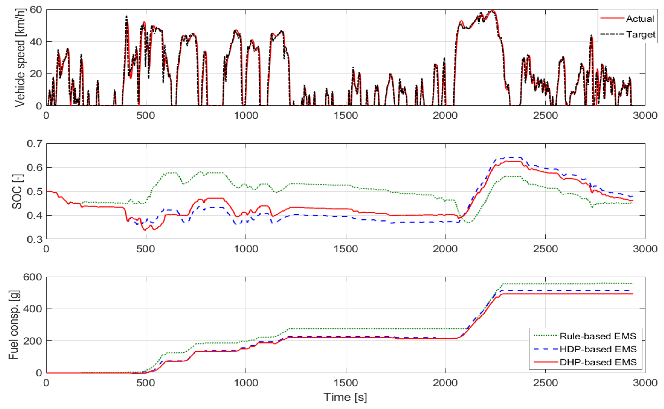
Algorithm	Final SOC	Equival. Fuel Consump. (g)	Reduction (%)
RB	0.452	557.8	−
HDP	0.479	514.9	7.69
DHP	0.462	492.9	11.63

. From Table 4, the simulation results show that with the difference in SOC final value of the three strategies being small, the equivalent fuel consumption of the DHP-based EMS is the least, which significantly improves the fuel economy.

The adaptability of the learning-based EMS to different driving conditions is then verified. In order to verify the adaptability of the DHP strategy, the DHP-based EMS is compared with other learning-based EMS in one different driving condition. Here, an energy management strategy based on a double deep Q-Network proposed in [43] is compared, in which the deep neural network is combined with Q-learning in reinforcement learning, having specific adaptability to complex and changeable working conditions. The simulation comparison result of the DHP-based EMS, the HDP-based EMS, and the DDQN-based EMS is shown in Figure 12. The comparisons of the three energy management strategies are also listed in

Table 5. Comparison of DHP-based EMS, HDP-based EMS and DDQN-based EMS.

Algorithm	Final SOC	Equival. Fuel Consump. (g)	Reduction (%)
DDQN	0.359	574.1	−
HDP	0.391	552.6	3.74
DHP	0.395	519.1	9.58

.

It can be seen from Figure 12 that the DHP-based EMS makes HEV achieve higher fuel economy under different driving conditions than the others. Specifically, the DHP-based EMS reduces the equivalent fuel consumption by 9.58% compared with the DDQN strategy, and by 6.06% compared with the HDP strategy. Moreover, in DHP-based EMS, the output of CN is co-state, which uses the performance index itself to approximate the optimal control, resulting in the network being able to estimate the solution closer to the optimal value using the co-state training network. When the trained DHP-based EMS is applied in different driving conditions, the network weights in the DHP algorithm will be slightly adjusted according to different driving conditions. The simulation results verify that the proposed DHP-based EMS can continuously learn based on the current driving information and has better adaptability to changeable driving conditions.

Finally, to further verify the adaptability of the proposed EMS to various driving conditions, the above three learning-based EMSs (DDQN, HDP, and DHP ) are simulated under the New European Driving Cycle (NEDC). Figure 13 shows the simulation results.

Table 6. Comparisons among the three learning-based EMSs in NEDC driving cycle.

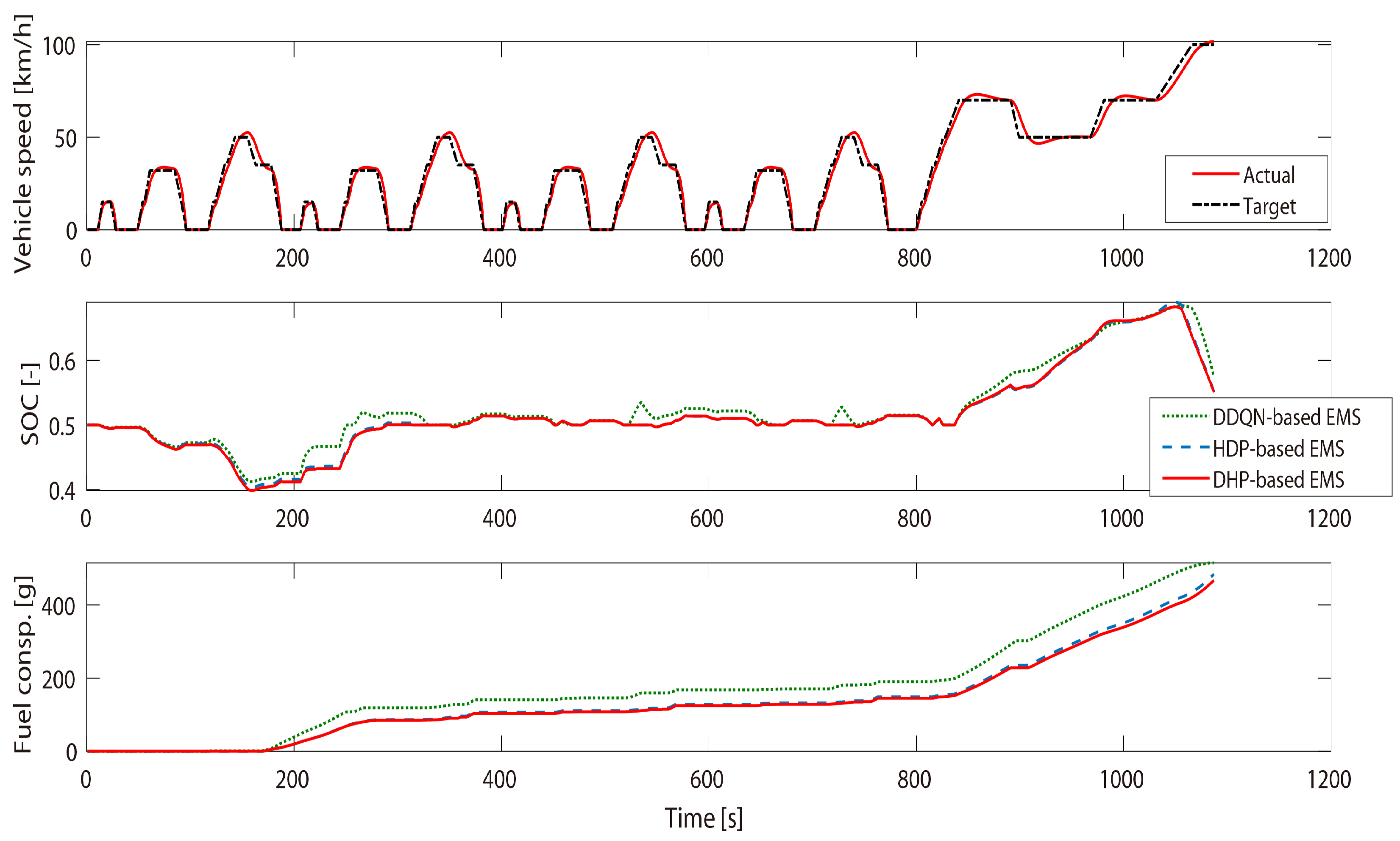
Algorithm	Final SOC	Equival. Fuel Consump. (g)	Reduction (%)
DDQN	0.574	515.0	−
HDP	0.552	488.3	5.18
DHP	0.551	480.5	6.70

lists the comparison results of the three strategies. They show that the EMS proposed in this paper has low equivalent fuel consumption when the final SOC values of the three strategies are almost the same. It further indicates that the EMS proposed in this paper has wide applicability.

5. Conclusions

This paper designed a DHP-based real-time EMS for HEVs. The EMS aims to achieve maximum energy saving for HEV even without prior driving information. The actor–critic thought in DHP effectively solves the problem of "dimensional disaster" of the traditional optimization algorithm DP. Without knowing all driving information in advance, the DHP can learn and adjust network parameters in real-time to optimize strategies. The proposed EMS was verified by simulation under various driving conditions, including actual and NEDC driving cycles. By analyzing the simulation results, the output torque of the proposed DHP-based EMS can effectively make the HEV track the desired speed, and the speed tracking accuracy can reach more than 95%. Compared with the HDP-based EMS, the accuracy of the DHP algorithm is indeed higher. On the premise of ensuring real-time performance, the DHP-based EMS can further reduce the equivalent fuel consumption of HEV compared with the two existing learning-based EMSs. For the actual driving cycle, the DHP-based EMS reduces the equivalent fuel consumption by 9.58% compared with the DDQN strategy and by 6.06% compared with the HDP strategy. In the NEDC driving cycle, the DHP-based EMS reduces the equivalent fuel consumption by 6.70% compared with the DDQN strategy, and by 1.60% compared with the HDP strategy. The results verify the effectiveness, fuel economy, and adaptability under different driving conditions of DHP-based EMS.

In addition, the states in EMS proposed in this paper are HEV speed v and SOC. A relatively single selection of state variables is not conducive to fitting the relationship between input and output of the network, and more iterations are needed to make the parameters converge. In future studies, we will design EMS by increasing the state input in the network so that the network can learn more quickly and make corresponding decisions, aiming to further improve the energy consumption optimization performance of the proposed online EMS.

References

- Salmasi, F.R. Control strategies for hybrid electric vehicles: Evolution, classification, comparison, and future trends. IEEE Trans. Veh. Technol. 2007, 56, 2393–2404. [Google Scholar] [CrossRef]
- Caiazzo, B.; Coppola, A.; Petrillo, A.; Santini, S. Distributed nonlinear model predictive control for connected autonomous electric vehicles platoon with distance-dependent air drag formulation. Energies 2021, 14, 5122. [Google Scholar] [CrossRef]
- Tran, D.D.; Vafaeipour, M.; Baghdadi, M.E.; Barrero, R.; Van Mierlo, J.; Hegazy, O. Thorough state-of-the-art analysis of electric and hybrid vehicle powertrains: Topologies and integrated energy management strategies. Renew. Sustain. Energy Rev. 2020, 119, 109596. [Google Scholar] [CrossRef]
- Lekshmi, S.; Lal Priya, P.S. Mathematical modeling of electric vehicles—A survey. Control Eng. Pract. 2019, 92, 104138. [Google Scholar]
- Enang, W.; Bannister, C. Modelling and control of hybrid electric vehicles (A comprehensive review). Renew. Sustain. Energy Rev. 2017, 74, 1210–1239. [Google Scholar] [CrossRef] [Green Version]
- Wirasingha, S.G.; Emadi, A. Classification and review of control strategies for plug-in hybrid electric vehicles. IEEE Trans. Veh. Technol. 2010, 60, 111–122. [Google Scholar] [CrossRef]
- Anbaran, S.A.; Idris, N.R.N.; Jannati, M.; Aziz, M.J.; Alsofyani, I. Rule-based supervisory control of split-parallel hybrid electric vehicle. In Proceedings of the 2014 IEEE Conference on Energy Conversion (CENCON), Johor Bahru, Malaysia, 13–14 October 2014; pp. 7–12. [Google Scholar]
- Peng, J.; He, H.; Xiong, R. Rule based energy management strategy for a series–parallel plug-in hybrid electric bus optimized by dynamic programming. Appl. Energy 2017, 185, 1633–1643. [Google Scholar] [CrossRef]
- Yang, C.; Liu, K.; Jiao, X.; Wang, W.; Chen, R.; You, S. An adaptive firework algorithm optimization-based intelligent energy management strategy for plug-in hybrid electric vehicles. Energy 2022, 239, 122120. [Google Scholar] [CrossRef]
- Zhu, C.; Lu, F.; Zhang, H.; Sun, J.; Mi, C. A real-time battery thermal management strategy for connected and automated hybrid electric vehicles (CAHEVs) based on iterative dynamic programming. IEEE Trans. Veh. Technol. 2018, 67, 8077–8084. [Google Scholar] [CrossRef]
- Liu, J.; Chen, Y.; Li, W.; Shang, F.; Zhan, J. Hybrid-trip-model-based energy management of a PHEV with computation-optimized dynamic programming. IEEE Trans. Veh. Technol. 2017, 67, 338–353. [Google Scholar] [CrossRef]
- Zheng, C.; Cha, S.W. Real-time application of Pontryagins Minimum Principle to fuel cell hybrid buses based on driving characteristics of buses. Int. J. Precis. Eng.-Manuf.-Green Technol. 2017, 4, 199–209. [Google Scholar] [CrossRef]
- Wang, Y.; Jiao, X. Multi-objective energy management for PHEV via Pontryagin’s Minimum Principle and PSO onlin. Sci. China Inf. Sci. 2021, 64, 119204. [Google Scholar] [CrossRef]
- Jiao, X.; Shen, T. SDP policy iteration-based energy management strategy using traffic information for commuter hybrid electric vehicles. Energies 2014, 7, 4648–4675. [Google Scholar] [CrossRef] [Green Version]
- Onori, S.; Tribioli, L. Adaptive Pontryagins Minimum Principle supervisory controller design for the plug-in hybrid GM Chevrolet Volt. Appl. Energy 2015, 147, 224–234. [Google Scholar] [CrossRef]
- Han, L.; Jiao, X.; Jing, Y. Recurrent-neural-network-based adaptive energy management control strategy of plug-in hybrid electric vehicles considering battery aging. Energies 2020, 13, 202. [Google Scholar] [CrossRef] [Green Version]
- Xie, S.; Hu, X.; Qi, S.; Lang, K. An artificial neural network-enhanced energy management strategy for plug-in hybrid electric vehicles. Energy 2018, 163, 837–848. [Google Scholar] [CrossRef] [Green Version]
- Huang, Y.; Wang, H.; Khajepour, A.; He, H.; Ji, J. Model predictive control power management strategies for HEVs: A review. J. Power Sources 2017, 341, 91–106. [Google Scholar] [CrossRef]
- Shen, P.; Zhao, Z.; Zhan, X.; Li, J.; Guo, Q. Optimal energy management strategy for a plug-in hybrid electric commercial vehicle based on velocity prediction. Energy 2018, 155, 838–852. [Google Scholar] [CrossRef]
- Guo, J.; He, H.; Peng, J.; Zhou, N.T. A novel MPC-based adaptive energy management strategy in plug-in hybrid electric vehicles. Energy 2019, 175, 378–392. [Google Scholar]
- Chen, Z.; Hu, H.; Wu, Y.; Zhang, Y.; Li, G.; Liu, Y. Stochastic model predictive control for energy management of power-split plug-in hybrid electric vehicles based on reinforcement learning. Energy 2020, 211, 118931. [Google Scholar] [CrossRef]
- Xie, S.; Hu, X.; Xin, Z.; Brighton, J. Pontryagins minimum principle based model predictive control of energy management for a plug-in hybrid electric bus. Appl. Energy 2019, 236, 893–905. [Google Scholar] [CrossRef] [Green Version]
- Li, X.; Han, L.; Liu, H.; Wang, W.; Xiang, C. Real-time optimal energy management strategy for a dual-mode power-split hybrid electric vehicle based on an explicit model predictive control algorithm. Energy 2019, 172, 1161–1178. [Google Scholar] [CrossRef]
- Li, T.; Liu, H.; Wang, H.; Yao, Y. Hierarchical predictive control-based economic energy management for fuel cell hybrid construction vehicles. Energy 2020, 198, 117327. [Google Scholar] [CrossRef]
- Park, J.; Chen, Z.; Murphey, Y.L. Intelligent vehicle power management through neural learning. In Proceedings of the 2010 International Joint Conference on Neural Networks (IJCNN), Barcelona, Spain, 18–23 July 2010; pp. 1–7. [Google Scholar]
- Liu, T.; Zou, Y.; Liu, D.; Sun, F. Reinforcement learning Cbased energy management strategy for a hybrid electric tracked vehicle. Energies 2015, 8, 7243–7260. [Google Scholar] [CrossRef] [Green Version]
- Liu, T.; Hu, X.; Li, E.S.; Cao, D. Reinforcement learning optimized look-ahead energy management of a parallel hybrid electric vehicle. IEEE/ASME Trans. Mechatron. 2017, 22, 1497–1507. [Google Scholar] [CrossRef]
- Inuzuka, S.; Zhang, B.; Shen, T. Real-time HEV energy management strategy considering road congestion based on deep reinforcement learning. Energies 2021, 14, 5270. [Google Scholar] [CrossRef]
- Wu, J.; He, H.; Peng, J.; Li, Y.; Li, Z. Continuous reinforcement learning of energy management with deep Q network for a power split hybrid electric bus. Appl. Energy 2018, 222, 799–811. [Google Scholar] [CrossRef]
- Li, Y.; He, H.; Peng, J.; Wang, H. Deep reinforcement learning-based energy management for a series hybrid electric vehicle enabled by history cumulative trip information. IEEE Trans. Veh. Technol. 2019, 68, 7416–7430. [Google Scholar] [CrossRef]
- Li, Y.; He, H.; Peng, J.; Zhang, H. Power management for a plug-in hybrid electric vehicle based on reinforcement learning with continuous state and action spaces. Energy Procedia 2017, 142, 2270–2275. [Google Scholar] [CrossRef]
- Wu, Y.; Tan, H.; Peng, J.; Zhang, H.; He, H. Deep reinforcement learning of energy management with continuous control strategy and traffic information for a series-parallel plug-in hybrid electric bus. Appl. Energy 2019, 247, 454–466. [Google Scholar] [CrossRef]
- Lewis, F.L.; Liu, D. Reinforcement Learning and Approximate Dynamic Programming for Feedback Control, 1st ed.; John Wiley & Sons, Inc.: Hoboken, NJ, USA, 2012; pp. 452–473. [Google Scholar]
- Buşoniu, L.; De Schutter, B.; Babuška, R. Chapter of Interactive Collaborative Information Systems. In Approximate Dynamic Programming and Reinforcement Learning; Babuška, R., Groen, F.C.A., Eds.; SCI281; Springer: Berlin/Heidelberg, Germany, 2010; pp. 3–44. [Google Scholar]
- Sedighizadeh, M.; Mohammadpour, A.; Alavi, S. A daytime optimal stochastic energy management for EV commercial parking lots by using approximate dynamic programming and hybrid big bang big crunch algorithm. Sustain. Cities Soc. 2019, 45, 486–498. [Google Scholar] [CrossRef]
- Wu, Y.; Ravey, A.; Chrenko, D.; Miraoui, A. Demand side energy management of EV charging stations by approximate dynamic programming. Energy Convers. Manag. 2019, 196, 878–890. [Google Scholar] [CrossRef] [Green Version]
- Liu, J.; Chen, Y.; Zhan, J.; Shang, F. Heuristic dynamic programming based online energy management strategy for plug-in hybrid electric vehicles. IEEE Trans. Veh. Technol. 2019, 68, 4479–4493. [Google Scholar] [CrossRef]
- Li, G.; Göerges, D. Fuel-efficient gear shift and power split strategy for parallel HEVs based on heuristic dynamic programming and neural networks. IEEE Trans. Veh. Technol. 2019, 68, 9519–9528. [Google Scholar] [CrossRef]
- Li, G.; Göerges, D. Ecological adaptive cruise control and energy management strategy for hybrid electric vehicles based on heuristic dynamic programming. IEEE Trans. Intell. Transp. Syst. 2019, 20, 3526–3535. [Google Scholar] [CrossRef]
- Wang, Y.; Jiao, X.; Sun, Z.; Li, P. Energy management strategy in consideration of battery health for PHEV via stochastic control and particle swarm optimization algorithm. Energies 2017, 10, 1894. [Google Scholar] [CrossRef] [Green Version]
- Xie, S.; Hu, X.; Liu, T.; Qi, S.; Lang, K.; Li, H. Predictive vehicle-following power management for plug-in hybrid electric vehicles. Energy 2019, 166, 701–714. [Google Scholar] [CrossRef]
- Yasui, Y. JSAE-SICE benchmark problem2: Fuel consumption optimization of commuter vehicle using hybrid powertrain. In Proceedings of the 10th World Congress on Intelligent Control and Automation, Beijing, China, 6–8 July 2012. [Google Scholar]
- Zhang, J.; Jiao, X.; Yang, C. A Ddqn-based energy management strategy for hybrid electric vehicles under variable driving cycles. Energy Technol. 2021, 2000770. [Google Scholar] [CrossRef]