Supraharmonic and Harmonic Emissions of a Bi-Directional V2G Electric Vehicle Charging Station and Their Impact to the Grid Impedance ^†

Abstract

Bidirectional electric vehicle supply equipment and charging stations (EVSE) offer new business models and can provide services to the electrical grid. The smart grid lab in Vienna gives unique testing possibilities of future smart grids, as different type of electrical equipment can be operated at a reconstructed, well-known distribution grid. In this work the harmonic and supraharmonic emissions of a bidirectional EVSE are measured according to IEC61000-4-7 and IEC61000-4-30 Ed3 standard as well as the high-frequency grid impedance. In addition, the efficiency and the power factor are determined at various operating points. Although THD_i at nominal power (10 kW) is very low and the efficiency and power factor is very high, at low power levels the opposite situation arise. Supraharmonic emissions remain stable independent of the charging/discharging power, and both wideband and narrowband emissions occur. The additional capacitance when connecting the EVSE impacts the high-frequency grid impedance substantially and generates resonance points.

1. Introduction

The number of electric vehicles and consequently electric vehicle charging stations (EVSE) has been steadily increasing over the past years [1]. A novelty of electric vehicle charging stations are bidirectional DC charging stations. This charging stations are capable of charging and discharging the electric vehicles battery and enable new business opportunities and application fields for both users and the public grid [2].

Private or industry customers are able to optimize their own energy consumption via demand response programs such as Peak Shaving or Valley filling. Users are able to charge their electric vehicle at times when electricity is produced by renewable energy sources (such as PV) or at low electricity costs (ToU tariffs) and can discharge it at times of high electricity prices or if renewable energy sources are not available. Another application is using bidirectional charging stations as backup power supply in case of power outages (Blackout). Grid to vehicle (G2V) and vehicle to grid (V2G) operation provides ancillary services for the electrical power grid. The services possibilities are: fast frequency support (FFR), active power adjustment, reactive power supply, voltage control, loss compensation, system protection, etc. [1,2].

From the perspective of the electrical grid, the bidirectional charging stations represent a special situation. For the charging process, it is considered as a load, and for discharging process, it is considered as a power generation unit. Different regulations and standards for the grid connection of the bidirectional EVSE are applicable (Grid codes, EMC regulations).

The used power electronics with high-switching frequencies up to several hundred kHz are sources of harmonic and supraharmonic emissions. Harmonic emissions of EVSE at laboratory conditions and field tests have been analyzed by several authors [3,4,5,6], however, laboratory conditions give results for idealized conditions. Field tests strongly depend on local grid conditions and the influence and interaction to other electrical equipment connected close-by cannot be avoided. In addition, the background distortion at field tests can influence the results substantially [3]. There are currently no studies related to power quality effects of bi-directional EVSE.

Supraharmonic (SH) emissions of EVSE have been simulated in [7,8] analyzed under laboratory conditions in [9] and field tests are executed in [10,11]. In [11] Suprharmonics in the form of background distortion, unrelated to the connected Electric vehicles, are shown to have a major influence on the site’s emission behavior. In [3,7,10,11,12], further research on field tests is recommended. In [13], the frequency-dependent grid impedance at several low-voltage distribution transformer stations is measured. However, the impact of electronic equipment such as the V2G charging stations are not investigated. There are currently no investigations related to supraharmonic emissions and the impact to the grid impedance caused by bidirectional charging stations what might be due to the lack of suitable measurement equipment [10]. Existing grid modelling software solutions often do not consider the consumer side and their electronic equipment. Only elements of the electrical grid such as transformers, cables, and power lines are considered for power quality simulations.

In this paper, a bidirectional EVSE is measured and analyzed during operation at the reconstructed grid at the University of Applied Sciences Technikum Wien (UASTW). This study further explores the findings of [14,15] and additional investigations are executed. In addition, possible explanations to phenomena observed in [3,7,10,12] are examined. The infrastructure at the UASTW allows detailed investigations of power quality effects in distribution grids. The components of the electrical grid (transformer, cable, impedance) are reconstructed and therefore well known, as well as the power generation units (PV system) and the electronic loads. The influence of other electrical equipment is avoided, as only the V2G charger is operated at the same time and therefore the background distortion at the reconstructed electrical grid is negligible. Compared with laboratory power quality investigations such as testing devices on artificial line impedance stabilization networks (LISN), more realistic values of real supraharmonic emissions, propagation and mitigation of power quality phenomena are achieved.

The measurement results are demonstrated using existing supraharmonic measurement methods and compared with each other. Narrowband, wideband emissions and influence factors of harmonic and supraharmonic emissions are identified as well as the impact to the frequency-dependent grid impedance is demonstrated. Finally, the efficiency and power-factor of the EVSE is shown at several operating points.

This paper is organized as follows: Section 2 refers to the methodology and covers the measurement setup, the description of the testbed at the UASTW and topologies of EVSE and the mathematical background. Section 3 gives an overview about the state of the art about supraharmonics. Section 4 presents the results, and Section 5 summarizes the main conclusions.

2. Materials and Methods

In this chapter, first an overview of topologies of bi-directional EVSE are given, and the testbed at the University of Applied Sciences Technikum Wien is described in detail. Afterwards, the test and measurement setup, the mathematical background and signal processing and the realized controller to operate the EVSE are described.

2.1. Topologies of Bi-Directional EVSE

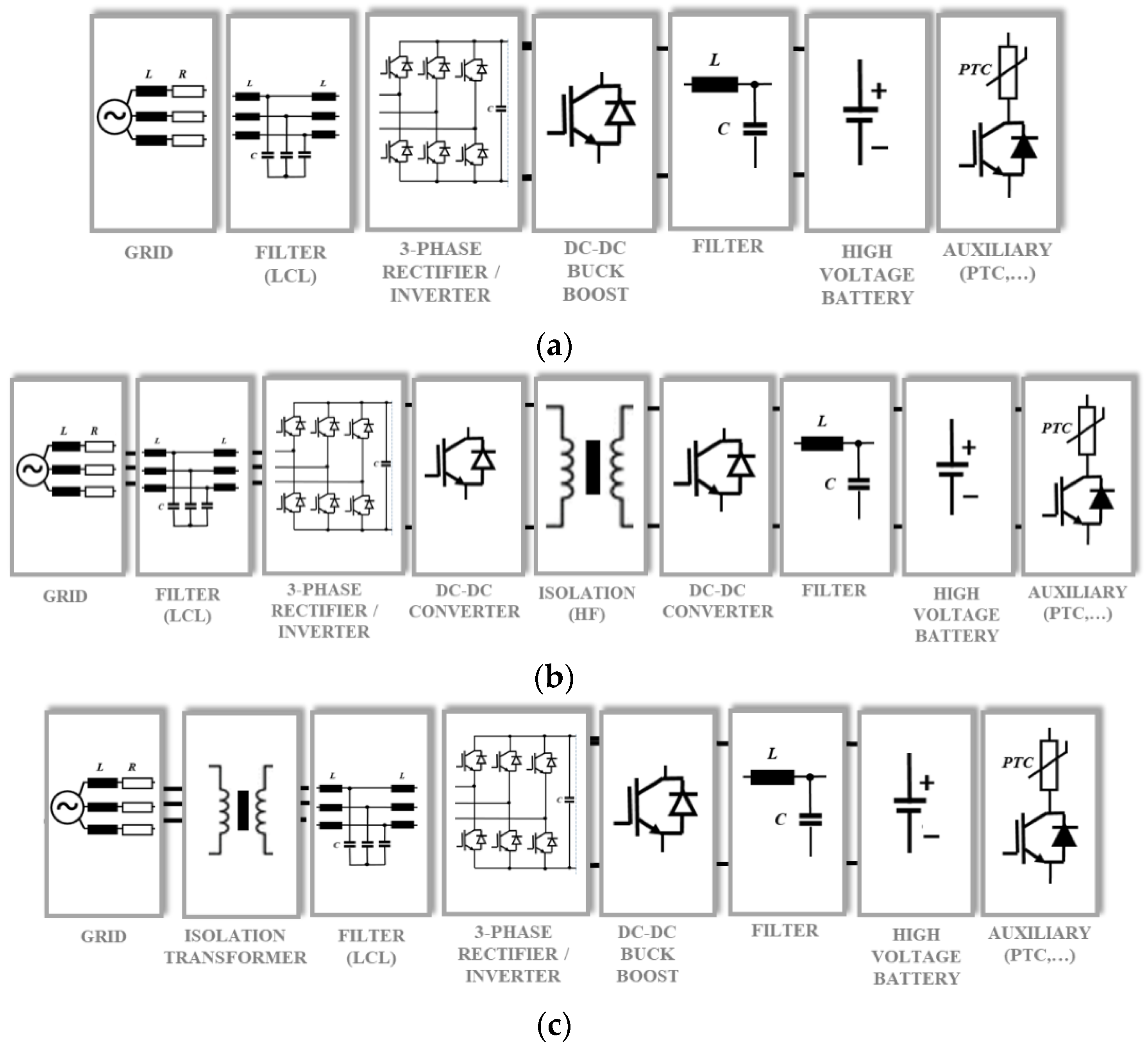
Different topologies for the realization of bi-directional charging respective bi-directional charging stations are existing. The main difference is if the DC side is isolated from the AC side respective where the isolation takes place. Depending on the topology, different measures to ensure safety on the DC side are required. Although non-isolated EVSE have an easier electronic design compared with isolated ones, the requirements in terms of safety are higher. In some cases, non-isolated bi-directional EVSE might not be compliant to national grid codes. For isolated EVSE, the isolation can either take place on the AC side via an isolation transformer or on the DC side via a high-frequency (HF) transformer. Benefit of using HF transformers are the higher efficiency and the lower weight compared with isolation on AC side using an isolation transformer.

Figure 1 shows the electronic design of a bi-directional EVSE having no-isolation between AC and DC side (a), using an isolation transformer on the AC side (b) and using a HF-transformer on the DC side (c).

The topology of the bidirectional electric vehicle charging station affects the frequency-dependent grid impedance. The individual components are explained by means of a non-isolated bi-directional EVSE.

The 3-phase AC mains represents the ohmic-inductive grid. Passive LCL filters are state-of-the art for harmonic reduction in grid-interfaced distributed power sources [7] but will impact the supraharmonic behavior and frequency-dependent grid impedance. The 3-phase rectifier/inverter circuit is connected to the mains via a LCL filter. The 3-phase PWM controlled converter maintains a constant DC link voltage and maintains reactive power control. The DC link is coupled to a buck/boost bi-directional DC-DC converter back end which finally connects to the high-voltage battery of the electric vehicle. Figure 1 shows, in addition, the connection of auxiliary HV onboard loads such as the PTC heater which can be a source of wideband supraharmonic emissions. The heater subsystem is interconnected to the HV battery through power switches [14].

2.2. Regulatory Frameworkf of Bi-Directional EVSE

From the perspective of the electrical grid, the bidirectional charging stations represent a novelty in the electrical grid. For the charging process it’s considered as a load and for discharging process it’s considered as a power generation unit. Different regulations and standards for the grid connection are applicable (Grid codes, EMC regulations). For both, EMC regulations and grid codes, the nominal power of the electrical equipment is the defining criteria regarding requirements for grid connection.

In discharge operation EVSE will be classified as “power generation unit”. In Europe the requirements for interconnection with the public grid are defined in the international and national grid codes. The Austrian market regulations for the electricity market are defined in the technical and organizational regulations (TOR). These are divided into several sections for power generation units and electrical equipment. Essentially, the requirements for discharge mode of the EVSE are described in the “TOR Erzeuger Typ A” which defines the requirements for power generation units of a nominal power up to 250 kW [16].

The bidirectional charging station under test does have a rated power for charge and discharge of 11 kW (3-phase, nominal current of 16 A) and is connected to the public grid via CEE 32 A connector. In this case, the regulation refers to the TOR D2 regulation which refers further to the IEC61000-3-2 [17] for generation units with a nominal current below 16 A [18].

In charging operation, the EVSE has to fulfill EMC standards in order to qualify for the CE mark. In Europe, the applicable standards for harmonic emissions (conducted emissions) of electrical equipment are the IEC61000-3-2 for currents below 16 A and the IEC61000-3-12 for currents between 16 A and 75 A. These standards cover emission limits up to a frequency range of 2 kHz. Above 2 kHz up to 150 kHz no emission limits exist. Consequently, the investigated charging station in both operation modes needs to fulfill the requirements of IEC61000-3-2 Class A.

2.3. Reconstructed Electrical Distribution Grid at University of Applied Sciences Technikum Wien

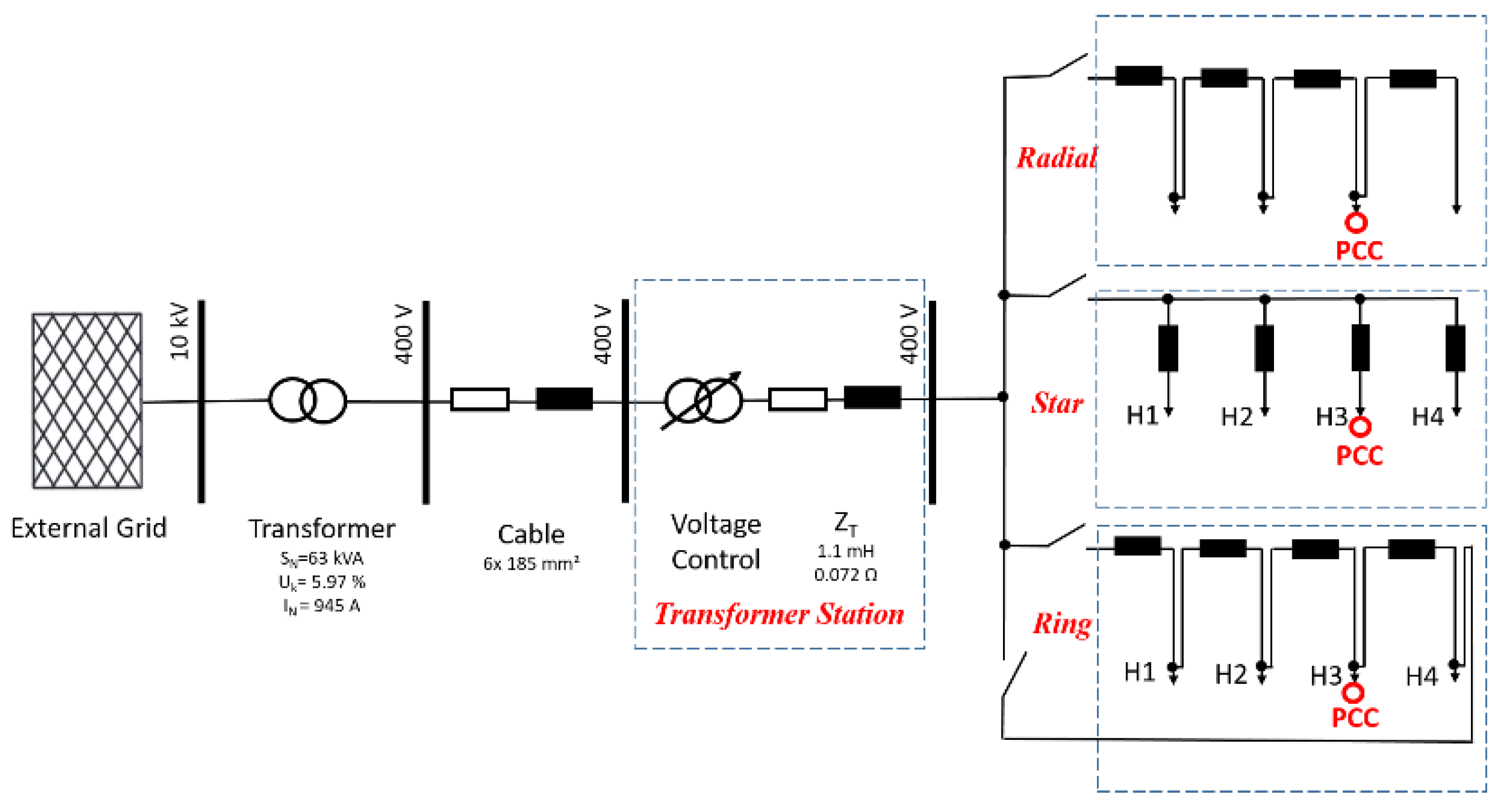
As standard laboratory, tests are executed at idealized test conditions and field tests are dependent on local conditions in this study all tests are conducted at a reconstructed electrical distribution grid. At the University of Applied Sciences Technikum Wien the first Smart Grid Lab of Austria is realized, where a typical distribution grid is recreated considering different topologies (star, radial, etc.) and grid impedances allowing operating the smart grid as rural, suburban or village grid.

The lab is connected to the public grid via a 630 kVA transformer and 6 × 185 mm² cables to ensure high short-circuit power. In the lab itself a transformer with longitudinal regulation is installed to control the line voltages independently. Furthermore, the transformer impedance of a typical transformer of the distribution grid is recreated by additional inductances and resistances. The base for choosing the typical impedances is the statistical analysis of electrical distribution grids addressed in [19]. According to [19], four different types of distribution grids are defined: urban, suburban, village and rural grid. Depending on the type, different grid topologies are used. Although for suburban grids ring connections are mainly used, village grids are often realized as star and rural grids as radial topology [19]. In the Smart grid lab, all of these topologies can be implemented (See Figure 2). Up to four feeders (houses) can be connected to the recreated transformer station whether in star, radial or bus connection. For the connection of the feeders, typical line impedances based on typical cable length and diameter used in distribution grids according to [19] are recreated using inductances and resistances. Further bypassing of inductances and resistances is possible in order to recreate low and full load behavior.

The typical distance for a suburban house connection is around 17 m, for a village grid 32 m and for a rural grid 54 m from the transformer station (Weibull distribution). The typical diameter for a house connection is 50 mm², for a suburban and for a rural house connection 16 mm² NAYY cables are used. Cables from the transformer station vary between 50 mm² and 140 mm² [19].

Finally, at each feeder Prosumer houses are connected. The equipment of the individual houses covers photovoltaic systems, battery storage systems, uni- and bidirectional electric vehicle charging stations, heat pumps and a variable load in order to simulate different load profiles. Further any other loads can be connected via CEE plugs (TV, lights, etc.). Figure 2 shows the single-line diagram of the smart grid lab.

The point of common coupling (PCC), where the bi-directional electric vehicle charging station is connected, is shown in Figure 2 for the different grid topologies. Investigations for radial-connection will represent realistic results for rural areas and for ring/star connection for a suburban/village area.

One main benefit of using the reconstructed electric distribution grid is that all components are well known. Influence of other electrical equipment and interactions are avoided when operating only one electrical equipment at a time.

2.4. Measurement Instruments

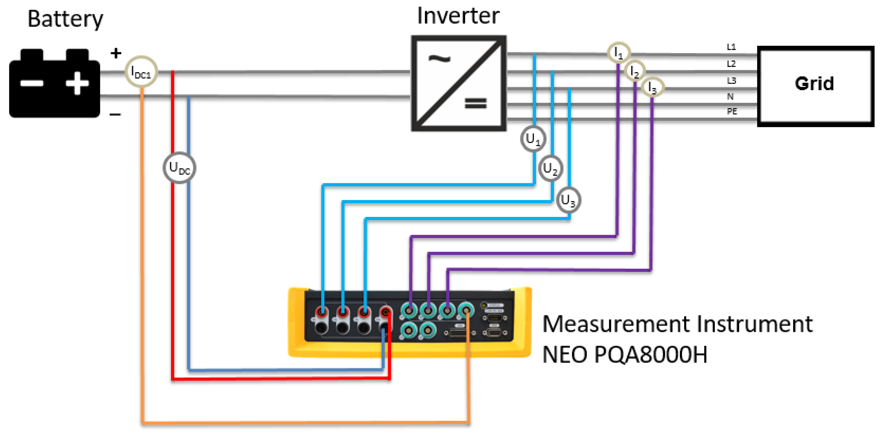
For the measurement of the supraharmonics the NEO PQA8000H Power Quality Analyser and the DS Sirius-HS for raw data recording are used. Both instruments offer a sampling rate of 1 MS/s per channel with a basic accuracy of 0.05%. For the measurement of the currents Rogowski coils are used with high-bandwidth (1 MHz) and a basic accuracy of 1% (calibrated to 0.3%). The PQA8000H is used with a 500 kHz analog filter. The DS Sirius-HS only offers a 100 kHz analog filter; therefore, no filter is selected. The measurements are repeated and recorded multiple times in order to ensure reproducible results.

For measurement of the grid impedance, the IMD 300/1 Grid impedance analyser of Spitzenberger and Spies and the RSIA Grid Impedance Analyser [20,21] are used, which are capable of measuring the high-frequency grid impedance up to 150 kHz. The principle is based on signal injection at particular harmonic orders (h) via a current source. The grid impedance of the harmonic is calculated using Ohm’s law assuming Thevenin’s equivalent of the remaining network [3]. Voltage and current of each harmonic are measured before and during signal injection and the grid impedance for the particular harmonic is calculated according to (1):

$$Z_{\mathrm{i}}=\frac{\mathsf{\Delta }{U}^h}{\mathsf{\Delta }{I}^h}$$

(1)

For the measurement of the efficiency and other power quality parameters, the NEO PQA8000H instrument is used. The harmonics are measured using the NEO PQA 8000 Power Quality Analyzer which is compliant to IEC61000-4-7 [22] and IEC61000-4-30 Ed.3 standard [23]. The measurement instrument stores gapless 10/12 period values, synchronized to the mains frequency. Figure 3 shows the measurement setup for the power quality (AC) and efficiency measurements (AC and DC).

The following table (

Table 1. Accuracy of measured parameters.

Measurement	Accuracy <100 Hz [%]	Accuracy 100 Hz–10 kHz [%]	Accuracy 10 kHz–150 kHz [%]
Voltage	0.05	0.10	0.50
Current	1.00	2.00	5.00
Power	1.00	2.00	5.03
Grid Impedance	2.00	5.00	10.00

) gives an overview about the accuracy for the individual measurement parameters.

Accuracy values for voltage and grid impedance are take from the manufacturer’s datasheet. The accuracy for the current and power measurement is calculated according to ENV13005 [24] using rectangular distribution and a weighting factor of 0.58.

2.5. Signal Processing Harmonics and Supraharmonics

2.5.1. Fourier Transform

Each signal can be presented in the time domain or in the frequency domain. The Fourier transformation is used to transform a signal form the time domain in the frequency domain and distorted signal waveforms (voltage, current) can be decomposed into several sinusoidal signals. The representation of the sinusoidal signals in the frequency domain can be shown according to (2) [25,26]:

$$f\left(t\right)=c_0+{{\displaystyle \sum }}_{k=1}^{\infty }{c}_k\times sin\times (\frac{k}{N}\times \left(2\times \pi \times f_1\right)\times t+{\phi }_k)$$

(2)

The signal is decomposed into the DC component c₀ and a number of sinusoidal signals where f₁ is the fundamental frequency, k is the order of the spectral component, N is the number of fundamental periods, c_k is the amplitude respective φ_k the angle of the spectral component.

The output of the FFT for analysis of harmonics and supraharmonics is processed differently according to IEC61000-4-7 [22] and IEC61000-4-30 Ed.3 [23] standards.

2.5.2. Total Harmonic Distortion (THD_i) and Total Demand Distortion (TDD)

For characterization of the overall harmonic distortion of a signal the THD_i and TDD calculation is used. The Total Harmonic Distortion (THD_i) references the harmonic current content of a signal (I₂…I_n) to the fundamental of the signal (I₁). In this paper the THD was calculated up to the 50th Harmonic and given by (3)

$${THD}_i=\frac{\sqrt{I_2^2{+I}_3^2{+I}_4^2{+I}_5^2+\text{…}}}{I_1}$$

(3)

The Total Demand Distortion (TDD) references the harmonic content of a current signal (I₂…I_n) to the nominal current (I_L) of the equipment. The TDD factor is defined in IEEE519 and given by (4):

$$TDD=\frac{\sqrt{I_2^2{+I}_3^2{+I}_4^2{+I}_5^2+\text{…}}}{I_L}$$

(4)

2.5.3. Supraharmonics According to IEC61000-4-7

According to IEC61000-4-7, all sampled data are split into a time-window of 200 ms (not synchronized with the grid frequency). After applying a high-pass filter to the signal, a Discrete Fourier Transformation (DFT) with rectangular time window is applied. As output of the DFT the amplitude and phase angle for each frequency component (5 Hz) are available which finally are grouped into 200 Hz bands. A detailed description is available in [22]. The standards define a range from 2 to 9 kHz for grouping the frequency components. Nevertheless, in this study, this grouping method is used up to 150 kHz and compared with the measurement method according to IEC61000-4-30 Ed.3.

2.5.4. Supraharmonics According to IEC61000-4-30 Ed.3

According to IEC61000-4-30 Ed.3, all sampled data are split into a time-window of 10-periods synchronized with the grid frequency. The recommended sampling rate is 1024 kHz. A high-pass filter (analog or digital) is applied on the signal and 512 samples are used for the FFT analysis. This results in a 0.5 ms measurement interval. The standard proposes a constant gap resulting in only 8% covered data for the supraharmonic measurement. All frequency components finally are grouped in 2 kHz bands starting at 9 kHz up to 149 kHz [23,27].

The non-gapless data processing represents a main disadvantage of this method. In [27] a minimal measurement interval of one-cycle for the measurement method according to IEC 61000-4-30 is recommended to increase the accuracy of this method.

In this study the measurement procedure of IEC61000-4-30 Ed.3 is adapted to a non-gapless method maintaining grouping into 2 kHz bands.

2.5.5. Demonstration of Higher Frequency Measurement Data above 9 kHz

For lower frequency harmonic emissions, the harmonic contents are typically shown as RMS values for current/voltage or as percentage of the fundamental.

Although for conducted emissions, voltage and current are typically shows as percentage of the fundamental or as RMS values, for higher frequency data, the units dB_µA respective dBµV are used. This data representation is used by different standards such as the IEC61000-2-2:2020 [28]. The equation is shown in (5), according to [3].

$${\frac{{\mathrm{I}}^{\prime }}{{\mathrm{dB}}_{\mu \mathrm{A}}}}_{}=20\times {\log }_{10}\frac{\mathrm{I}}{1 \text{µ}\mathrm{A}}$$

(5)

A value of 1 A will correspond to a value of 120 dB_µA and 1 μA will correspond to 0 dB_µA.

2.6. Efficiency

The efficiency of the V2G charger is measured with a high-precision power analyser (NEO PQA8000H). The active power is directly calculated by the instrument and the integration interval for energy calculation can be defined by the instrument. In this study the active power is calculated based on 200 ms values and the integration time was defined with 2 s. The measurement instrument considers the full harmonic and supraharmonic spectra for active power calculation with a bandwith of 500 kHz. The energy is calculated out of the 200 ms power values (integration). To determine the efficiency of the V2G charging station three different efficiency values are caclulated. To measure the AC power all three phase voltages and currents are measured at the connection point of the V2G charger (CEE socket). For the DC power the DC voltage and current at the output of the V2G charger (cable with Chademo connector) are measured. The voltages are measured directly (0.05% accuracy), whereas the currents are measured using AC/DC clamps (0.3% accuracy).

The AC to DC efficiency (charging the vehicle from the grid) is calculated according to (6) where P_DC represents the active power and E_DC the energy from the vehicle battery. P_AC represents the active power and E_AC the energy of the electrical grid.

$$ɳ=\frac{P_{DC}\left(t\right)}{P_{AC}\left(t\right)}\times 100=\frac{E_{DC}}{E_{AC}}\times 100$$

(6)

The DC to AC efficiency (discharging the vehicle) is calculated according to:

$$ɳ=\frac{P_{AC}\left(t\right)}{P_{DC}\left(t\right)}\times 100=\frac{E_{AC}}{E_{DC}}\times 100$$

(7)

In order to determine the Roundtrip efficiency also the charging-discharging losses inside the battery need to be considered. The round-trip efficiency considering all losses (AC to DC, charge–discharge, DC-AC) is calculated out of the ratio between the energy from the grid to the vehicle battery (E_charge) and the energy from the vehicle battery to the grid (E_discharge). The charging and discharging losses can be calculate according to (8). The charging process has to start at the same SoC value as the discharging process stops.

$$ɳ=\frac{E_{charge} }{E_{discharge}}\times 100=\frac{E_{AC}}{E_{DC}}\times 100$$

(8)

To ensure that the SoC at beginning of the charging process is the same as at the end of the discharge process, the V2G charger was controlled by the Open Charge Point Protocol (OCPP) communication. Figure 3 shows the measurement setup for the power quality measurements and efficiency measurements.

2.7. Control of the Charging Station

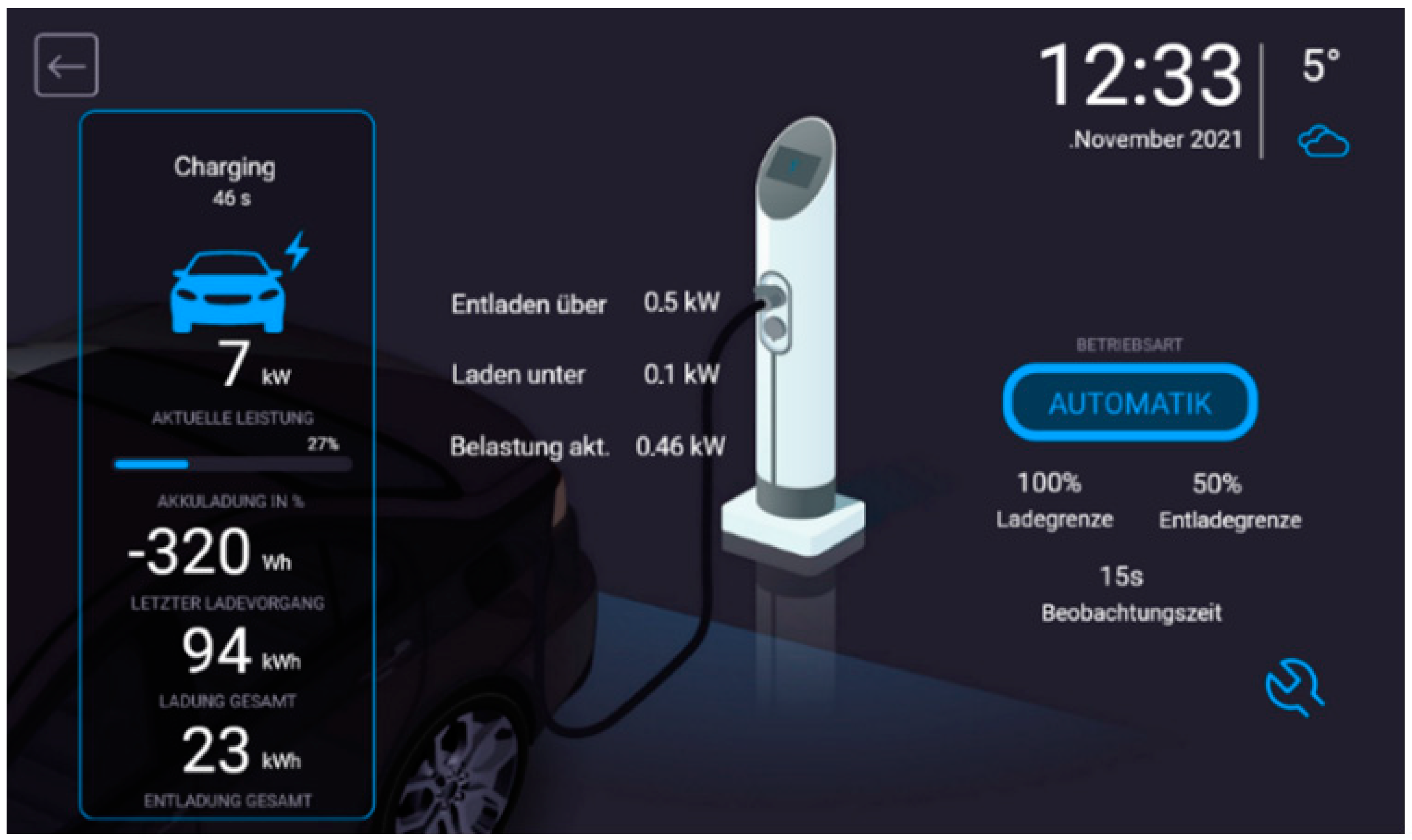
In order to operate the EVSE at different power levels, the charging station was controlled via the OCPP version 1.6, which allows static and dynamic control of the EVSE. The OCPP is a communication protocol between a charging station and a central system. The standard ensures interoperability of systems of different manufacturers and avoids proprietary, manufacturer-specific protocols [29].

In this study, a special OCPP server was programmed to operate the EVSE remotely by manual set point definition. Figure 4 shows the user interface of the OCPP communication.

3. Power Electronics and Supraharmonic Emissions

Harmonic disturbances (voltage and current) in a frequency range above 2 kHz up to 500 kHz are called higher frequency (HF) or supraharmonic Emissions [5]. Although origin, propagation and mitigation of low-frequency emissions (up to 2 kHz) are well researched, for supraharmonic emissions further research is required and recommended by multiple studies [3,7,10,12].

3.1. Sources of Supraharmonic Emissions

In the past, mostly passive power electronic converters are used such as diode or thyristor converters which mainly cause low-frequency emissions (typically up to 2 kHz).

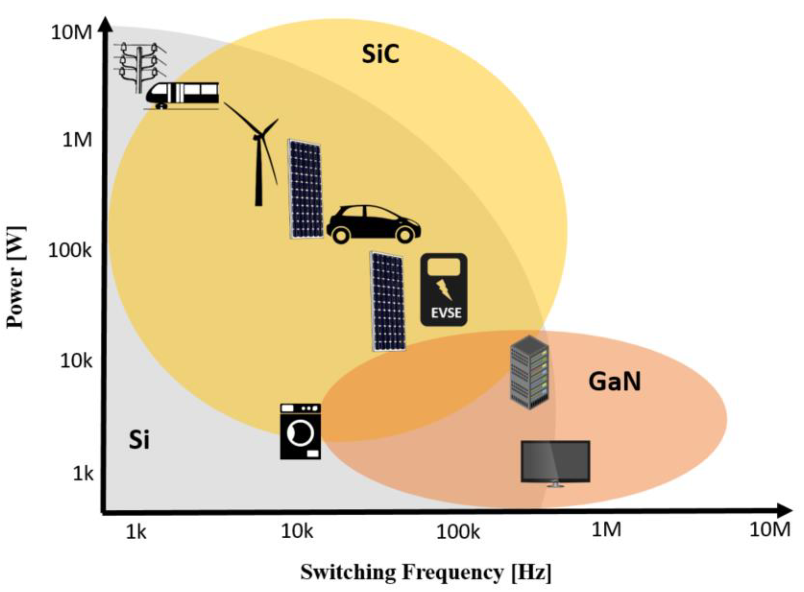
The use of active power electronics for AC-DC conversion with high switching frequencies (such as MOSFET, IGBT, etc.) improves power efficiency [30]. Nevertheless, these technologies reduce lower harmonic distortion but increase higher frequency emissions, above 2 kHz. For conductive power transfer, switching frequencies up to 40 kHz are used, whereas for inductive power transfer (wireless charging stations) switching frequencies up to 300 kHz are used [3]. As emission limits above 150 kHz are stricter than at low frequencies, the switching frequencies are often chosen in order to keep harmonics of it below 150 kHz [5]. Figure 5 shows typical switching frequencies (x-axis) of silicon (Si), silicon-carbid (SiC) and gallium-nitride (GaN) technology, depending on their power level (y-axis) [31].

3.2. Effects of Supraharmonics

Possible effects of supraharmonic Emissions are quite diverse. Already, small voltages in the higher frequency range cause significant thermal stress to electronic equipment and consequently increase losses (due to the skin effect) and reduce lifetime. Malfunction of electronic devices are reported as well as acoustic noise emission and Flicker. This effects already take place at very small supraharmonic voltage levels of about 1% of the fundamental voltage [30]. In [5], it is shown that a large supraharmonic current flow of a high-power electronic device (e.g., EV charger) to a low-power electronic devices (e.g., TV, notebook or LED) cause malfunction or damage to the low-power device as the supraharmonic current is relatively high compared with its nominal power [12].

The supraharmonic distortion directly influences the power and energy losses in the electrical equipment. In [32] it is shown that the power losses can reach several percent of the power at fundamental frequency. Tests in [33] show that LED streetlamps increase or decrease illuminance at the presence of supraharmonic voltages.

Overloading of distribution transformers [12], capacitor bank overload, EMC filter overload [33], failure in cable terminations due to resonances [34], resonances at voltage source converters (VSC) with 500 m cable [35] and increased heat in series elements are further reported effects.

3.3. Missing Regulations

At above 2 kHz up to 150 kHz, no standards defining emission limits currently exist. Currently only emission limits in this frequency range are existing for some devices such as for lighting [27]. In [3,12,36] the missing limitations for higher frequency current emissions are emphasized. Above 150 kHz EMC standards such as EN55011 [37] are applicable for symmetric disturbances. Asymmetric disturbances such as those described in IEC61000-4-16 [38] are not considered in this study.

Both the measurement procedure as well as emission limits are subject of discussions in standardization committees.

The measurement procedure for high-frequency EMC tests is different to low-frequency emissions. Low-frequency emissions are based on fast Fourier transform (FFT) of the digitized sampled values of voltage and current. This is the base for calculations in standards such as the IEC61000-4-7 [22] or IEC61000-4-30 Ed.3 [23]. The measurement in the frequency range between 2 kHz to 2 MHz is based on quasi-peak detectors. Quasi-Peak detectors emulate human hearing, and the design is focused on analog radio communication [12]. Seeing as nowadays, digital communication such as the Power Line Communication (PLC) is taking over substantial importance in the electrical grid, the measurement procedure based on quasi-peak detectors is not sufficient anymore.

EMC tests based on quasi-peak detection are executed at an artificial line impedance stabilization network (LISN) with an impedance of 50 Ω. This high value and the idealized high-frequency grid impedance does not represent realistic grid conditions. Furthermore, all tests are executed one-by-one and possible equipment interaction between devices is not considered at all [12].

3.4. Propagation of Supraharmonics and Primary vs. Secondary Emissions

To characterize supraharmonic emissions, it is important to distinguish between primary and secondary emissions. Primary emissions are emissions generated from the device depending on its output impedance. This impedance includes grid impedance, filter of the device and impedance of other connected devices (EMI filter). Secondary emissions are generated elsewhere and propagate due to the low impedance path to the terminal of the device [10]. Secondary emissions grow by number of devices connected close-by [7]. The emissions of a device at a particular frequency are the sum of the primary and secondary emissions, which complicates the separation of them using data of field tests.

The measured supraharmonics in [33] of an LED streetlamp connected at the field and at a lab shows a completely different waveform and spectra for the current. In [39], it is shown that a high voltage at supraharmonic frequency is present at an electric vehicle charging station even if no EV is connected for charging. In [3,27], the propagation of supraharmonics is explored mainly as a local phenomenon where supraharmonic emissions will affect equipment connected close to the source (low-impedance path). In [40], interactions between two electrical devices are described, where oscillations due to parallel connected EMC filters occur. In [10], it is shown that supraharmonic emissions of multiple EV chargers are staying inside an installation and no supraharmonic power flow back to the transformer station could be detected. Nevertheless, in [41], supraharmonic emission of components were shown to propagate over distances of 16 km in the medium voltage grid.

In all cases, the frequency-dependent grid impedance plays an essential role for propagation of supraharmonic emissions. Therefore, all investigations in this study cover both, supraharmonic emissions and high-frequency grid impedance measurements.

3.5. High Frequency Grid Impedance

The frequency-dependent grid impedance determines the power flow of supraharmonic emissions whether they flow back to the transformer station or stay within an installation.

Simulations of the frequency-dependent grid impedances differ strongly from real values. Although the low-frequency grid impedance mainly depends on components of the electrical grid such as transformers, line impedance, reactive power compensation units, etc., the high frequency grid impedance is strongly affected by electronic loads and power sources connected, and varies by time [30].

In [42], it is shown that the grid impedance in the harmonic frequency range (<2 kHz) mainly depends on the components of the electrical grid. The grid impedance in the frequency range from 10 to 150 kHz is mainly affected by high-power electronic equipment (motors with VFD, PV systems, EVSE) and the grid impedance in frequency range above 500 kHz is affected by low-power power electronic equipment (power supplies, lighting, etc.). Only results out of a few field tests exist which might be related to the lack of suitable measurement equipment [10] and the need of further research is outlined in [3,5,10,30].

3.6. Wideband and Narrowband Emissions

Supraharmonic emissions are separated between narrow-band and wide-band emissions. Narrow-band emissions are emissions with a small bandwidth of a few spectral lines (<1 kHz) and a high amplitude, whereas wide-band emissions spread over multiple spectral lines with lower amplitude. Source of narrow-band emissions are PWM-modulated devices [3]. Wide-band emissions are often caused by PWM-controlled devices using active power factor correction [3]. Wide-band emissions especially affects digital communication. The emissions at multiple frequencies results in a high noise floor [12]. Furthermore, the probability of generating secondary emissions at equipment connected close by is increased due to the wide-band emissions.

3.7. Modelling of Supraharmonics

Existing grid modelling software solutions often do not consider the consumer side and their electronic equipment. Only elements of the electrical grid such as transformers, cables, power lines are considered for power quality simulations. Assessments for connection of new electrical equipment to the electrical grid (grid codes) are based on calculations out of the fundamental grid impedance only [16] and the frequency-dependent grid impedance is not considered.

The typical approach of modelling a network is by using the Thévenin equivalent considering a voltage source and a RL impedance series. Usually, these parameters are calculated out of the voltage level and the short circuit power at the PCC. For low-frequency simulation capacitors are often neglected [43].

Nevertheless, for high-frequency (HF) models, the capacitors need to be considered. In [43], different methodologies are analyzed to characterize the electrical grid using a set of RLC branches. Although this approach gives a realistic model of the frequency-dependent grid impedance for the electrical grid and its components, for investigations of emissions (primary, secondary) the connected equipment at the PCC needs to be considered as well. Furthermore, modelling of narrow-band and wide-band emissions might be considered separately.

In [7] the high-frequency grid impedance is modelled using following simplifications: (1) Using Current source for DC/DC converters, (2) Replacing the inverter with three voltage sources generating the same harmonics, (3) considering the LCL filter at grid side [7]. This approach requires detailed information about the circuit of the EVSE. Further the model of the grid at the PCC and of the connected equipment needs to be known.

In [3] a simplified model using the Thévenin equivalent via a source and sink model is considered. This approach allows modelling the EVSE as a black box without knowledge of internal electronics and circuits, as input parameters for the models’ measurement data of a particular EVSE respective data of measurement campaigns are used. This approach is used for modelling of narrow-band emissions.

In [10], a simplified model is used, where each particular harmonic is represented as a current source considering the internal impedance of the emitting device itself, the internal impedance of other connected equipment and the grid impedance. Background emissions from the grid are modelled as the voltage source.

4. Results out of the Tests at the Reconstructed Distribution Grid

For all tests executed, only the V2G charging station is connected to the electrical distribution grid at the same time to avoid influence and interaction with other electrical equipment. All measurements are repeated multiple times to ensure reliable and reproduceable results.

4.1. Charging and Discharging Profile

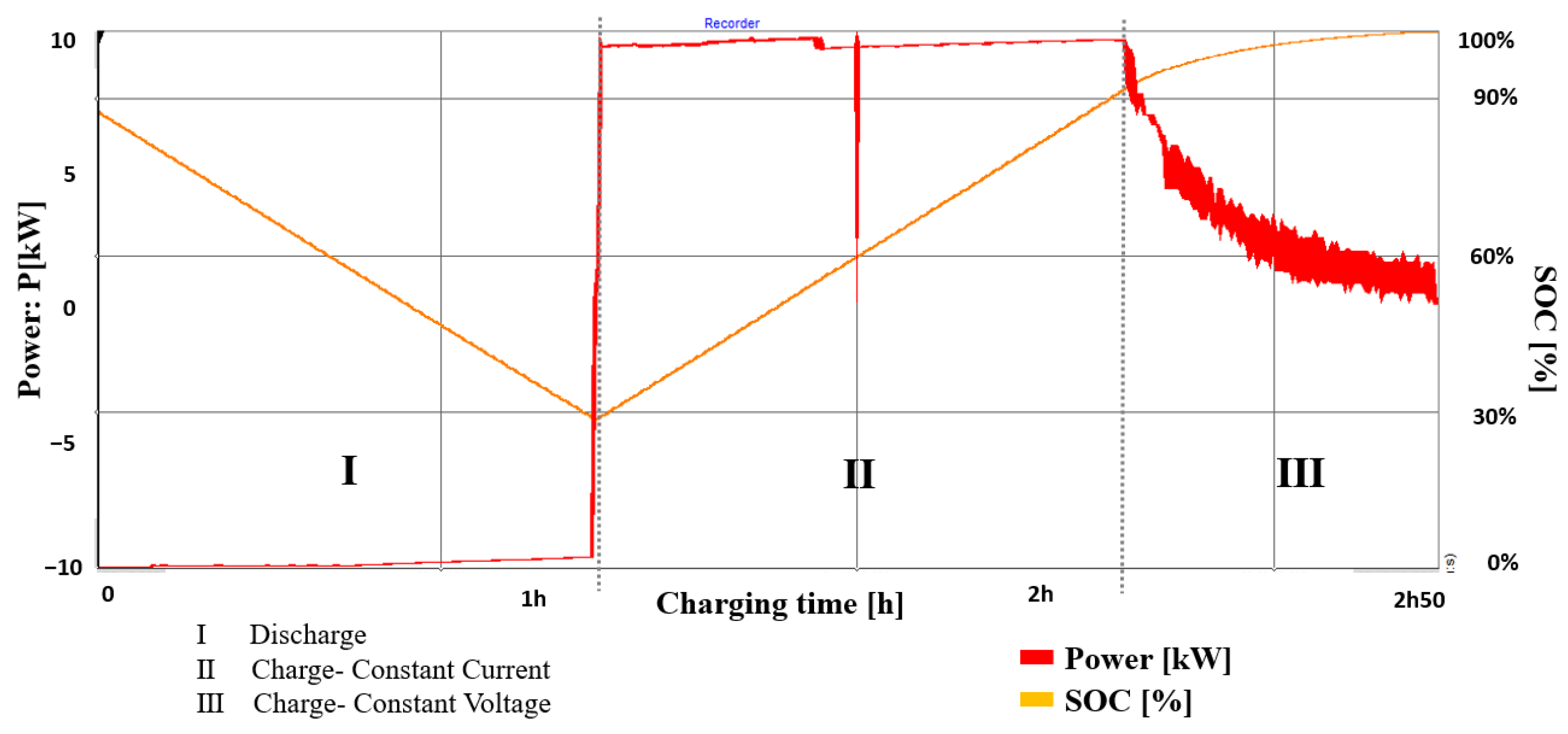
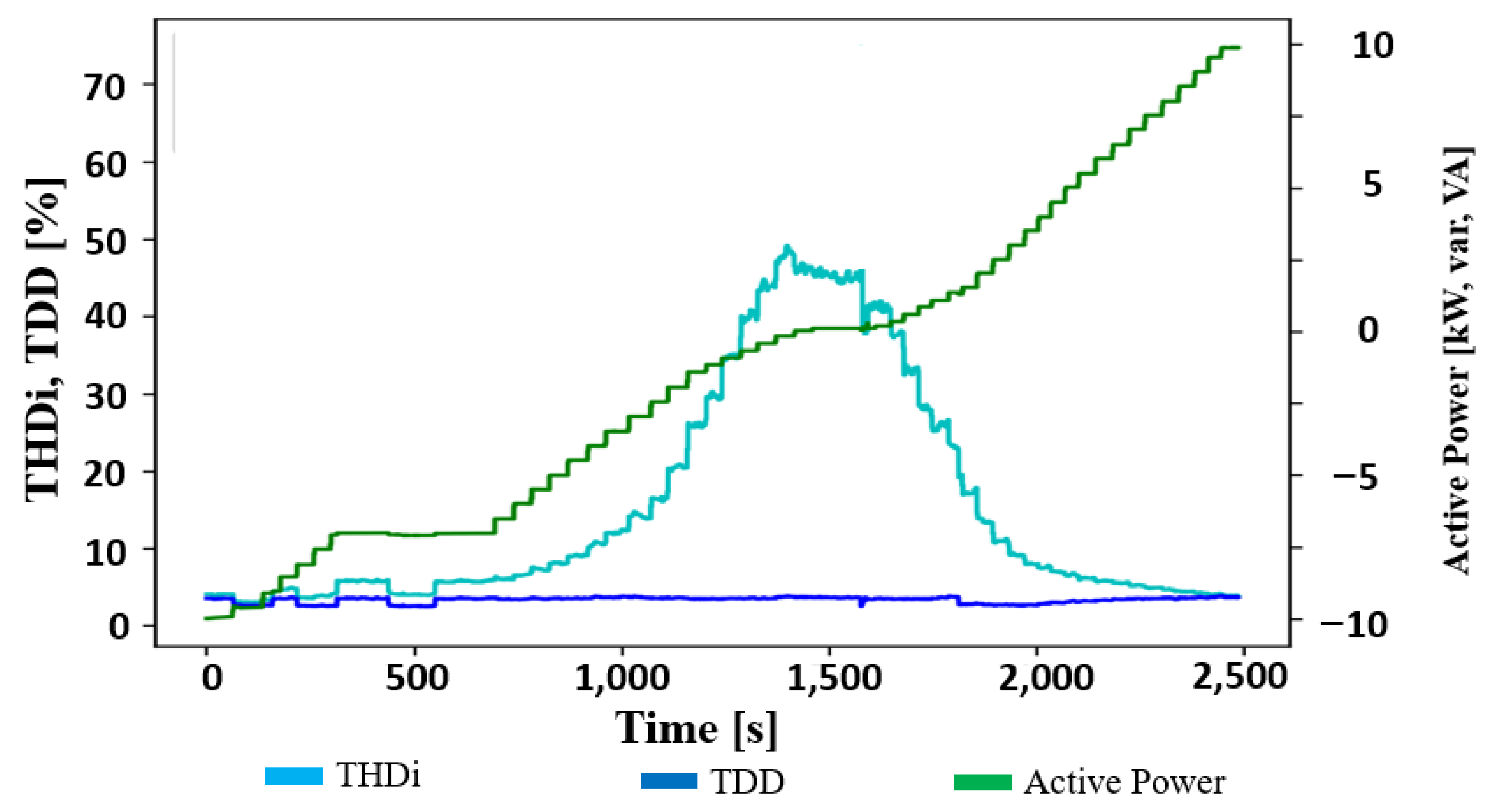
For the tests, a Nissan Leaf with a battery capacity of 30 kWh is connected to the bidirectional EVSE. The maximal charging and discharging power are rated at 10 kW. Figure 6 presents the discharging and charging profiles of the bidirectional charging station. The measurements are executed for whole charge–discharge cycles and repeated. Discharge is possible only to 30% SoC of the battery. Section I shows the constant discharging of the vehicle until 30% SoC. In Section II, the constant current phase (CC) of the charging station is illustrated. Section III shows the constant voltage phase (CV) from 93% to 100% state of charge. Particularly noticeable in the constant voltage phase is the power control of the charging station, which fluctuates by up to 20% (2 kW) within seconds. The measurement displays that the vehicle needs 38 min from 93% to 100% state of charge (2 kWh), whereas it only takes 63 min from 59% to 93% SoC (10.3 kWh) in the constant current phase at 10 kW charging power [15].

4.2. Harmonics, THD and TDD

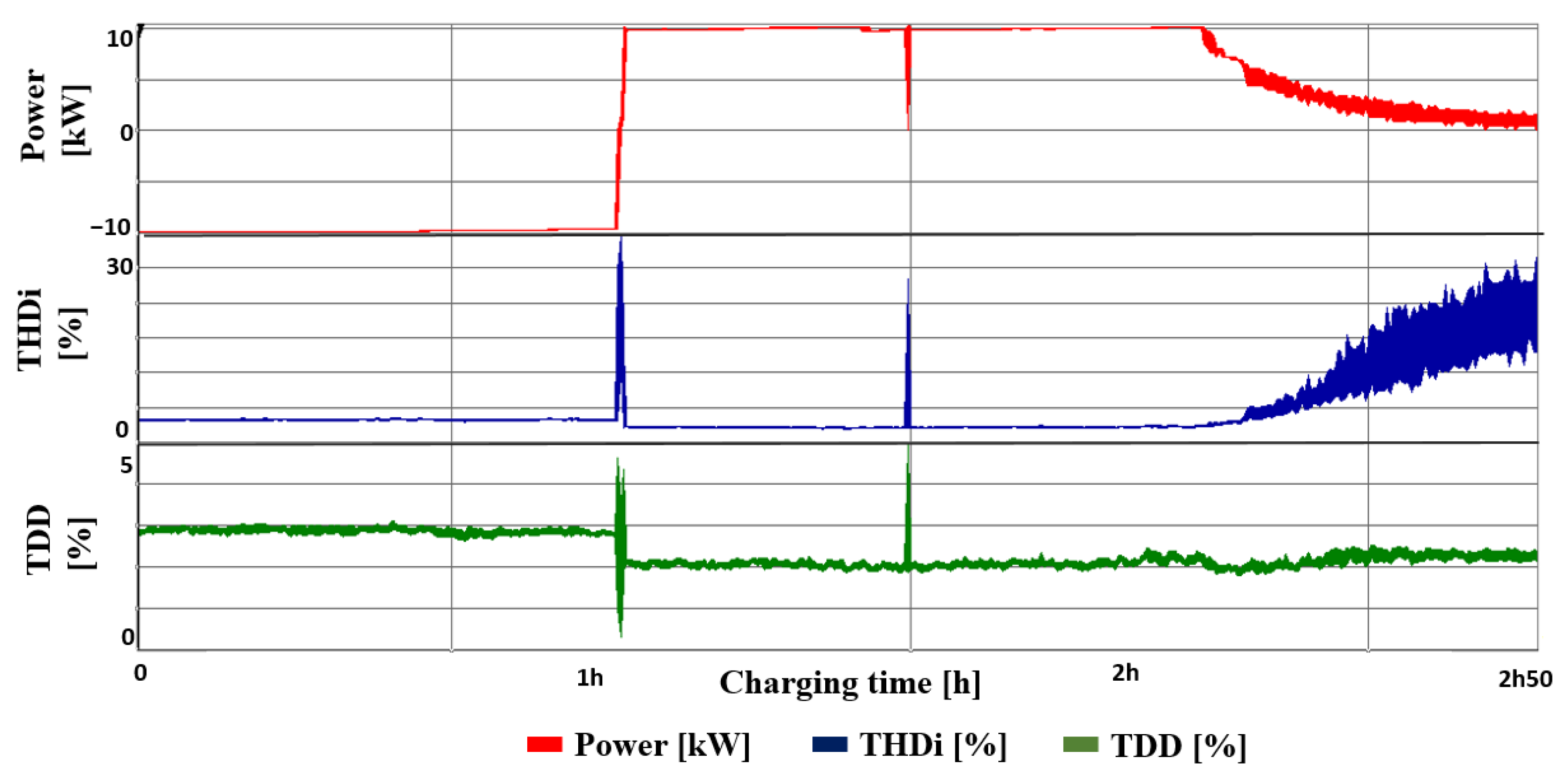
The Harmonics, THD and TDD are measured in two different operating modes-during standard charging and at individual power set point operation. Figure 7 shows the total active power for the standard discharge and charging process, the THD_i and the TDD.

The values are analyzed for the three different charging/discharging profiles. During discharging the THD_i and TDD remains stable at around 3%. In the CC phase both values are constant around 2.2%. In the CV phase, the TDD remains constant at 2.4%, whereas the THD_i rises up to 28%. The heavy variations at the THD_i which can be seen at the end of the chart are explained by the strong power variations in CV phase of charging process. 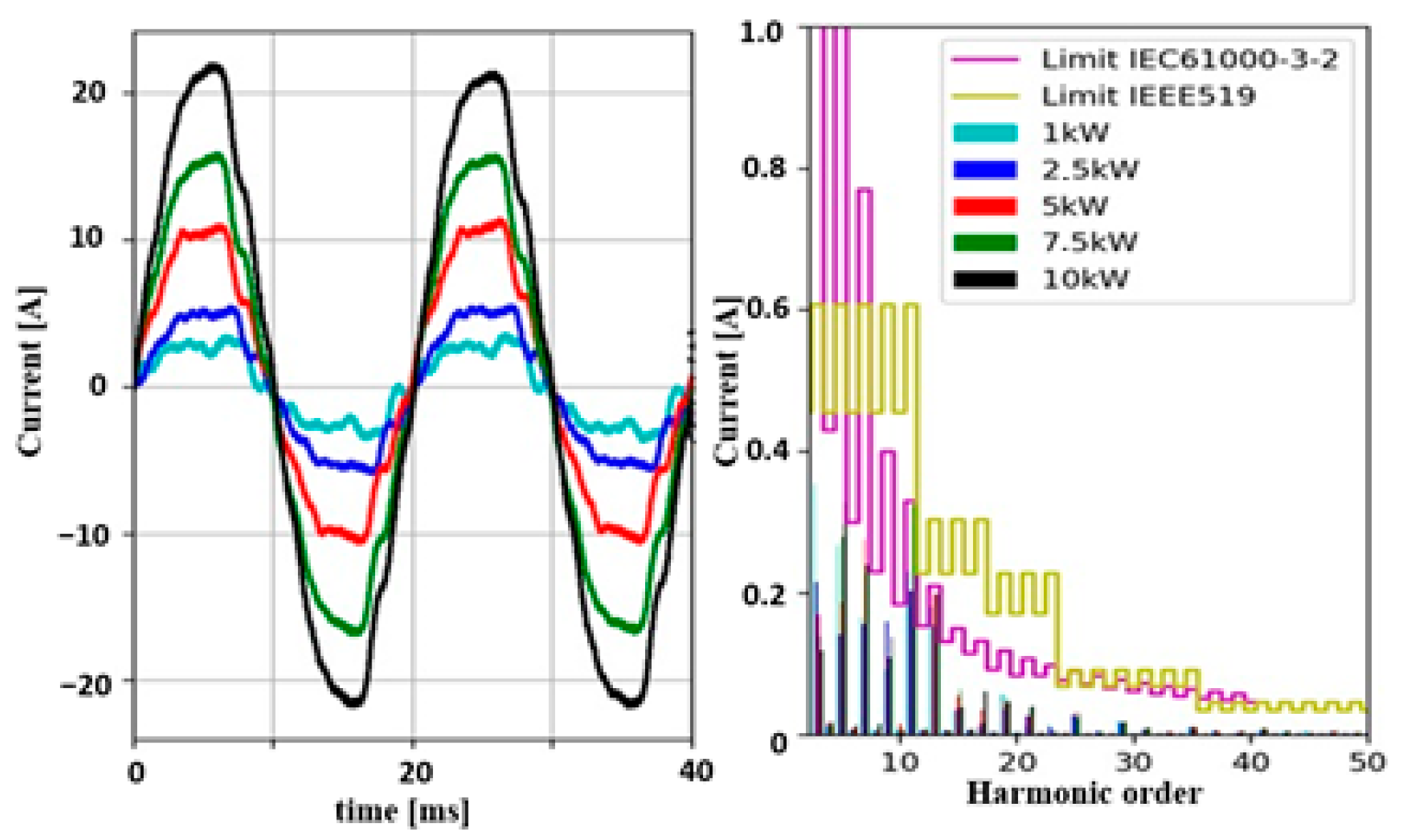Figure 8 shows the current waveform and harmonic spectrum analysis, operating the EV charging station at power set-points controlling it by OCPP communication. The results are similar for charging (constant current) and discharging, therefore only the results for charging are displayed.

As shown in Figure 8, reducing the power set point increases the relative emissions of harmonic currents and the THD_i. The distortion is significantly notable in the waveform chart (left). The harmonic emissions are constant (right) at the different power set-points.

Essentially, for all power set points the limits out of the IEC61000-3-2 and IEEE519 standards are met (95% quantile), but the THD_i can reach values up to 50% at very low power levels (<1 kW). Furthermore, considering low charging power charging instead of nominal charging (10 kW) the IEEE519 limits are violated at all power levels < 5 kW. The following table (

Table 2. THD_i vs. active power [15].

Active Power [kW]	THDi [%]	TDD [%]
10	3.8	2.9
7.5	5.4	2.9
5	8.5	2.8
2.5	17.1	2.8
1	34.7	2.8
0.5	48.4	2.7

) shows the THD_i at different power set-points.

Figure 9 shows the THD_i and TDD at different power set-points. The TDD remains almost constant above all power set-points.

Interpretation and Discussion

Although the bi-directional EVSE causes minor harmonic emissions during standard charging process, in V2G operation it can cause major harmonic emissions at low power levels referring the emissions to the actual charging power. Analyzing power quality phenomena at different power set points is especially important considering typical future V2G/G2V applications. A typical size of a PV system for a one-family household in Austria is around 5 kWp [44]. To charge the EV with excess energy of the PV system will require the EVSE to operate at partial load.

The advantage of using THD_i is that it gives an indication of the harmonic distortion at each phase of the charging process, whereas the TDD gives a better indication of the absolut emissions into the electrical grid. The TDD references the harmonic distortion in the constant voltage profile still to the nominal current and therefore shows lower values for the harmonic distortion. The relatively high emissions of the 11th and 13th harmonic is explained by the topology of the EVSE and the grid impedance at these frequencies (see Section 4.4).

4.3. Supraharmonic Emissions

4.3.1. Supraharmonics during Standard Charging and Discharging Operation

The supraharmonics are measured at all power levels from −10 kW to +10 kW with steps of 0.3 kW. Different to the low-frequency emissions (up to 2 kHz) the measurements show that the supraharmonic emissions remain constant when changing the charging/discharging power. As the emissions are identical for all three phases, the results are only displayed for Phase A.

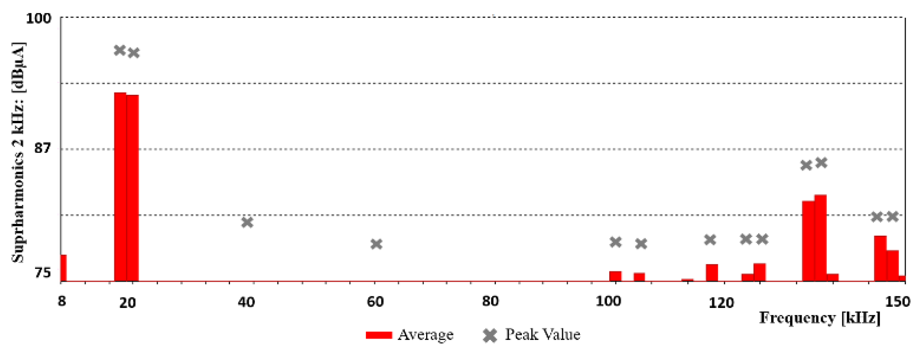
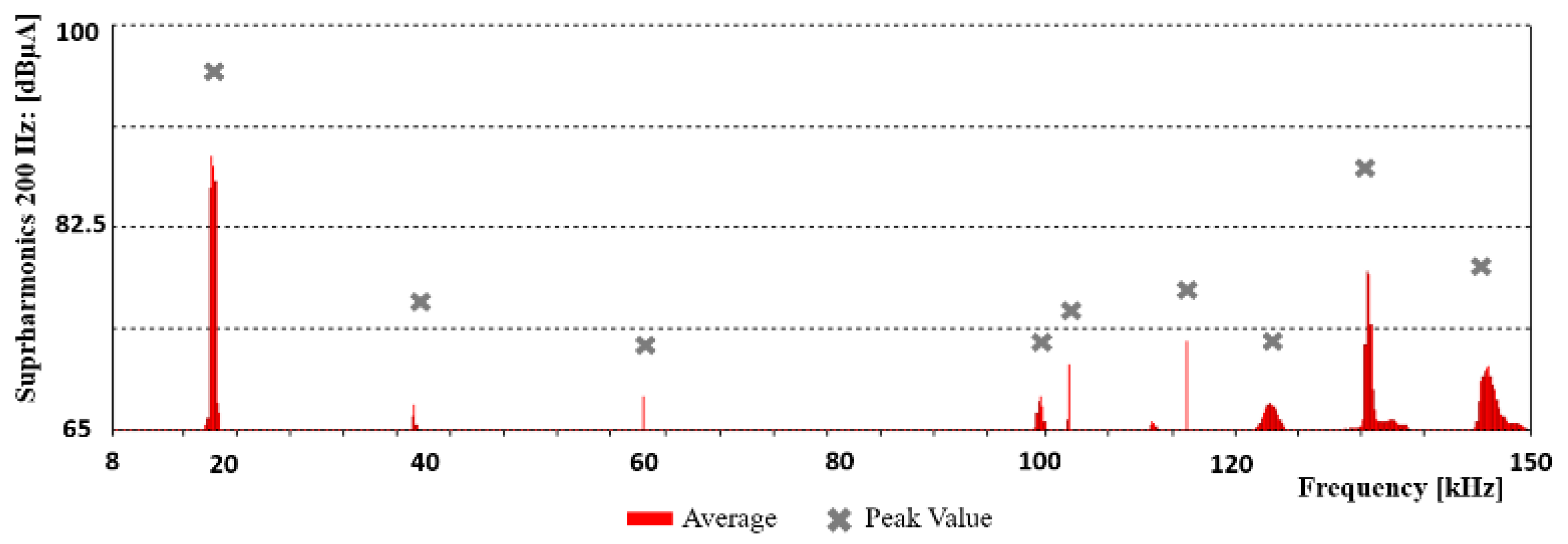
Figure 10 shows the results grouped in 2 kHz bands (IEC61000-4-30 Ed.3 modified to the gapless method) and Figure 11 grouped in 2 kHz (according to IEC61000-4-7). The red bar shows the 95% quantile, and the grey marker represents the peak value.

The switching frequency of the charging station of 20 kHz represents the highest peak with a value of 98 dB_µA at 200 Hz band grouping respective 95 dB_µA for the 2 kHz band grouping method [14]. Further peaks are notable the multiple of the switching frequencies and in the higher frequency range. The peaks in the higher frequency range are due to the DC-DC converters and auxiliary devices of the EV.

In

Table 3. Comparison of supraharmonic measurement methods by Peak value [14].

Frequency [Hz]	DFT Output 5 Hz [mA]	IEC61000-4-7 200 Hz [mA]	IEC61000-4-30 Ed.3 2 kHz (Gapless) [mA]
20	50	68	75
40	5	5	10
60	4	4	7
104	3.5	5	10
145	2	8	11

the peak values of selected supraharmonic current emissions using different grouping methods are compared.

Comparing the peak values of the different grouping methods and the output of the DFT shows that the values are heavily depending on the emission type. At narrow-band emissions, the peak values are close to each other and differ up to 15%. Wide-band emission peak values of the 2 kHz grouping method can have 2 times the value of the 200 Hz grouping method and 5 times the value of the DFT output of 5 Hz.

4.3.2. Interpretation and Discussion

Both measurement methods used are currently discussed by international standardization committees. Very likely, only one method will be used in future. The advantages and disadvantages of the different methods are shown at the application of the V2G charger.

This study shows, that even if a fixed switching frequency is used at this V2G charger both wide-band and narrow-band emissions are existing in the supraharmonic range. Although the switching frequency and its multiples generate narrow-band emissions (PWM modulation), the DC-DC converters and auxiliary loads are source of wide-band emissions. Consequently, future simulation models and synthetic signals need to consider both type of emissions.

Although the 200 Hz band evaluation method has benefits for analyzing narrow-band emission, the evaluation of wide-band emissions is challenging, as emissions are split into multiple bands. In Figure 10, this behavior is particularly notable at the wide-band emissions from 140 kHz to 144 kHz.

Furthermore, narrow-band emissions with a very small frequency band and low amplitude, can become lost in the 2 kHz grouping method. This can be seen in Figure 9 and Figure 10 when comparing the supraharmonic current emissions at 40 kHz (first multiple of switching frequency). This behavior is explained in the fact, that measurement instruments will also include the noise of the signal in the frequency band grouping.

Even if peak values of narrow-band emissions at the 2 kHz grouping method will exceed emission peaks of wide-band emissions, the averaged value of this emission can be multiple times lower or even become lost in the noise of the signal. Finally, the 200 Hz grouping method generates big amounts of data whereas a lot of data might be irrelevant if there are no emissions in that frequency range. The benefit of the 200 Hz grouping method is clearly the evaluation of narrow-band emissions as it gives information about type of emission [14,27].

4.3.3. Emissions from Auxiliary Devices Connected to the Vehicles High-Voltage System

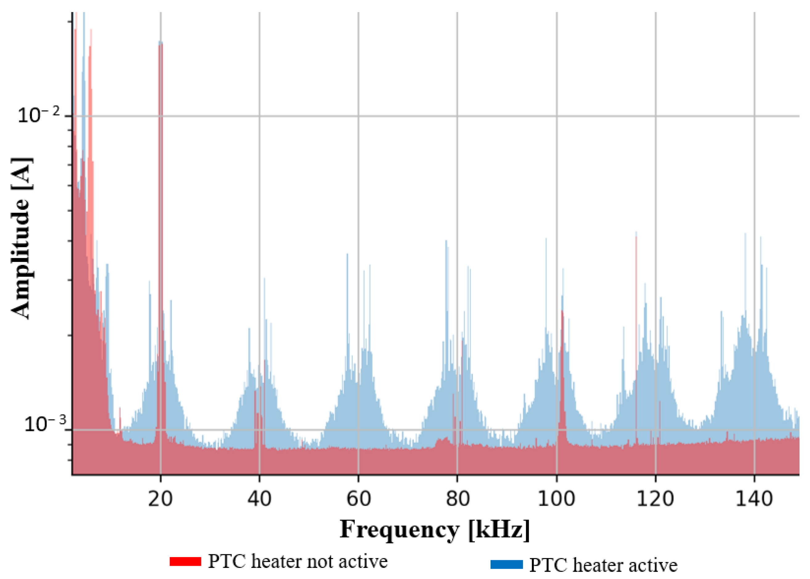
In this section, the possible influence of auxiliary loads connected to the high voltage (HV) system of the vehicle is analyzed. During the tests, the PTC heater figured out to be an additional source of emissions. In this case, the vehicle is charged (or discharged) and the PTC heater is activated at the same time, wide-band emissions are added to the frequency spectra.

In Figure 12, the supraharmonic emissions of the EVSE while charging with and without activated heater are shown.

Figure 12 shows that during the standard charging procedure, mainly narrow-band emissions are existing at the switching frequency of the EVSE and multiples of it. As soon as the heater (PTC) is activated wideband emissions appear at each multiple of the switching frequency of the heater (20 kHz) which is in the range of to the switching frequency of the EVSE. The amplitude of the emissions ranges from 1 to 4 mA. All other auxiliary loads connected to the vehicles high-voltage system do not generate additional supraharmonic emissions.

4.3.4. Interpretation and Discussion

Especially in winter times, it is very likely that electric vehicles are charged with activated heater when people are waiting inside the car for the duration of charging. This combination will cause narrow- and wide-band emissions and needs to be considered in future EMC designs and standardization. Even if the amplitude of the wideband supraharmonic emissions is very low, digital communication might be affected [12,14].

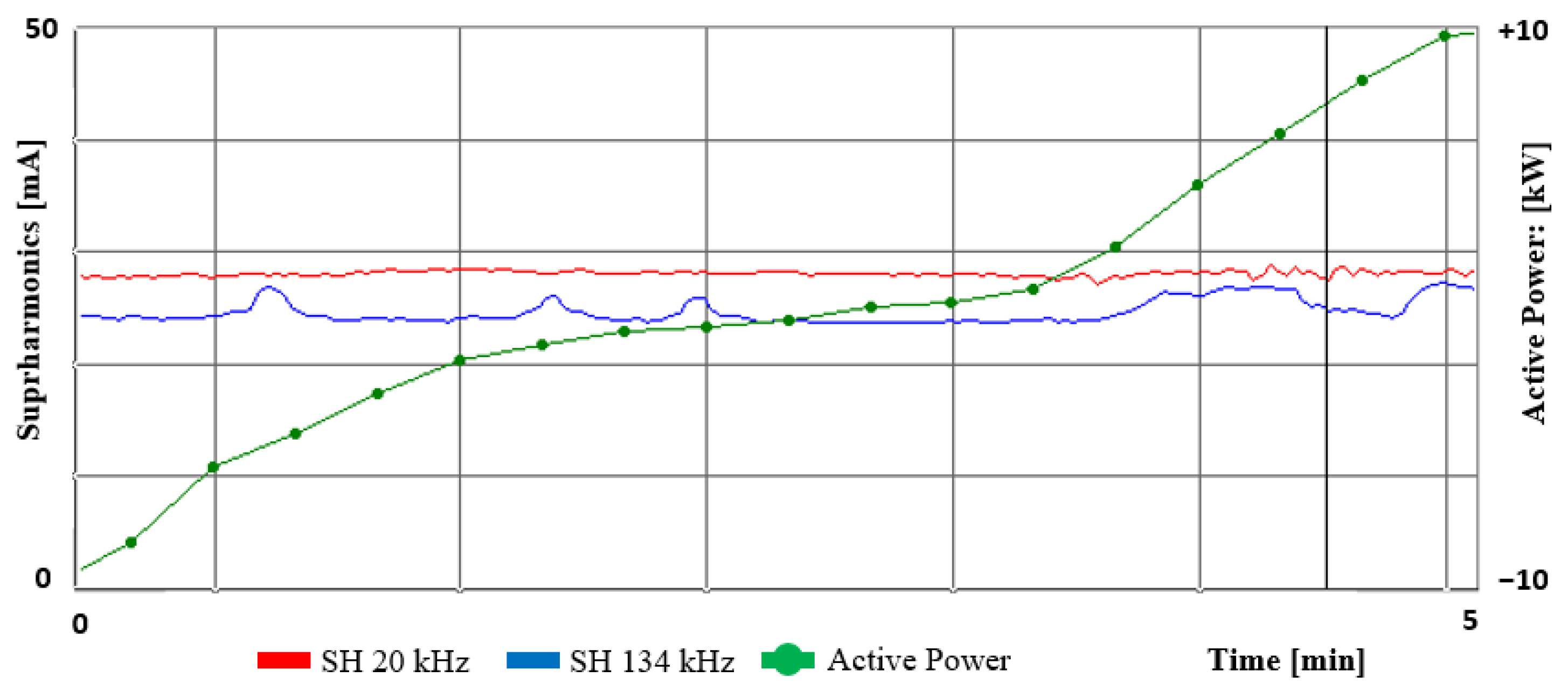
4.3.5. Influence of Charging Power

Measurements showed that low order harmonic emissions of the EVSE (up to 50th Harmonic) are strongly depending on the charging power and the grid impedance. To determine the influence of the charging power on supraharmonic current emissions the EVSE is operated at multiple power levels (controlled by OCPP communication). Figure 13 shows the power of the EVSE from −10 kW to +10 kW, the supraharmonic current emission at 20 kHz (switching frequency) and supraharmonic current at 134 kHz.

The charging power has no influence on the supraharmonic emissions. All supraharmonic emissions (20 kHz and multiples) remain stable when varying the power in charging and discharging mode.

4.3.6. Interpretation and Discussion

In contrast to low-frequency emissions in the harmonic range of up to 2 kHz, in the high-frequency range the emissions are constant over the full power range of the V2G charger. Consequently, supraharmonic emissions need to be considered as current source for simulation and modelling [14]. Effects of supraharmonic emissions are given as soon as the V2G charger is operated.

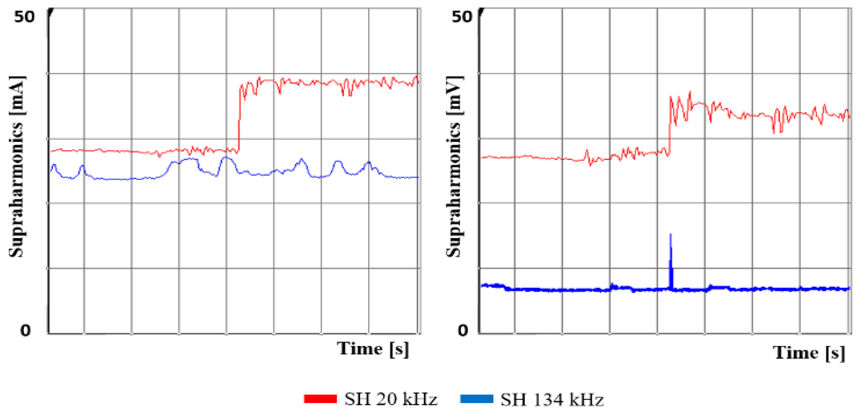
4.3.7. Influence of Grid Topology

To determine the influence of the grid topology on supraharmonic emissions, the reconstructed electrical distribution grid at the University of Applied Sciences in Vienna is operated in two different topologies—star and radial. When switching from star to radial configuration the supraharmonic current emission at the switching frequency and its first multiple increases, whereas higher supraharmonics remain stable. Figure 14 shows the supraharmonic currents in the left chart and the supraharmonic voltages in the right chart.

The amplitude of the supraharmonic current at 20 kHz increases from 30 mA (Star—village/suburban grid) to 40 mA (Radial—rural grid). The supraharmonic emission at 134 kHz remains stable at around 8 mA for both topologies. The supraharmonic voltages show similar behavior (right chart). In this case, study lower order supraharmonic emissions are more affected by grid topology type than higher order supraharmonic (>80 kHz).

4.3.8. Interpretation and Discussion

The results show that supraharmonic emissions are not necessarily increasing when operating the electric vehicle charging station at a weaker grid connection point (suburban grid versus rural grid). This emphasizes the need of individual considerations and the need of additional high-frequency grid impedance measurements.

Although the grid impedance is similar at the frequency range around 134 kHz between star and radial topology, the impedance at 20 kHz differs substantially (see Section 4.4.3). Resonance points are moved to other frequencies due to the additional inductive components caused by radial topology and the resulting longer feeder length.

4.4. Grid Impedance

In this section, the impact to the grid impedance is shown. For better visualization and interpretation, the results are separately shown for the low-frequency grid impedance (up to 2.1 kHz) and the high-frequency grid impedance (up to 150 kHz).

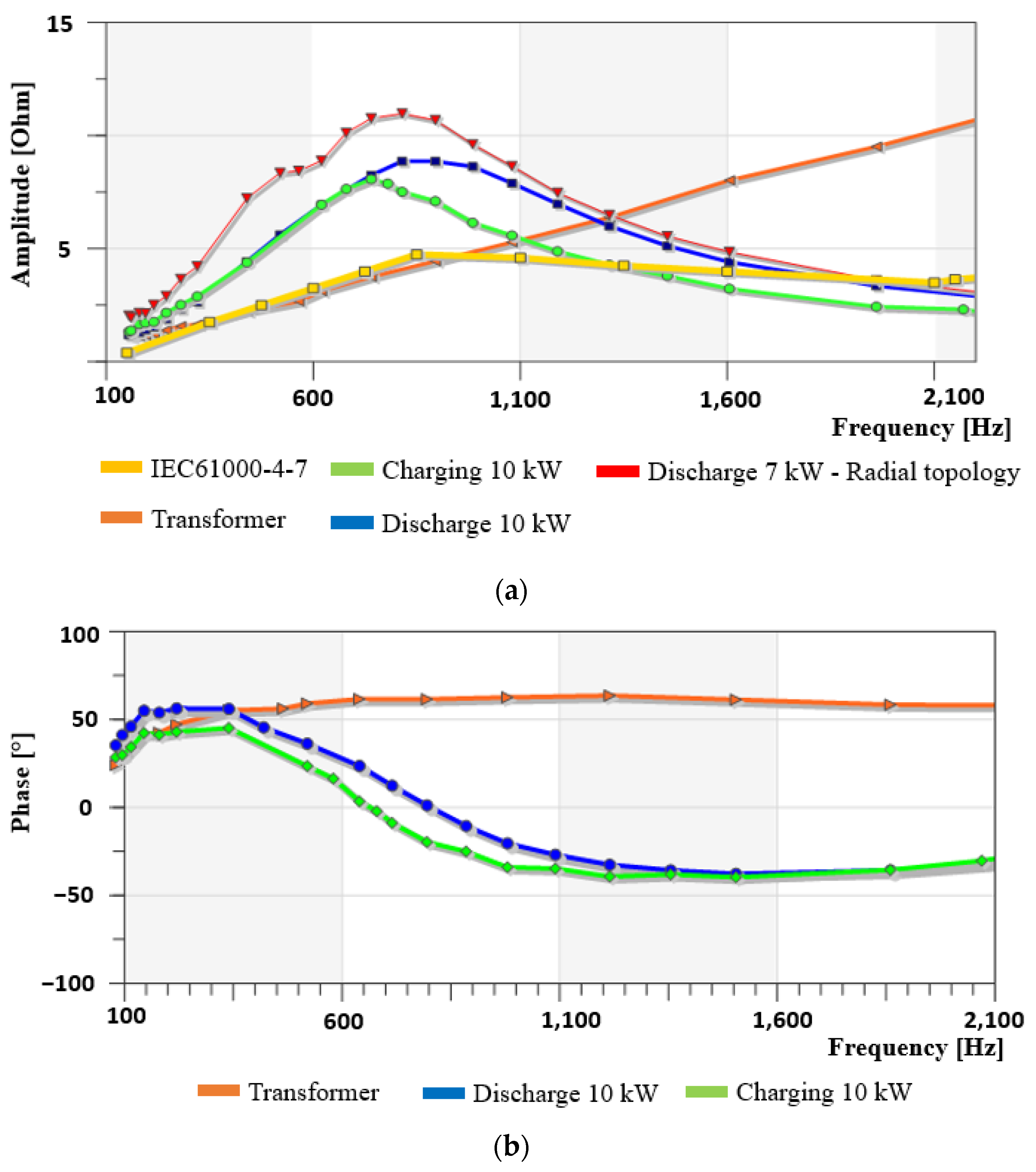
4.4.1. Grid Impedance up to 2.1 kHz

The frequency-dependent grid impedance is analyzed for charging and discharging phases as well as at the transformer station of the smart grid lab. Figure 15 shows the results of the grid impedance measurement for the amplitude (a) and the phase (b) up to 2.1 kHz:

The impedance graph at the distribution transformer station (orange) is up to 800 Hz similar to the impedance described in IEC61000-4-7 (yellow) [22] and shows ohmic-inductive behavior. The green line shows the impedance during charging and the blue line during discharging. It can be seen that the amplitudes of both are similar up to around 600 Hz and then the impedance during charging decreases by up to 2 Ω.

As soon as the charging station is connected to the electrical grid, it can be seen that the first resonance frequency of the reconstructed smart grid in the lab moved to around 700 Hz (decreased from 1600 Hz). At 650 Hz, the phase of the grid impedance will become negative and capacitive behavior is present. The red line shows the impedance when switching form star configuration (suburban/village grid) to radial configuration (rural grid) for the discharge process. In radial configuration, the grid impedance up to the 20th order increases due to higher conductor resistances and inductances. Above the 20th order, the behavior is similar for both configurations.

4.4.2. Interpretation and Discussion

The change in the grid impedance when connecting the V2G charging station is caused by the additional capacitance of the EVSE charging station introduced to the grid (LCL filter). This effect will take place even if the V2G charger is not in operation. Harmonic currents at 11th and 13th order (resulting of topology of the EVSE) are further amplified due to the lower resonance frequency, which has its peak in this frequency range.

Consequently, it is important to analyze the frequency-dependent grid impedance when analyzing harmonic emissions in the electrical grid. The latest revision of DACH-CZ regulations (EMC working group of grid operators of Germany, Austria, Switzerland and Czech Republic) considers first time the frequency-dependent grid impedance for evaluation of harmonic emissions using correction factors for certain frequencies [45]. This is especially important for evaluation at PCC where multiple electric vehicle charging stations are connected.

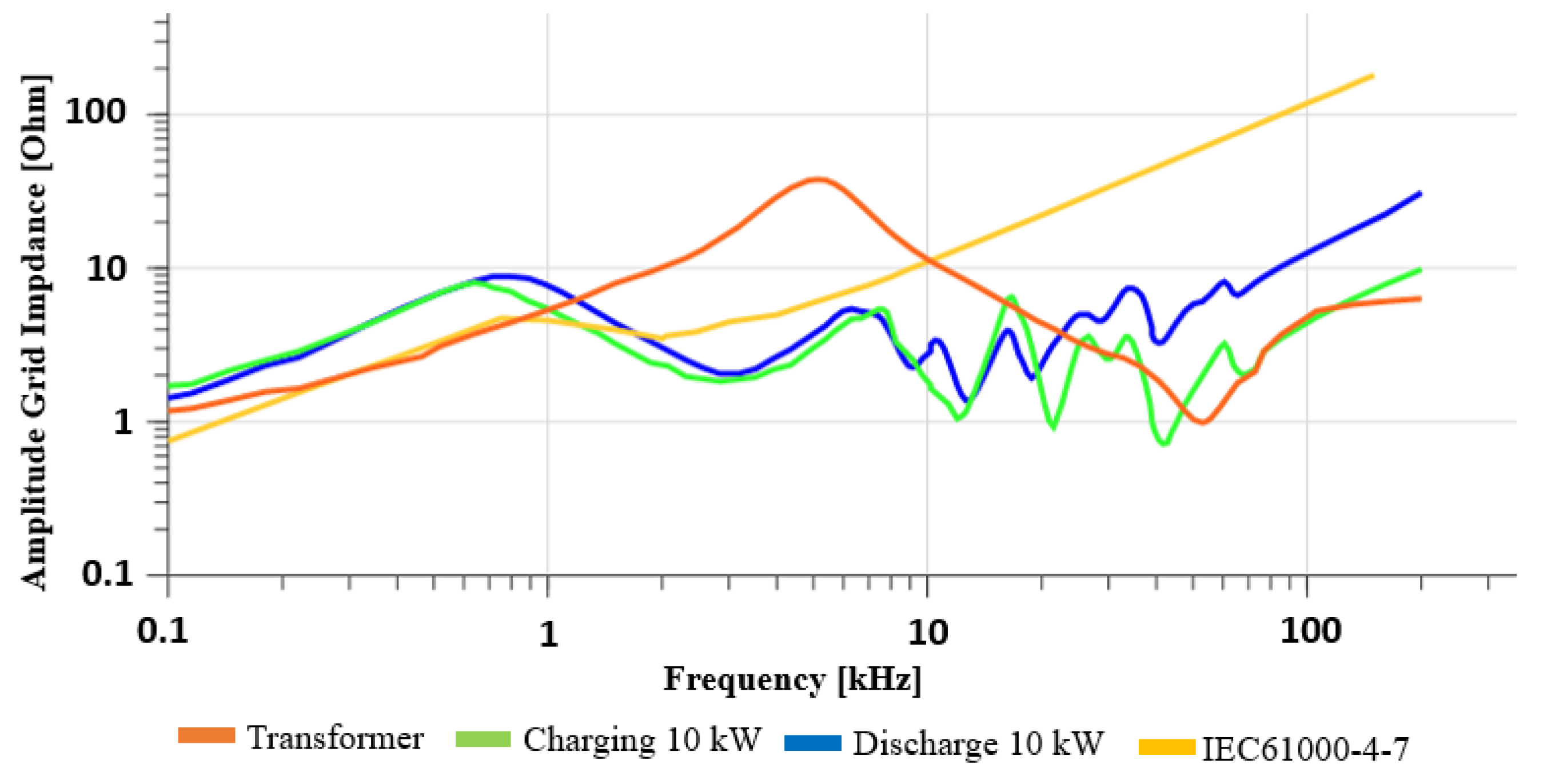
4.4.3. Grid Impedance 100 Hz–150 kHz

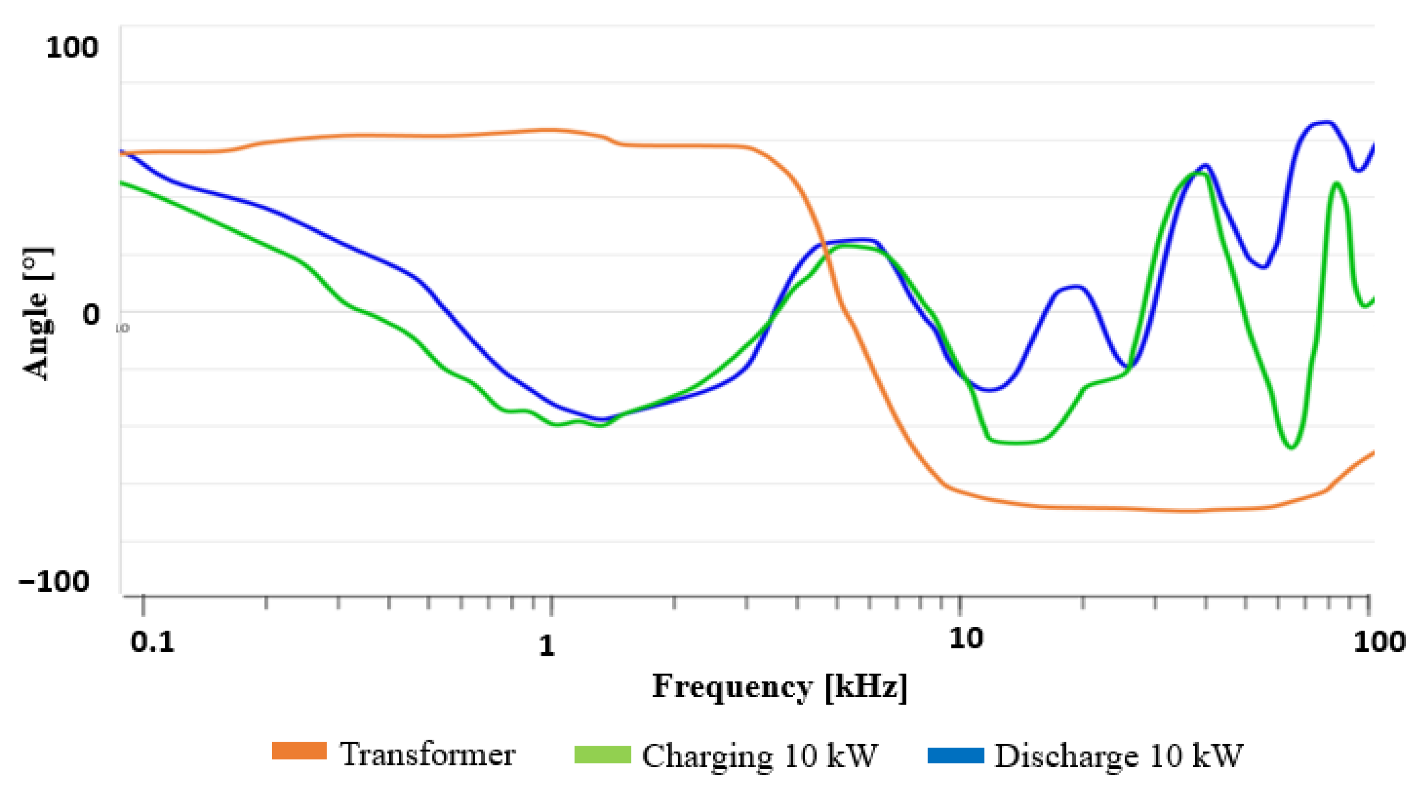
The grid impedance is measured up to 150 kHz. The simplest way to show grid characteristics is to use the impedance (respective phase) vs. frequency curve. Figure 16 shows the amplitude of the grid impedance up to 150 kHz and Figure 17 the phase angle up to 100 kHz of the transformer station (orange), during charging of the EVSE (blue), during discharging (green) and the reference impedance described in IEC61000-4-7 [22].

Although the grid impedance at the transformer station shows ohmic-inductive behavior up to 5 kHz (orange), the first resonance frequency at the PCC of the connected EVSE is around 600 Hz (blue and green), which is similar to the reference impedance described in IEC61000-4-7 (yellow) [22]. In the higher frequency range, multiple resonance points appear. The difference to the reference impedance of IEC61000-4-7 is increasing by increasing frequency. The amplitude during the discharging process is, except at one resonance point, constantly higher than during charging. Up to a frequency of 10 kHz, the difference is minor. The grid impedance in charging respective discharging mode remains the same for all power levels from 1 kW to 10 kW.

4.4.4. Interpretation and Discussion

The charts for the EVSE at the PCC for charging and discharging show that the frequency-dependent behavior is affected by the EVSE itself. The grid impedance changes between ohmic-inductive and ohmic-capacitive behavior. This change is caused by the additional capacitances of the EVSE charging station introduced to the grid. The additional capacitances of the LCL filter and the DC link causes multiple resonance points together with the ohmic-inductive grid. This is the reason for the deviation to the reference impedance of IEC61000-4-7. Consequently, these additional capacitances due to the LCL filter, the DC link capacitor, etc. need to be considered for realistic harmonic and supraharmonic emission investigations and simulation models.

Parallel resonance with high impedance values causes high harmonic voltages at this frequency if supraharmonics are emitted in this range. Series resonance with low impedance values can be the sink of supraharmonic emissions at that frequency. This gives an explanation for the results of the field test in [39]. In this study a high supraharmonic voltage at an electric vehicle charging station is measured even if there is no electric vehicle connected.

The resulting variations of the grid impedance up to 150 kHz give an answer to the findings in [41] where supraharmonics spread up to 16 km and in [10] supraharmonics stay within the installation. This emphasizes the importance of high-frequency grid impedance measurements. The results out of the field tests at different distribution transformer stations in [13] shows in general a similar behavior to the curve defined in IEC61000-4-7 [22] whereby the amplitude differs from location to location. In this study the similarity to the IEC61000-4-7 [22] curve is only given up to around 2 kHz. Above this frequency the impact of the bi-directional V2G charger is substantially influencing the frequency-dependent grid impedance. This underlines the need to consider high-power electronic devices for future simulation models and power quality assignments.

The reason for the different curves for charging (green) and discharging (blue) can be explained by the power electronics (buck vs. boost converter operation) and the type of operation (load vs. infeed).

4.5. Efficiency

To achieve reliable results, multiple charging/discharging cycles of the V2G charging station are performed. The tests are conducted at an ambient temperature of 18 °C.

Table 4. Results out of the efficiency measurements.

Power	AC to DC	DC to AC	V2G Roundtrip
7–10 kW	91.5%	96.2%	85.5%
5–7 kW	90.5%	95.1%	84.1%
2–4 kW	87.1%	93.1%	76.3%
0–2 kW	<75%	<80%	<60%

shows the measured efficiencies for AC to DC, DC to AC and V2G roundtrip operation divided by the charging/discharging power.

All values in the table are averaged results out of multiple charge/discharge operations and divided in four different power groups. The highest efficiency levels are reached at a nominal power of 10 kW of the V2G charger. The efficiency for discharging the electric vehicle (DC to AC) is always higher than for charging (DC to AC) and can reach levels of up to 96%. The lowest efficiency numbers are reached at low power levels. Charging/Discharging the vehicle with a power below 1 kW will result in a V2G roundtrip efficiency below 50%.

Interpretation and Discussion

According to [46], efficiencies for V2G chargers found in literature vary between 55% and 100%. The tests executed in [46] show an average V2G efficiency between 79% and 87%. These values are very similar to the measured efficiencies in this study. Compared with the measurements in [46] in this study the V2G roundtrip efficiency also the DC to AC and AC to DC efficiencies are determined. The determined V2G efficiencies are similar to the results in [46]. Furthermore, additional tests at low power levels down to 0.5 kW are executed. Using the V2G charging stations for household applications requires dynamic charging power levels, as an overproduction of photovoltaic systems might be used for charging of the electric vehicle.

Although the efficiency is lower at low SoC values due to higher internal resistance and higher heat generation, the overall impact of the SoC is small according to [46]. In discharge operation electric vehicles often only allow discharging to a certain SoC. In this case, the EV could be discharged till an SoC of 30%.

The investigated V2G charger is designed for operation at nominal power of 10 kW. At this operation point the efficiency for power conversion is very high and the charging-discharging losses within the vehicle battery are low. Even if the efficiency for the round-trip operation is very high at nominal power, the efficiency drops substantially at low power levels. Considering the use-case of a household application of the V2G charging station, a PV overproduction of 1 kWh charged to the EV and discharged with a power of 1 kW will result in only 0.5 kWh effective usage of the energy due to the high losses at low power levels. Consequently, for integrating a V2G charger for private or commercial purposes, the system efficiencies at different power levels need to be considered. Even if other factors such as weather and SoC are affecting the V2G roundtrip efficiency, in this study the nominal charging/discharging power is the main influence factor for the efficiency.

4.6. Reactive Power

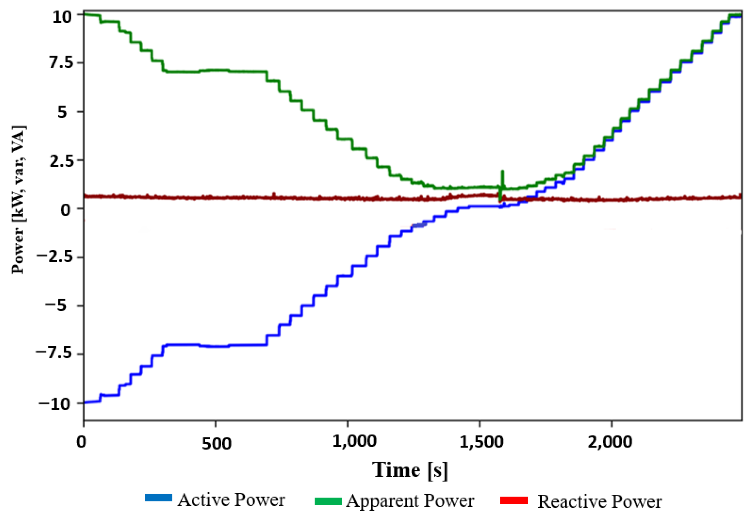
The EVSE charging station contains of an active power factor correction circuit. Figure 18 shows the active, reactive and apparent power for set points from 0 to 10 kW.

The reactive power stays almost constant (red line) for power set points from 0 to 10 kW and only increases slightly at higher power levels. Therefore, at high power levels the EVSE will operate with high power factor (PF) close to 1. However, at low power levels (<1 kW) the PF will decrease significant. When charging the EV with 1 kW, a reactive power of 1 kVA will be consumed (PF = 0.7). Below 1 kW charging/discharging power the reactive power consumption will exceed active power. Charging with 500 W will result in a power factor of 0.35. The behavior for discharge operation is similar and therefore is not shown explicitly.

Discussion

Active power factor correction of the EVSE will maintain a power factor close to 1 at high power levels (5 to 10 kW). Nevertheless, at low power levels, reactive power consumption will exceed active power levels and will cause a low power factor (0.35). The low power factor at operation with low power should be considered at private V2G applications when charging power is adjusted, e.g., depending on photovoltaic generation.

As this type of charging stations cannot support voltage controls such as PV systems, the local voltage at the PCC will increase while the EV is discharged. High penetration of this type of charging stations at the electrical grid can lead to locally too high voltage levels, similar to the problem of early PV systems.

5. Conclusions

The high-switching frequencies of modern power electronics cause harmonic and supraharmonic emissions to the electrical grid. Although emission measurements at laboratory conditions give results for idealized conditions and field tests strongly depend on local grid conditions, the real-life operation of an EVSE at a well-known reconstructed grid gives valuable information about the harmonic and supraharmonic behavior and impact to the grid impedance of a bidirectional EVSE.

Even if the EVSE fulfills all limits according to IEC61000-3-2 and IEEE519 in low-power operation and in constant voltage charging phase, the EVSE represents a major source of harmonics with a THD_i of up to 48%.

The EVSE represents a source of wide-band and narrow-band supraharmonic emissions. Narrow-band emissions occur at the switching frequency and multiples of it (PWM modulation). Wide-band emissions occur at higher frequencies (DC-DC converter) and in the case when the PTC heater is activated. Consequently, both narrow-band and wide-band emissions need to be considered in simulation models. The level of supraharmonic emissions remains stable at all power levels and therefore needs to be considered as current source for simulation and modelling. The comparison of measurement methods described in IEC61000-4-7 and IEC61000-4-30 Ed.3 (modified to gapless method) demonstrates the benefits of each grouping method and emphasizes the need of the definition of a common procedure.

The introduction of additional capacitance to the grid due to connection of the EVSE impacts the grid impedance. In this case, the first resonance frequency is moved from 1600 Hz to about 700 Hz and causes amplification of harmonics at this frequency range. Due to the amplification of harmonic currents, the emission limits at the first resonance frequency barely are met for the 11th and 13th harmonic current. In the higher-frequency range multiple resonance points appear (serial and parallel resonances) as soon as the charging station is connected to the grid (even if the EVSE is not in operation). Above 2 kHz substantial deviations of the curve defined in IEC61000-4-7 are demonstrated. The additional capacitance can represent a sink of secondary supraharmonic emissions (series resonance) as well as cause amplification of supraharmonic emissions at parallel resonance points.

Considering the use-case of a household application of the V2G charging station, a PV overproduction of 1 kWh charged to the EV and discharged with a power of 1 kW will result in only 0.5 kWh effective usage of the energy due to the high losses at low power levels. Consequently, for integrating a V2G charger for private or commercial use, the system efficiencies at different power levels need to be considered. Even if EVSE has low harmonic emissions and a high efficiency and high power-factor at nominal power, the relative harmonic emissions increase substantially at low-power operation and the efficiency can drop substantially. Finally, the EVSE does not support voltage control and can lead to locally too high voltage levels during discharge operation. Therefore, similar requirements for bidirectional EVSE as for grid-connected PV systems are needed in future regulations.