
A Control Strategy to Avoid Drop and Inrush Currents during Transient Phases in a Multi-Transmitters DIPT System

 , ,
, ,
Abstract
:1. Introduction
2. Topology of the Studied System
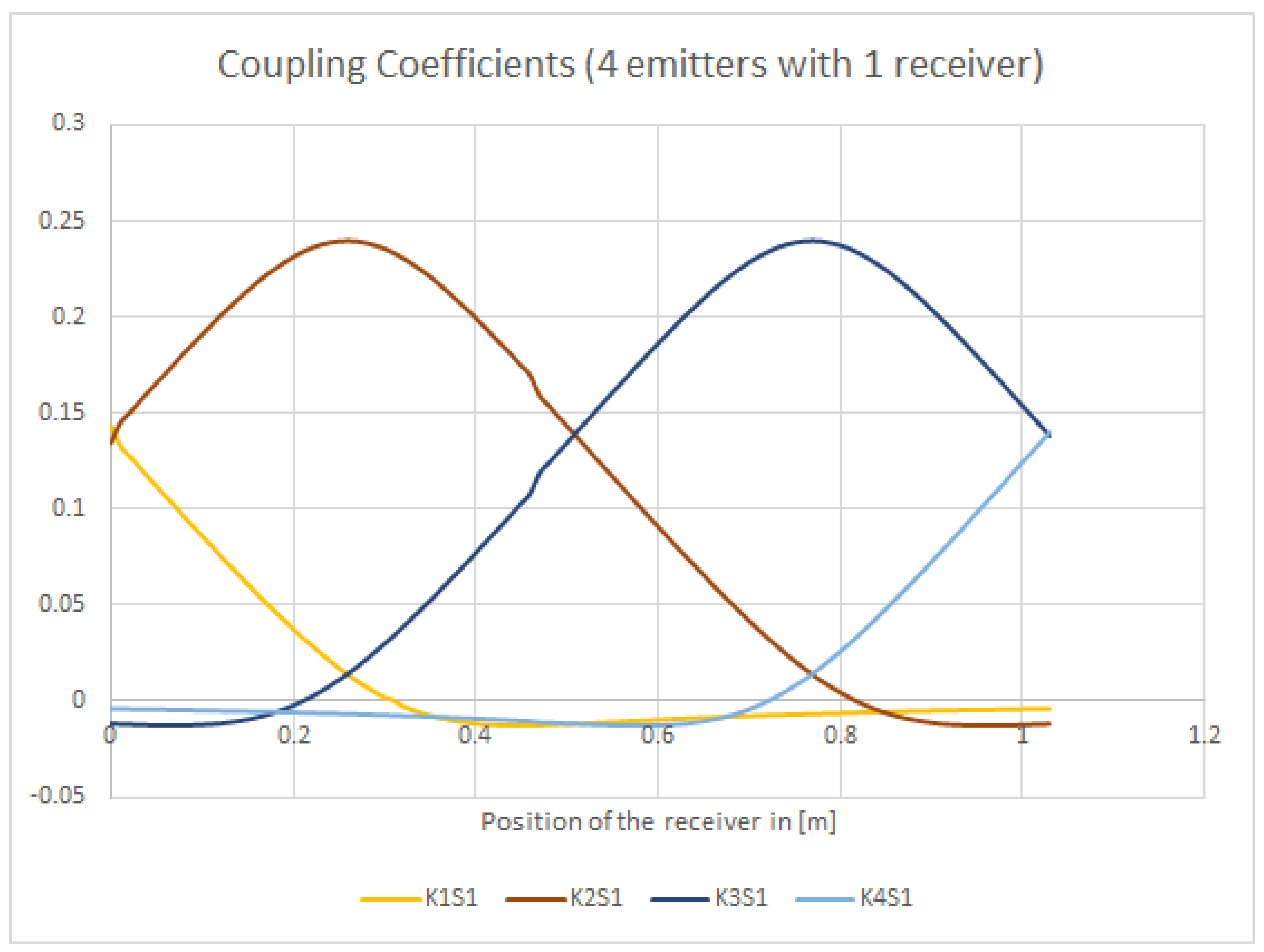
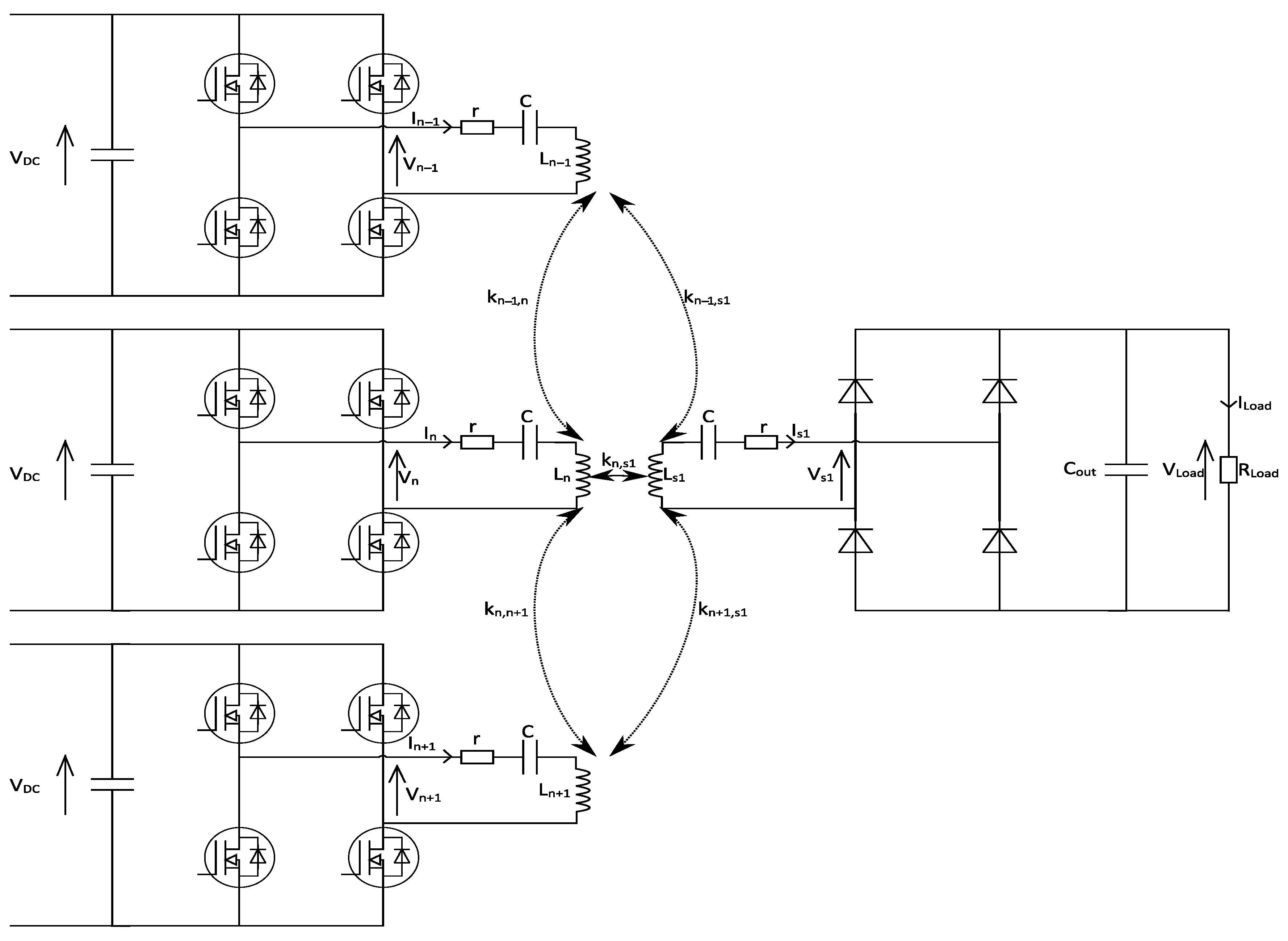
2.1. Magnetic Coupler Architecture
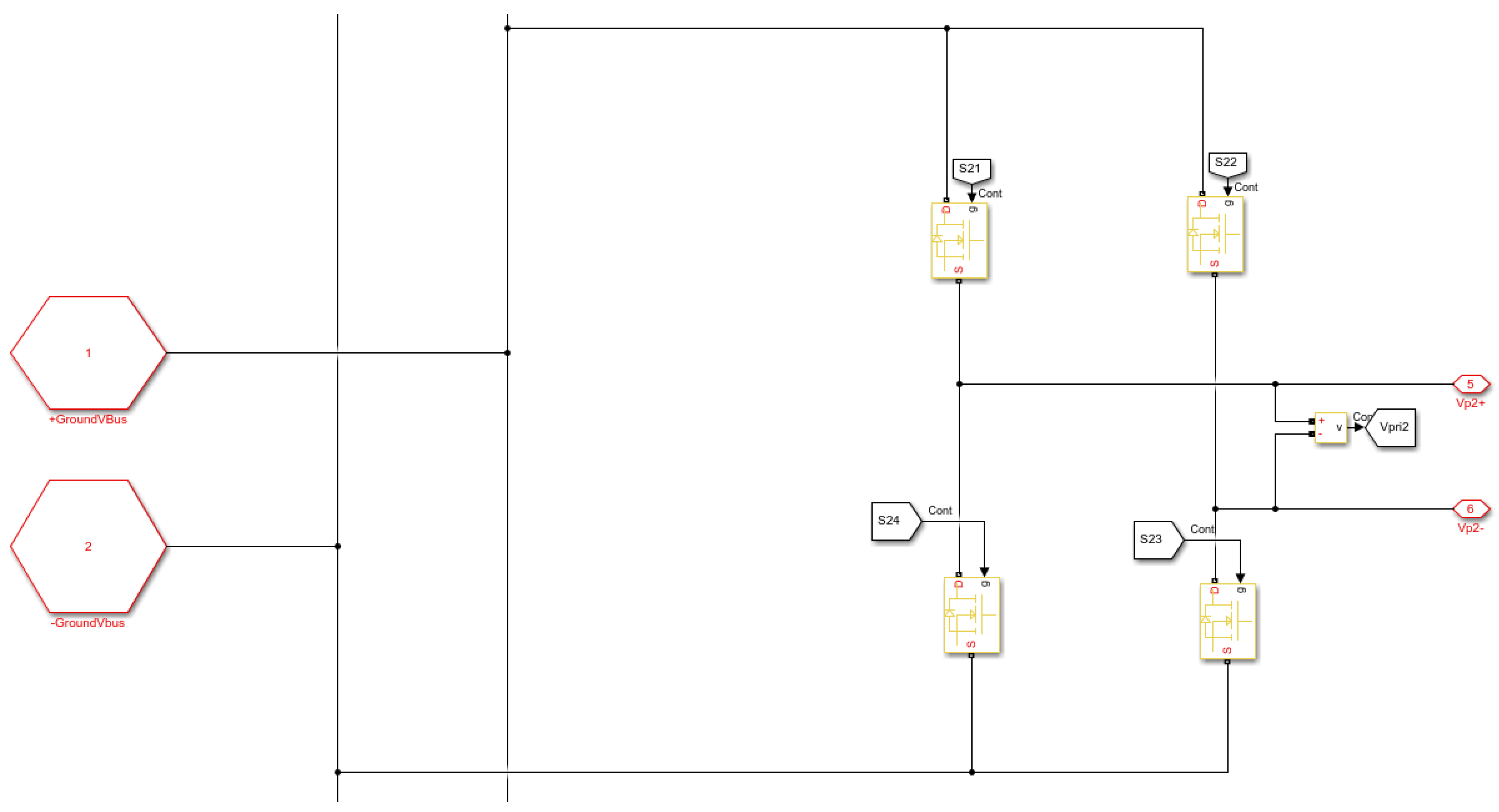
2.2. Power Electronics Architecture
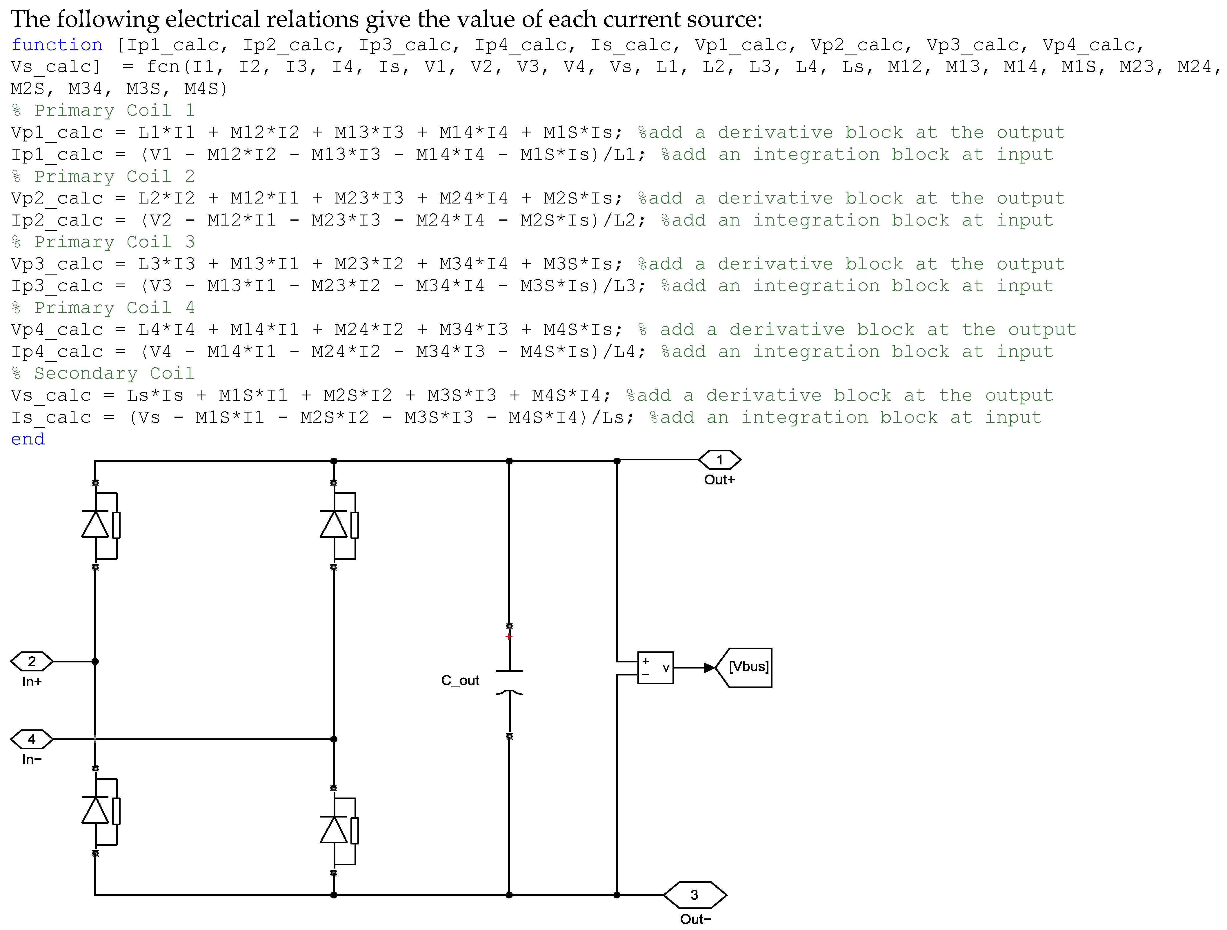
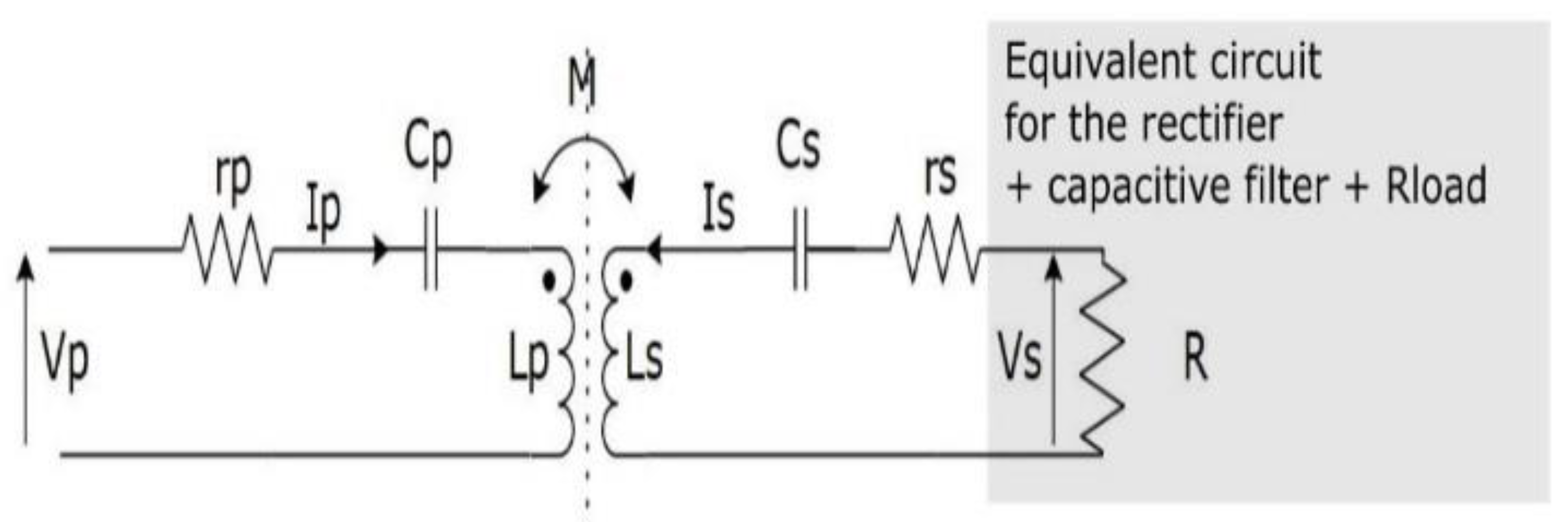
2.3. Electrical Equations of the Symmetrical Series Compensation Network
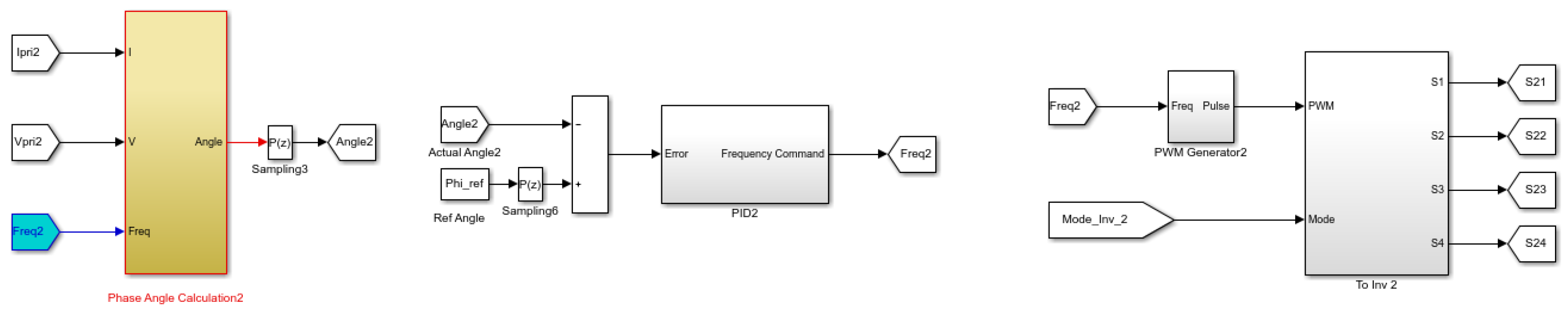
3. Control Strategy of the Transmitters’ Inverters
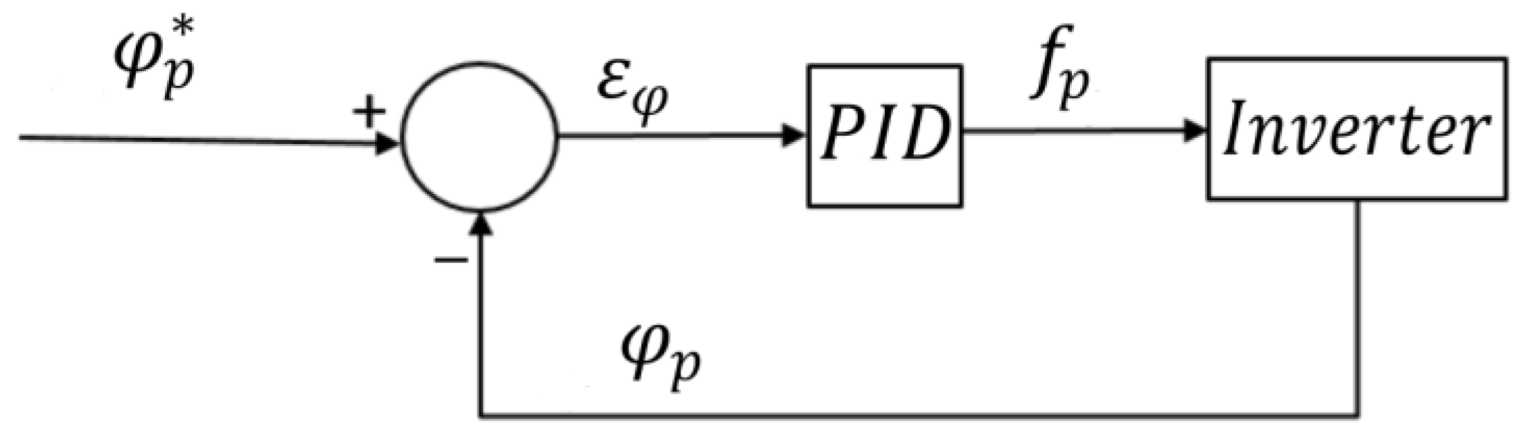
3.1. Control Loop
- 1.
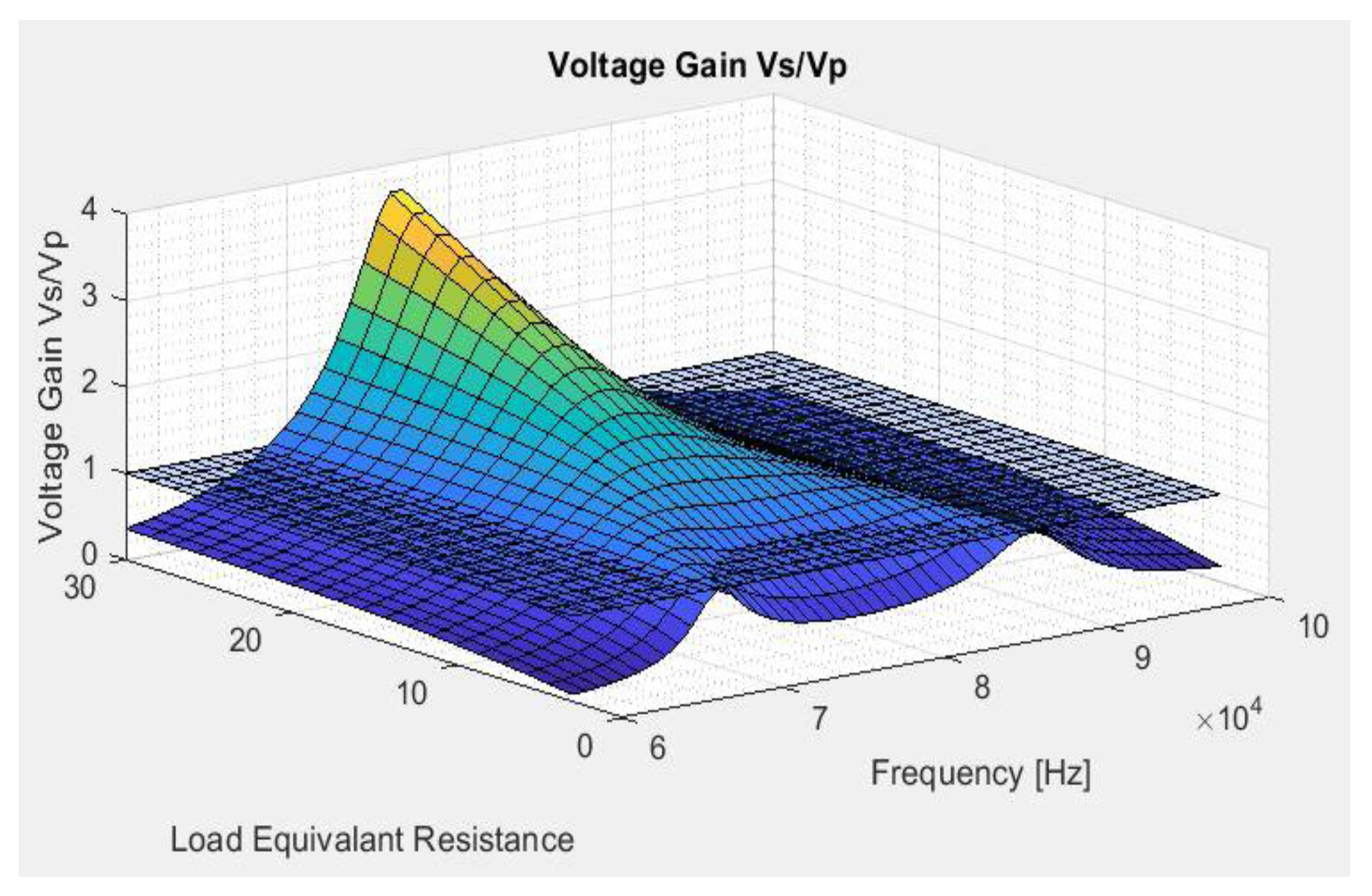
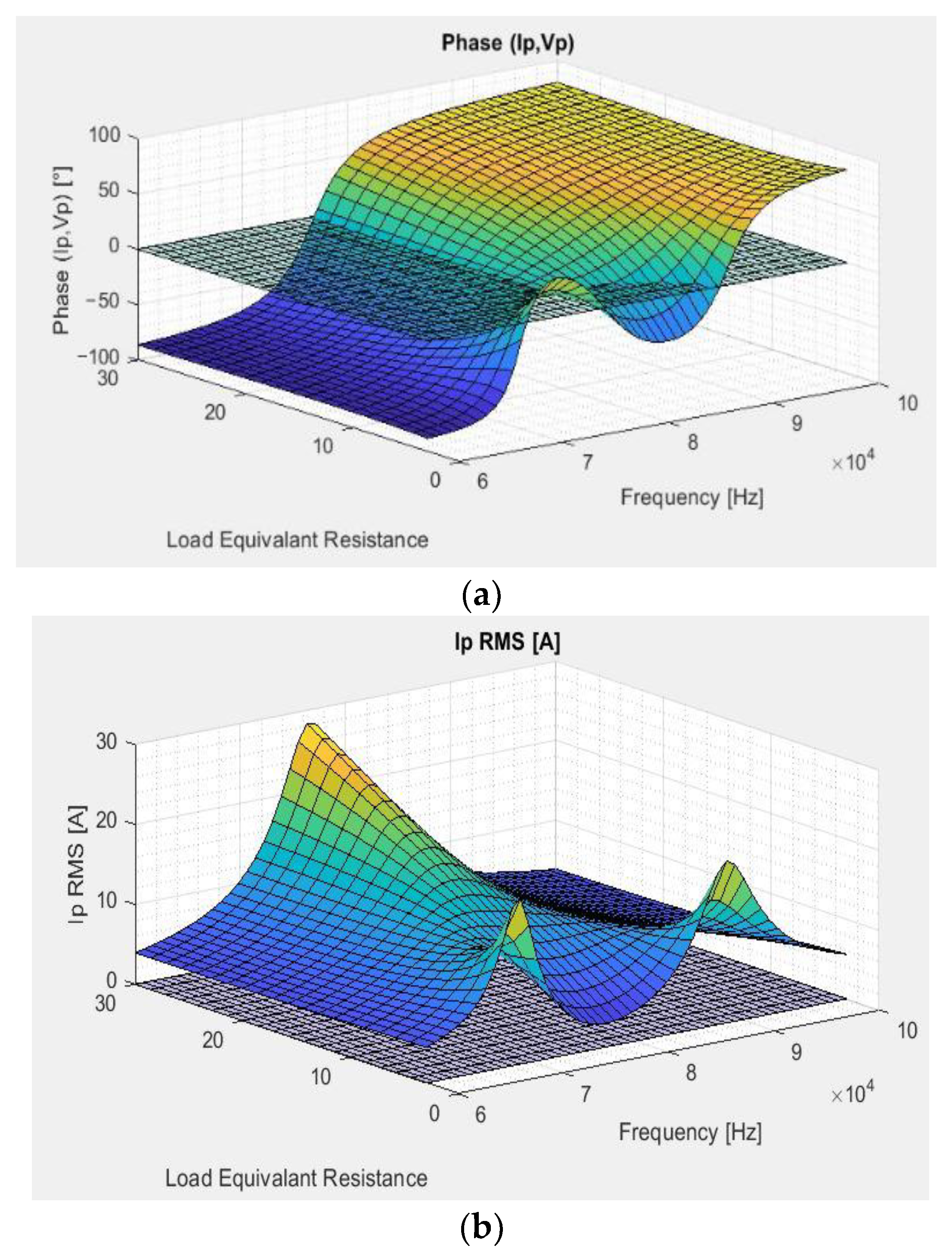
- Primary to secondary voltage gain () varies considerably with the variation of and . It reaches dangerously high levels with low power transfer;
- 2.
- Impossible to operate without the presence of the secondary system or with low coupling values since the primary coil will act as a short circuit, and a substantial current will circulate.
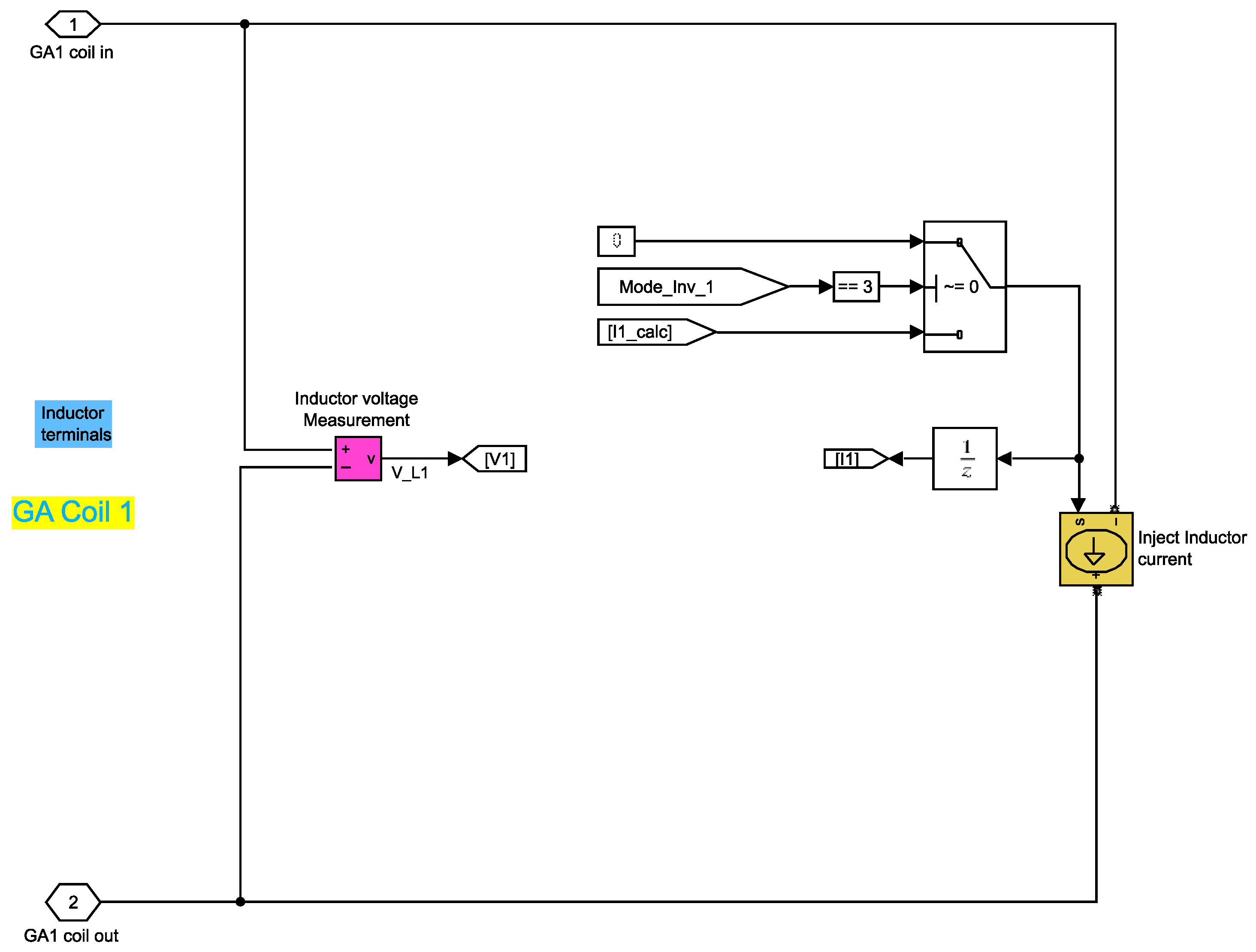
3.2. Soft-Start and Degraded Mode Integration
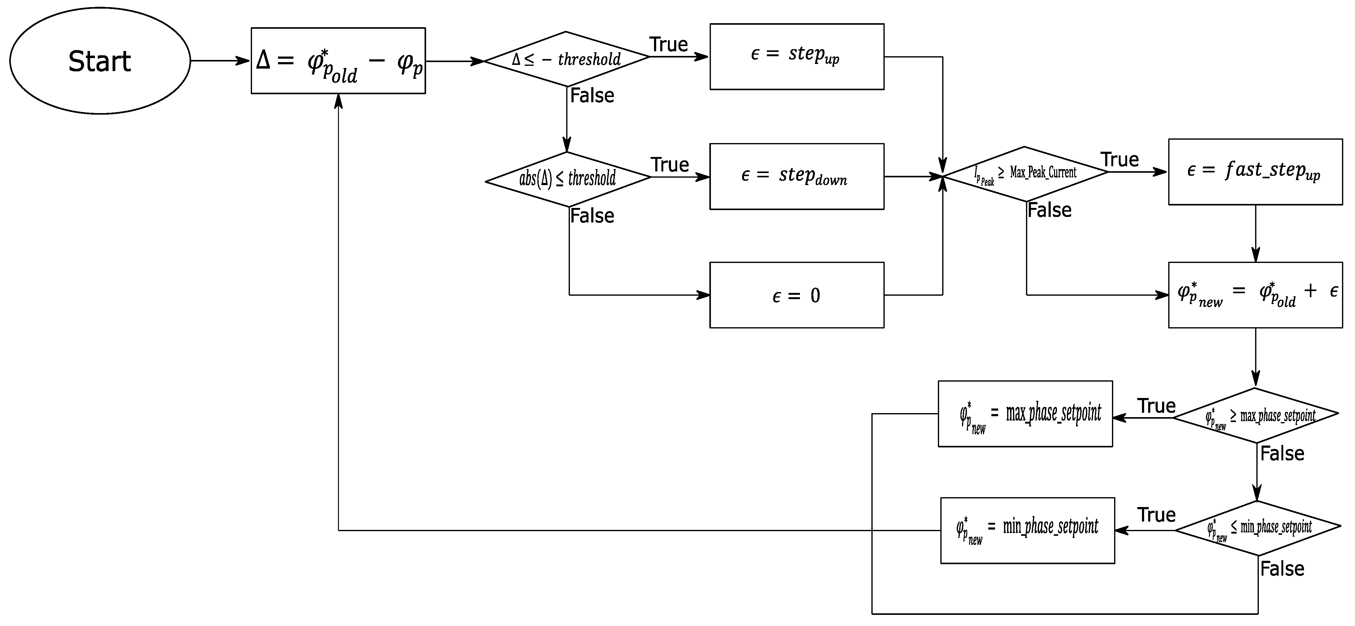
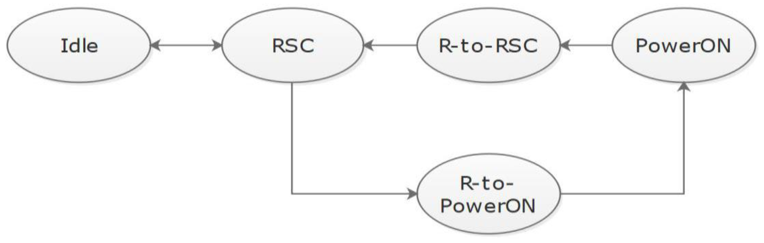
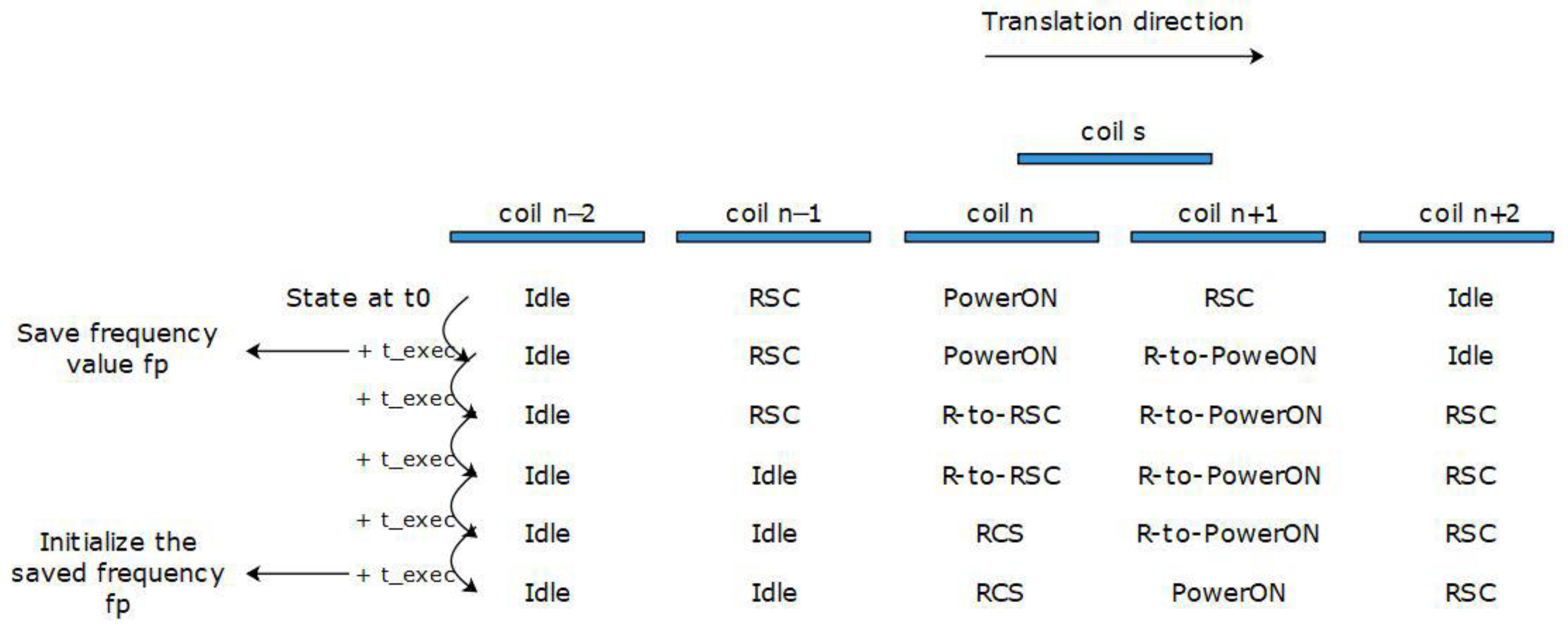
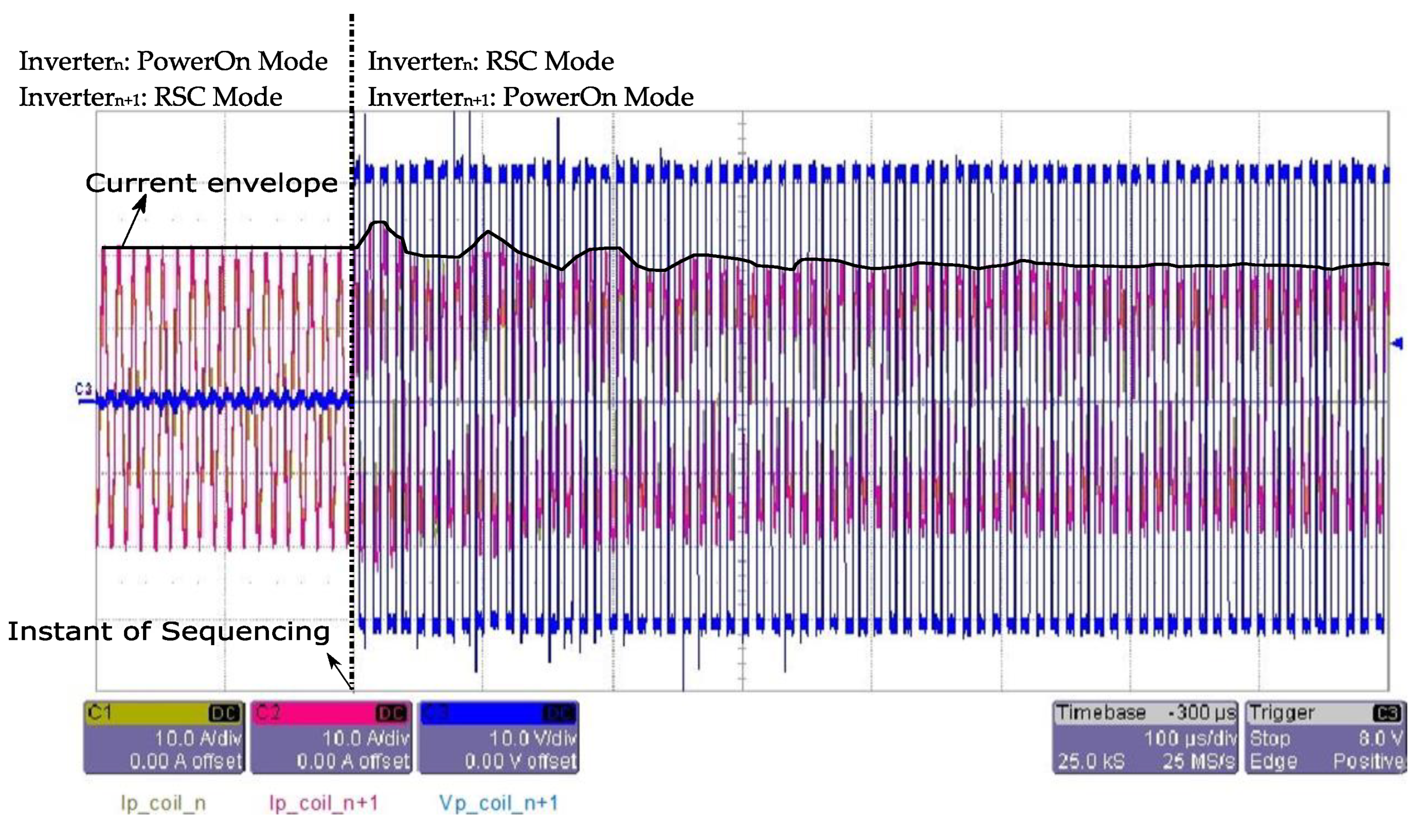
3.3. Sequencing Control
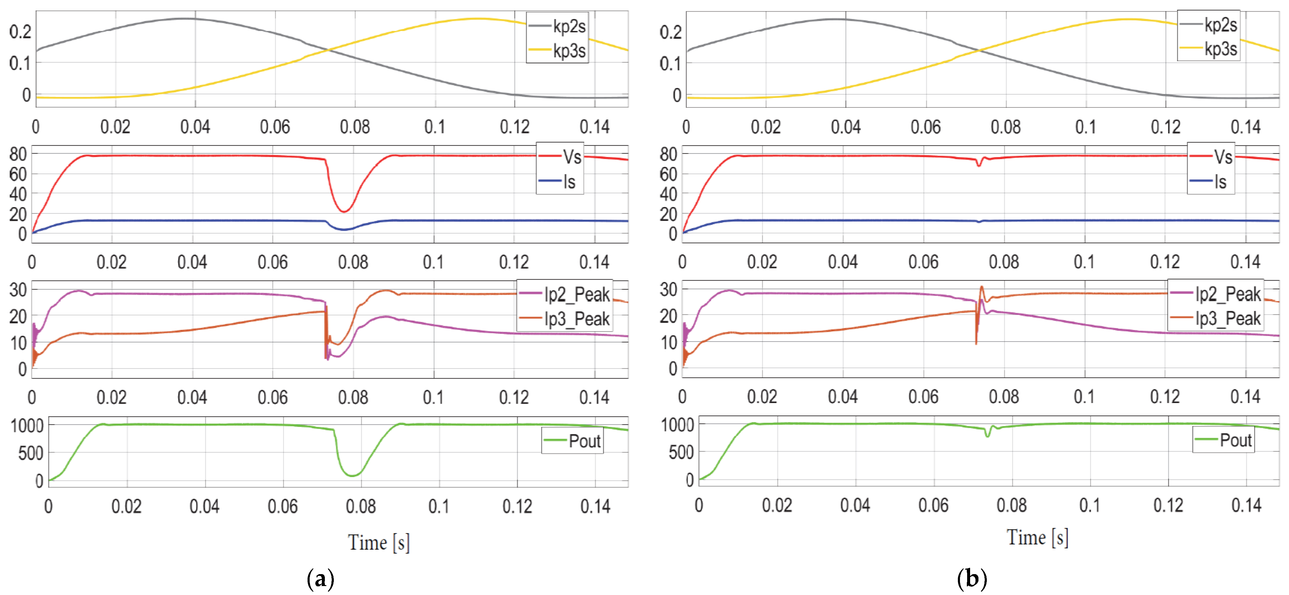
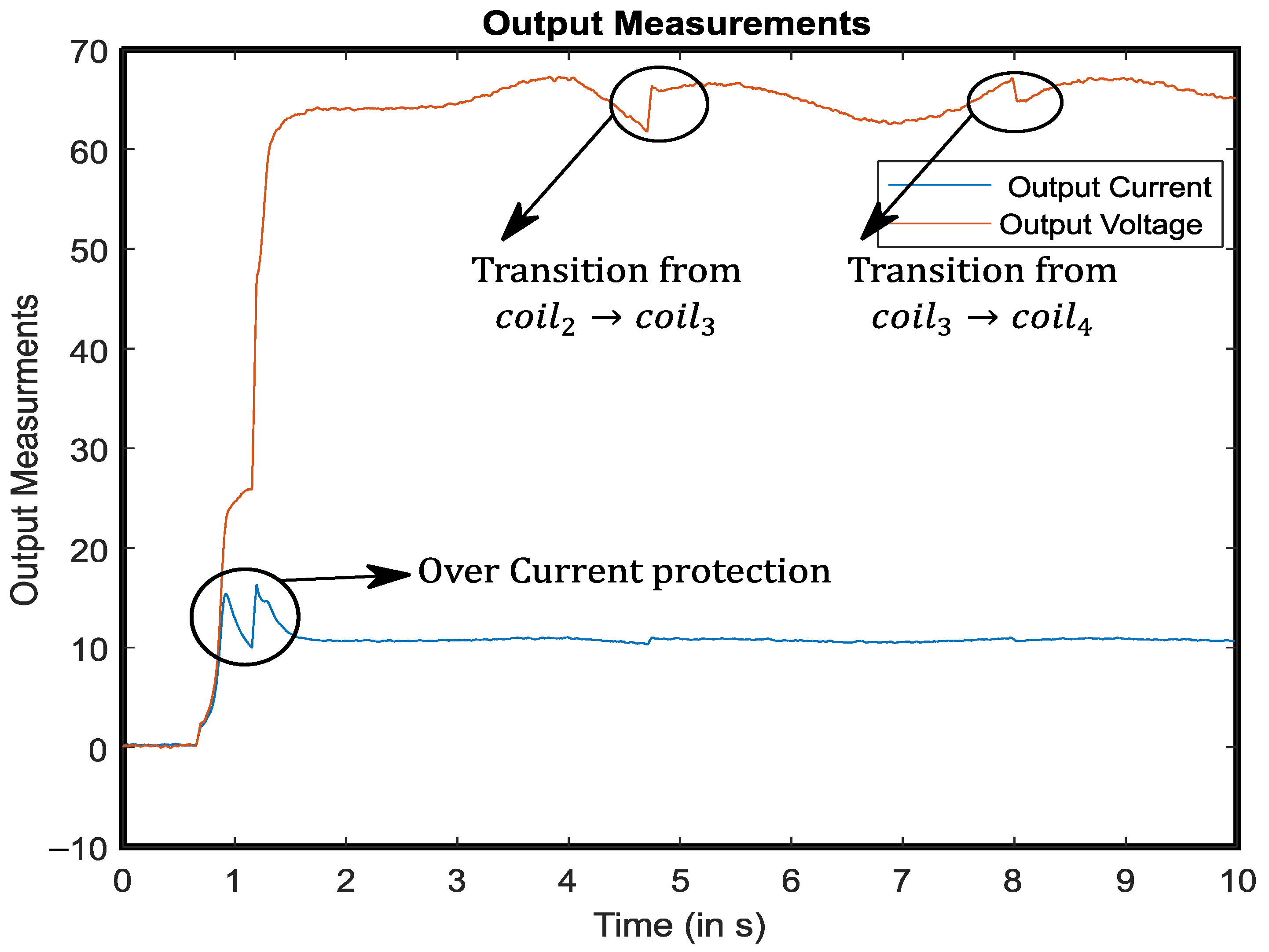
4. Simulation Results
5. Experimental Testing
6. Conclusions
Author Contributions
Funding
Institutional Review Board Statement
Informed Consent Statement
Conflicts of Interest
Appendix A


References
- Gota, S.; Huizenga, C.; Peet, K.; Medimorec, N.; Bakker, S. Decarbonising transport to achieve Paris Agreement targets. Energy Effic. 2009, 12, 363–386. [Google Scholar] [CrossRef]
- Bernard, Y.; Miller, J.; Wappelhorst, S.; Braun, C. Impacts of the Paris Low-Emission Zone and Implications for other Cities. True Real Urban Emiss. Initiat. 2020, 3–17. [Google Scholar]
- Trends and Developments in Electric Vehicle Markets—Global E.V. Outlook 2021—Analysis, IEA. Available online: https://www.iea.org/reports/global-ev-outlook-2021/trends-and-developments-in-electric-vehicle-markets (accessed on 11 April 2022).
- Panday, A.; Bansal, H.O. Green transportation: Need, technology and challenges. Int. J. Glob. Energy Issues 2004, 37, 304–318. [Google Scholar] [CrossRef]
- Züttel, A.; Remhof, A.; Borgschulte, A.; Friedrichs, O. Hydrogen: The future energy carrier. Philos. Trans. R. Soc. A Math. Phys. Eng. Sci. 2010, 368, 3329–3342. [Google Scholar] [CrossRef]
- Hydrogen Storage, Energy.gov. Available online: https://www.energy.gov/eere/fuelcells/hydrogen-storage (accessed on 1 March 2022).
- Singla, M.K.; Nijhawan, P.; Oberoi, A.S. Hydrogen fuel and fuel cell technology for cleaner future: A review. Environ. Sci. Pollut. Res. 2021, 28, 15607–15626. [Google Scholar] [CrossRef] [PubMed]
- Zhang, Z.; Pang, H.; Georgiadis, A.; Cecati, C. Wireless power transfer—An overview. IEEE Trans. Ind. Electron. 2018, 66, 1044–1058. [Google Scholar] [CrossRef]
- Hutchinson, L.; Waterson, B.; Anvari, B.; Naberezhnykh, D. Potential of wireless power transfer for dynamic charging of electric vehicles. IET Intell. Transp. Syst. 2019, 13, 3–12. [Google Scholar] [CrossRef] [Green Version]
- Duarte, G.; André, S.; Baptista, P. Assessment of wireless charging impacts based on real-world driving patterns: Case study in Lisbon, Portugal. Sustain. Cities Soc. 2021, 71, 102952. [Google Scholar] [CrossRef]
- Covic, G.A.; Boys, J.T. Modern trends in inductive power transfer for transportation applications. IEEE J. Emerg. Sel. Top. Power Electron. 2013, 1, 28–41. [Google Scholar] [CrossRef]
- Omer, C.; Onar, S.C.; Larry, S.; Cliff, W.; Madhu, C.; Lixin, T.; Paul, C.; Burak, O.; Smith, D.E. Wireless Charging of Electric Vehicles; Oak Ridge National Laboratory: Oak Ridge, TN, USA, 2016.
- Kadem, K.; Cheriet, F.; Laboure, E.; Bensetti, M.; le Bihan, Y.; Debbou, M. Sensorless Vehicle Detection for Dynamic Wireless Power Transfer. In Proceedings of the 2019 21st European Conference on Power Electronics and Applications (EPE ‘19 ECCE Europe), Genova, Italy, 3–5 September 2019; pp. 1–6. [Google Scholar] [CrossRef]
- Laporte, S.; Coquery, G.; Deniau, V.; De, B.; Hautière, N. Dynamic Wireless Power Transfer Charging Infrastructure for Future EVs: From Experimental Track to Real Circulated Roads Demonstrations. World Electr. Veh. J. 2019, 10, 84. [Google Scholar] [CrossRef] [Green Version]
- Savoye, F.P.; Venet, P.; Millet, M.; Groot, J. Impact of Periodic Current Pulses on Li-Ion Battery Performance. IEEE Trans. Ind. Electron. Inst. Electr. Electron. Eng. 2012, 59, 3481–3488. [Google Scholar] [CrossRef]
- Villa, J.L.; Sallán, J.; Llombart, A.; Sanz, J.F. Design of a high frequency inductively coupled power transfer system for electric vehicle battery charge. Appl. Energy 2009, 86, 355–363. [Google Scholar] [CrossRef]
- Lu, F.; Zhang, H.; Hofmann, H.; Mi, C.C. A dynamic charging system with reduced output power pulsation for electric vehicles. IEEE Trans. Ind. Electron. 2016, 63, 6580–6590. [Google Scholar] [CrossRef]
- Kim, K.; Choi, J.W. Influences of Magnetic Couplings in Transmitter Array of MIMO Wireless Power Transfer System. In Proceedings of the 2019 IEEE Wireless Power Transfer Conference (WPTC), London, UK, 17–21 June 2019; pp. 531–535. [Google Scholar]
- International Commission on Non-Ionizing Radiation Protection. ICNIRP guidelines for limiting exposure to time-varying electric, magnetic and electromagnetic fields (1 Hz to 100 kHz). Health Phys. 2010, 99, 818–836. [Google Scholar] [CrossRef] [PubMed]
- Boys, J.T.; Chen, C.I.; Covic, G.A. Controlling Inrush Currents in Inductively Coupled Power Systems. Int. J. Emerg. Electr. Power Syst. 2006, 5, 6. [Google Scholar] [CrossRef]
- Wang, C.S.; Covic, G.A.; Stielau, O.H. Power transfer capability and bifurcation phenomena of loosely coupled inductive power transfer systems. IEEE Trans. Ind. Electron. 2004, 51, 148–157. [Google Scholar] [CrossRef]
- Ravikiran, V.; Keshri, R.K. Comparative evaluation of S.S. and P.S. topologies for wireless charging of electrical vehicles. In Proceedings of the IECON 2017—43rd Annual Conference of the IEEE Industrial Electronics Society, Beijing, China, 29 October–1 November 2017; pp. 5324–5329. [Google Scholar]
- Zhang, W.; Mi, C.C. Compensation topologies of high-power wireless power transfer systems. IEEE Trans. Veh. Technol. 2015, 65, 4768–4778. [Google Scholar] [CrossRef]
- Liu, N.; Habetler, T.G. Design of a universal inductive charger for multiple electric vehicle models. IEEE Trans. Power Electron. 2015, 30, 6378–6390. [Google Scholar] [CrossRef]
- Caillierez, A.; Sadarnac, D.; Jaafari, A.; Loudot, S. Dynamic Inductive Charging for Electric Vehicle: Modelling and Experimental Results; PEMD: Manchester, UK, 2014. [Google Scholar]
- Gori, P.A.; Sadarnac, D.; Caillierez, A.; Loudot, S. Sensorless inductive power transfer system for electric vehicles: Strategy and control for automatic dynamic operation. In Proceedings of the EPE’17 ECCE Europe, Warsaw, Poland, 11–14 September 2017; pp. 1–10. [Google Scholar]


| Parameter | Value | Unit |
|---|---|---|
| Number of turns | 6 | turns |
| Layout | 2 layers of 3 | turns |
| Space between turns | 0 | mm |
| Space coil/ferrite | 10 | mm |
| Exterior diameter of the cable | 5 | mm |
| Total thickness (coil + ferrite) | 22 | mm |
| Cable length per coil | 10.44 + 1.5 for connections | m |
| Measured inductance (without the effect of secondary ferrite) | 45 | µH |
| Measured inductance (with the secondary placed centered above the primary) | 65 | µH |
| Air gap (center to center) | 15 | cm |
| Parameters | Definition |
|---|---|
| Vp | Voltage applied on the primary side |
| rp | Total equivalent resistance on the primary side |
| Cp | Primary series compensation capacitor |
| Lp | Inductance of the primary coil |
| M | Primary to secondary mutual inductance |
| ki,j | Magnetic coupling between coili and coilj |
| Ls | Inductance of the secondary coil |
| Cs | Secondary series compensation capacitor |
| rs | Total equivalent resistance on the secondary side |
| Vs | Voltage across the equivalent load |
| R | Equivalent circuit for the rectifier + capacitive filter + Rload |
| Cout | Output capacitance |
| State | Description |
|---|---|
| Idle | All transistors of the H-bridge are set to OFF |
| RSC | The lower transistors of the H-bridge are set to ON. This way, the ground coil is in a Resonant Short Circuit with the capacitor in series |
| PowerON | The H-bridge is controlled using the dynamic phase set point to transfer power |
| R-to-PowerON | The inverter would be in RSC mode, but ready to pass to PowerOn |
| R-to-RSC | The inverter would be in PowerON mode, but ready to pass to RSC |
| Variable | Value | Unit |
|---|---|---|
| 66 | ||
| 65 | ||
| 60 | ||
| 60 | ||
| kmax | 24 | % |
| kmin | 14 | % |
| 6 | ||
| Cout | 300 | |
| Threshold | 4 | |
| Step_down | 0.4 | |
| Step_up | 0.1 | |
| Fast_step_up | 4.5 | |
| Max_phase_stepoint | 80 | |
| Min_phase_stepoint | 1 | ° |
| ) | 15 (66) | |
| 0.01 | Proportional parameter in parallel form | |
| 350 | Integrator parameter in parallel form | |
| D | Derivative parameter in parallel form | |
| 100 | ||
| 82 | ||
| 100 | ||
| 25 | km/h |
Publisher’s Note: MDPI stays neutral with regard to jurisdictional claims in published maps and institutional affiliations. |
© 2022 by the authors. Licensee MDPI, Basel, Switzerland. This article is an open access article distributed under the terms and conditions of the Creative Commons Attribution (CC BY) license (https://creativecommons.org/licenses/by/4.0/).
Share and Cite
Kabbara, W.; Bensetti, M.; Phulpin, T.; Caillierez, A.; Loudot, S.; Sadarnac, D. A Control Strategy to Avoid Drop and Inrush Currents during Transient Phases in a Multi-Transmitters DIPT System. Energies 2022, 15, 2911. https://doi.org/10.3390/en15082911
Kabbara W, Bensetti M, Phulpin T, Caillierez A, Loudot S, Sadarnac D. A Control Strategy to Avoid Drop and Inrush Currents during Transient Phases in a Multi-Transmitters DIPT System. Energies. 2022; 15(8):2911. https://doi.org/10.3390/en15082911
Chicago/Turabian StyleKabbara, Wassim, Mohamed Bensetti, Tanguy Phulpin, Antoine Caillierez, Serge Loudot, and Daniel Sadarnac. 2022. "A Control Strategy to Avoid Drop and Inrush Currents during Transient Phases in a Multi-Transmitters DIPT System" Energies 15, no. 8: 2911. https://doi.org/10.3390/en15082911
APA StyleKabbara, W., Bensetti, M., Phulpin, T., Caillierez, A., Loudot, S., & Sadarnac, D. (2022). A Control Strategy to Avoid Drop and Inrush Currents during Transient Phases in a Multi-Transmitters DIPT System. Energies, 15(8), 2911. https://doi.org/10.3390/en15082911