An Improved Approach to Calculate Eddy Current Loss in Soft Magnetic Materials Based on Measured Hysteresis Loops

Abstract

The paper presents a study of the influence of magnetic hysteresis on macroscopic eddy current losses. Usually, this loss is calculated within many simplifying assumptions, of which the most striking is not only neglecting the hysteresis, but also the nonlinearity of the material. To check how such simplifications affect the results, the loss was calculated taking into account the hysteresis phenomenon for several materials. For this purpose, an algorithm for solving Maxwell’s equations with magnetic characteristics given as a family of measured hysteresis loops was constructed. A new method for conversion between H and B fields using the measured hysteresis loops was also proposed. The results of calculations for three materials show that the eddy current loss calculated with magnetic hysteresis taken into account are smaller than those calculated via the classical formula obtained for linear materials. For the tested materials, the differences reach up to around 30%, depending on frequency, magnetic flux density and thickness of electrical sheet. This may result, among others, in erroneous determination of the excess loss in Bertotti’s approach.

1. Introduction

Energy loss is one of the most significant parameters characterizing soft magnetic materials, which is usually given per mass unit and one magnetizing cycle. In the classical approach, resulting from the Poynting theorem, there are two components of the loss: due to hysteresis and macroscopic eddy currents, respectively [1,2]. However, the loss calculated in such a way is lower compared to the measured one [3]. The difference between the measured and theoretical loss is called the excess loss. Its origin is often explained with Bertotti’s theory, also known as loss separation, where the excess loss is related with the domain structure of magnetic material [2,4,5,6,7,8,9]. Bertotti’s approach is still a field of extensive research, including its validation for new types of soft magnetic materials as well as for non-sinusoidal excitations [10,11,12,13]. However, it should be remembered that the classical formulas do not take into consideration the dynamics of domain structure (movement of domain walls, creation and annihilation of domains), i.e., they neglect the microscopic eddy currents caused by magnetic flux changes near domain walls. But there is another factor affecting this difference—it may originate (at least partially) in many simplifying assumptions used during derivation of the theoretical formulas. Among them, the most striking is using constant value for magnetic permeability in the eddy current loss, i.e., neglecting not only the magnetic hysteresis, but also the nonlinearity of magnetic material. Moreover, Bertotti uses the low frequency approximations for the hysteresis and eddy current loss, i.e., the excess loss is determined without the skin effect taken into account [14,15,16,17], which may lead to significant errors for higher frequency or thicker electric sheets. Therefore, it seems reasonable to verify how these simplifications affect the classical eddy current loss, and, thus, the excess loss [18].

There have been numerous attempts at including magnetic hysteresis into calculations of fields and eddy current loss, e.g., [19,20,21,22]. Solving the field equations with measured magnetization characteristics taken into account (hysteresis loop family or nonlinear B(H) curves) usually requires a numerical approach. An iterative algorithm, including nonlinear magnetization curve B(H), i.e., variable magnetic permeability, was presented in [23]. The algorithm was modified to incorporate the magnetic hysteresis, and its idea was presented in [24]. It was tested on various materials and for various parameters of time-spatial discretization. When the slope of hysteresis loops, dB/dH, was finite and the skin depth was small enough, the algorithm was convergent. The classical eddy current loss calculated via the algorithm was up to around 2% smaller compared to the classical theoretical value for a 6.5% Si non-oriented electric sheet of thickness 0.1 mm and frequency up to 400 Hz. Such a rather small value was due to very weak skin effect. A stronger skin effect was expected to affect the loss more significantly, but tests for thicker sheets or higher frequencies led to some problems with convergence of the algorithm. Therefore, some improvements reducing the numerical noise arising during calculations were proposed in [25]. The reduction consisted of applying Fourier transform and cutting off the higher order harmonics of amplitude lower than a prescribed percentage of the highest one. This significantly improved the convergence, but there were still problems with hysteresis loops of infinite dB/dH values. Therefore, this paper is focused on a new method of conversion between H and B fields to improve the convergence.

2. Methodology

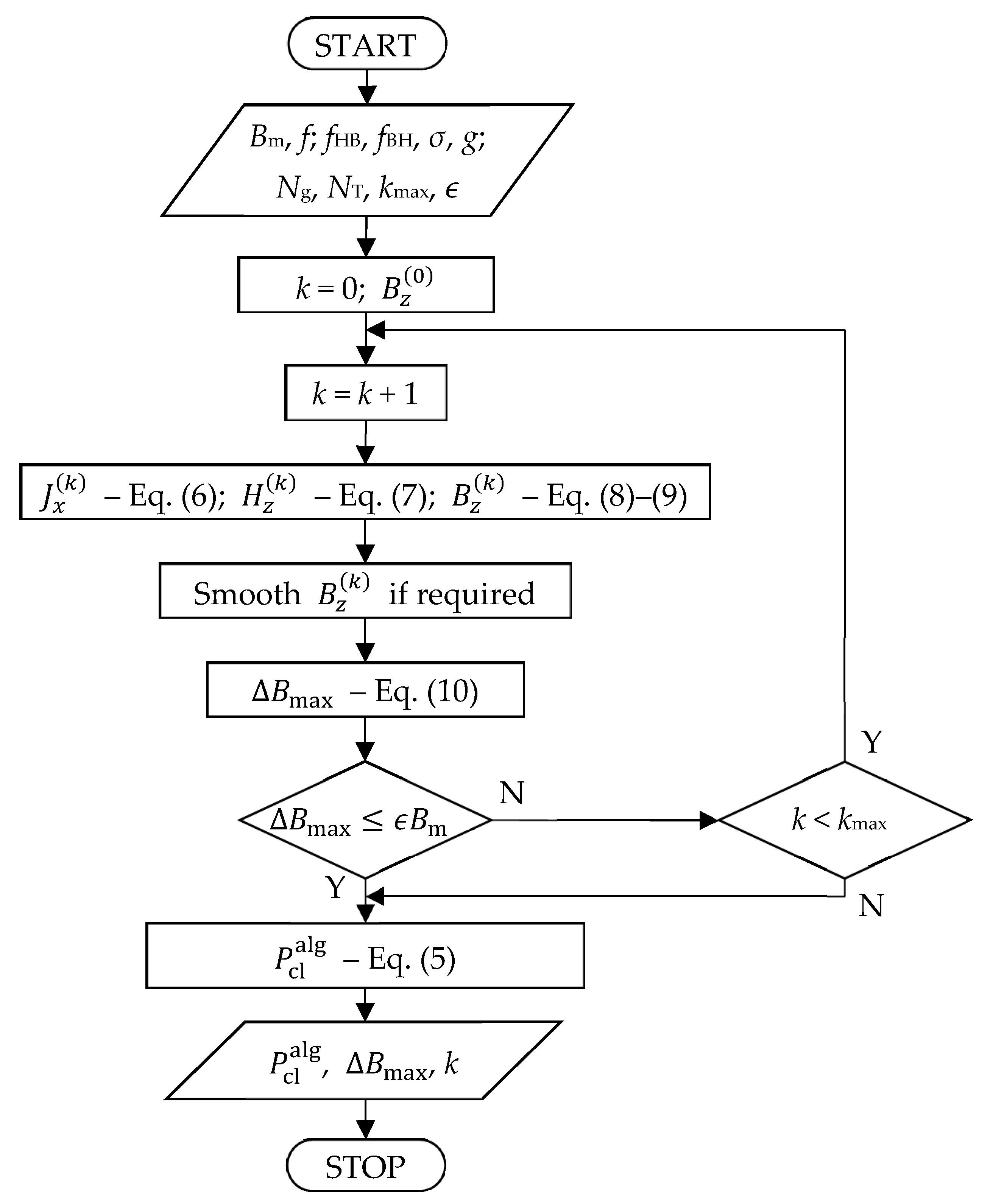
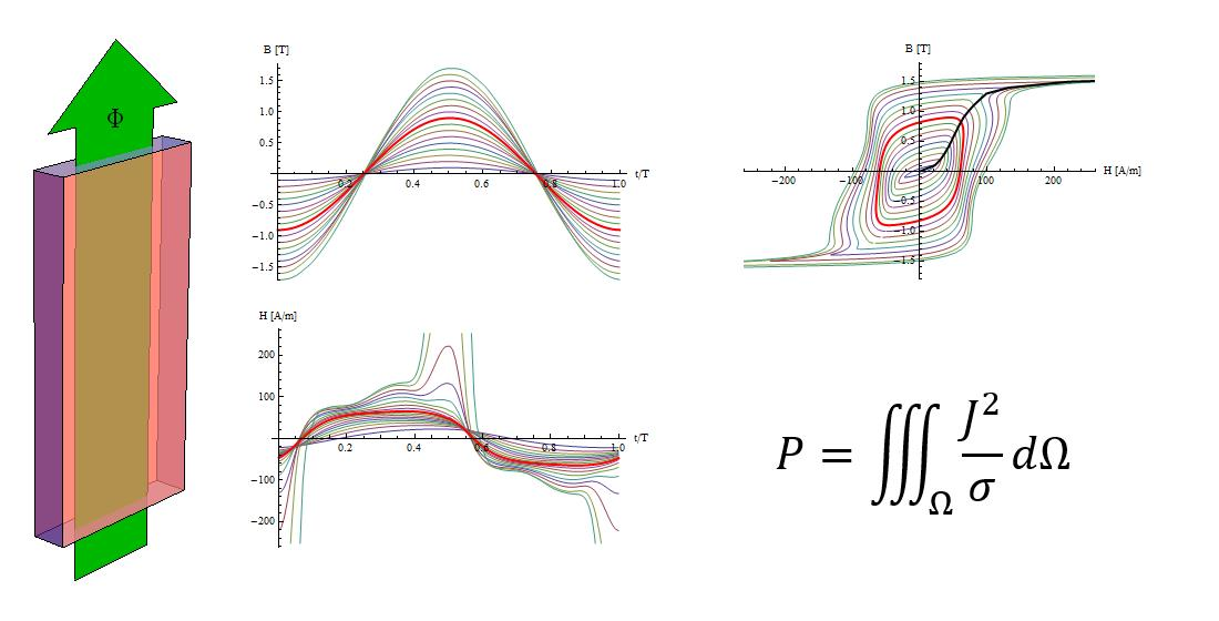
2.1. Theoretical Background: Governing Equations and Their Solving

To calculate the eddy current loss in a material sample, it is necessary to make several assumptions on geometry and material properties of the sample. Below, a rectangular sample of thickness $g$, much smaller than the other dimensions (w and l), is considered—see Figure 1. The material is assumed to be isotropic and homogeneous, with constant electric conductivity σ, and known magnetic characteristics, which may be given in the form of a hysteresis loop family or magnetization curve. Formally, the B(H) characteristics can be expressed in the following form:

$$B=f_{\mathrm{HB}}\left(H\right), H=f_{\mathrm{BH}}\left(B\right),$$

(1)

where $f_{\mathrm{HB}}$ and $f_{\mathrm{BH}}$ are mutually inverse transformations describing the magnetization curve or hysteresis loop family. The family of measured magnetic hysteresis loops for various frequencies is used here, but the same algorithm is applied for magnetization curve, or just constant magnetic permeability. After introducing the Cartesian coordinates with origin at the sample center and axes oriented as in Figure 1, and assuming the B field only has a z component depending on y, the Maxwell equations simplify as follows:

$$\frac{\partial J_x\left(y,t\right)}{\partial y}=\sigma \frac{\partial B_z\left(y,t\right)}{\partial t},$$

(2)

$$\frac{\partial H_z\left(y,t\right)}{\partial y}=J_x\left(y,t\right).$$

(3)

The above equations are solved under condition that the average magnetic flux is sinusoidal with angular frequency of ω:

$$B_{\mathrm{av}}\left(t\right)=\frac{\mathsf{\Phi }\left(t\right)}{gw}=B_{\mathrm{m}}\sin \omega t,$$

(4)

After solving the equations, the eddy currents loss is calculated as follows:

$$P_{\mathrm{cl}}^{\mathrm{alg}}=\frac{4f}{\sigma g}{{\displaystyle \int }}_{t=0}^{\frac{1}{2f}}{{\displaystyle \int }}_{y=0}^{\frac{g}{2}}{J}_x^2\left(y,t\right)\mathrm{d}y\mathrm{d}t \left[\frac{\mathrm{W}}{{\mathrm{m}}^3}\right],$$

(5)

where f is frequency.

Equations (1)–(4) are solved numerically. The block diagram of the iterative algorithm is presented in Figure 2. Suppose an approximate waveform distribution of magnetic flux density throughout the sample in iteration k−1, B^(k–1)(y, t), is known. Then Equation (2) together with symmetry condition J_x(–y, t) = −J_x(y, t) yields:

$$J_x^{\left(k\right)}\left(y,t\right)=\sigma {{\displaystyle \int }}_0^y\frac{\partial B_z^{\left(k-1\right)}\left(y,t\right)}{\partial t}\mathrm{d}y.$$

(6)

Next, Equation (3) leads to:

$$H_z^{\left(k\right)}\left(y,t\right)=\underset{{\tilde{H}}_z^{\left(k\right)}\left(y,t\right)}{\underbrace{{{\displaystyle \int }}_0^y{J}_x^{\left(k\right)}\left(y,t\right)\mathrm{d}y}}+H_{z0}^{\left(k\right)}\left(t\right),$$

(7)

where $H_{z0}^{\left(k\right)}\left(t\right)$ is any function of time. Its determination is discussed later in this section. Having found $H_z^{\left(k\right)}\left(y,t\right)$, the first of Equation (1) is used to obtain the magnetic flux density waveform corresponding to $H_z^{\left(k\right)}\left(y,t\right)$:

$${\tilde{B}}_z^{\left(k\right)}\left(y,t\right)=f_{\mathrm{HB}}\left[H_z^{\left(k\right)}\left(y,t\right)\right].$$

(8)

The tilde over $B_z$ is used here to indicate that the magnetic flux density obtained in such a way usually does not satisfy Equation (4). Therefore, the values of B field are adjusted as follows:

$$B_z^{\left(k\right)}\left(y,t\right)={\tilde{B}}_z^{\left(k\right)}\left(y,t\right)-\frac{2}{g}{{\displaystyle \int }}_0^{\frac{g}{2}}{\tilde{B}}_z^{\left(k\right)}\left(y,t\right)\mathrm{d}y+B_{\mathrm{av}}\left(t\right).$$

(9)

The adjustment subtracts the actual average magnetic flux density (the integral) and adds the required average value given by Equation (4). Note that this does not change the spatial distribution of magnetic flux density—for all $y$ coordinates, the same shift in values is performed. Hence, the derivative with respect to $y$ is not affected. Then, the difference between $B_z^{\left(k\right)}$ and $B_z^{\left(k-1\right)}$ is determined by calculating:

$$\mathsf{\Delta }{B}_{\max }=\underset{y,t}{\max }\left|B_z^{\left(k\right)}\left(y,t\right)-B_z^{\left(k-1\right)}\left(y,t\right)\right|.$$

(10)

If ΔB_max ≤ ϵB_m, where ϵ is a presumed maximum relative error, the calculations are finished, otherwise they are repeated. The other condition for finishing iterations is reaching the maximum permissible number of iterations.

Function $H_{z0}^{\left(k\right)}\left(t\right)$ occurring in Equation (7) may be assumed in various ways. Initially, it was just the value from previous iterations similarly as indicated in [23], but it led to problems with convergence. Therefore, it is proposed to determine it so that the average H field throughout the sample was:

$$H_{\mathrm{av}}\left(t\right)=f_{\mathrm{BH}}\left[B_{\mathrm{av}}\left(t\right)\right],$$

(11)

which is known, because B_av(t) is given by Equation (4) and f_BH is a known characteristic. Calculating the average value from Equation (7) and comparing it with Equation (11) yields:

$$H_{z0}^{\left(k\right)}\left(t\right)=H_{\mathrm{av}}\left(t\right)-\frac{2}{g}{{\displaystyle \int }}_0^{\frac{g}{2}}{\tilde{H}}_z^{\left(k\right)}\left(k,t\right)\mathrm{d}y.$$

(12)

This allowed much better convergence to be obtained.

In numerical implementation, the half-period was divided into N_T time segments of equal duration Δt = T/(2N_T), and half the thickness of the sheet was divided into N_g segments of equal length Δy = g/(2N_g). The derivatives and integrals were replaced with appropriate finite differences and sums, respectively.

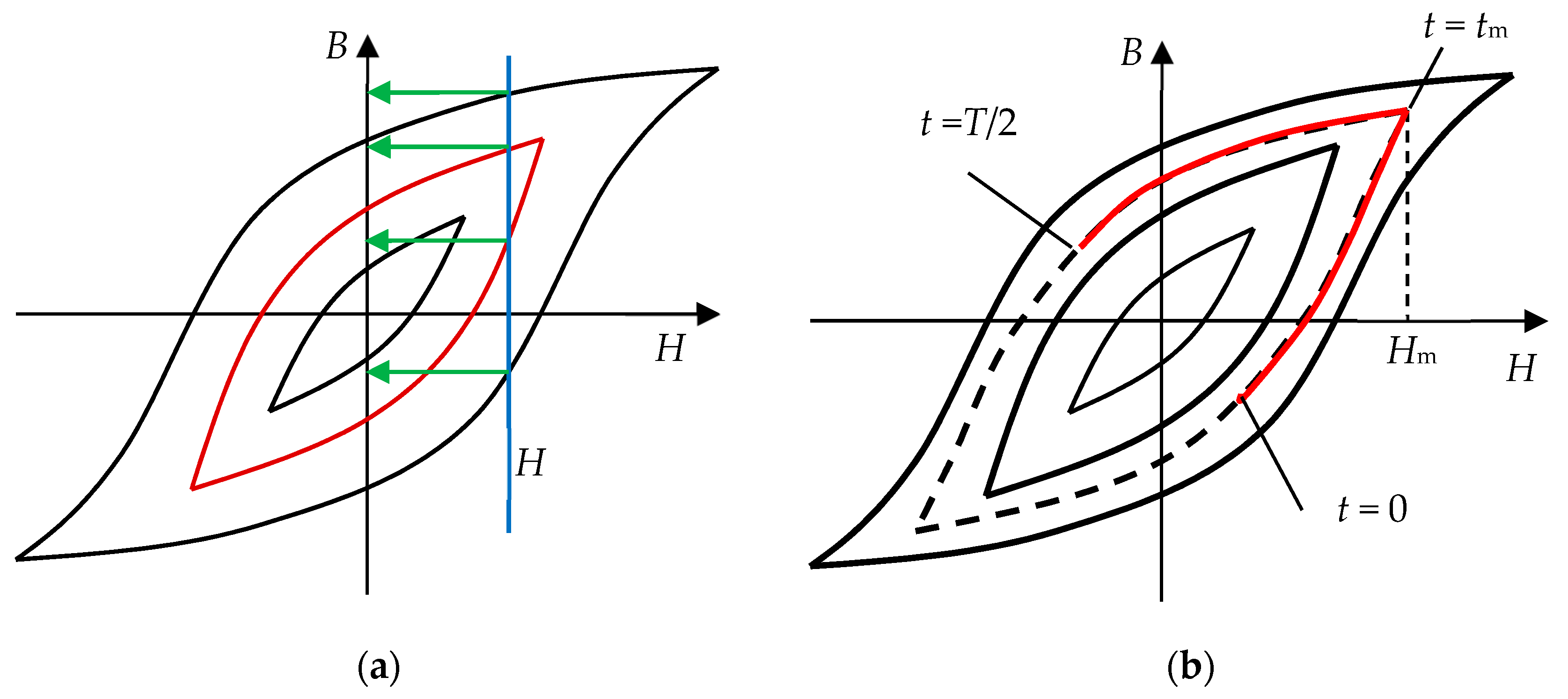
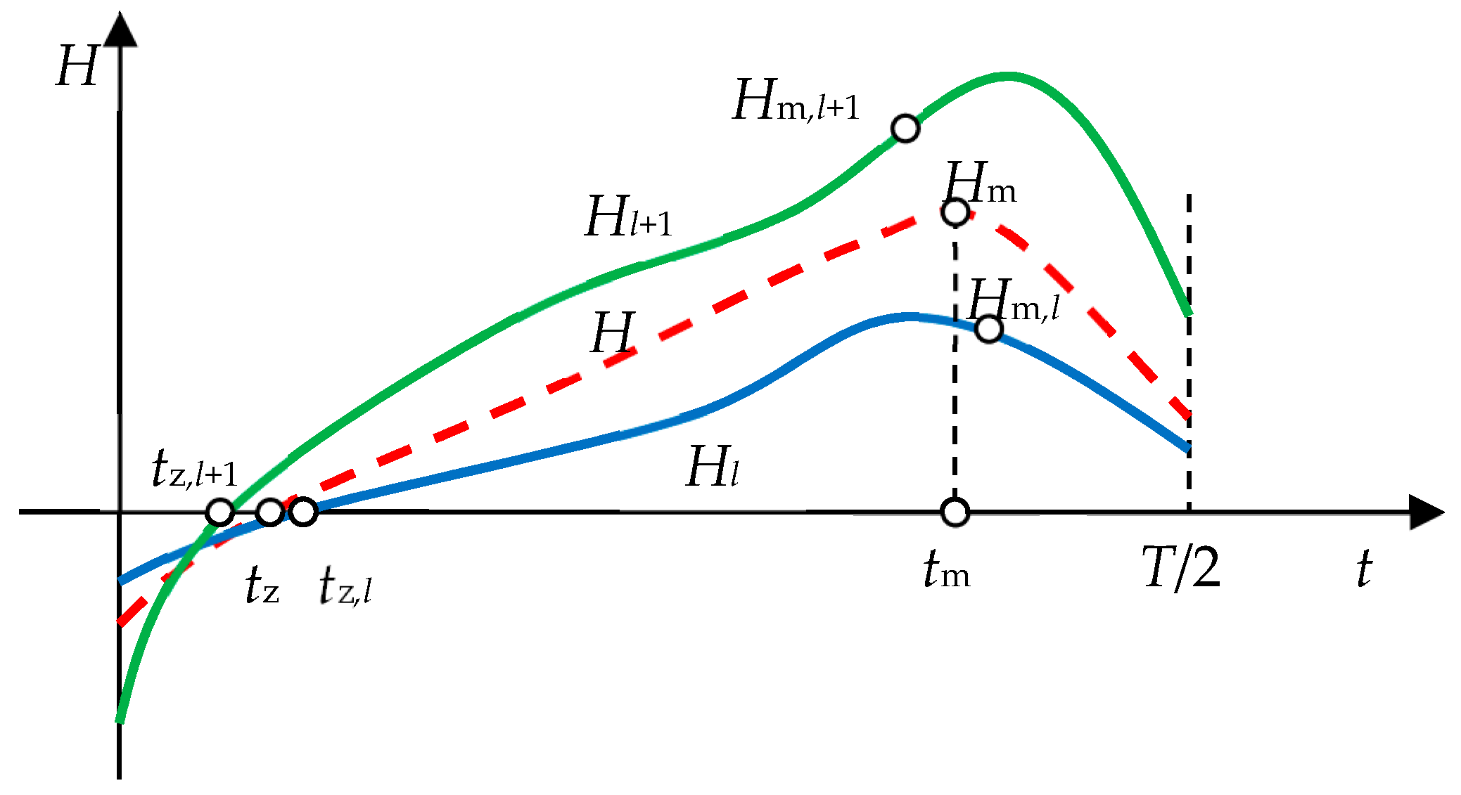
2.2. Conversion between H and B Fields

Conversions between H and B fields, denoted briefly as f_HB(B) or f_BH(H), are crucial steps in the algorithm (see Equations (8) and (11)). When using the magnetization curves without hysteresis taken into account, the conversion is simple and unique. But for the family of measured magnetic hysteresis loops, there are several problems associated with the conversion. Two of them are depicted in Figure 3a: which hysteresis loop should be selected, and which branch of the chosen hysteresis loop should be taken? It is not possible to convert uniquely between single values of H and B field, but it is possible for waveforms. Let H(t) be a known half waveform of H field obtained from Equation (7), and the corresponding B(t) is required. Suppose that H(t) initially increases up to H_m, which is reached for time t_m, and then H(t) decreases. First of all, the maximum value of H(t) is searched for—this allows the appropriate loop to be selected (assuming there is one loop with given H_m). The selection usually requires interpolation between two neighboring loops (see Figure 3b). Then, time t_m such that H(t_m) = H_m is determined. Finally, the loop is broken into the lower and upper branch, and the lower branch is used for t < t_m whereas the upper one for t > t_m. It is tempting to assume that $H\left(0\right)=-H_{\mathrm{m}}$ or $H\left(0\right)=0$, for example, to make the conversion easier. However, this cannot be warranted, because Equation (7) contains $H_{z0}^{\left(k\right)}\left(t\right)$, which can disturb this.

This procedure seems reasonable, but it is very sensitive to the loop slope—if dB/dH is large, then small changes in H result in large changes in B; this leads to problems with convergence of the algorithm for solving Maxwell’s equations. Moreover, the conversion fails when loops deviate from the “regular” shapes with one local maximum, because sometimes the lower branch has segments with negative slope. Therefore, a different method for conversion between H and B fields is proposed here. Measurement results in a list of H field waveforms, {H_l(t)}, and the corresponding list of B field waveforms, {B_l(t)}, where l numbers the measured loops. When plotted in (H, B) coordinates, the corresponding hysteresis loops family is obtained. The above-described method of H ↔ B conversion consists in a direct use of loops, whereas the proposed one uses the waveforms rather than loops. For further convenience, the lists are sorted so that the maximum values of H and B field increase. Moreover, the waveforms are adjusted so that B_l(0) = −B_max and B_l(T/2) = B_max. The idea of the algorithm is as follows:

• Given: H(t), {H_l(t)}, {B_l(t)};
• Construct linear interpolation between H_l(t) and H_l+1(t) in the following form:

  $$h\left(t\right)=\left(1-\theta \right)H_l\left(t+a\theta +b\right)+\theta H_{l+1}\left(t+a\theta +b\right),$$

  (13)

  and detect l, θ, a and b to satisfy h(t) = H(t) at some characteristic times or cases (the origin of Equation (13) is explained below);
• Use detected values of l, θ, a, b to calculate:

  $$B\left(t\right)=\left(1-\theta \right)B_l\left(t+a\theta +b\right)+\theta B_{l+1}\left(t+a\theta +b\right).$$

  (14)

The inverse conversion B(t) to H(t) is analogous.

The value of l determines waveforms B_l(t) and B_l+1(t) between which the interpolation takes place, $\theta$ is the interpolation factor, and aθ + b is required to take into consideration a possible time displacement. The assumed interpolating functions given by Equations (13) and (14) can be justified in the following manner. In the simplest form, the linear interpolation between waveforms $H_l$ and $H_{l+1}$ is as follows: $h\left(t\right)=\left(1-\theta \right)H_l\left(t\right)+\theta H_{l+1}\left(t\right)$. However, this form does not allow for possible time displacement of the waveforms. To permit time displacement the interpolating function should have the following form: $h\left(t\right)=\left(1-\theta \right)H_l\left(t+\mathsf{\Delta }{t}_l\right)+\theta H_{l+1}\left(t+\mathsf{\Delta }{t}_{l+1}\right)$, where $\mathsf{\Delta }{t}_l$ and $\mathsf{\Delta }{t}_{l+1}$ are certain constants. A bit more general form uses linear interpolation also between $\mathsf{\Delta }{t}_l$ and $\mathsf{\Delta }{t}_{l+1}$ as follows: $\mathsf{\Delta }t=\left(1-\theta \right)\mathsf{\Delta }{t}_l+\theta \mathsf{\Delta }{t}_{l+1}$, which can be written as $\mathsf{\Delta }t=a\theta +b$. As a result, Equation (13) represents the linear interpolation both in arguments (time) and values ($H$ field). A similar interpolation given by Equation (14) is used for $B$ field.

The values of $l$, $\theta$, $a$ and $b$ can be found in various ways, which usually lead to slightly different values, because equation h(t) = H(t) seldom can be satisfied for all times. Therefore, additional assumptions are required. First of all, it is expected that if H(t) can be found in {H_l(t)}, possibly after some time displacement, then h(t) should reflect this. This leads to the following equations:

$$\theta =0:H\left(t\right)=H_l\left(t+b\right),\theta =1:H\left(t\right)=H_{l+1}\left(t+a+b\right).$$

(15)

To establish a and b, some specific time must be assumed. One choice could be the time when H(t) reaches its maximum, but certain waveforms H_l(t) have more than one local maximum. Therefore, a better choice seems the time when H(t) is zero, because the time seems unique over one half period. Of course, there are two possibilities—time t_z when H(t) increases, and time t_z + T/2 when H(t) decreases after the half period. Let us take the first one. It will be called the ascending zero of H(t), i.e., H(t_z) = 0 and dH/dt > 0 for t = t_z. Hence, b = t_z,l − t_z and a = t_z,l+1 − t_z,l, where t_z,l and t_z,l+1 are ascending zeros of H_l and H_l+1, respectively. Then Equation (13) becomes:

$$h\left(t\right)=\left(1-\theta \right)H_l\left(t+\Delta t\right)+\theta H_{l+1}\left(t+\Delta t\right),$$

(16)

where:

$$\Delta t=a\theta +b=\left(1-\theta \right)t_{z,l}+\theta t_{z,l+1}-t_z.$$

(17)

Now it is necessary to find l and θ. To do this, equity h(t) = H(t) for certain t is required. Again, there are various possibilities to select the time. Based on the numerical experiments, we decided to use t = t_m, where t_m is such that H(t_m) = maxH(t) ≡ H_m. Then, solving equation H_m = h(t_m) yields:

$$\theta =\frac{H_{\mathrm{m}}-H_l\left(t_{\mathrm{m}}+\Delta t\right)}{H_{l+1}\left(t_{\mathrm{m}}+\Delta t\right)-H_l\left(t_{\mathrm{m}}+\Delta t\right)}.$$

(18)

This is a nonlinear equation with respect to θ, because Δt is a function of θ. If necessary, it can be solved numerically, but for close t_z,l+1 and t_z,l, which is a typical situation, it is convenient to use its approximate form as follows:

$$\theta =\frac{H_{\mathrm{m}}-H_{\mathrm{m},l}}{H_{\mathrm{m},l+1}-H_{\mathrm{m},l}},$$

(19)

where:

$$H_{\mathrm{m},l}=H_l\left(t_{\mathrm{m}}+t_{\mathrm{z},l}-t_{\mathrm{z}}\right).$$

(20)

Subsequent values of l in Equation (19) yield various solutions for θ. To stay within interpolation, θ should be in interval [0, 1], which allows l to be selected. If this is not possible, extrapolation is used with the last two waveforms and θ > 1. The final procedure in step 2 for determining l, θ, a and b is as follows:

2a.

Find the maximum value of H(t): H_m = maxH(t);

2b.

Find time t_m such that H(t_m) = H_m;

2c.

Find the ascending zero of H(t), i.e., time t_z < t_m such that H(t_z) = 0;

2d.

Construct a list of values H_m,l using Equation (20);

2e.

Find waveforms between which to interpolate, i.e., find such l that H_m,l ≤ H_m < H_m,l+1; if this is not possible, use the last two waveforms;

2f.

Calculate the interpolation factor using Equation (19);

2g.

Calculate a, b and the time displacement using Equation (17).

Such a procedure has the necessary property that when H(t) = H_l(t), then B(t) = B_l(t). The other desired property is that derivative dB/dH does not matter at all. There is no need to break the loops into branches, and the loops can have swings or infinite dB/dH values. The disadvantage is that when the shape of H(t) differs much from given set of waveforms {H_l(t)}, it is difficult to predict the behaviour of the algorithm, making the conversion problematic. However, the tests showed the procedure works quite well. The periodicity, symmetry and continuous nature of H_l(t) and H(t) mean the waveforms have exactly one ascending zero and reach a maximum value. Typically, the situation is as in Figure 4, in which two exemplary consecutive waveforms, H_l(t) and H_l+1(t), are shown, and also certain waveform H(t) is depicted together with some characteristic points.

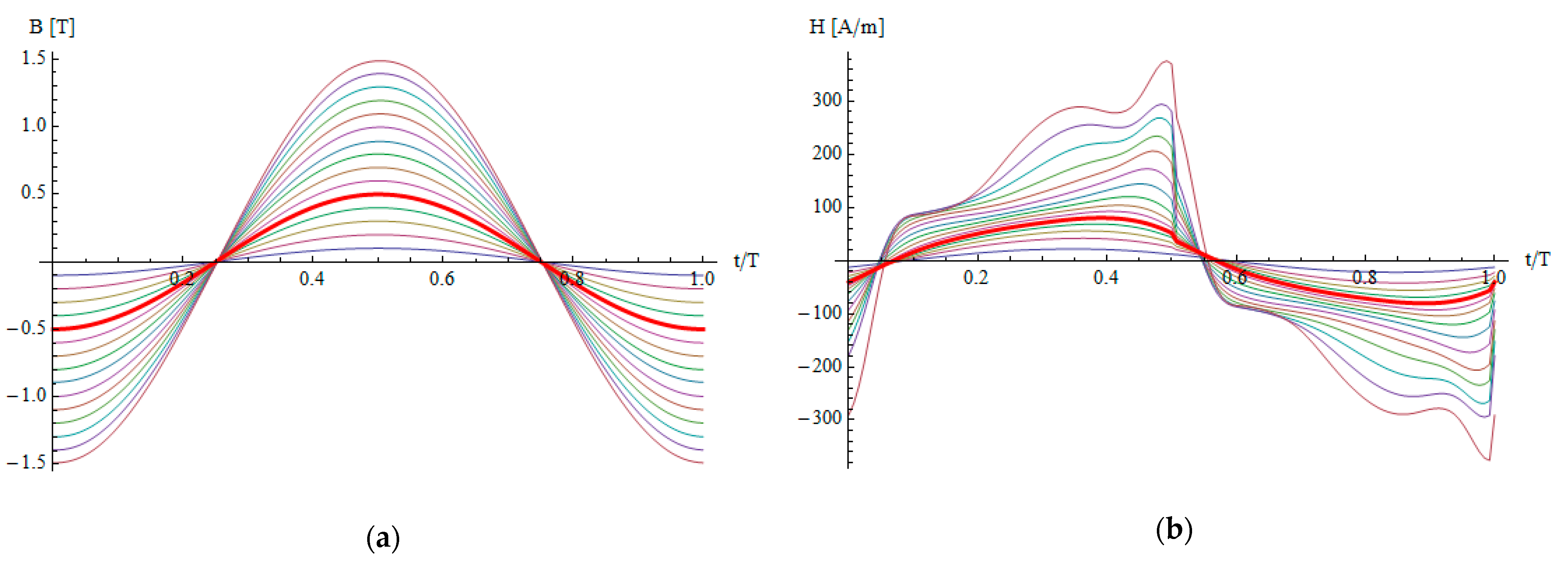
3. Results and Discussion

The algorithm was verified by calculating the macroscopic eddy current loss for three materials given in

Table 1. Specification of magnetic materials used in calculations.

Parameter	Material M1	Material M2	Material M3
Type	Non-oriented steel JNEX (6.5% Si-Fe)	Non-oriented steel M530-65A (3.2%Si-Fe)	Grain-oriented steel ET122-30 (3% Si-Fe)
Thickness (g)	0.1 mm	0.65 mm	0.3 mm
Conductivity (σ)	1.22 MS/m	2.56 MS/m	2.08 MS/m
Frequency (f)	10–400 Hz	5–400 Hz	10–1600 Hz
Magnetic flux density range (B)	0.1–1.2 T	0.1–1.6 T	0.1–1.5 T

. The materials have various thickness and include both non-oriented and grain-oriented steels.

The magnetic characteristics of materials M1 and M2 were measured on a MAG-RJJ-2.0 computer system, and for M3—on a REMACOMP C-200 measurement set [26]. The exemplary hysteresis loops for material M3 for f = 1000 Hz are shown in Figure 5a, whereas the corresponding waveforms {H_l(t)} and {B_l(t)} are depicted in Figure 6a,b. The lower branches of the some loops have swings with negative dB/dH, which disturb the conversion between H and B field via direct use of loops. The proposed method of conversion described in Section 2.2 allows us to use the waveforms and avoid the abovementioned problems.

In addition, plots in Figure 5b–d show the hysteresis loops of the three materials for B_m = 0.5 T and several frequencies. As the frequency grows, the loops become wider, which is related to the skin effect. In material M1, the growth is smallest due to small thickness of the sheet. In materials M2 and M3, the widening of loops is much more significant.

The values of parameters in the algorithm were as follows:

• Maximum relative error: ϵ = 0.001;
• Maximum number of iterations: k_max = 40;
• Number of time intervals per half the period: N_T = 32;
• Number of spatial segments per half the thickness: N_g = 20.

Figure 7a,b shows exemplary waveforms of the B and H fields obtained for material M2, B_m = 1 T and a frequency of 50 Hz. Figure 8a,b illustrates the convergence in the iterative process.

The algorithm was convergent for almost all cases, and the number of iterations required for convergence usually was below 10. In case of a lack of convergence, the calculations were repeated with smoothing used to reduce the numerical noise, so that all harmonics of order 4 or higher with an amplitude no greater than 10% of the highest amplitude in the spectrum were treated as noise and removed, as described in [25].

The results of calculations are presented in Figure 9, Figure 10, Figure 11, Figure 12 and Figure 13, in which the percentage relative deviation defined as follows:

$${\delta }_{\mathrm{P}}=\frac{P_{cl}^{alg}-P_{cl}}{P_{cl}}\times 100\%,$$

(21)

is presented for the three materials, where $P_{cl}^{alg}$ is the loss calculated via the algorithm given by Equation (5), and P_cl is the classical loss as follows:

$$P_{cl}=\frac{\pi \gamma f{B}_{\mathrm{m}}^2}{2\mu }\frac{\sinh \gamma -\sin \gamma }{\cosh \gamma -\cos \gamma },\gamma =g\sqrt{\pi \sigma \mu f}.$$

(22)

The relationship (22) describes the classical loss in macroscopic terms, neglecting the domain wall structure. There are loss models taking into account the domain structure, e.g., the Pry–Bean model [27], but these are not considered in the analyzed case. Instead, the magnetic permeability μ in the above formula was calculated as B_m/H_max, and not assumed to be a constant value as in the classical approach.

The nonlinearity itself does not affect significantly the value of the classical loss. For the considered materials, the percentage deviation δ_P does not exceed 3% (the largest value is for material M2, frequency 200 Hz and magnetic flux density 0.4 T). On the other hand, the magnetic hysteresis considerably changes the eddy current loss. The deviation reaches up to several dozen percent. The largest deviations are observed for magnetic flux density in the range 0.2–1.0 T. For the tested materials, the largest deviation occurred in the following cases:

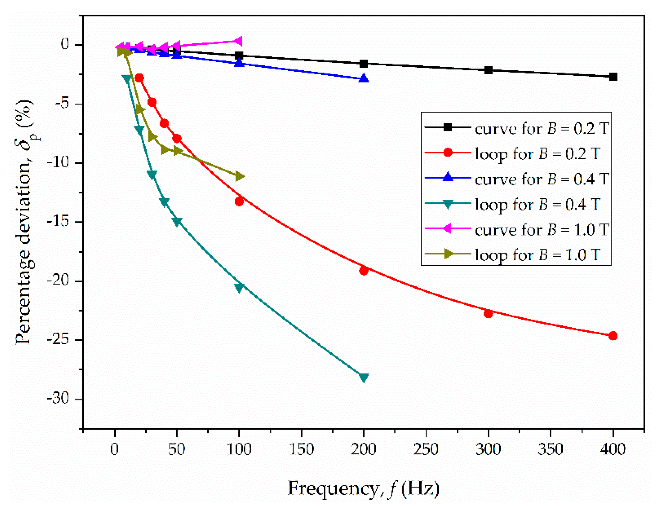
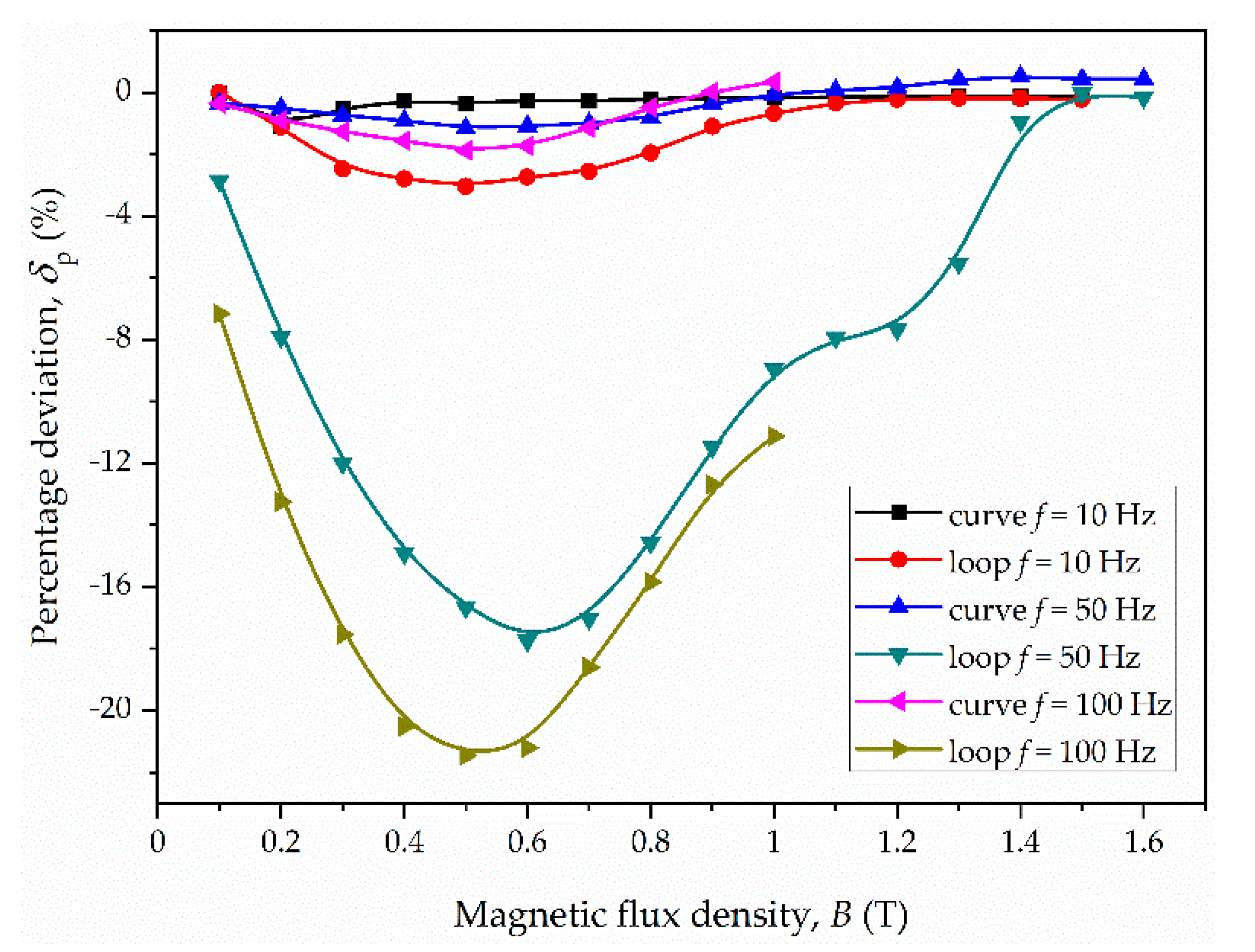
• M1: −2.6% for f = 20 Hz and B_m = 0.6 T;
• M2: −28% for f = 200 Hz and B_m = 0.4 T;
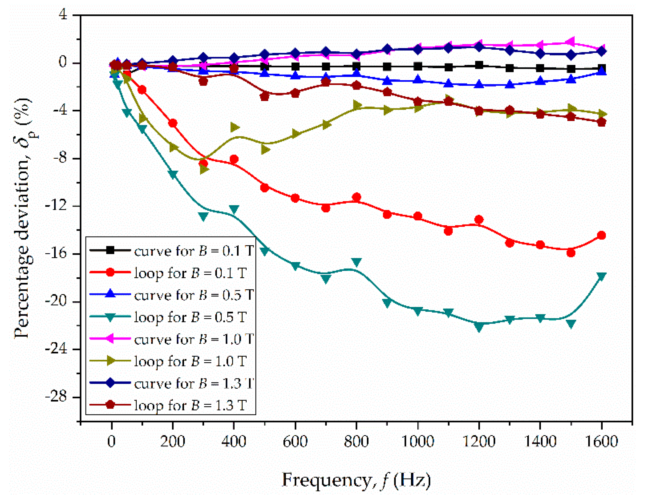
• M3: −24% for f = 1500 Hz and B_m = 0.4 T.

In general, the deviations are the larger the higher the frequency and the thicker the sample, i.e., the stronger the skin effect (due to non-uniform distribution of magnetic flux).

Usually, the deviation given by Equation (21) is negative when magnetic hysteresis is taken into account. It follows that neglecting the magnetic hysteresis overestimates the eddy current loss. This may lead, for example, to misidentification of the excess loss in Bertotti’s approach. The fact that including the hysteresis loops into calculations shows smaller eddy currents loss agrees with the theoretical considerations, which models the hysteresis via complex permeability [28].

It is also interesting that the deviation is largest for middle values of magnetic flux density (see Figure 9, Figure 10 and Figure 11), and not for the values near to saturation, for example. This is because the middle loops affect the current distributions much more than those for strong saturation in comparison to the case of neglecting the hysteresis.

4. Conclusions

In the paper, an algorithm of including the magnetic hysteresis phenomenon into calculating the macroscopic eddy currents loss was proposed. It is based on direct using the hysteresis loops obtained from measurement without any specific model of magnetization, which can be regarded as an advantage from the practical point of view. Moreover, a new idea of conversion between B and H fields based on waveforms was also proposed to improve the algorithm performance. It was shown that it works well for wide class of hysteresis loops. The calculations carried out for various types of electrical steels showed that neglecting the hysteresis overestimates the classical loss. On average, the effect is the stronger the higher frequency and the thicker the sheet. The largest differences occur for intermediate values of magnetic flux density.

In future research the proposed approach to calculating the eddy current loss will be examined for different types of soft magnetic materials, such as amorphous or nanocrystalline alloys. Moreover new improvements of the algorithm will be considered. Another direction of future research is developing the algorithm for B-H characteristics taken under other types of excitations, e.g., sinusoidal H field.

References

1. Barranger, J. Hysteresis and Eddy-Current Losses of Transformer Lamination Viewed as an Application of the Pointing Theorem; NASA Technical Note; National Aeronautics and Space Administration: Washington, DC, USA, 1965; p. D-3114. [Google Scholar]
2. Bertotti, G. Hysteresis in Magnetism; Academic Press: San Diego, CA, USA, 1998. [Google Scholar]
3. Pieper, W.; Gerster, J. Total power loss density in a soft magnetic 49% Co-49% Fe-2% V-alloy. J. Appl. Phys. 2011, 109, 07A312. [Google Scholar] [CrossRef]
4. Bertotti, G. A general statistical approach to the problem of eddy current losses. J. Magn. Magn. Mater. 1984, 41, 253–260. [Google Scholar] [CrossRef]
5. Bertotti, G. General properties of power losses in soft ferromagnetic materials. IEEE Trans. Magn. 1988, 24, 621–630. [Google Scholar] [CrossRef]
6. Bertotti, G. Some considerations on the physical interpretation of eddy current losses in ferromagnetic materials. J. Magn. Magn. Mater. 1986, 54, 1556–1560. [Google Scholar] [CrossRef]
7. Zirka, S.E.; Moroz, Y.I.; Marketos, P.; Moses, A.J. Loss separation in nonoriented electrical steels. IEEE Trans. Magn. 2010, 46, 286–289. [Google Scholar] [CrossRef]
8. Kollár, P.; Birčákováa, Z.; Füzera, J.; Bureš, R.; Fáberováb, M. Power loss separation in Fe-based composite materials. J. Magn. Magn. Mater. 2013, 327, 146–150. [Google Scholar] [CrossRef]
9. Kollár, P.; Olekšáková, D.; Vojtek, V.; Füzer, J.; Fáberová, M.; Bureš, R. Steinmetz law for ac magnetized iron-phenolformaldehyde resin soft magnetic composites. J. Magn. Magn. Mater. 2017, 424, 245–250. [Google Scholar] [CrossRef]
10. Sun, H.; Li, Y.; Lin, Z.; Zhang, C.; Yue, S. Core loss separation model under square voltage considering DC bias excitation. AIP Adv. 2020, 10, 015229. [Google Scholar] [CrossRef] [Green Version]
11. Li, H.; Wang, L.; Li, J.; Zhang, J. An improved loss-separation method for transformer core loss calculation and its experimental verification. IEEE Access 2020, 8, 204847–204854. [Google Scholar] [CrossRef]
12. Zhao, Z.; Hu, X. Modified loss separation in FeSi laminations under arbitrary distorted flux. AIP Adv. 2020, 10, 085222. [Google Scholar] [CrossRef]
13. Olekšáková, D.; Kollár, P.; Jakubčin, M.; Füzer, J.; Tkáč, M.; Slovenský, P.; Bureš, R.; Fáberová, M. Energy loss separation in NiFeMo compacts with smoothed powders according to Landgraf’s and Bertotti’s theories. J. Mater. Sci. 2021, 56, 12835–12844. [Google Scholar] [CrossRef]
14. Chwastek, K.; Szczygłowski, J.; Wilczyński, W. Modeling magnetic properties of high silicon steel. J. Magn. Magn. Mater. 2010, 322, 799–803. [Google Scholar] [CrossRef]
15. Pluta, W. Some properties of factors of specific total loss components in electrical steel. IEEE Trans. Magn. 2010, 46, 322–325. [Google Scholar] [CrossRef]
16. De Campos, F.M. Loss Separation Model: A Tool for Improvement of Soft Magnetic Materials. Mater. Sci. Forum 2016, 869, 569–601. [Google Scholar] [CrossRef]
17. De Campos, F.M. Interpretation of loss separation with the Haller-Kramer model. Acta Phys. Pol. A 2019, 136, 705–708. [Google Scholar] [CrossRef]
18. Bereźnicki, M. The influence of skin effect on the accuracy of eddy current energy loss calculation in the electrical sheets. In Proceedings of the 2015 Selected Problems of Electrical Engineering and Electronics (WZEE), Kielce, Poland, 17–19 September 2015; IEEE: New York, NY, USA, 2016. [Google Scholar] [CrossRef]
19. Butler, O.I.; Sarma, M.R. Relaxation methods applied to the problem of a.c. magnetization of ferromagnetic laminae. Proc. IEE Part II Electr. Eng. 1951, 98, 389–397. [Google Scholar] [CrossRef]
20. Zakrzewski, K.; Pietras, F. Method of calculating the electromagnetic field and power losses in ferromagnetic materials, taking into account magnetic hysteresis. Proc. Inst. Electr. Eng. 1971, 118, 1679–1685. [Google Scholar] [CrossRef]
21. Petrun, M.; Steentjes, S.; Hameyer, K.; Ritonja, J.; Dolinar, D. Effects of saturation and hysteresis on magnetisation dynamics. COMPEL Int. J. Comput. Math. Electr. Electron. Eng. 2015, 34, 710–723. [Google Scholar] [CrossRef]
22. Takahashi, N.; Sakura, T.; Cheng, Z. Nonlinear analysis of eddy current and hysteresis losses of 3-D stray field loss model (Problem 21). IEEE Trans. Magn. 2001, 37, 3672–3675. [Google Scholar] [CrossRef]
23. Górecki, J.; Nowak, L.; Poltz, J. Numerical calculation of eddy current losses in conductive ferromagnetic plate. Electr. Hear. 1976, 22, 677–685. [Google Scholar]
24. Bereźnicki, M.; Jabłoński, P. Calculating macroscopic eddy current losses in ferromagnetic materials considering hysteresis loop. Pozn. Univ. Technol. Acad. J. Electr. Eng. 2018, 93, 205–214. [Google Scholar] [CrossRef]
25. Bereźnicki, M.; Jabłoński, P.; Najgebauer, M. Using measured hysteresis loop family in calculating the eddy current losses. In Proceedings of the 2018 Progress in Applied Electrical Engineering (PAEE), Koscielisko, Poland, 18–22 June 2018; IEEE: New York, NY, USA, 2018. [Google Scholar] [CrossRef]
26. Operating Instruction, REMACOMP® C-200; Magnet-Physik, Dr. Steingroever GmbH: Köln, Germany, 2017.
27. Pry, R.H.; Bean, C.P. Calculation of the energy loss in magnetic sheet materials using a domain model. J. Appl. Phys. 1958, 29, 532–533. [Google Scholar] [CrossRef]
28. Zakrzewski, K. The influence of magnetic hysteresis on the separation and distribution of power losses in ferromagnetic sheets. Rozpr. Elektrotechniczne 1971, 17, 431–446. (In Polish) [Google Scholar]
Figure 1. The geometry of the analyzed sample.
Energies 15 02869 g001
Figure 2. Block diagram of the algorithm.
Energies 15 02869 g002
Figure 3. Conversion HB: (a) problems of non-uniqueness—which loop to select for given H, and which B to select for given H and loop? (b) the loop corresponding to given H(t) (dashed line) is found via interpolation between two loops from measurements (thick solid lines).
Energies 15 02869 g003
Figure 4. Typical waveforms H(t), Hl(t) and Hl+1(t).
Energies 15 02869 g004
Figure 5. Exemplary hysteresis loops of the considered materials: (a) for material M3 and a frequency of 1000 Hz; (b) for material M1 and Bm = 0.5 T; (c) for material M2 and Bm = 0.5 T; (d) for material M3 and Bm = 0.5 T.
Energies 15 02869 g005
Figure 6. Waveforms of the B and H fields for material M3 and a frequency of 1000 Hz: (a) waveforms Bl(t); (b) corresponding waveforms Hl(t).
Energies 15 02869 g006
Figure 7. Half waveforms of the B and H fields at various depths in the M2 sample for Bm = 1 T and f = 50 Hz: (a) magnetic flux density; (b) the magnetic field intensity; the thick blue and thick magenta traces correspond to the surface and the middle of the sample, respectively; the three thin traces are for intermediate y coordinates; the dashed trace is for the value averaged throughout the sample.
Energies 15 02869 g007
Figure 8. Values of power loss (a) and error indicator (b) in subsequent iterations corresponding to Figure 7: (a) values of eddy current power loss expressed in W/kg; (b) values of δB = ΔBmax/Bm; in this case four iterations were enough to establish the results within assumed accuracy.
Energies 15 02869 g008
Figure 9. Percentage deviation for eddy current loss vs. magnetic flux density for material M1.
Energies 15 02869 g009
Figure 10. Percentage deviation for eddy current loss vs. magnetic flux density for material M2.
Energies 15 02869 g010
Figure 11. Percentage deviation for eddy current loss vs. magnetic flux density for material M3.
Energies 15 02869 g011
Figure 12. Percentage deviation for eddy current loss vs. frequency for material M2.
Energies 15 02869 g012
Figure 13. Percentage deviation for eddy current loss vs. frequency for material M3.
Energies 15 02869 g013