Article

Parameter Evaluation in Motion Estimation for Forecasting Multiple Photovoltaic Power Generation

1
Graduate School of Science and Technology, Tokyo University of Science, Noda 278-8510, Japan
2
Faculty of Science and Technology, Sophia University, Tokyo 102-8554, Japan
3
Faculty of Engineering, Information and Systems, University of Tsukuba, Tsukuba 305-8573, Japan
*
Author to whom correspondence should be addressed.
Energies 2022, 15(8), 2855; https://doi.org/10.3390/en15082855
Submission received: 27 January 2022 / Revised: 25 March 2022 / Accepted: 6 April 2022 / Published: 13 April 2022
(This article belongs to the Topic Solar Thermal Energy and Photovoltaic Systems)

Abstract

:
The power-generation capacity of grid-connected photovoltaic (PV) power systems is increasing. As output power forecasting is required by electricity market participants and utility operators for the stable operation of power systems, several methods have been proposed using physical and statistical approaches for various time ranges. A short-term (30 min ahead) forecasting method had been proposed previously for multiple PV systems using motion estimation. This method forecasts the short time ahead PV power generation by estimating the motion between two geographical images of the distributed PV power systems. In this method, the parameter λ , which relates the smoothness of the resulting motion vector field and affects the accuracy of the forecasting, is important. This study focuses on the parameter λ and evaluates the effect of changing this parameter on forecasting accuracy. In the periods with drastic power output changes, the forecasting was conducted on 101 PV systems. The results indicate that the absolute mean error of the proposed method with the best parameter is 10.3%, whereas that of the persistence forecasting method is 23.7%. Therefore, the proposed method is effective in forecasting periods when PV output changes drastically within a short time interval.

1. Introduction

Reducing greenhouse gas emissions caused by power production can effectively address climate changes [1]. Therefore, the installation of photovoltaic (PV) power generation systems is significantly increasing with the decreasing installation costs [2], reaching 39 GW in 2010 and 760 GW in 2020 [3]. However, as opposed to the existing dispatched power generations, the power generation of PV relies on the weather conditions, thus varying drastically and uncertainly. The high penetration of PV power generation makes it difficult to maintain the balance between demand and supply in electric power systems. This uncertain variability in PV generation can significantly impact the stable and economical operation of power systems [4,5]. Therefore, power system operators require forecasting of PV generation output; particularly, short-term forecasting is required to determine the need for demand response, and a quick-start generator is required for the stable operation of the power grid [4]. To date, different forecasting methods have been proposed for various time scales using solar radiation forecasting or direct PV power forecasting. PV forecasting can be classified into persistent forecasting, physical approach, and statistical approach [6,7]. The physical approach forecasts solar irradiance data from a numeric weather predictor atmospheric model. A common approach for regional PV output using numeric weather predictor (NWP) data is to upscale a set of representative regional PV systems. Saint-Drenan et al. [8] proposed a method to probabilistically forecast the PV output of the entire forecast area from the reference PV power and meteorological data obtained from NWP. Ma et al. [9] proposed a method to correct the NWP irradiance using the measured irradiance and optimized the prediction model using the particle swarm optimization algorithm. Statistical approaches include forecasting models based on a learning process that uses variables with historical influence. These forecasting models attempt to reduce errors by using the difference between the model’s forecasted and actual data. Therefore, this approach has high-forecasting accuracy for time periods during which the model input patterns are smooth. However, forecast errors increase during periods associated with abrupt changes in weather variables commonly referred to as “drastic change periods”, such as solar radiation, temperature, and humidity [6]. Statistical methods can be divided into two categories, namely time-series-based and artificial intelligence forecasting models [6]. Artificial intelligence is a popular technique for forecasting PV output generation. Among them, NN is one of the most used forecasting models. Bacher et al. [10] reported that autoregression model forecasting can be effective for short-term forecasting based on the results obtained using NWP, observed PV data, and data from both sources. Reikard [11] estimated the solar radiation intensity using the autoregressive integrated moving average (ARIMA) method and compared it with that obtained from the artificial neural network (ANN) method. Neural networks use different sets of input data to forecast future output patterns and improve the accuracy of the model by carefully selecting different influential parameters. Pedro and Coimbra [12] implemented an ANN method optimized by a genetic algorithm (GAs/ANN) and compared it with the persistent forecast, ARIMA method, and k-nearest neighbors (kNN) method. They verified that GAs/ANN is superior to the other forecast methods. Zhou et al. [13] used two long short-term memory models to forecast the temperature and PV output and combined them to enhance the forecast accuracy. Behera et al. [14] implemented an optimal design methodology for an extreme learning machine-based forecasting model of a PV system and compared its results with those of existing models, such as the backpropagation model. Alamoudi et al. [15] analyzed the performance of photovoltaic panels using an adaptive neural network-based fuzzy inference system (ANFIS) to determine the self-consumption and sufficiency rates of a PV system, and used response surface methodology (RSM) to determine the optimal operating conditions of the PV panels. They used the ANFIS to analyze the performance of photovoltaic panels to determine the self-consumption and sufficiency rates of PV systems, and a response surface methodology (RSM) to determine the optimal operating conditions of the PV panels. In addition to these approaches, forecasting methods based on image processing techniques have been proposed. Studies have been conducted to estimate solar radiation from satellites and grand-based sensors. Hammer et al. [16] proposed a method for estimating solar radiation from satellite images and a statistical method for estimating the movement of clouds. Perez et al. [17] reported that satellite-derived cloud motion-based forecasts are better models for short-term forecasts than NWP-based solar radiation forecasts. Bright et al. [18] proposed a method for selecting reference PVs to support PV output nowcasts from satellite images. Feng et al. [19] developed a deep convolutional neural network for global horizontal irradiance one hour ahead of the sky image. Chu et al. [20] proposed a reforecasting model to improve the forecasting by reforecasting with an ANN and optimizing with a GA from the sky racking technique, ARIMA, and kNN forecasting. Chow et al. [21] estimated cloud motion from the optical flow method using a sky-imaging system, and the best forecasting may be obtained depending on the smoothness parameter.
Table 1 presents a brief description and summary of these forecasts. The effective timescales in Table 1 are summarized in [22].
The aforementioned short-term forecasting method tends to yield a high error during periods when PV output changes abruptly. In contrast to these studies, our previous proposal focused on the temporal transition of output power from geographically distributed PV systems [23]. Therefore, this approach aims to reduce forecasting errors during periods of abrupt changes in weather conditions for multiple PV systems at different locations. The output power distribution of irregularly located PV systems was converted into a regularly arranged mesh distribution with the same latitude and longitude intervals. Forecasting was conducted by estimating the motion of mesh distribution. In the future, the smart grid will be upgraded to capture the PV output power; therefore, this method is economical for short-term forecasting, as it allows for predictions without additional equipment.
The existing method uses the optical flow for forecasting, wherein the motion field between two consecutive images is estimated. This motion field is obtained by minimizing the objective function, comprising the data term and regularization term, by using the variational method [24,25]. The parameter λ of the regularization term is a model of the smoothness of the motion field obtained using this function. This parameter is important because the obtained motion field is highly affected by the parameter. Previously [23,26], the mesh size and interpolation method for blank values when converting to a mesh distribution were determined. In [23], the proposed method was evaluated based on the forecasting results by only λ = 1.0 . In addition, the mesh size determined in the previous studies was small relative to the geographic transitions of actual weather conditions, and the estimations based on this mesh size can drive the objective function to local minimum. Therefore, there were many periods in which the estimated motion vectors did not match the actual motions in rapidly changing weather conditions. In this study, a multiscale approach was used to address this issue. This makes it possible to obtain a motion vector field that is more appropriate to the actual motions by finding the global minimum of the objective function, and to properly evaluate the effect of changing the parameter λ . The purpose of this study is to examine the effect of changing this parameter λ and to show the improvement of the prediction results from previous studies. In this study, the prediction of 101 PV power systems is executed with several values of the parameter λ , and the prediction error distribution of each PV is evaluated. The PV distribution in Japan (latitude 31.20 ° 6′–39 ° 80′ and longitude 129 ° 60′–141 ° 60′) was normalized every 30 min for one year from 2013 to 2014, converted to geographically distributed mesh data, the motion of the NV distributions was estimated, and then the forecast was evaluated. The PV output volatility is important when evaluating a forecast. Certain periods exist, such as clear days, when it is easy to forecast the PV generation. These times reduce the error difference when evaluating the motion estimations of each parameter, making it difficult to evaluate the parameters. Pedro and Coimbra [12] reported that developing seasonal models for each period of variability should improve the evaluation of the forecasting method. The objective of this method is to forecast the PV output during periods when the output of multiple PVs changes. As the changes in the PV output over a wide range differ from place to place, capturing the changes in multiple PV outputs is difficult. Therefore, in this study, the period when the output of PVs in a certain area within a 15-km-radius in Japan changed drastically within 30 min was extracted and evaluated. This paper evaluates the proposed method with the multiple PV output changed periods in a certain area where the output changes are correlated to each other. The contributions of this study can be summarized as follows.
  • A method is proposed for evaluating multiple PV generation forecasts when the PV output changes drastically.
  • The parameter that makes the best forecast for motion estimation reduces the error by 56.6% compared to that of the persistence forecasting. It is an effective forecasting method for periods when PV output changes drastically.
  • The characteristics of forecasting a wide range of PV outputs using a motion estimation method are presented.
The remainder of this paper is organized as follows. Section 2 describes the data preprocessing, estimation, and evaluation methods of the proposed method. Section 3 explains the characteristics of the motion estimation, forecasting results at drastic change periods, and reasons for the errors. Finally, Section 4 concludes the study.

2. Materials and Methods

This section describes the input data, forecasting methods, and evaluation methods. Figure 1 depicts the flowchart of the proposed method. The forecast method uses the power generation output of the PV and position data as input and performs the forecast using an image processing approach. In this method, prior to motion estimation, the geographically distributed power output of PVs is preprocessed to enable image processing. The power output of each PV system is forecasted based on the estimation results. Additionally, this method changes the smoothness parameter of the motion estimation and evaluates it during periods when the output changes drastically. In this section, first the conditions under which the period was extracted and then the evaluation methods are described.

2.1. Dataset

The dataset used in this study is the actual data of the output power from 5097 PV systems measured at 30 min intervals from 1 August 2013, to 31 July 2014, in Japan. Therefore, the forecast timescale Δ t was set to 30 min. Table 2 presents an outline of the dataset.

2.2. Preprocessing

The proposed method uses motion estimation, which is an image processing method. To apply the motion estimation to forecast the output of geographically distributed PV systems with various power ratings and forms, the output power data were normalized and converted to mesh data. The following process was implemented to achieve this.

2.2.1. Normalization

The output power from the PV systems is affected by the panel size, material, azimuth angle, tilt angle, and installation location. Therefore, normalization is necessary to compare numerous geographically distributed PV systems. In this study, NV of the output power is defined as indicated in Equation (1).
NV t = P t P 2 w t
where P t denotes the actual PV power output at a specific time t , and P 2 w t represents the highest power output at the same time t in the previous two weeks. Figure 2 depicts the concept of normalization implemented on 14 July 2014. Figure 2a shows the output power P t of a PV system on 14 July 2014 (orange line) and that observed on the previous 14 days from 30 June to 13 July 2014 (gray lines); their maximum values P 2 w t at the corresponding times are also indicated (red line). The two-week period is selected under the assumption that at least one sunny day exists, and the seasonal change in sun elevation is negligible during this period. Figure 2b depicts NV t at different times on 14 July 2014 calculated using Equation (1).

2.2.2. Conversion to Mesh Data

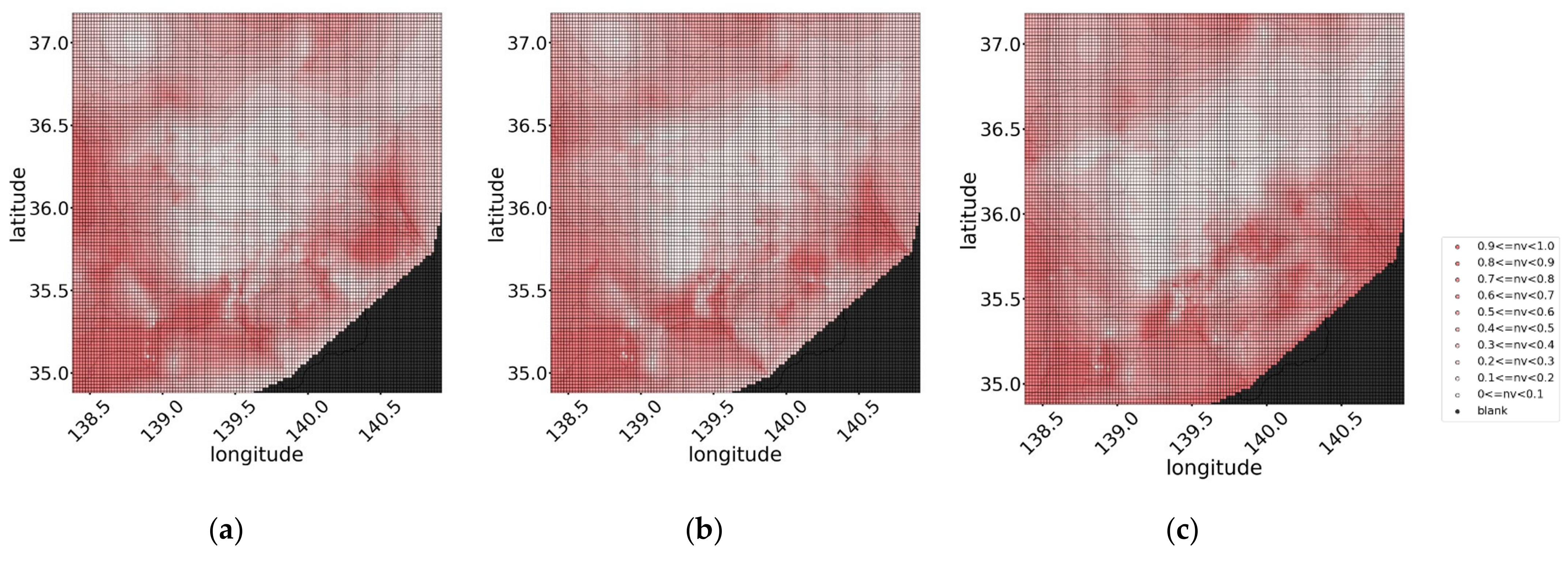
In the proposed method, the irregular geographical distribution of NV values is converted to a mesh distribution, which is the distribution data aligned at equal intervals in the east–west and north–south directions to adapt it to image processing methods. The NV value of each parcel in the regularly arranged distribution with equally spaced widths of latitude and longitude were obtained from the average of the NVs of PV systems located in the parcel. In this study, the width of the mesh was set to 0.02 in latitude and longitude, based on the reports of a previous study [22]. Figure 3 depicts the conversion diagram to mesh data; Figure 3a shows the actual locations of the PV systems and their NVs at 11:00 on 14 July 2014, are classified by color, and Figure 3b shows the mesh distribution at that time. In Figure 3b, the parcels with no corresponding PV are considered blank values and are indicated in black. If several blank values exist in the mesh data, the motion estimation cannot be performed. Therefore, we performed interpolation (Figure 3c) based on Delaunay triangulation using “grid data”, which is a function of MATLAB 2020a [27].

2.3. Motion Estimation

The geographical distribution of NV is assumed to move over time based on the movement of elements affecting weather conditions, such as clouds. The optical flow method, which involves image processing, was used to analyze the motion [25,26]. Assuming that NV is invariant and moves linearly in the time interval Δ t , the NVs expressed as f x , y , t during the period from time t Δ t to t can be expressed as indicated in Equation (2).
f x u x , y , t Δ t ,   y v x , y , t Δ t , t Δ t = f x , y , t
where x , y denotes the position of NV in the east–west and north–south directions, and u x , y , t and v x , y , t represent the velocities of NV at position x , y and at time t in the east–west and north–south directions, respectively. A regulation term is defined considering that adjacent motion vectors tend to be aligned. The NV data term E D and regularization term E s can be determined using Equations (3) and (4), respectively, in each mesh.
E D 2 x , y , t = f x u x , y , t Δ t ,   y v x ,   y , t Δ t ,   t Δ t f x , y , t 2
E S = u x , y , t 2 + v x , y , t 2
where = x ,   y T represents the partial differential operator. The energy function is expressed as shown in Equation (5) while introducing a weight coefficient λ , which determines the extent to which u and v are spatially aligned. The value of λ is adjusted to minimize the estimation error.
J x , y , t = E D 2 x , y , t + λ E s x , y , t d x d y
The vector distribution can be obtained by solving the energy function minimization problem, and the solution is expressed in Equations (6) and (7), which are Euler–Lagrange equations.
λ T u E D x f = 0
λ T u E D x f = 0
The detailed solution and algorithm are reported in [24].
As mentioned previously, the width of the mesh is 0.02 , which corresponds to 1.806 km and 2.219 km in the east–west and north–south directions, respectively, at latitude   35 ° 78   and   longitude   140 ° 04 . However, the motion vectors for 30 min may be longer than the mesh width. Sawada and Takahashi [28] analyzed the migration of precipitation areas and reported that the speed was distributed in the range of 2–8 m/s. Bosch and Kleissl [29] proposed a method to estimate the cloud velocity using three reference PV cells and inverter output in a 48 MW PV plant. From their analysis, they reported that the velocity of clouds is distributed in the range of 3–35 m/s based on the analysis.
A multiscale approach was used to avoid the local minima of the energy function indicated in Equation (5). This approach generates a rougher distribution with multiple size scales, seeks the global minimum, and propagates the solution gradually to finer scales. In this study, the Gaussian filter was used to generate a four-fold rougher distribution.
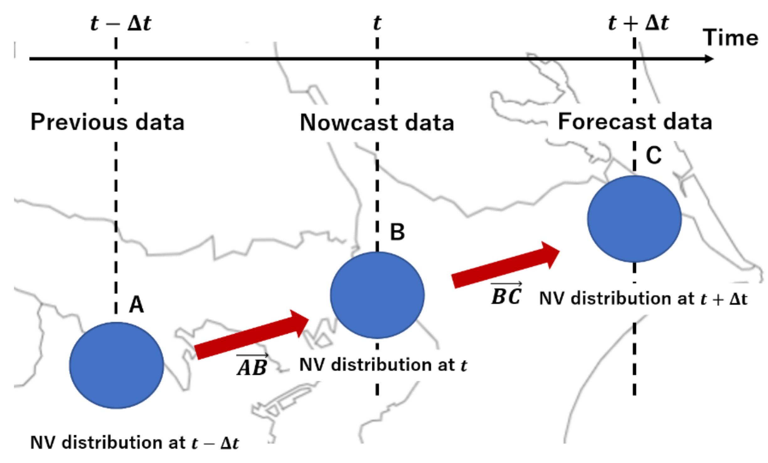
Figure 4 illustrates the motion estimation concept. Using the optical flow method, vector AB representing the NV of location A at time t Δ t and then moved to location B at time t is estimated. Assuming that the movement is a constant velocity linear motion and persists until t + Δ t , vector BC is obtained by moving vector AB in parallel. The forecasting distribution of all mesh at time t + Δ t is obtained by interpolating the location of C from each NV obtained from vector BC.

2.4. Error Evaluation Method

In this study, the periods when NV values of more than 80% of the PV systems changed to higher than 0.2 in 30 min are referred to as drastic change periods. Generally, PV power forecasting is difficult when a drastic change occurs. Periods with drastic changes were extracted to evaluate forecast errors under harsh conditions.
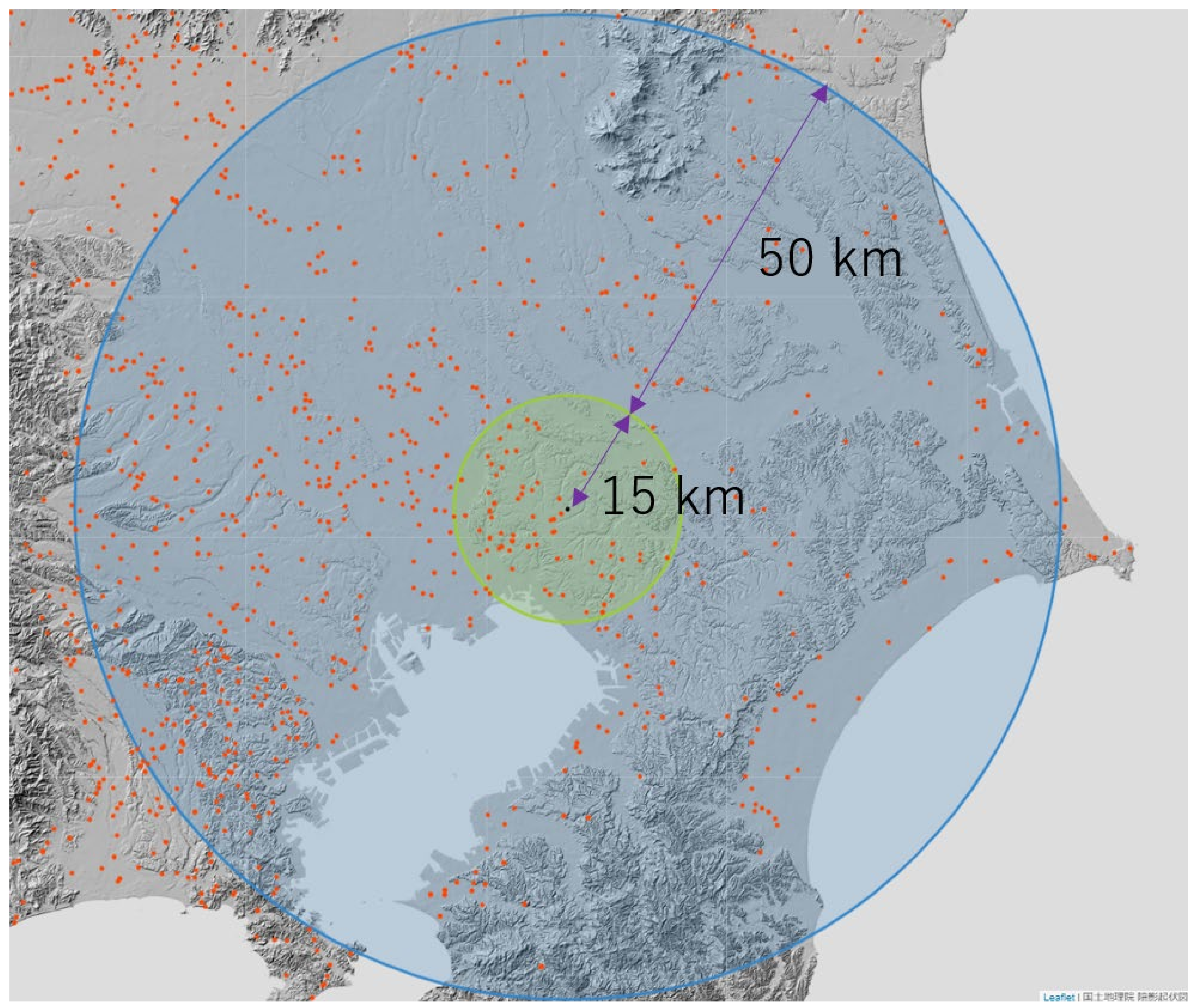
The forecast error is evaluated in a certain area, which is shown by the green circle in Figure 5, in the Kanto Region with 101 PV systems while varying λ , which is the parameter in the motion estimation, to minimize the error caused by the interpolation process. Table 3 summarizes the dataset of the evaluated area. The central point of the evaluated area is located at latitude   35 ° 78   and   longitude 140 ° 04 . Figure 4 depicts the area, wherein the green circle with a radius of 15 km denotes the evaluated area, and the blue circle with a radius of 65 km indicates the area that has probably been used to estimate NV distribution in the green area.
The absolute percent error (APE) is used as an evaluation method to examine the forecast error in periods during which the weather changes drastically, as indicated in Equation (8). Additionally, the definitions of the mean-absolute-percent error (MAPE) and root-mean-square error (RMSE) are indicated in Equations (9) and (10), respectively.
APE = P forecasted P observed P maximum × 100
MAPE = 1 N i = 1 N APE i
RMSE = 1 N i = 1 N ( P forecasted i P observed i ) 2
where N denotes the number of evaluated time steps, P forecasted represents the forecasted PV output, P obverved denotes the observed PV output, and P maximun indicates the maximum observed PV output for a year.

2.5. Comparison with Other Methods

In this study, persistence forecasting and ANN were implemented for comparison. As the influence of the sun elevation in a day is assumed to be represented by multiplying P 2 w t , the PV power output in persistence forecasting can be calculated using Equation (11).
P persistence t + Δ t = P 2 w t + Δ t × NV t
The ANN was used as a machine learning-based forecasting method and consists of an input layer, three hidden layers, and an output layer. The numbers of neurons in the three hidden layers are 768, 384, and 192. The rectified linear unit (ReLU) function was used as the activation function. Cross–validation was performed by dividing the continuous time into four parts to obtain the validation error. Input data are month, day, hour, solar radiation, and temperature obtained from the Japanese Meteorological Agency. Herein, solar radiation represents the accumulated solar radiation from one hour before the forecast time. A detailed description of the model is given in [30]. A comparison between the ANN and the proposed method is shown in Section 3.2.

3. Results and Discussion

This section presents the forecast results of the motion estimation that were evaluated using 101 PVs in the evaluation area. Initially, the importance of extracting and evaluating the period in which the outputs change drastically was confirmed by comparing the forecasting results of days exhibiting a drastic change in the period with those obtained on a clear day. Subsequently, the error distribution of the persistent forecasting and the nine parameters at the extracted times were evaluated to determine the best parameter. Finally, the forecast results for a certain period were analyzed to determine the cause of the forecast error at the period when the error was reduced by changing the parameters and at periods when the forecast error could not be reduced by any of the parameters. This analysis improves the understanding of the characteristics of the motion estimation method.

3.1. Characteristics of Motion Estimation Based on Weather

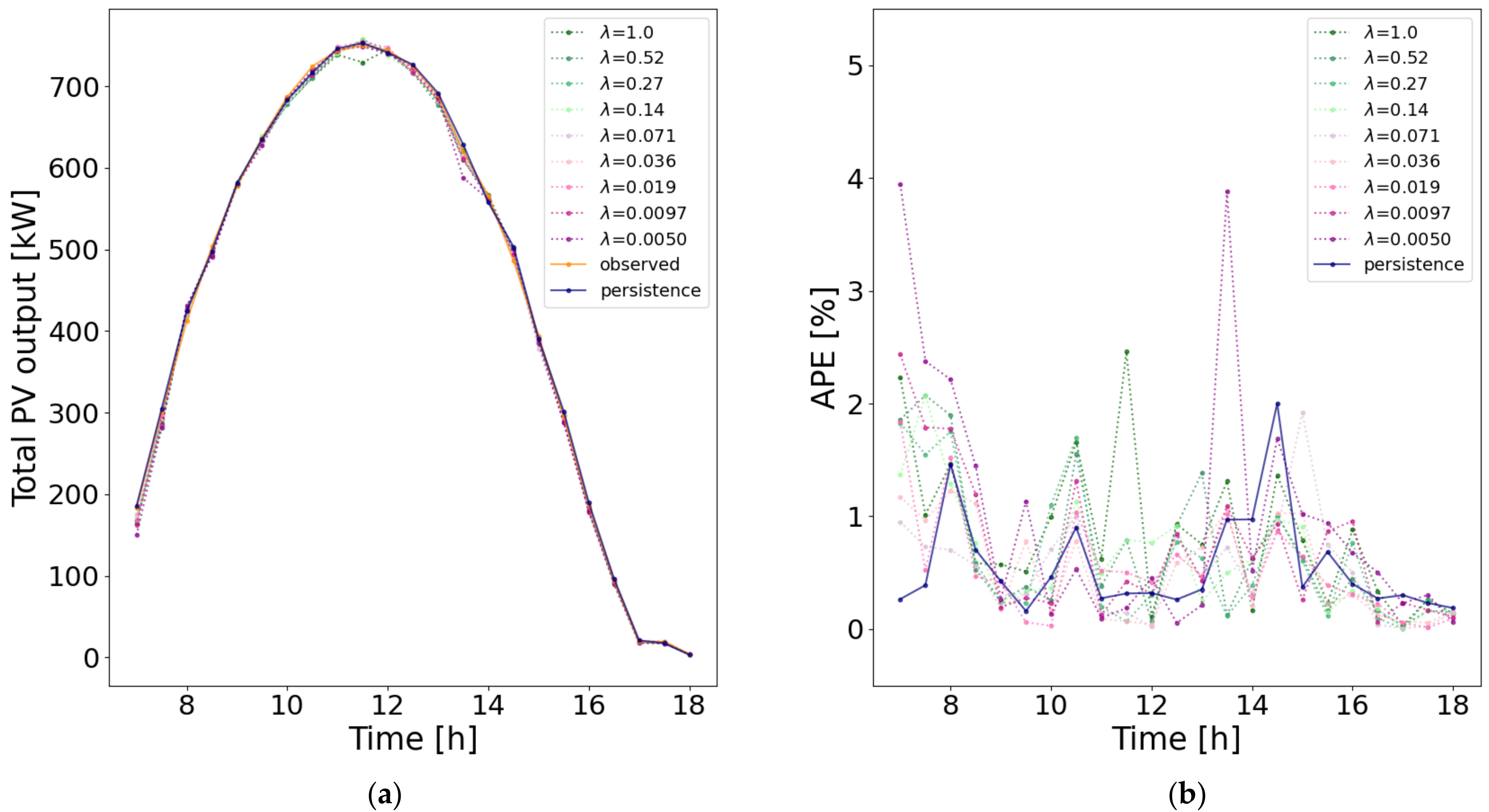
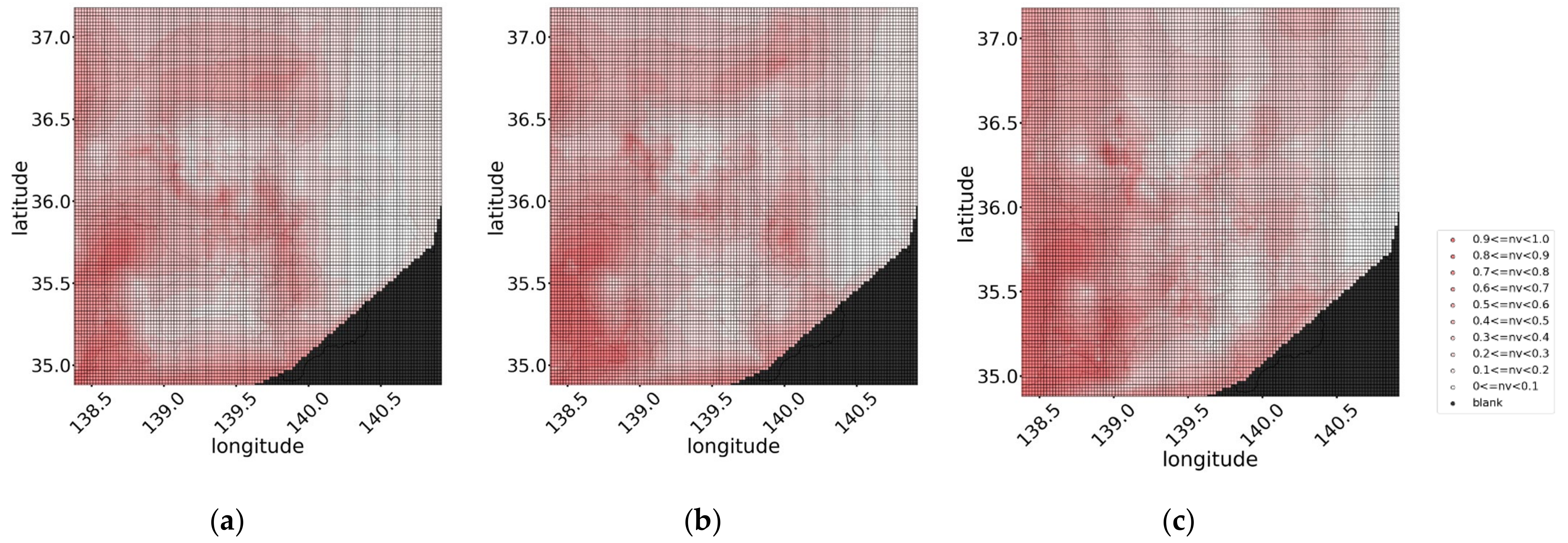
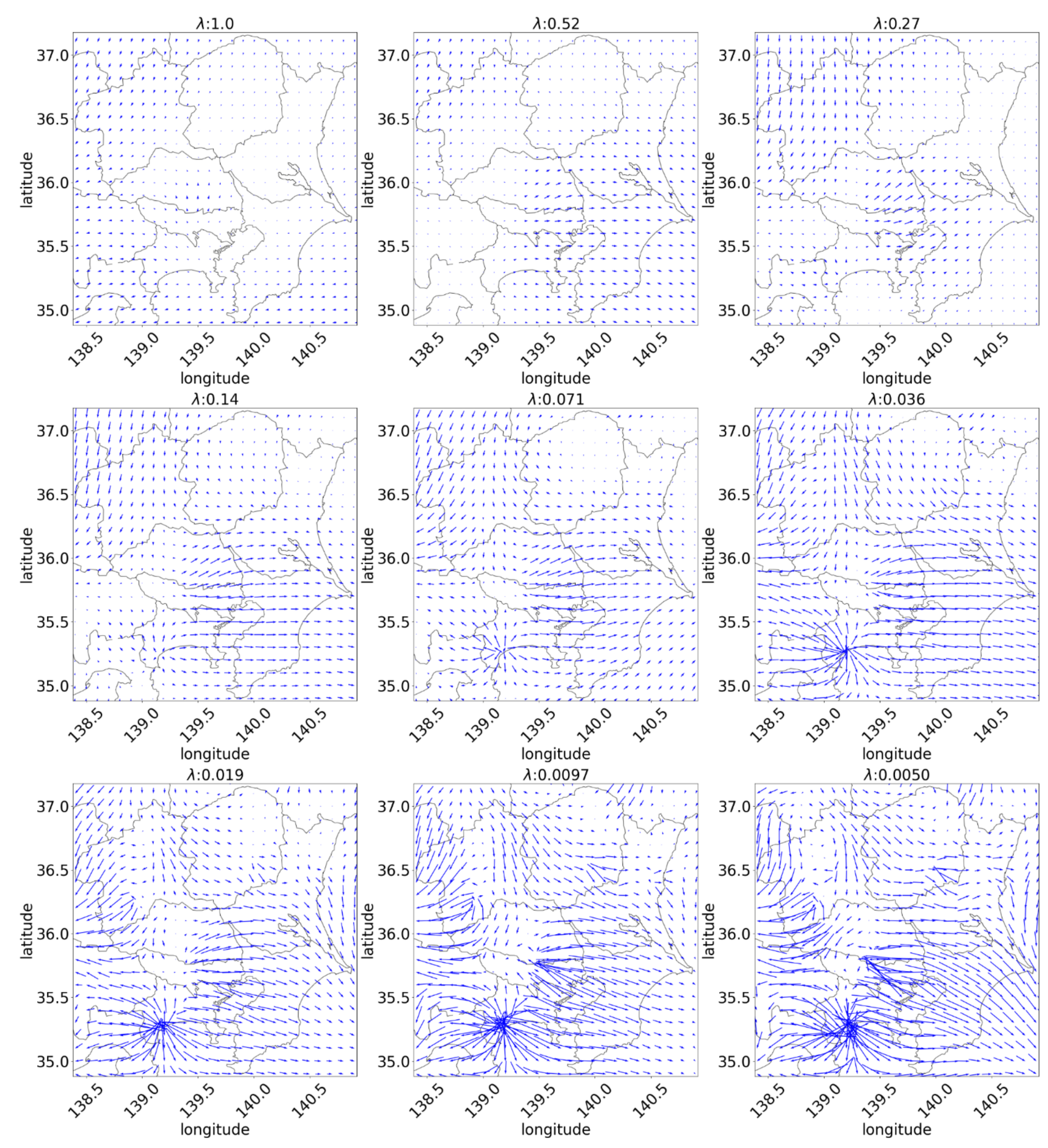
Figure 6a depicts the sum of the power generation of 101 PV systems. Figure 6b shows the error of the total output in the evaluation area. Table 4 summarizes the daily average MAPE and RMSE calculated on 16 March 2014. Figure 7 shows the time variation of the observed NV distribution at the period used to estimate NV motion and the forecasting period, respectively, at 12:00 on 26 March 2014. Figure 8 illustrates the distribution of motion vectors between 11:00 and 12:00 calculated to forecast the NV distribution at 12:00 on 16 March 2014, under clear weather conditions.
Figure 7 indicates that the change of NVs is small in the evaluation area; the forecast error of the proposed method is similar to that of the persistence forecasting. On a clear day, motion estimation estimates small movements, as depicted in Figure 8.
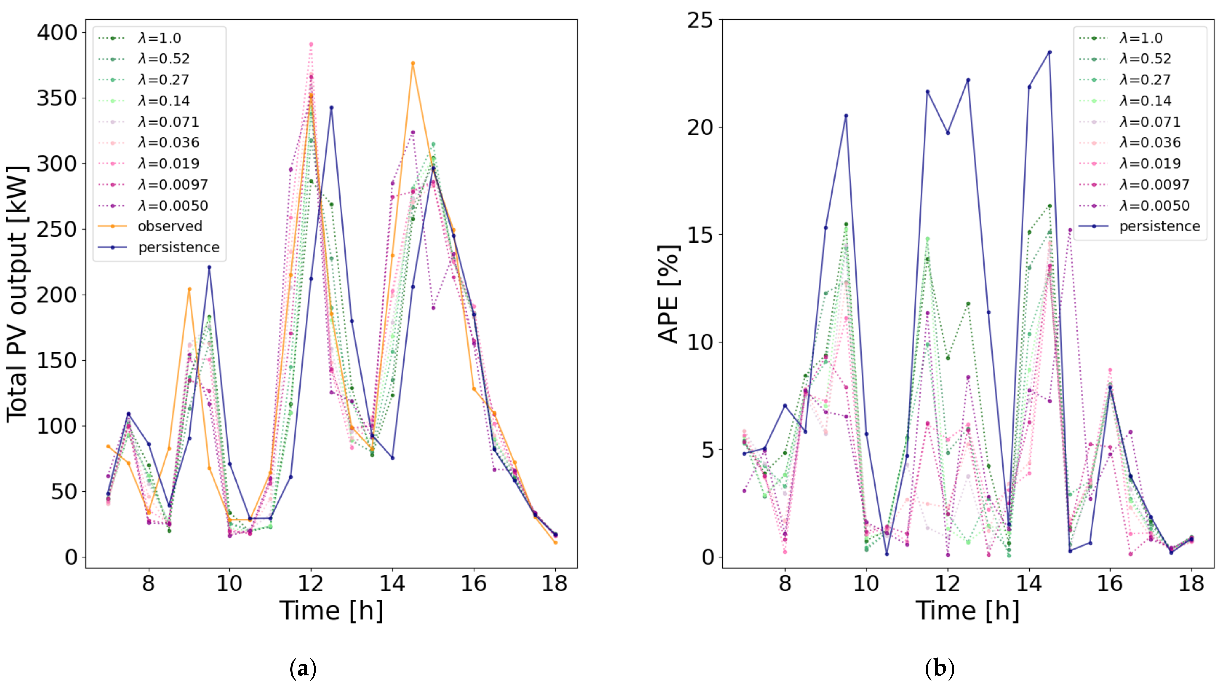
Figure 9a,b depict the sum of the power generation of 101 PV systems and the corresponding error of the total output in the evaluation area, respectively. Table 5 summarizes the daily average MAPE and RMSE of the total output calculated on 5 September 2013. Figure 10 shows the time variation of the observed NV distribution at the period used to estimate NV motion and the forecasting period, respectively, at 12:30 on 5 September 2013. Figure 11 depicts the distribution of motion vectors between 11:00 and 11:30 calculated to forecast the NV distribution at 12:30 on 5 September 2013, when the output power changed drastically.
Figure 10 indicates that there was a visible change in the distribution of NVs in the evaluation area; thus, a drastic change occurred in the output power, and the large motion vectors of the NV distribution were calculated, as depicted in Figure 11. In such a period, the forecast error of the proposed method is expected to reduce in comparison with that of the persistence forecasting. Figure 11 indicates that the estimation results differ according to the value of parameter λ .
This method is classified as a short-term forecast, and PV has a higher correlation with the previous output as the forecast time-horizon scale is shorter. Additionally, the result of motion estimation is close to that of the persistence forecast when the period NV distribution remains unchanged.
In this study, the proposed method is compared with persistence forecasting and ANN to verify its effectiveness, and parameter λ is evaluated for the drastic change periods.

3.2. Evaluation of the Estimation Error

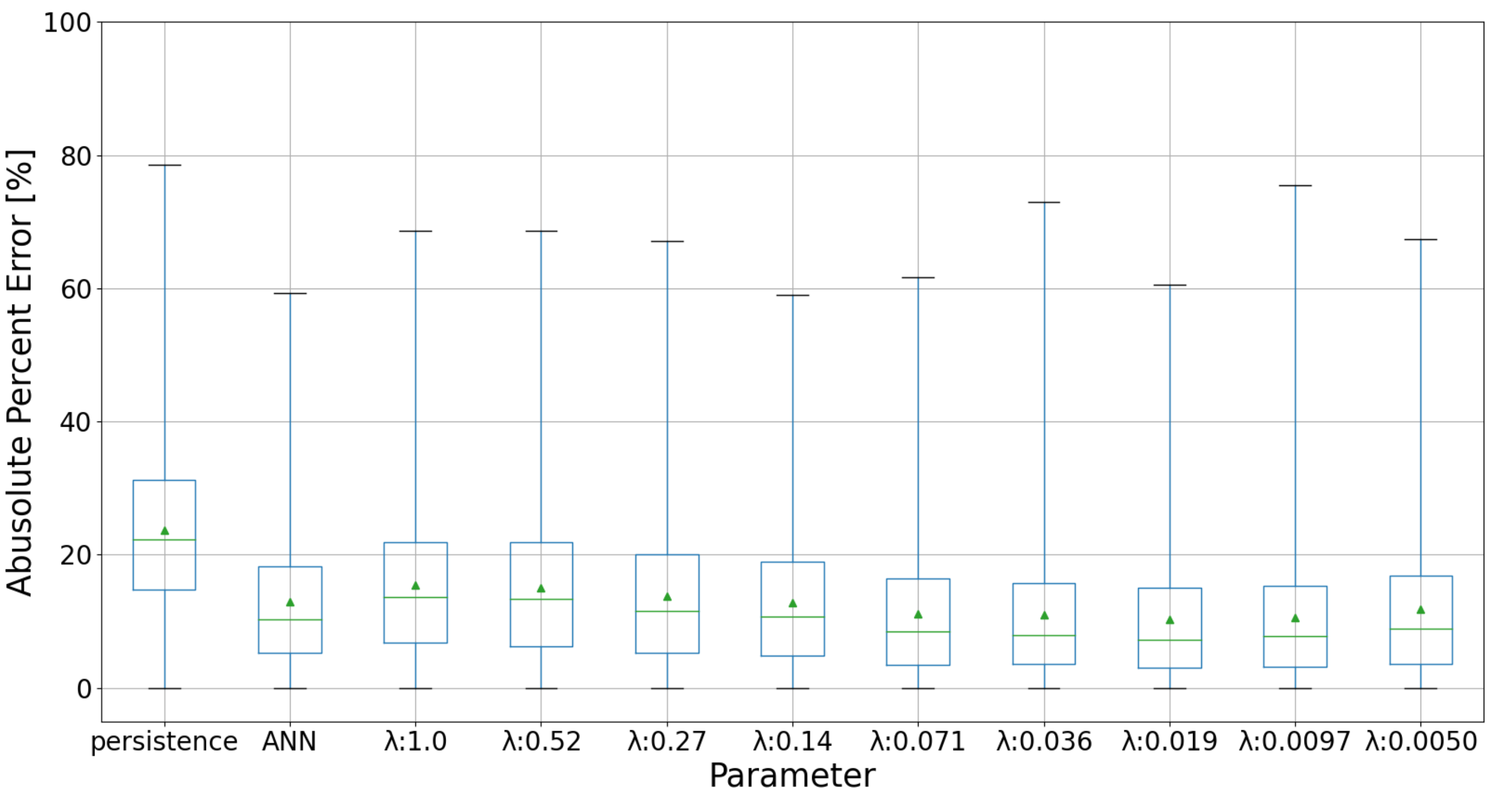
The estimation results of the proposed forecasting evaluated the motion estimation parameter λ and compared it with the persistence forecasting and ANN for periods when the output power varied drastically. Note that in this section, the ANN results are for the 96 units that could be forecasted in the ANN. Figure 12 depicts a box plot of the estimation errors for the periods in the evaluated area, Table 6 shows the mean, median, and standard deviation of the errors. In the case of persistence forecasting, the mean was 23.7%, and the median was 22.2%, and for the ANN, the mean was 13.0% and the median was 10.2% In the case of proposed forecasting with the best motion estimation parameter λ = 0.019 , the mean was 10.3%, and the median was 7.20%. In other words, the means of the proposed forecasting with the best parameter reduced in comparison with the persistence forecast (by 56.6%) and the ANN (by 20.8%).
The authors have applied the same forecasting method in other two regions in Japan: 122 PV systems in Kansai region and 26 PV systems in Chubu region. Furthermore, in these two regions, the forecasting errors by the proposed method with the best parameter λ ( λ = 0.019 in the case of Kansai region and λ = 0.036 in the case of Chubu region) were ~50% lower than those by the persistence forecast [31]. Therefore, it is confirmed that the proposed method is effective for forecasting periods with a drastic change in output power.

3.3. Results of Estimation Errors

The estimation errors observed in the proposed method can be attributed to two reasons, namely the pre-processing and motion estimation. During pre-processing, the influence of the differences in tilt angle and installation orientation of the PV arrays is not completely canceled out by the normalization process. Consequently, the representative value of each mesh used in the estimation is the average of all NV values of the corresponding PV systems in the mesh. Furthermore, certain errors are caused by the interpolation of NVs in areas with no data; errors on motion estimation occur when assumptions of NV invariance and NV having a constant velocity linear motion were inappropriate.
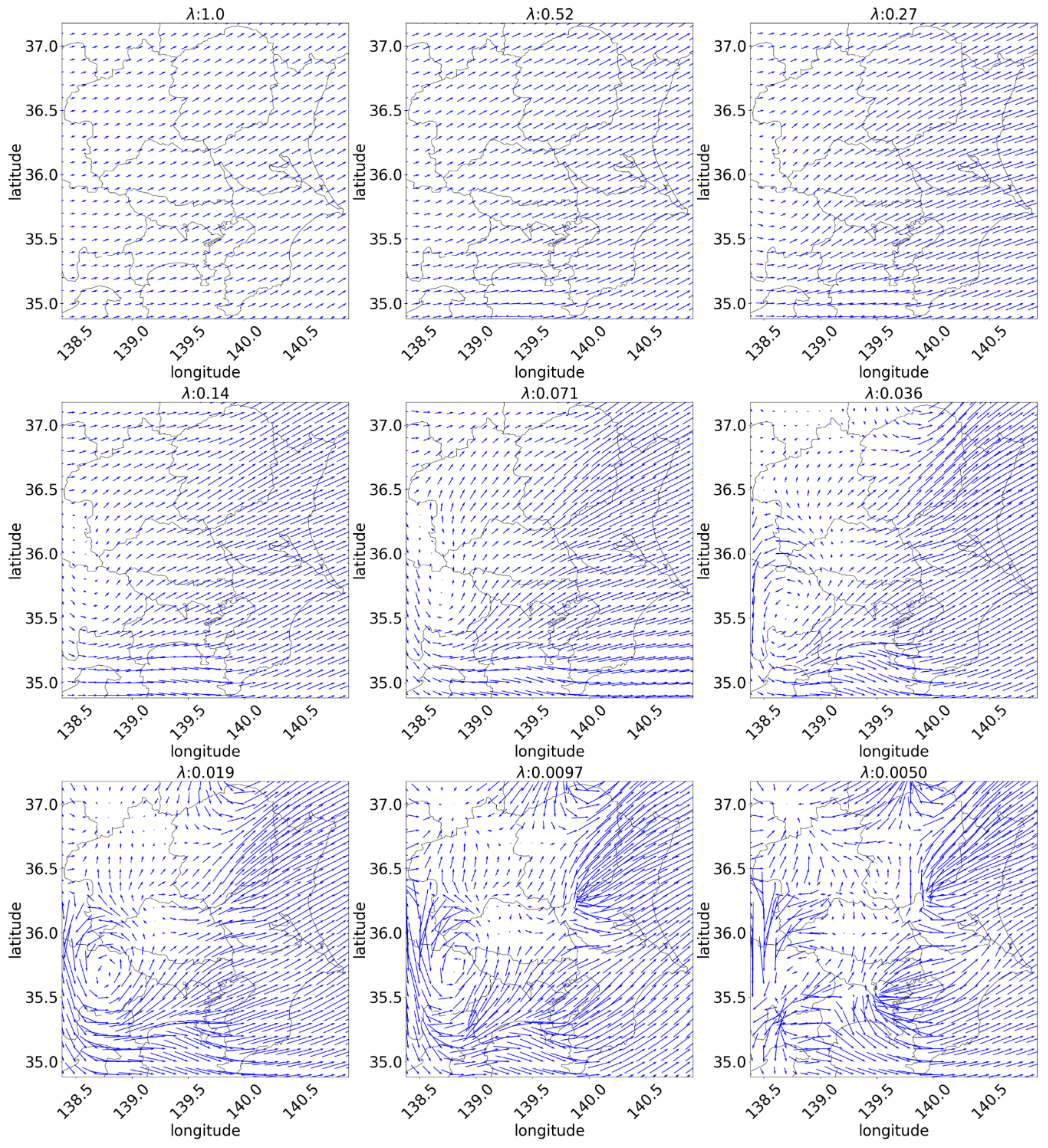
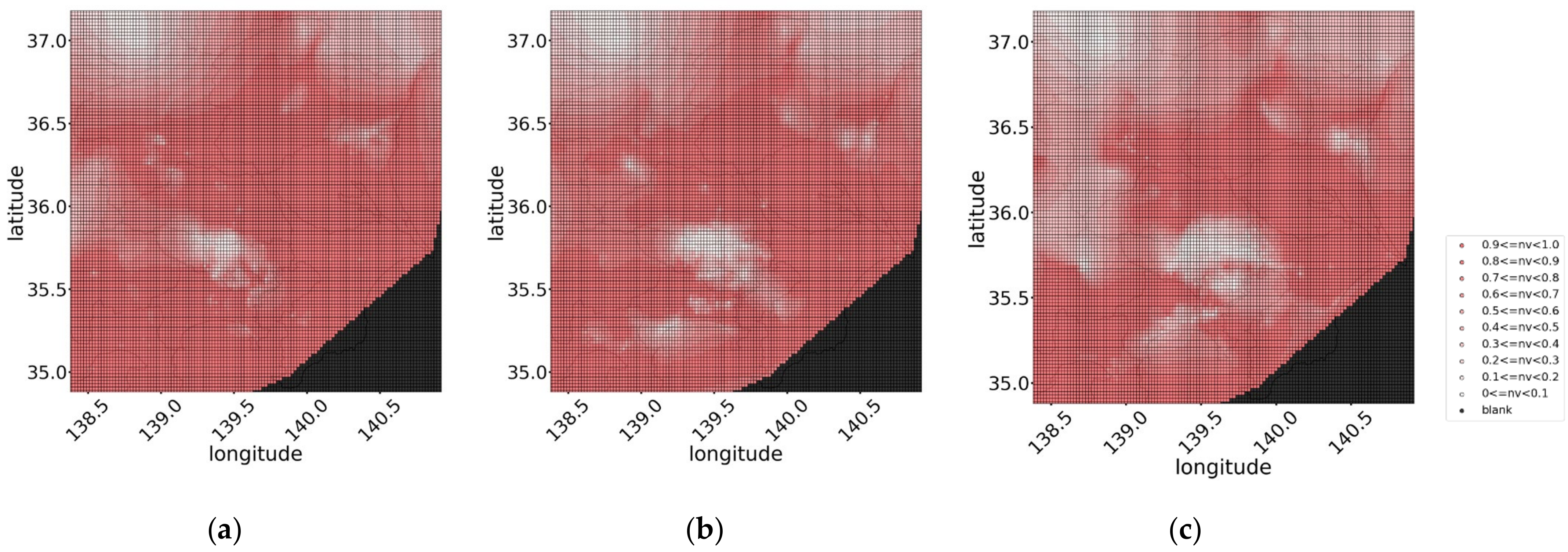
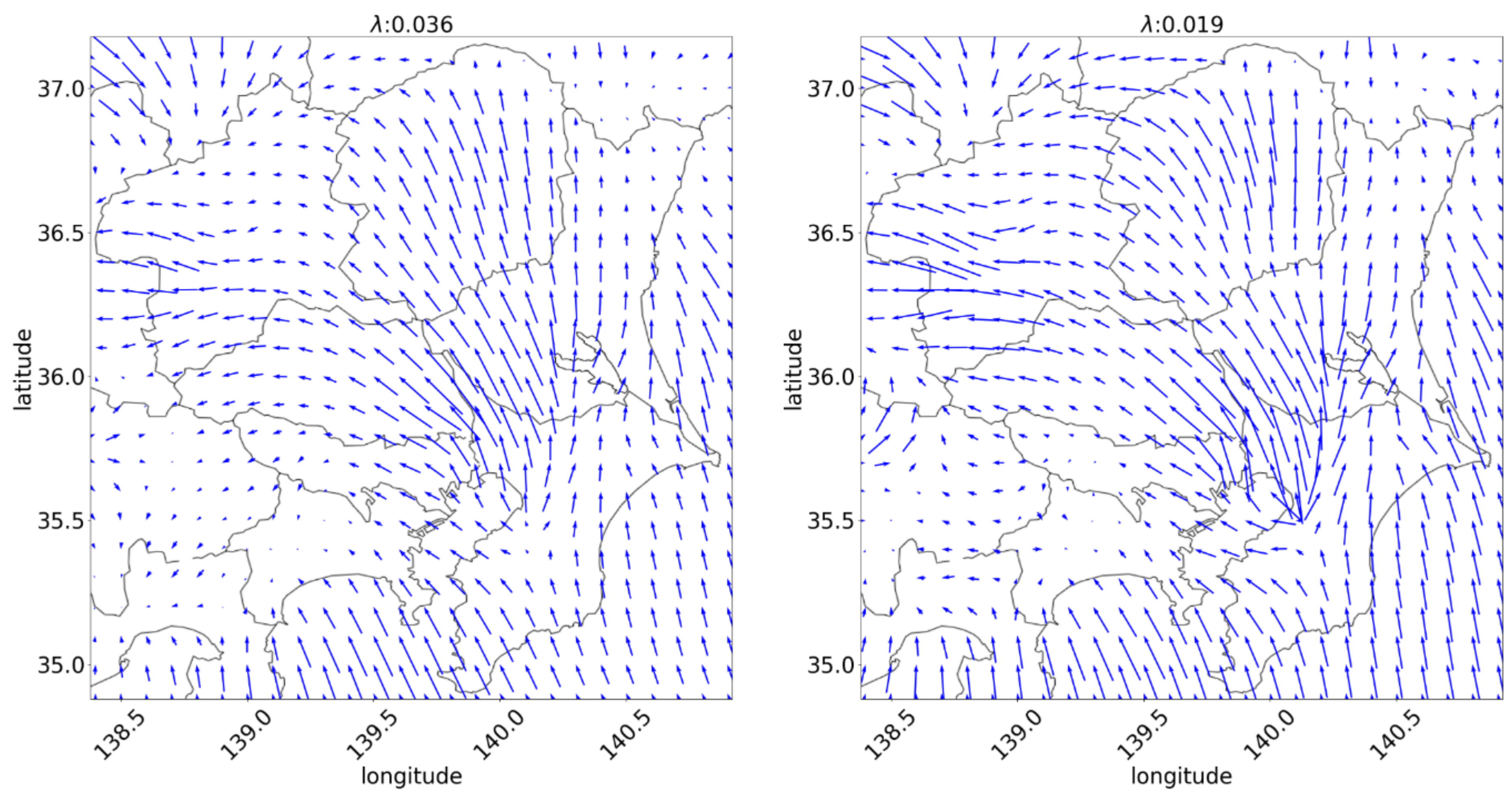
First, an example is presented and explained such that the result of the proposed forecasting is substantially better than that of the persistence forecasting. Figure 13 depicts the box plot of the estimation error at 12:00 on 21 March 2014. It indicates that the proposed forecasting with a large parameter λ does not reduce the error compared to persistence forecasting. Parameter λ is associated with the unity of the vector distribution. Figure 14 depicts three NV distributions at the period, which shows a lump of low NVs in the center that expands, and the spread of NV is non-uniform depending on the direction. In this case, the forecast can be improved with a low λ estimation that considers local motion. Figure 15 is the estimated flow visualization with different λ . It shows that the motion vectors which is yielded with high λ values are too short compared with the practical motions of the lump in Figure 14. However, divergence vector is too large and certain vectors cross each other when λ is too small in Figure 15, which is also considered to be unnatural because weather changes caused mainly by cloud motions are not considered to intersect. On the other hand, the motion vector distributions with λ = 0.019 0.036 have few vector crossings and the fine movement, so they seem to be appropriate.
Another example showing that the result of the proposed forecasting is not better than that of the persistence forecasting is explained. Figure 16 depicts the box plot of the estimation error at 13:00 on 6 September 2013. It indicates that motion estimation does not reduce the forecasting error compared to that of persistence forecasting at 12:30 on 6 September 2013. Figure 17 depicts three NV distributions at the period, which shows the movement of the lumps of the NVs may differ at different times of the period, such as between 11:30 and 12:00, and 12:00 and 12:30. The difference is clearer in the comparison between Figure 18 and Figure 19: Figure 18 shows the distribution of motion vectors from 11:30 to 12:00 calculated using the NV distributions at 11:30 and 12:00 with the best parameter λ = 0.036   and   0.019 , and Figure 19 depicts the distribution of motion vectors from 12:00 to 12:30. Even if the motion vectors in Figure 18 are moved forward in parallel as explained in Figure 4 (such as from vector AB to vector BC), the moved distribution is different from Figure 19. That is to say, the assumption that the movement from t Δ t (11:30) to t (12:00) persists in the period from t (12:00) to t + Δ t (12:30) is not suitable for this period.

4. Conclusions

In this study, a parameter for motion estimation, which was insufficiently discussed in a previous study [22], was investigated for a certain geographic area during drastic change periods. The method proposed in this paper is achieved by normalizing the geographically distributed PV output data, converting them to mesh data, analyzing those motions, generating estimated mesh data from the motions, and converting them into the output of each PV for forecasting. The forecasting was performed using the output data of 5097 PVs located in Japan ( 31 ° 20 39 ° 80 , longitude 129 ° 6′–141 ° 60′) for every 30 min from August 2013 to September 2014. The period when output changed drastically in a certain area within a radius of 15 km in the Kanto region ( latitude   35 ° 78   and   longitude 140 ° 04 ) was extracted to evaluate the forecasting method. The parameters were evaluated from an error distribution of 101 PV units. In comparison with the persistence forecasting, the parameter for motion estimation, which exhibited the smallest error, was able to significantly reduce the error from 23.7% to 10.3%. Motion estimation indicates that the proposed forecasting with a large λ does not reduce the error compared to persistence forecasting. This indicates that low λ estimation improves the prediction by considering local motion when estimating the motion of a wide range of non-uniform NVs.
This result indicates that the parameter presents the best forecast for motion estimation and reduces the error by 56.6% than that of persistence forecasting. The proposed method can effectively forecast for periods when PV output changes drastically.
The following studies should be conducted in the future
  • Correlation between the number of PV data affecting the evaluation area and forecasting accuracy: The proposed forecasting was evaluated using data obtainable in this case. However, the positional relationship and density of PV output in the evaluation area that affect the forecasting accuracy have yet to be investigated. Therefore, it should be considered in the future.
  • Consideration of ensemble learning: It has been reported that ensemble learning, which combines different forecasting models, improves the forecasting accuracy. Therefore, we believe that further improvement of accuracy can be achieved by combining ensemble learning with statistical methodology.

Author Contributions

Conceptualization, J.K.; methodology, J.K. and Y.K.; software, Y.K.; validation, T.K.; formal analysis, T.K.; investigation, T.K. and H.D.T.; resources, J.K.; data curation, T.K., H.D.T., Y.K. and J.K.; ANN, H.Y. and D.K.; writing—original draft preparation, T.K.; writing—review and editing, H.D.T., Y.K., H.Y., D.K. and J.K.; visualization, T.K. and H.D.T.; supervision, J.K. and D.K.; project administration, J.K.; funding acquisition, Y.K. and J.K. All authors have read and agreed to the published version of the manuscript.

Funding

This work was partly supported by JSPS KAKENHI, Grant Number JP21K14150.

Institutional Review Board Statement

Not applicable.

Informed Consent Statement

Not applicable.

Data Availability Statement

Not applicable.

Acknowledgments

The authors thank S. Ogata and M. Ohashi at OMRON Social Solutions Corporation for their invaluable comments. Map data were provided by the Geospatial Information Authority of Japan (https://www.gsi.go.jp/kikaku/index.html) (accessed on 25 January 2022).

Conflicts of Interest

The authors declare no conflict of interest.

References

  1. Adoption of the Paris Agreement—Paris Agreement Text English. Available online: https://unfccc.int/sites/default/files/english_paris_agreement.pdf (accessed on 13 January 2022).
  2. Turner, B. Asian Development Bank Institute. In The Statesman’s Yearbook; Springer Nature: Cham, Switzerland, 2014; p. 75. [Google Scholar] [CrossRef] [Green Version]
  3. GSR2021_Full_Report. Available online: https://www.ren21.net/wp-content/uploads/2019/05/GSR2021_Full_Report.pdf (accessed on 13 January 2022).
  4. Bird, L.; Milligan, M.; Lew, D. Integrating Variable Renewable Energy: Challenges and Solutions; National Renewable Energy Laboratory (NREL): Golden, CO, USA, 2013. [Google Scholar]
  5. Ueckerdt, F.; Brecha, R.; Luderer, G. Analyzing Major Challenges of Wind and Solar Variability in Power Systems. Renew. Energy 2015, 81, 1–10. [Google Scholar] [CrossRef]
  6. Raza, M.Q.; Nadarajah, M.; Ekanayake, C. On recent advances in PV output power forecast. Sol. Energy 2016, 136, 125–144. [Google Scholar] [CrossRef]
  7. Ahmed, R.; Sreeram, V.; Mishra, Y.; Arif, M.D. A review and evaluation of the state-of-the-art in PV solar power forecasting: Techniques and optimization. Renew. Sustain. Energy Rev. 2020, 124, 109792. [Google Scholar] [CrossRef]
  8. Saint-Drenan, Y.M.; Good, G.H.; Braun, M. A probabilistic approach to the estimation of regional photo-voltaic power production. Sol. Energy 2017, 147, 257–276. [Google Scholar] [CrossRef] [Green Version]
  9. Ma, Y.; Lv, Q.; Zhang, R.; Zhang, Y.; Zhu, H.; Yin, W. Short-term photovoltaic power forecasting method based on irradiance correction and error forecasting. Energy Rep. 2021, 7, 5495–5509. [Google Scholar] [CrossRef]
  10. Bacher, P.; Madsen, H.; Nielsen, H.A. Online short-term solar power forecasting. Sol. Energy 2009, 83, 1772–1783. [Google Scholar] [CrossRef] [Green Version]
  11. Reikard, G. Predicting solar radiation at high resolutions: A comparison of time series forecasts. Sol. Energy 2009, 83, 342–349. [Google Scholar] [CrossRef]
  12. Pedro, H.T.C.; Coimbra, C.F.M. Assessment of forecasting techniques for solar power production with no exogenous inputs. Sol. Energy 2012, 86, 2017–2028. [Google Scholar] [CrossRef]
  13. Zhou, H.; Zhang, Y.; Yang, L.; Liu, Q.; Yan, K.; Du, Y. Short-term photovoltaic power forecasting based on long short term memory neural network and attention mechanism. IEEE Access 2019, 7, 78063–78074. [Google Scholar] [CrossRef]
  14. Behera, M.K.; Majumder, I.; Nayak, N. Solar photovoltaic power forecasting using optimized modified extreme learning machine technique. Eng. Sci. Technol. 2018, 21, 428–438. [Google Scholar] [CrossRef]
  15. Alamoudi, R.; Taylan, O.; Aktacir, M.A.; Herrera-viedma, E. Designing a solar photovoltaic system for generating renewable energy of a hospital: Performance analysis and adjustment based on RSM and ANFIS approaches. Mathematics 2021, 9, 2929. [Google Scholar] [CrossRef]
  16. Hammer, A.; Heinemann, D.; Lorenz, E.; Lückehe, B. Short-term forecasting of solar radiation: A statistical approach using satellite data. Sol. Energy 1999, 67, 139–150. [Google Scholar] [CrossRef]
  17. Perez, R.; Kivalov, S.; Schlemmer, J.; Hemker, K.; Renné, D.; Hoff, T.E. Validation of short and medium term operational solar radiation forecasts in the US. Sol. Energy 2010, 84, 2161–2172. [Google Scholar] [CrossRef]
  18. Bright, J.M.; Killinger, S.; Lingfors, D.; Engerer, N.A. Improved satellite-derived PV power nowcasting using real-time power data from reference PV systems. Sol. Energy 2018, 168, 118–139. [Google Scholar] [CrossRef]
  19. Feng, C.; Zhang, J. SolarNet: A sky image-based deep convolutional neural network for intra-hour solar forecasting. Sol. Energy 2020, 204, 71–78. [Google Scholar] [CrossRef]
  20. Chu, Y.; Urquhart, B.; Gohari, S.M.I.; Pedro, H.T.C.; Kleissl, J.; Coimbra, C.F.M. Short-term reforecasting of power output from a 48 MWe solar PV plant. Sol. Energy 2015, 112, 68–77. [Google Scholar] [CrossRef]
  21. Chow, C.W.; Belongie, S.; Kleissl, J. Cloud motion and stability estimation for intra-hour solar forecasting. Sol. Energy 2015, 115, 645–655. [Google Scholar] [CrossRef]
  22. Zhang, J.; Florita, A.; Hodge, B.M.; Lu, S.; Hamann, H.F.; Banunarayanan, V.; Brockway, A.M. A suite of metrics for assessing the performance of solar power forecasting. Sol. Energy 2015, 111, 157–175. [Google Scholar] [CrossRef] [Green Version]
  23. Miyazaki, Y.; Kameda, Y.; Kondoh, J. A power-forecasting method for geographically distributed PV power systems using their previous datasets. Energies 2019, 12, 4815. [Google Scholar] [CrossRef] [Green Version]
  24. Kameda, Y.; Kishi, H.; Ishikawa, T.; Matsuda, I.; Itoh, S. Multi-frame Motion Compensation Using Extrapolated Frame by Optical Flow for Lossless Video Coding. In Proceedings of the 2016 IEEE International Symposium on Signal Processing and Information Technology, ISSPIT 2016, Limassol, Cyprus, 12–14 December 2016; IEEE: Limassol, Cyprus, 2017; pp. 300–304. [Google Scholar]
  25. Horn, B.K.P.; Schunck, B.G. Determining optical flow. Artif. Intell. 1981, 17, 185–203. [Google Scholar] [CrossRef] [Green Version]
  26. Miyazaki, Y.; Kondoh, J.; Kameda, Y. Forecasting System Using Actual Multipoint PV Output; Japan Council for Renewable Energy: Yokohama, Japan, 2018. [Google Scholar]
  27. Interpolate 2-D or 3-D Scattered Data—MATLAB Griddata—MathWorks. Available online: https://jp.mathworks.com/help/matlab/ref/griddata.html?lang=en (accessed on 13 January 2022).
  28. Sawada, Y.; Takahashi, H. Occurrence and mitigation of meso-β-scale precipitation area over the Kanto District in summer. Geogr. Rev. Jap. 2002, 75, 509–528. [Google Scholar] [CrossRef] [Green Version]
  29. Bosch, J.L.; Kleissl, J. Cloud motion vectors from a network of ground sensors in a solar power plant. Sol. Energy 2013, 95, 13–20. [Google Scholar] [CrossRef]
  30. Liu, J.; Fang, W.; Zhang, X.; Yang, C. An improved photovoltaic power forecasting model with the assistance of aerosol index data. IEEE Trans. Sustain. Energy 2015, 6, 434–442. [Google Scholar] [CrossRef]
  31. Tsuchiya, H.D.; Kure, T.; Kodaira, D.; Kondoh, J.; Kameda, Y. Parameter Optimization on Power Output Forecast for Distributed PV Systems Based on Motion Estimation. Preprints 2022, 2022020143. (In Japanese) [Google Scholar] [CrossRef]
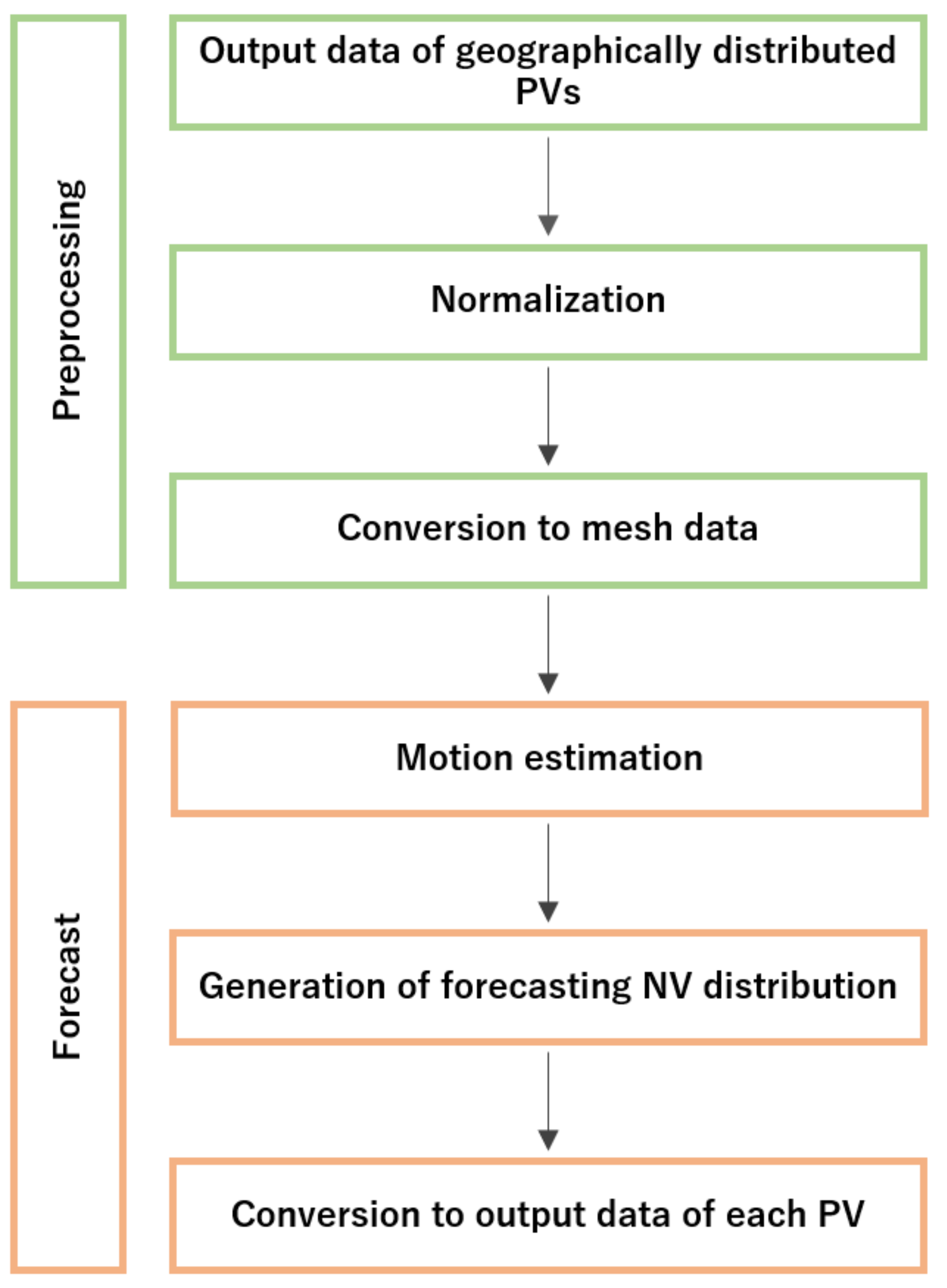
Figure 1. Configuration of the proposed photovoltaic (PV) forecast method.
Energies 15 02855 g001
Figure 2. Concept figure of normalization on 14 July 2014: (a) power generation output lines for 15 days; (b) Normalized values on 14 July 2014.
Energies 15 02855 g002
Figure 3. Concept of conversion to mesh data on 14 July 2014: (a) actual geographical distribution of normalized values (NVs); (b) mesh-arranged geographical distribution converted from (a); (c) interpolated mesh data.
Energies 15 02855 g003
Figure 4. Conceptual figure of motion estimation.
Energies 15 02855 g004
Figure 5. PV systems in the evaluated area.
Energies 15 02855 g005
Figure 6. Sum of the power generation and error of 101 PV systems on 16 March 2014, in the evaluated area: (a) Total output of the evaluation area; (b) APE of the total output in the evaluation area.
Energies 15 02855 g006
Figure 7. Time variation of NV distribution on March 16, 2014, at (a) 11:00, (b) 11:30, and (c) 12:00.
Energies 15 02855 g007
Figure 8. Calculated flow visualizations between 11:00 and 11:30 on 16 March 2014.
Energies 15 02855 g008
Figure 9. Sum of the power generation and error of PV on 5 September 2013, in the evaluated area: (a) Total output of the evaluation area; (b) APE of total output in the evaluation area.
Energies 15 02855 g009
Figure 10. Time variation of NV distribution on 5 September 2013, at (a) 11:30, (b) 12:00, and (c) 12:30.
Energies 15 02855 g010
Figure 11. Calculated flow visualizations between 11:30 and 12:00 on 5 September 2013.
Energies 15 02855 g011
Figure 12. Box plot of the estimation errors in the periods with drastic changes in the output power. The top and bottom of the box indicate the 75th and 25th percentile, respectively.
Energies 15 02855 g012
Figure 13. Box plot of the error distribution at 12:00 on 21 March 2014. The top and bottom of the box indicate the 75th and 25th percentile, respectively.
Energies 15 02855 g013
Figure 14. NV distributions on 21 March 2014, at (a) 11:00, (b) 11:30, and (c) 12:00.
Energies 15 02855 g014
Figure 15. Calculated flow visualizations between 11:00 and 11:30 on 21 March 2014 (improved time).
Energies 15 02855 g015
Figure 16. Box plot of the error distribution at 12:30 on September 6, 2013. The top and bottom of the box indicate the 75th and 25th percentile, respectively.
Energies 15 02855 g016
Figure 17. NV distribution on 6 September 2013, at (a) 11:30, (b) 12:00, and (c) 12:30.
Energies 15 02855 g017
Figure 18. Calculated flow visualizations between 11:30 and 12:00 on 6 September 2013.
Energies 15 02855 g018
Figure 19. Calculated flow visualizations between 12:00 and 12:30 on 6 September 2013.
Energies 15 02855 g019
Table 1. Characteristics of each forecast approach.
ApproachDescriptionEffective Time ScaleReferences
physical approachNWP methods are popular long-term forecast methods for solar irradiance.long-term[8,9]
statistical approachThis includes forecast by autoregressive and artificial intelligence, which are particularly effective in the short-term forecast.very short-term, short-term[10,11,12,13,14,15]
image processing approachThis involves forecasts based on images captured using sensors installed on the ground and artificial satellites.very short-term, short-term[16,17,18,19,20,21]
persistence approachThis approach is effective in very short-term forecasting and is used as a benchmark for the forecast.very short-term[6,12,17]
Table 2. Dataset information.
Period of Dataset1 August 2013–31 July 2014
period of forecasting15 August 2013–31 July 2014
sampling cycle ( Δ t ) obtained from PV30 min
number of PV systems5097
range of the longitude forecasted 31 ° 20 39 ° 80
range of the latitude forecasted129 ° 60′–141 ° 60′
Table 3. Dataset of the evaluated area.
Center Point of the Evaluated Area 35 ° 78 ,   140 ° 04
radius of the evaluated area15 km
number of PVs101
maximum total generation by all PV systems860 kW
time steps of forecasted periods5851
time steps of drastic change periods (extracted)37
Table 4. Error calculated on 16 March 2014.
ParameterPersistenceλ = 1.0λ = 0.52λ = 0.27λ = 0.14λ = 0.071λ = 0.036λ = 0.019λ = 0.0097λ = 0.0050
RMSE [kW]6.9469.7996.8936.4116.1256.9645.4005.4006.1271.105
MAPE [%]0.6500.9390.6520.5780.6490.6480.4940.5630.6140.797
Table 5. Error calculated on 5 September 2013.
ParameterPersistenceλ = 1.0λ = 0.52λ = 0.27λ = 0.14λ = 0.071λ = 0.036λ = 0.019λ = 0.0097λ = 0.0050
RMSE [kW]104.364.4555.9443.5747.3636.9436.6137.7938.1648.20
MAPE [%]9.2305.7794.6313.6293.7222.8813.0613.3623.2774.121
Table 6. Mean, median, and standard deviations of the estimation errors.
ParameterPersistenceArtificial Neural Networkλ = 1.0λ = 0.52λ = 0.27λ = 0.14λ = 0.071λ = 0.036λ = 0.019λ = 0.0097λ = 0.0050
mean [%]23.713.015.515.013.712.811.111.010.310.611.8
medium [%]22.210.213.613.311.510.78.457.837.207.808.87
standard deviations [%]12.510.311.010.910.510.09.5810.29.659.7510.7
Publisher’s Note: MDPI stays neutral with regard to jurisdictional claims in published maps and institutional affiliations.