Optimal Scheduling of Energy Storage System Considering Life-Cycle Degradation Cost Using Reinforcement Learning

Abstract

Recently, due to the ever-increasing global warming effect, the proportion of renewable energy sources in the electric power industry has increased significantly. With the increase in distributed power sources with adjustable outputs, such as energy storage systems (ESSs), it is necessary to define ESS usage standards for an adaptive power transaction plan. However, the life-cycle cost is generally defined in a quadratic formula without considering various factors. In this study, the life-cycle cost for an ESS is defined in detail based on a life assessment model and used for scheduling. The life-cycle cost is affected by four factors: temperature, average state-of-charge (SOC), depth-of-discharge (DOD), and time. In the case of the DOD stress model, the life-cycle cost is expressed as a function of the cycle depth, whose exact value can be determined based on fatigue analysis techniques such as the Rainflow counting algorithm. The optimal scheduling of the ESS is constructed considering the life-cycle cost using a tool based on reinforcement learning. Since the life assessment cannot apply the analytical technique due to the temperature characteristics and time-dependent characteristics of the ESS SOC, the reinforcement learning that derives optimal scheduling is used. The results show that the SOC curve changes with respect to weight. As the weight of life-cycle cost increases, the ESS output and charge/discharge frequency decrease.

1. Introduction

Recently, consumers’ perception of energy has changed due to the development and demonstration of an operating system for regional power grids characterized by VPP and MG. Under the influence of economic factors, such as decreasing installation costs of renewable energy and technological advances, consumers have become energy prosumers who can trade their own electricity through distributed power systems [1,2]. Because the power surplus can be sold to neighbors, the energy flow in the energy market has changed from one-way to two-way. In addition, the existing hierarchical market structure has transformed into a network structure.

With the adoption of distributed energy, the need to establish usage standards is increasing with an increasing use of ESSs. When conducting trading through ESSs, certain usage standards, such as the fuel cost function of the generator, must be considered. The life-cycle cost of the ESS can be considered as one of these standards. As research on the ESS life-cycle, Ref. [3] proposed the total capital cost and life-cycle cost models for ESSs. The cost function was introduced and modeled for the system, and a learning model that can accurately estimate the life-cycle cost based on various battery types was built. Reference [4] proposed an analytical optimization for the capacity and sizing of solar power and ESSs connected to the grid. Ref. [5] studied the efficiency difference between HESS and LESS in an independent microgrid. The constraint variable was set by combining the SOC with the cost function, and the stability of the system was considered in preparation for the surge currents of LIB and LAB. Ref. [6] proposed an ESS life-cycle definition using SOC and SOH models. They established an equation via correlation analysis and introduced a cycle depth variable. Ref. [7] introduced an overall cost evaluation model for ESS and used fuzzy comprehensive evaluation theory to analyze the model, considering basic facility and operating costs. Ref. [8] proposed a life assessment method for ESS in distributed energy systems and established an evaluation method classified into four scenarios. Ref. [9] introduced a P2P energy sharing scheme using ESSs. In their study, scheduling was set to maximize system profits depending on the existence of an ESS. Ref. [10] conducted a comparative study on single/hybrid ESSs to examine stable energy transfer capabilities of these systems. This model considered the charge/discharge rate function of the battery, and data analyses were performed for situations with varying supply and demand. Ref. [11] defined a cycle life model of a battery considering the SOC, DOD, average C-rate, and aging of the lithium-ion battery. A comparative analysis was performed on the battery temperature, output, and resistance values with varying parameters. Ref. [12] introduced an ESS life-cycle cost optimization method through an energy consumer scheduling scheme. The battery life was calculated using the Rainflow counting algorithm for maximizing battery life. Scheduling was configured based on unstable PV and WT output data and the composed ESS life results. Ref. [13] introduced an improvement in the prediction accuracy of lithium-ion batteries. A BP neural network was used to predict the life-cycle cost of the battery, and the weights were set using the DE algorithm. Ref. [14] analyzed the ESS life-cycle cost using various forecasting techniques, such as the RVM and CNN models. Ref. [15] conducted a study on the battery output considering the life-cycle cost of an ESS used in the grid. Their study, conducted on the stability of the system, included measuring the frequency fluctuations over time. Moreover, a scheduling scheme for an ESS used in the auxiliary service market was established. Ref. [16] presented a methodology for the optimal location, selection, and operation of battery energy storage systems (BESSs) and renewable distributed generators in medium- to low-voltage distribution systems. Ref. [17] proposed a new formulation of the battery degradation cost for the optimal scheduling of BESSs. This paper defined a one-cycle battery cost function based on the cycle life curve and an auxiliary state of charge (SOC) that tracks the actual SOC only upon discharge. Ref. [18] proposed a mixed-integer nonlinear programming (MINLP) model for the PV-battery systems which aims to minimize the life-cycle cost (LCC), and solved LCC Problem by a novel two-layer optimization, and Ref. [19] studied the multi-objective operation of BESS in AC distribution systems using a convex reformulation. Ref. [20] proposed a two-stage multi-objective optimal operation scheduling method to improve the operation efficiency and reduce the emission of a solar-power-integrated hybrid ferry with shore-to-ship (S2S) power supply, and Ref. [21] addressed the problem associated with economic dispatch of BESSs in alternating current (AC) distribution networks. Ref. [22] addressed the problem of the optimal operation of BESSs in AC grids from the point of view of multi-objective optimization. Ref. [23] proposed a distributed multi-agent consensus-based control algorithm for multiple BESSs, operating in a microgrid, for fulfilling several objectives, including: SOC trajectories tracking control, economic load dispatch, active and reactive power sharing control, and voltage and frequency regulation. Ref. [24] proposed an optimal BESS scheduling for MGs to solve the stochastic unit commitment problem, considering the uncertainties in renewables and load.

In summary, most previous studies derive their results by defining the life-cycle cost in a quadratic manner or simplifying it. This study aims to define it in detail based on a life-cycle cost assessment method and utilize it for scheduling. Because the defined life-cycle cost cannot be derived analytically and explicitly, a solution is derived using reinforcement learning techniques.

The contributions of this study are as follows:

(1)

By defining the life-cycle cost of an ESS, and deriving and utilizing it for optimal scheduling, prosumers with ESSs can make the best choice between incurring life-cycle costs due to ESS use and profiting from transactions. In addition, because of the active adjustment of prosumers with ESSs, it is possible to reduce the line loss inside a system.

(2)

Through analysis of the trading tendency of flexible prosumers with respect to changes in ESS life-cycle cost weights, prosumers who own an ESS have the choice of participating in P2P energy trading to make profits.

2. Life Degradation Model for ESSs Based on a Life-Cycle Assessment Method

This chapter presents the design of an ESS life-cycle cost metric for prosumer participation in P2P energy trading with ESSs. ESSs can be classified according to the type of battery they use. In this study, lithium-ion batteries, which are commonly used in ESSs, are chosen, and their life-cycle cost is designed. The life-cycle cost was designed based on existing studies related to battery life assessment. The life assessment model consists of four stress models: temperature, average state-of-charge (SOC), depth-of-discharge (DOD), and time Ref. [25].

The degradation ratio of the battery life-cycle is determined by the corresponding stress models, and it can be evaluated using the corresponding degradation ratio. The degradation ratio, four stress models, and the consumption life-cycle ratio are formulated as follows:

$$f_{d,1}=\left[S_{\delta }\left(\delta \right)+S_t\left(t_c\right)\right]S_{\sigma }\left(\sigma \right)S_T\left(T_c\right)$$

(1)

$$S_T\left(T_c\right)=e^{k_T\left(T_c-T_{ref}\right)(\frac{T_{ref}}{T_c})}$$

(2)

$$S_{\sigma }\left(\sigma \right)=e^{k_{\sigma }\left(\sigma -{\sigma }_{ref}\right)}$$

(3)

$$S_{\delta }\left(\delta \right)=k_{\delta ,q1}{\delta }^{k_{\delta ,q2}}$$

(4)

$$S_t\left(t\right)=k_{t}t$$

(5)

$$L=1-{\alpha }_{sei}{e}^{-{\beta }_{sei}{f}_d}-\left(1-{\alpha }_{sei}\right)e^{-f_d}$$

(6)

where $f_d$ is the degradation ratio, and $S_T, S_{\sigma }, S_{\delta }$ are the stresses for temperature, average SOC, and DOD, respectively. $T_c$ is the battery cell temperature, $T_{ref}$ is the reference temperature, and $k_T$ is the temperature stress coefficient. $\sigma$ is the average SOC, ${\sigma }_{ref}$ is the reference average SOC, and $k_{\sigma }$ is the average SOC stress coefficient. $S_t$ is the stress for time, $\delta$ is the cycle depth, and $k_{ \delta ,q1}, k_{ \delta ,q2}$ are the DOD coefficients. $t$ is time, $k_t$ is the time stress coefficient, $L$ is the consumed life-cycle, and ${\alpha }_{sei}, {\beta }_{sei}$ are the solid electrolyte interphase (SEI) film formation coefficients.

In the case of a DOD stress model, various models such as linear, exponential, polynomial, and power are applicable, but the power function is used according to references. Stress models for average SOC and time can be used immediately for life-cycle cost design because they are explicit. The same does not hold for DOD and temperature stress models.

First, in the case of the DOD stress model (4), which is expressed as a function of the cycle depth, the exact value of the cycle depth can be determined through a post evaluation based on fatigue analysis techniques, such as the Rainflow counting algorithm. In the case of the temperature stress model (2), additional analysis is required because a model for the internal battery temperature is required with respect to the output ESS. Therefore, additional design stages for these two models are required. The model for temperature is designed by analyzing the relationship between battery output and temperature using the thermoelectric model of the battery. Furthermore, for the DOD model in this case, an approximation that considers one charge or discharge of the battery as a half cycle is assumed.

2.1. Temperature Stress Model Formulation

A thermoelectric model is used as the temperature stress model, which is categorized into two types: an electric circuit model and a thermal model Refs. [26,27,28,29].

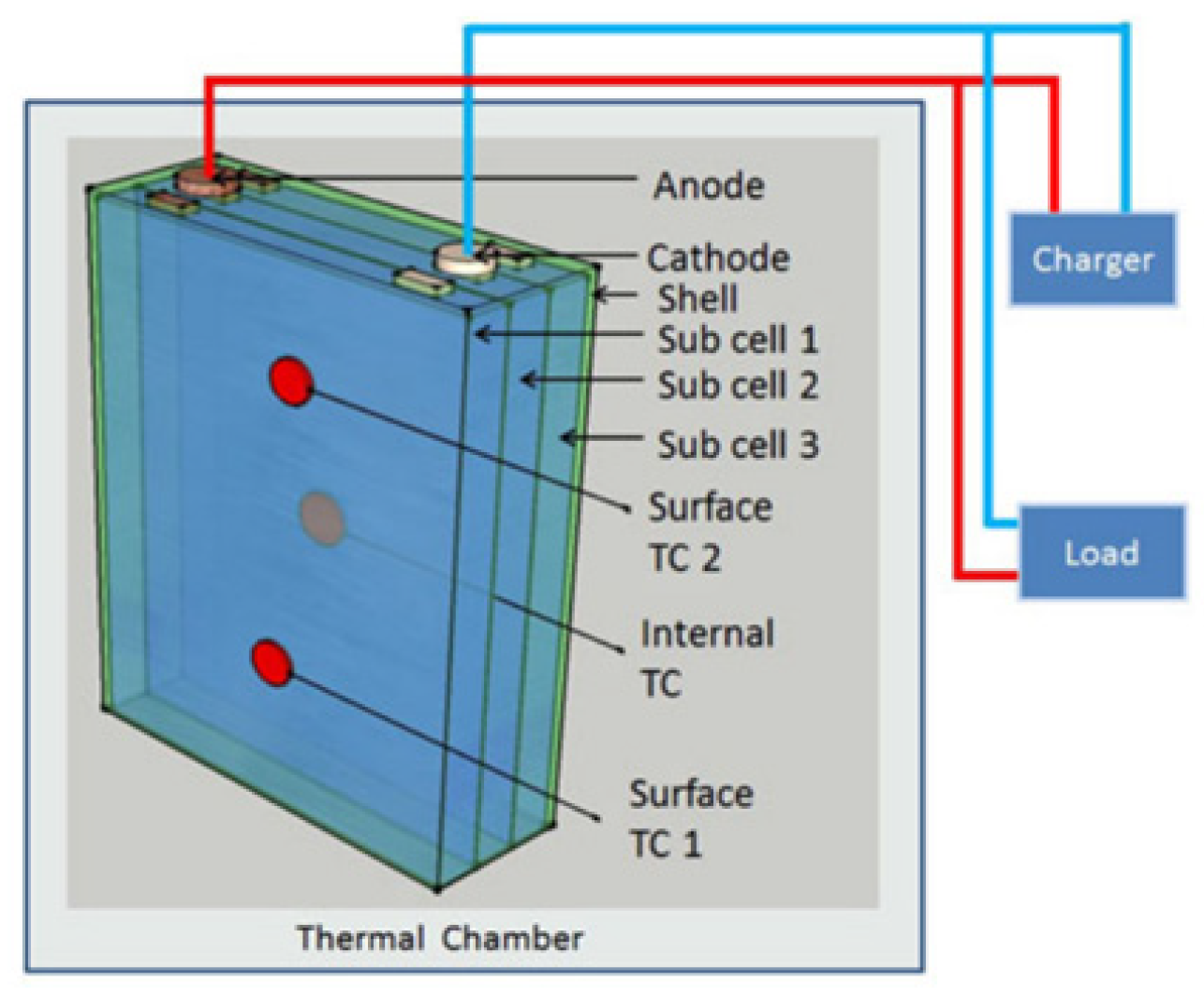
2.1.1. Electric Circuit Model

The electric circuit model of the battery used in the temperature stress model is shown in Figure 1 Ref. [28]. The open circuit voltage (OCV) can be expressed as a function of the SOC and internal temperature of the battery. OCV, characteristically, rises during charging and falls during discharging, and this tendency varies according to SOC. The internal resistance $R_{in}$ can also be expressed as a function of SOC and temperature. The RC network located to the right of the internal resistance is a secondary model and represents the diffusion resistance and capacitance. $R_1$ and $C_1$ are related to the charge transfer processes occurring in the middle frequency range, whereas $R_2$ and $C_2$ are responsible for reproducing the diffusion processes. $V_h$ is an additional voltage component caused by the hysteresis characteristics of the RC network, which refers to the fluctuations on the open voltage during charge/discharge. This component is ignored, assuming its effect is relatively small. Moreover, the corresponding model for life-cycle cost analysis does not require detailed dynamic characteristics of the battery.

The function for the SOC of the OCV (7) is based on the parameters listed in

Table 1. Battery OCV curve parameters.

Parameter	a	b	c	d
Value	3.263	0.02451	−0.2297	−7.666

.

$$\mathrm{OCV}=f\left(\mathrm{SOC}\right)=a{e}^{\left(b·\mathrm{SOC}\right)}+c{e}^{\left(d·\mathrm{SOC}\right)}$$

(7)

Regarding the effect of temperature on the OCV, Equation (8) shows the correlation between the OCV bias component and temperature. It can be expressed as a polynomial with the following related parameters in

Table 2. Correlation parameters between OCV bias component and temperature/SOC.

Parameter	$\mathit{p}\mathit{00}$	$\mathit{p}\mathit{10}$	$\mathit{p}\mathit{01}$	$\mathit{p}\mathit{20}$
Value	−0.001202	0.2458	$8.558\times {10}^{-5}$	−1.248
Parameter	$\mathit{p}\mathit{11}$	$\mathit{p}\mathit{02}$	$\mathit{p}\mathit{30}$	$\mathit{p}\mathit{21}$
Value	−0.007113	$1.552\times {10}^{-5}$	2.328	0.03044
Parameter	$\mathit{p}\mathit{12}$	$\mathit{p}\mathit{40}$	$\mathit{p}\mathit{31}$	$\mathit{p}\mathit{22}$
Value	$-1.063\times {10}^{-5}$	−1.899	−0.04233	$-7.069\times {10}^{-5}$
Parameter	$\mathit{p}\mathit{50}$	$\mathit{p}\mathit{41}$	$\mathit{p}\mathit{32}$
Value	0.569	0.01919	$8.263\times {10}^{-5}$

:

$$\begin{array}{c}{b}_{\mathrm{OCV}}=g\left(\mathrm{SOC},T_{in}\right)\\ =p00+p10·\mathrm{SOC}+p01·T_{in}+p20·{\mathrm{SOC}}^2+p11·\mathrm{SOC}·T_{in}+p02·{T_{in}}^2+p31·{\mathrm{SOC}}^3\\ +p21·{\mathrm{SOC}}^2·T_{in}+p12·\mathrm{SOC}·{T_{in}}^2+p40·{\mathrm{SOC}}^4+p31·{\mathrm{SOC}}^3·T_{in}+p22·{\mathrm{SOC}}^2·{T_{in}}^2\\ +p50·{\mathrm{SOC}}^5+p41·{\mathrm{SOC}}^4·T_{in}+p32·{\mathrm{SOC}}^3·{T_{in}}^2\end{array}$$

(8)

Finally, the open circuit model is constructed as a linear sum of the OCV model for SOC in Equation (9).

$$\mathrm{OCV}=f\left(\mathrm{SOC},T_{in}\right)=f\left(\mathrm{SOC}\right)+g\left(\mathrm{SOC},T_{in}\right)$$

(9)

The SOC is updated according to the output current, whose unit can be set as % (or p.u.). The sign of the discharge current was set to positive. The discrete equation can be described as:

$$\mathrm{SOC}\left(k\right)=\mathrm{SOC}\left(k-1\right)-\frac{i\left(k-1\right)}{C_n}\frac{T_s}{3600}$$

(10)

where $T_s$ is the sampling time (unit: second [s]), $C_n$ is the battery capacity (unit: Ampere hour [Ah]), $i$ is the output current, and $k$ is a time index.

The internal resistance is also configured as a function of the internal temperature and SOC, similar to the OCV. However, the internal resistance remains constant without significant changes over the general battery SOC usage period and is dominantly affected by the internal temperature Ref. [19]. Therefore, the internal resistance is expressed as a function of the internal temperature with the battery internal resistance curve parameters in

Table 3. Battery internal resistance curve parameters.

Parameter	a	b	c	d
Value	0.0003448	−0.2954	0.01771	−0.008504

and formulated as follows:

$$R_{in}=f_R\left(T_{in}\right)=a{e}^{b{T}_{in}}+c{e}^{d{T}_{in}}$$

(11)

The relationship between voltage, resistance, and current in an RC network can be represented as

$$v_1\left(k\right)=a_1{v}_1\left(k-1\right)+b_{1}i\left(k-1\right), a_1=e^{-(\frac{T_s}{R_1{C}_1})}, b_1=R_1\left(1-a_1\right)$$

(12)

$$v_2\left(k\right)=a_2{v}_2\left(k-1\right)+b_{2}i\left(k-1\right), a_2=e^{-(\frac{T_s}{R_2{C}_2})}, b_2=R_2\left(1-a_2\right)$$

(13)

where $T_s$ is the sampling time, and $k$ is the discrete time index. The second network time constant does not change Ref. [28]; thus, what remains to be estimated are the resistance and time constant of the first RC network and the resistance of the second RC network. If $R_1$ and ${\tau }_1$ are known, then using the time constant relational expression ($\tau =RC$) $C_1$ can be calculated, and $C_2$ can be calculated in a similar manner if $R_2$ and ${\tau }_2$ are known. Network resistances are based on a polynomial model, whereas the first time constant is based on an exponential equation. The equations are stated below and parameters are shown in

Table 4. Correlation parameters between RC Network $R_1$ and SOC/internal temperature.

Parameter	$\mathit{p}\mathit{00}$	$\mathit{p}\mathit{10}$	$\mathit{p}\mathit{01}$	$\mathit{p}\mathit{20}$
Value	0.04375	−0.05367	$-0.000974$	0.01182
Parameter	$\mathit{p}\mathit{11}$	$\mathit{p}\mathit{02}$	$\mathit{p}\mathit{21}$	$\mathit{p}\mathit{12}$
Value	0.0005085	$7.661\times {10}^{-6}$	0.0004819	$-6.957\times {10}^{-6}$
Parameter	$\mathit{p}\mathit{03}$
Value	$1.993\times {10}^{-8}$

,

Table 5. Correlation parameters between RC Network $R_2$ and SOC/internal temperature.

Parameter	$\mathit{p}\mathit{00}$	$\mathit{p}\mathit{10}$	$\mathit{p}\mathit{01}$	$\mathit{p}\mathit{20}$
Value	0.05018	−0.1373	$-0.002979$	0.1224
Parameter	$\mathit{p}\mathit{11}$	$\mathit{p}\mathit{02}$	$\mathit{p}\mathit{30}$	$\mathit{p}\mathit{21}$
Value	0.005049	$0.0001103$	−0.02099	−0.001888
Parameter	$\mathit{p}\mathit{12}$	$\mathit{p}\mathit{03}$	$\mathit{p}\mathit{31}$	$\mathit{p}\mathit{22}$
Value	$-9.877\times {10}^{-5}$	$-2.118\times {10}^{-6}$	−0.001455	$5.704\times {10}^{-5}$
Parameter	$\mathit{p}\mathit{13}$	$\mathit{p}\mathit{04}$
Value	$2.744\times {10}^{-7}$	$1.708\times {10}^{-8}$

and

Table 6. Correlation parameter between RC Network first time constant and SOC.

Parameter	a	b
Value	53.99	−1.573

.

$$\begin{array}{cc}{R}_1=f_{R_1}\left(\mathrm{SOC},T_{in}\right)& \\ & =p00+p10·\mathrm{SOC}+p01·T_{in}+p20·{\mathrm{SOC}}^2+p11·\mathrm{SOC}·T_{in}\\ & +p02·{T_{in}}^2+p21·{\mathrm{SOC}}^2·T_{in}+p12·\mathrm{SOC}·{T_{in}}^2+p03·{T_{in}}^3\end{array}$$

(14)

$$\begin{array}{cc}{R}_2=f_{R_2}\left(\mathrm{SOC},T_{in}\right)& \\ & =p00+p10·\mathrm{SOC}+p01·T_{in}+p20·{\mathrm{SOC}}^2+p11·\mathrm{SOC}·T_{in}\\ & +p02·{T_{in}}^2+p30·{\mathrm{SOC}}^3+p21·{\mathrm{SOC}}^2·T_{in}+p12·\mathrm{SOC}\\ & ·{T_{in}}^2+p03·{T_{in}}^3+p31·{\mathrm{SOC}}^3·T_{in}+p22·{\mathrm{SOC}}^2·{T_{in}}^2+p13\\ & ·\mathrm{SOC}·{T_{in}}^3+p04·{T_{in}}^4\end{array}$$

(15)

$${\tau }_1=f_{{\tau }_1}\left(\mathrm{SOC}\right)=a{e}^{b·\mathrm{SOC}}$$

(16)

2.1.2. Lumped Thermal Model

As shown in Figure 2, the battery thermal model is affected by the temperature values at three points: the cell inside the battery shell, shell surrounding it, and environment Ref. [19].

Therefore, the battery thermal model can be modeled in two ways: the heat generation that occurs inside the battery and heat transfer from the inside to the battery shell and from the shell to the environment. In general, heat generated by the cell is considered only as the heat generated by the internal resistance.

However, the heat generated due to the overpotential of the RC network and entropy change also need to be considered. The total heat generated by the cell is given by

$$Q=R_{in}{i}^2+v_{1}i+v_{2}i+i\times T_{in}\frac{d\mathrm{OCV}}{d{T}_{in}}$$

(17)

In general, the heat transfer in and out of a battery includes three mechanisms: conduction, convection, and radiation. Before modeling the heat transfer, both the battery shell temperature and internal temperature must be uniform, and the thermal characteristics must also be uniformly distributed inside the battery. Only the heat conduction between the inside and shell of the battery and between the shell and environment is considered. The heat transfer model is expressed as follows:

$$C_{q1}\frac{d{T}_{in}}{dt}=Q-k_1\left(T_{in}-T_{sh}\right)$$

(18)

$$C_{q2}\frac{d{T}_{sh}}{dt}=k_1\left(T_{in}-T_{sh}\right)-k_2\left(T_{sh}-T_{amb}\right)$$

(19)

where $T_{in}$ is the battery internal temperature, $T_{sh}$ is the battery shell temperature, and $T_{amb}$ is the ambient temperature. $C_{q1}$ and $C_{q2}$ are the internal and shell thermal capacities of the battery, respectively, and $k_1$ and $k_2$ are the heat conduction coefficients between the battery internal and the shell, and between the battery shell and the ambience, respectively. Because Equations (18) and (19) are continuous, they are discretized as follows:

$$C_{q1}\frac{z-1}{T_s}{T}_{in}=Q-k_1\left(T_{in}-T_{sh}\right)$$

(20)

$$C_{q2}\frac{z-1}{T_s}{T}_{in}=k_1\left(T_{in}-T_{sh}\right)-k_2\left(T_{sh}-T_{amb}\right)$$

(21)

Finally, the formulae for the internal temperature and shell temperature are as given by

$$T_{in}\left(k+1\right)=\frac{1-T_s{k}_1}{C_{q1}}{T}_{in}\left(k\right)+\frac{T_s{k}_1}{C_{q1}}{T}_{sh}\left(k\right)+\frac{T_{s}Q\left(k\right)}{C_{q1}}$$

(22)

$$T_{sh}\left(k+1\right)=\frac{T_s{k}_1}{C_{q2}}{T}_{in}\left(k\right)+\frac{1-T_s\left(k_1+k_2\right)}{C_{q2}}{T}_{sh}\left(k\right)+\frac{T_s{k}_2{T}_{amb}}{C_{q2}}$$

(23)

The heat capacity coefficients and internal heat capacity are constant. The heat capacity coefficient $k_2$ used in this model has time-varying characteristics; and the following relation holds Ref. [28]:

$$k_2=k_{21}+k_{22}\left(T_{sh}-T_{amb}\right)$$

(24)

The $k_2$ certainly depends on the heat dissipation condition, such as cooling wind speed and temperature. $k_2$ also increases with this temperature gradient $T_{sh}-T_{amb}$. To take this effect into consideration, two cases are compared here: Constants $k_{21}$ of $k_2$ and time-varying $k_{22}$ of $k_2$.

2.1.3. Coupled Thermoelectric Model

By combining the two previously defined thermal/electrical models into one,

$$x\left(k+1\right)=Ax\left(k\right)+B\left(k\right)$$

(25)

$$v\left(k\right)=\mathrm{OCV}\left(k\right)+v_1\left(k\right)+v_2\left(k\right)-i\left(k\right)R_{in}$$

(26)

where,

$$x\left(k\right)={\left[\mathrm{SOC}\left(k\right), v_1\left(k\right), v_2\left(k\right), T_{in}\left(k\right), T_{sh}\left(k\right)\right]}^T$$

$$A=\left[\begin{array}{cc}\begin{array}{ccc}1& 0& 0\\ 0& a_1& 0\\ 0& 0& a_2\end{array}\hfill & \begin{array}{cc}0& 0\\ 0& 0\\ 0& 0\end{array}\\ \begin{array}{ccc}0& 0& 0\\ 0& 0& 0\end{array}\hfill & \begin{array}{cc}1-k_1\frac{T_s}{C_{q1}}& k_1\frac{T_s}{C_{q1}}\\ k_1\frac{T_s}{C_{q2}}& 1-\left(k_1+k_2\right)\frac{T_s}{C_{q2}}\end{array}\end{array}\right]$$

$$B\left(k\right)={\left[-i\left(k\right)\frac{T_s}{C_n},-b_{1}i\left(k\right),-b_{2}i\left(k\right), Q\left(k\right)\frac{T_s}{C_{q1}}, k_2{T}_{amb}\frac{T_s}{C_{q2}}\right]}^T$$

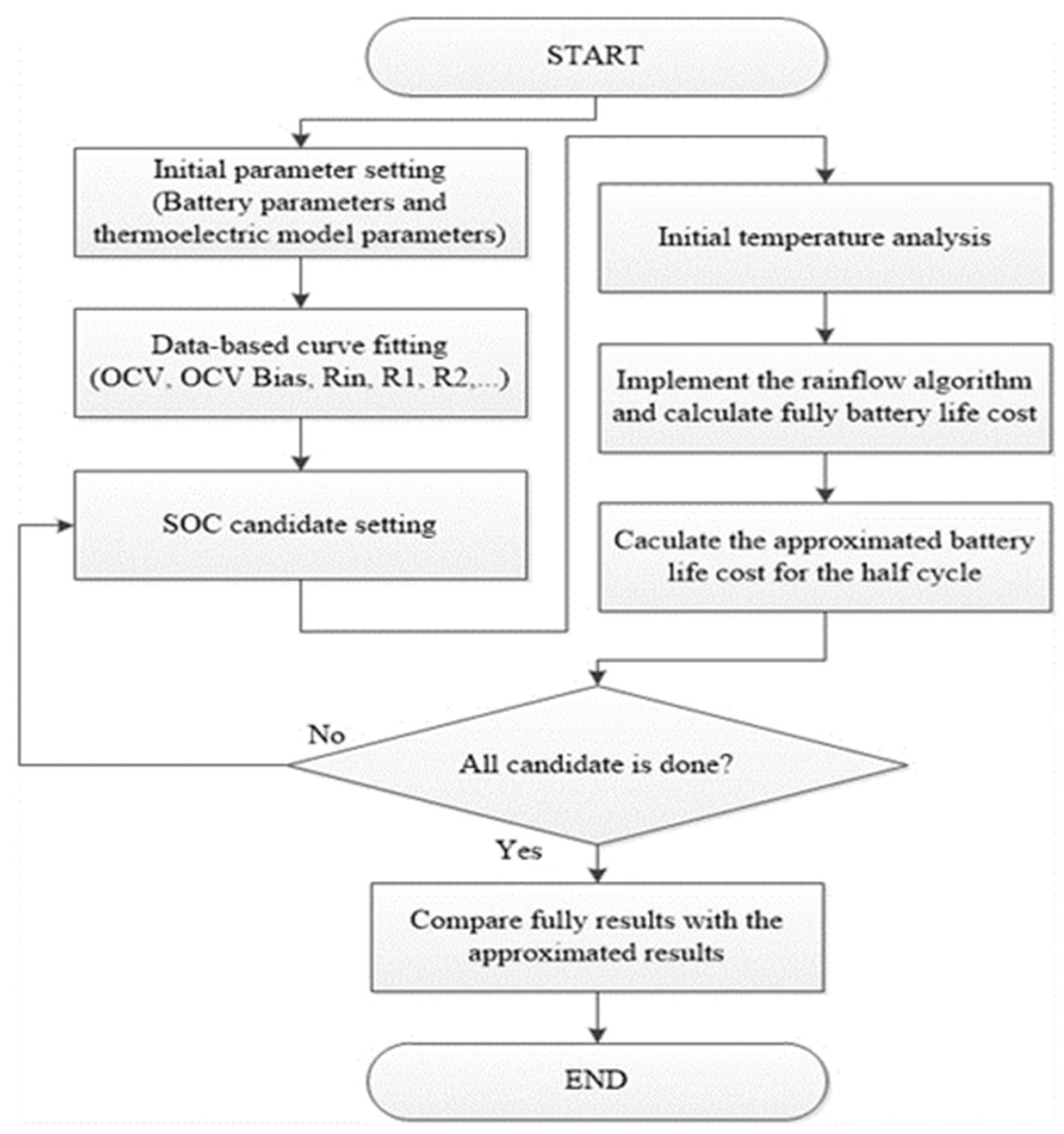
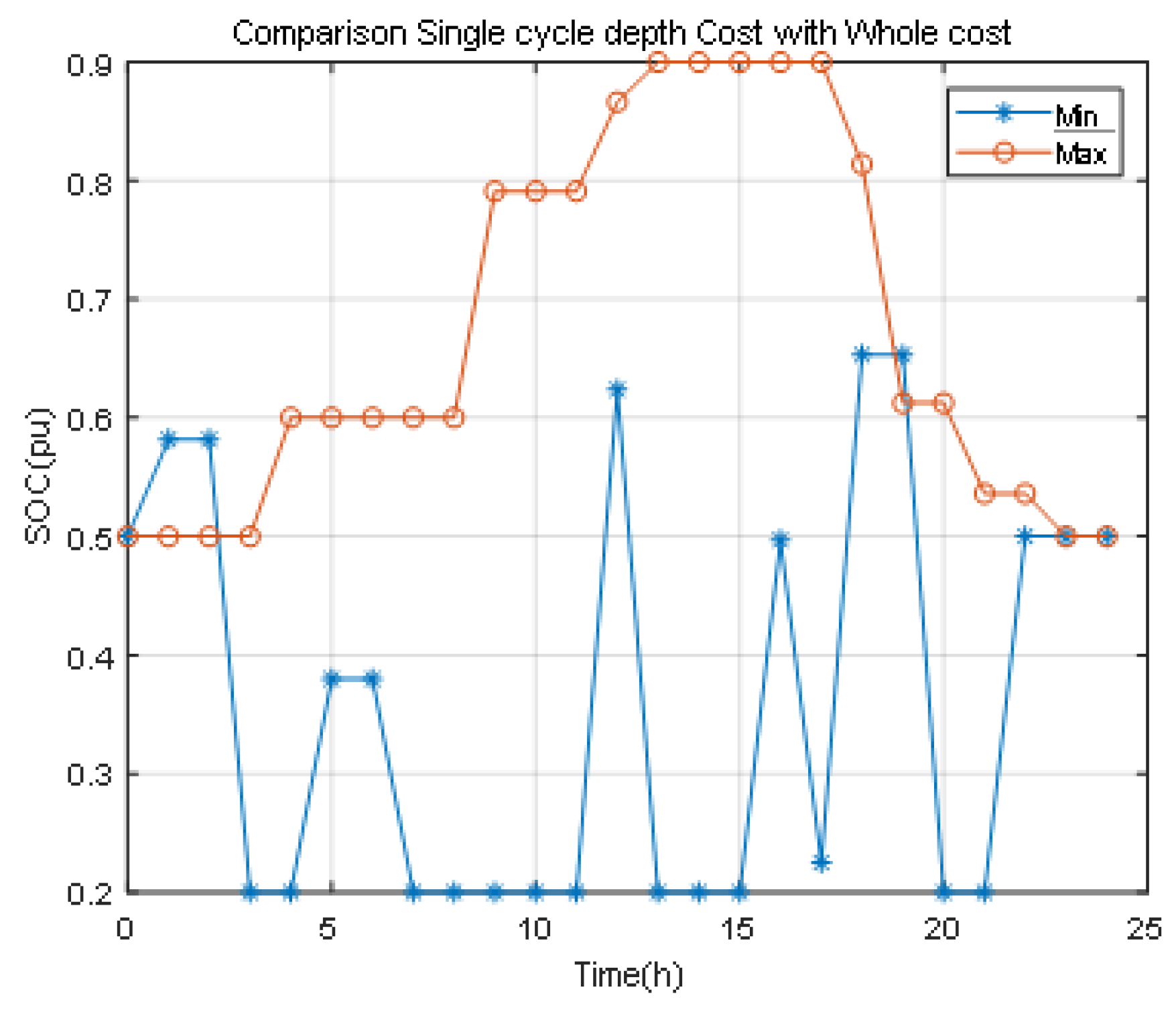
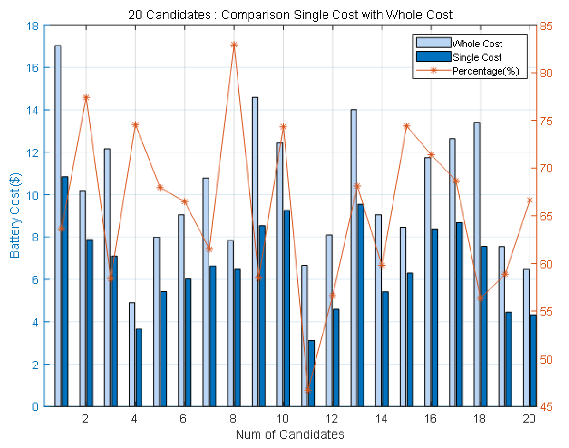
2.2. Cycle Depth Stress Model Formulation

The cycle depth is derived after fatigue analysis using the Rainflow counting algorithm, as mentioned earlier in the study related to the life-cycle cost evaluation of the ESS. Therefore, it is impossible to determine the cycle depth before scheduling is configured. The first step in solving this problem is deriving it through dynamic programming when composing the ESS schedule. However, in dynamic programming, a cost or reward should be calculated at the transition time between states. It is necessary to define a state, which can be the SOC of the ESS. However, because SOC is a continuous variable, it cannot be determined discretely; however, the state can be defined by dividing it into a specific unit as a simplification to reduce the burden of calculation. For example, if the state is defined in units of 0.1, when the minimum SOC is 0.1 and the maximum SOC is 0.9, nine states can be defined in one time period (Stage). When the total schedule interval is T, the number of cases composed by states is $9^{T-1}$. This refers to the number of cases when searching for a path from the first to the last stage in the dynamic plan. That is, the computational power required to search for an optimal point is quite large. To solve this problem, a reinforcement learning-based approach is introduced, and the cycle depth to be used in this approach is approximated. Therefore, for the cycle depth, the same half cycle was applied for all charging/discharging cycles. To check whether this approximation is appropriate, we created a random SOC candidate group and compared the difference between the complete and approximate life-cycle cost analysis results.

Figure 3 shows a flowchart depicting this process. Figure 4 shows the SOC graph where the difference between the two results is maximum and minimum when the life-cycle costs for the approximated and total cycle depths are calculated. As a result, when charging and discharging are repeatedly performed, the difference between the two life costs is small, as shown in the blue graph, whereas when charging and discharging are sequentially performed in one large cycle depth, the difference is the largest.

Figure 5 shows the approximated cycle depth for 20 candidates and the life-cycle cost for the total cycle depth, as well as the ratio between the two life-cycle costs. Although there is a difference in the ratio for each candidate group, we confirmed that even if the life-cycle cost is calculated using the approximated cycle depth, the effect could be similar to the lifetime cost calculated using the total cycle depth. When the life-cycle cost is included in the actual objective function, it may be lower than the actual expected life-cycle cost owing to the approximated cycle depth. However, this can be avoided because the life-cycle cost is used for weight and not directly converted into an actual financial cost.

2.3. ESS Life-Cycle Cost Formulation

Considering the temperature and DOD stress models, the ESS life-cycle cost can be expressed as

$$f_d=0.5\left[S_{\delta }\left(\delta \right)+S_t\left(t_c\right)\right]S_{\sigma }\left(\sigma \right)S_T\left(T_c\right)$$

(27)

$$S_T\left(T_c\right)=e^{k_T\left(T_c-T_{ref}\right)(\frac{T_{ref}}{T_c})}$$

(28)

$$T_c=f\left(P_{bat}\right)$$

(29)

$$S_{\sigma }\left(\sigma \right)=e^{k_{\sigma }\left({\sigma }^t+\frac{\eta P_{bat}}{2C_{ESS}}-{\sigma }_{ref}\right)}$$

(30)

$$S_{\delta }\left(\delta \right)=k_{\delta ,q1}{\left(\frac{\eta P_{bat}}{C_{ESS}}\right)}^{k_{\delta ,q2}}$$

(31)

$$S_t\left(t\right)=k_{t}t$$

(32)

$$L=1-{\alpha }_{sei}{e}^{-{\beta }_{sei}{f}_d}-\left(1-{\alpha }_{sei}\right)e^{-f_d}$$

(33)

where $P_{bat}$ and $C_{ESS}$ are the output and capacity of the ESS, respectively. $\eta$ is the ESS charging/discharging efficiency, and ${\sigma }^t$ is the SOC at time $t$. Because the consumed life-cycle $L$ presented in Equation (33) is a cumulative expression of the battery aging, the difference in $L$ values reflects the actual shortened lifespan. For example, if the life-cycle $L_1$ consumed on the first day and life-cycle $L_2$ consumed on the second day are determined through life assessment, the actual life-cycle consumed on the second day becomes $L_2-L_1$. If this is applied in the dynamic programming method mentioned above, complex calculations, such as the number of cases for the path by the SOC state, must proceed. Therefore, to maintain the tendency of the life-cycle cost and lower the computational complexity, the initially consumed life-cycle value is initialized at 0. The calculation complexity can be reduced using only the degradation ratio and life-cycle cost.

Finally, the life-cycle cost of the ESS is treated as a concept of depreciation cost by multiplying the investment cost for the battery, as shown in Equation (34).

$$f_{bat}\left(t\right)=I{n}_{bat}\times L\left(t\right)$$

(34)

$f_{bat}$ is the life-cycle cost, and $I{n}_{bat}$ is the investment cost for the battery. The DOD stress model can be solved analytically through half-cycle approximation. However, the temperature stress model cannot be directly used for optimization problems because it is derived through dynamic characteristic analysis. Therefore, this problem is solved through a reinforcement learning approach.

3. ESS Scheduling Formulation Considering the Life-Cycle Cost

The basic optimization problem regarding a prosumer who owns an ESS is the summation of the cost of electricity purchased from the grid and life-cycle cost of the ESS, which can be expressed as follows:

$$f_{pros}^{ESS}={\displaystyle \sum }_{t=1}^T[{\omega }_{ESS}{I}_{ESS}{L}_{ESS}^t+\left(1-{\omega }_{ESS}\right){\pi }_{grid}^t{P}_{grid}^t]$$

(35)

$$P_{grid}^t+P_{dch}^t-P_{ch}^t=P_{load}^t-P_{PV}^t$$

(36)

$${\mathrm{SOC}}^{t+1}={\mathrm{SOC}}^t+\frac{({\eta }_{eff}{P}_{ch}^t-\left(\frac{P_{dch}^t}{{\eta }_{ef}}\right)) }{C_{ESS}}\Delta t$$

(37)

$${\mathrm{SOC}}^0={\mathrm{SOC}}_{init}$$

(38)

$${\mathrm{SOC}}^t={\mathrm{SOC}}_{end}$$

(39)

$$L_{ESS}^t=1-{\alpha }_{sei}{e}^{-{\beta }_{sei}{f}_d^t}-\left(1-{\alpha }_{sei}\right)e^{-f_d^t}$$

(40)

$$f_d^t=F\left(S_{\delta }^t, S_t^t, S_{\sigma }^t, S_T^t\right)=0.5\left(S_{\delta }^t+S_t^t\right) S_{\sigma }^t S_T^t$$

(41)

$$S_{\delta }^t=k_{\delta ,q1}{\left({\delta }^t\right)}^{k_{\delta ,q2}}$$

(42)

$${\delta }^t=\frac{{\eta }_{eff}{P}_{ch}^t+P_{dch}^t/{\eta }_{dch}}{C_{ESS}}$$

(43)

$$S_t^t=k_{t}t$$

(44)

$$S_{\sigma }^t=e^{k_{\sigma }\left({\sigma }^t-{\sigma }_{ref}\right)}$$

(45)

$${\sigma }^t=\frac{\left|{\mathrm{SOC}}^{t+1}+{\mathrm{SOC}}^t \right|}{2}=\frac{2{\mathrm{SOC}}^t+{\eta }_{eff}{P}_{ch}^t+P_{dch}^t/{\eta }_{dch}}{2C_{ESS}}$$

(46)

$$S_T^t=e^{k_T\left(T_c^t-T_{ref}\right)(\frac{T_{ref}}{T_c^t})}$$

(47)

$$0\le P_{dch}^t\le P_{bat}^{rated}$$

(48)

$$0\le P_{ch}^t\le P_{bat}^{rated}$$

(49)

$${\mathrm{SOC}}^{\mathit{min}}\le {\mathrm{SOC}}^t\le {\mathrm{SOC}}^{max}$$

(50)

$$0\le P_{grid}^t\le P_{grid}^{max}$$

(51)

In (35), weights are applied to both the ESS life-cycle cost and system purchase cost to reflect the subjective preference of the ESS operator regarding the life-cycle cost. The larger this weight is, the larger the ESS life-cycle is, which is reduced when operating the ESS, whereas the system purchase cost is considered relatively low. Regarding this problem, the state and stage for the ESS SOC are defined as shown in Figure 6, and a reward table for state transition is constructed for reinforcement learning.

Figure 7 shows a flowchart for deriving a solution that applies reinforcement learning to the optimization problem considering the life-cycle cost of the ESS. Figure 8 and Figure 9 show examples of internal reward tables for reinforcement learning. Because this problem is a cost minimization problem, the cost value is treated with a negative sign.

All problems subject to reinforcement learning can be expressed as a Markov decision process (MDP) model, and this MDP is based on the Markov process (MP). The purpose of reinforcement learning is to solve the Bellman Equations below.

$$V_{\pi }\left(s\right)={{\displaystyle \sum }}_{a\in \hat{A}}\pi \left(\left.a\right|s\right)Q_{\pi }\left(s,a\right)$$

(52)

$$V_{\pi }\left(s\right)={{\displaystyle \sum }}_{a\in \widehat{A}}\pi \left(\left.a\right|s\right)(R_s^a+\gamma {{\displaystyle \sum }}_{s^{\prime }\in \widehat{S}}{P}_{s{s}^{\prime }}^a{V}_{\pi }\left(s^{\prime }\right))$$

(53)

$$Q_{\pi }\left(s,a\right)=R_s^a+\gamma {{\displaystyle \sum }}_{s^{\prime }\in \widehat{S}}{P}_{s{s}^{\prime }}^a{{\displaystyle \sum }}_{a^{\prime }\in \widehat{A}}\pi \left(\left.a^{\prime }\right|s^{\prime }\right)Q_{\pi }\left(s^{\prime }{a}^{\prime }\right)$$

(54)

$$V_{\pi }^{*}\left(s\right)=\max \left(V_{\pi }\left(s\right)\right) , Q_{\pi }^{*}\left(s,a\right)=\max \left(Q_{\pi }\left(s,a\right)\right)$$

(55)

$$Q\left(s,a\right)=Q\left(s,a\right)+{\alpha }_{lr}\Delta Q$$

(56)

(52)–(54) are the Bellman Expectation Equations. If the optimal value of $Q$ is found as in (55), the action state $a^{*}$ can be obtained and ${\pi }^{*}$ can be obtained accordingly. In (54), $R_s^a$, the reward of action $a$ in state $s$ is the sum of the negative values of the cost for energy consumption and the life-cycle cost as shown in Figure 9. $P_{s{s}^{\prime }}^a$, the probability of transition from s to $s^{\prime }$ is set to 1 in this problem. For example, when SOC 0.5 is state $s$ and 0.4 is $s^{\prime }$, the action is a discharge corresponding to the amount of energy for SOC 0.1 which is a difference. As a result, when the action of discharging from SOC 0.5 to 0.4 is selected, the probability of the transition becomes 1 because another state cannot exist according to this action. The discount factor $\gamma$ is used to evaluate future rewards at the point in time. When determining the optimal scheduling, the $\gamma$ is set to 1 in this problem because the reward is not discounted. The function approximator solves the problem by finding the value function value in the reverse order from the final state through (54) and updating the Q(s,a) value as shown in (56).

4. Simulation Results

The MDP object is defined through the configured table, and the problem is solved using the reinforcement learning toolbox of MATLAB 2019a. Figure 10 shows the battery open circuit voltage fitting curve and Figure 11 shows the bias model for temperature and SOC. Figure 12 shows the battery internal resistance/temperature curve and Figure 13 and Figure 14 show RC network R curves and surface with respect to SOC/Internal Temperature.

Table 7. Setting parameters for the Q-learning agent and training options.

Q-Learning Agent Options	Learning Rate	Epsilon Greedy Exploration Probability		Epsilon Decay
Parameter value	0.1	0.9		0.01
Trading Options	Max steps per episode		Max episodes
Parameter Value	20,000		20,000

shows the settings for the agent and training options.

For the optimal scheduling of ESS, the power system’s architecture is shown as Figure 15a and is behind the meter. Figure 15b shows the load power curve and PV output curve. In the case of the ESS used in this paper, the load and PV were modeled in the behind the meter (BTM) method. Figure 16 demonstrates the process of finding the path to the SOC through reinforcement learning.

By changing the weight for the life-cycle cost through reinforcement learning, we checked whether the effect of the life-cycle cost is reflected in the ESS SOC results in Figure 17.

The results in Figure 17 compare the optimal ESS SOC results when the life-cycle cost is not reflected and when it is reflected. In the figures, the green graphs represent the price curve. In Figure 17a, when the initial life-cycle cost is not considered, the ESS repeats a charging/discharging pattern due to the price difference and discharging during the most expensive time period to maximize profits.

However, in Figure 17b–e, when the life-cycle cost is considered, frequent charging/discharging is reduced. As the life-cycle cost weight increases, discharge is not performed even in a time period when the price is low. It was also confirmed that no charging/discharging was performed when the weight of the life-cycle cost increased by more than a certain amount in Figure 17f. This is because the investment cost value of the ESS itself dominates the difference between the system purchase cost and absolute size.

5. Conclusions

In this study, the life-cycle cost for an ESS is defined in detail based on a life assessment model and is used for scheduling. Prosumers with ESSs can make an assessment on the price of P2P energy transactions based on the defined ESS life-cycle cost. The life-cycle cost is affected by four factors: temperature, average SOC, DOD, and time. Among the four stress models, the temperature and DOD cannot be approached analytically; therefore, they are solved by approximation and reinforcement learning. The life-cycle cost of an ESS is verified through the reinforcement learning toolbox of MATLAB. Regarding the life-cycle cost, it is confirmed that the SOC result curve changes according to the weight, and as the weight of life-cycle cost increases, the ESS output and charge/discharge frequency decrease. When the initial life-cycle cost is not considered, the ESS repeats a charging/discharging pattern due to the price difference and the ESS discharges during the most expensive time period to maximize profits. However, when the life-cycle cost is considered, frequent charging/discharging is reduced. As the life-cycle cost weight increases, discharge is not performed even in a time period when the price is low. It was also confirmed that no charging/discharging was performed when the weight of the life-cycle cost increased by more than a certain amount. In the future, we shall investigate the connection between the community grid, general distribution system and a real-time P2P energy trading strategy that considers real-time uncertainty.

References

1. Jeonghwa, G. Issue Study Report Changes in the Global Power Generation Industry Paradigm and Implications; Korea Eximbank: Seoul, Korea, 2019; Volume 2018-04, pp. 1–51.
2. Knowledge Industry Information Institute. Distributed Power New Technology Development Trend and Small Power Brokerage Market Promotion Status; Knowledge Industry Information Institute: Seoul, Korea, 2020; pp. 505–593. [Google Scholar]
3. Hernandez, J.; Etemadi, A. Use of Multiple Linear Regression Techniques to Predict Energy Storage Systems’ Total Capital Costs and Life Cycle Costs. In Proceedings of the 2020 IEEE PES/IAS PowerAfrica, Nairobi, Kenya, 25–28 August 2020; IEEE: Piscataway, NJ, USA, 2020; pp. 1–5. [Google Scholar]
4. Bonanno, G.; De Caro, S.; Sciammetta, A.; Scimone, T.; Testa, A. An Analytic Approach to Pay-Back Time Assessment of Grid-Connected PV Plants with ESS. In Proceedings of the 2015 Second International Conference on Mathematics and Computers in Sciences and in Industry (MCSI), Sliema, Malta, 17 August 2015; pp. 1–6. [Google Scholar]
5. Torkashvand, M.; Khodadadi, A.; Sanjareh, M.B.; Nazary, M.H. A Life Cycle-Cost Analysis of Li-ion and Lead-Acid BESSs and Their Actively Hybridized ESSs with Supercapacitors for Islanded Microgrid Applications. IEEE Access 2020, 8, 153215–153225. [Google Scholar] [CrossRef]
6. Yan, N.; Li, X.; Ma, S.; Zhao, H.; Zhang, B. Research on capacity configuration method of energy storage system for echelon utilization based on accelerated life test in microgrids. CSEE J. Power Energy Syst. 2020, 1–11. [Google Scholar] [CrossRef]
7. Jiao, J.; Du, Y.; Yang, J.; Tian, Y.; Hu, L.; Wang, Q. Cost Management Evaluation of Power Grid Engineering: A Life Cycle Theory. In Proceedings of the 2019 IEEE Innovative Smart Grid Technologies—Asia (ISGT Asia), Chengdu, China, 21–24 May 2019; pp. 2499–2504. [Google Scholar]
8. Zhang, H.; Xue, S.; Li, X.; Li, R.; Zhang, X.; Ma, L. Evaluation Model for Life-Cycle Management Capability of Power Grid Corporation’s Distribution Equipment Assets. In Proceedings of the 2020 5th Asia Conference on Power and Electrical Engineering (ACPEE), Chengdu, China, 4–7 June 2020; pp. 1961–1965. [Google Scholar]
9. Liu, J.; Zou, D. Study on the P2P Sharing Mode Operating Scheme of Consumer-side Distributed Energy Storage. In Proceedings of the 2019 IEEE 3rd Conference on Energy Internet and Energy System Integration (EI2), Changsha, China, 8–10 November 2019; Volume EI2, pp. 2097–2102. [Google Scholar]
10. Jamahori, H.F.; Rahman, H.A. Hybrid energy storage system for life cycle improvement. In Proceedings of the 2017 IEEE Conference on Energy Conversion (CENCON), Kuala Lumpur, Malaysia, 30–31 October 2017; pp. 196–200. [Google Scholar]
11. Motapon, S.N.; Lachance, E.; Dessaint, L.-A.; Al-Haddad, K. A Generic Cycle Life Model for Lithium-Ion Batteries Based on Fatigue Theory and Equivalent Cycle Counting. IEEE Open J. Ind. Electron. Soc. 2020, 1, 207–217. [Google Scholar] [CrossRef]
12. Bouakkaz, A.; Gil Mena, A.J.; Haddad, S.; Ferrari, M.L. Scheduling of Energy Consumption in Stand-alone Energy Systems Considering the Battery Life Cycle. In Proceedings of the 2020 IEEE International Conference on Environment and Electrical Engineering and 2020 IEEE Industrial and Commercial Power Systems Europe (EEEIC/I&CPS Europe), Madrid, Spain, 9–12 June 2020; pp. 1–4. [Google Scholar]
13. Yao, Z.; Lu, S.; Li, Y.; Yi, X. Cycle life prediction of lithium ion battery based on DE-BP neural network. In Proceedings of the 2019 International Conference on Sensing, Diagnostics, Prognostics, and Control (SDPC), Beijing, China, 15–17 August 2019; pp. 137–141. [Google Scholar]
14. Shen, S.; Nemani, V.; Liu, J.; Hu, C.; Wang, Z. A Hybrid Machine Learning Model for Battery Cycle Life Prediction with Early Cycle Data. In Proceedings of the 2020 IEEE Transportation Electrification Conference & Expo (ITEC), Chicago, IL, USA, 23–26 June 2020; pp. 181–184. [Google Scholar]
15. Zhang, Y.; Xu, Y.; Yang, H.; Dong, Z.Y.; Zhang, R. Optimal Whole-Life-Cycle Planning of Battery Energy Storage for Multi-Functional Services in Power Systems. IEEE Trans. Sustain. Energy 2019, 11, 2077–2086. [Google Scholar] [CrossRef]
16. Valencia, A.; Hincapie, R.A.; Gallego, R.A. Optimal location, selection, and operation of battery energy storage systems and renewable distributed generation in medium–low voltage distribution networks. J. Energy Storage 2021, 34, 102158. [Google Scholar] [CrossRef]
17. Lee, J.-O.; Kim, Y.-S. Novel battery degradation cost formulation for optimal scheduling of battery energy storage systems. Int. J. Electr. Power Energy Syst. 2021, 137, 107795. [Google Scholar] [CrossRef]
18. Wu, Y.; Liu, Z.; Liu, J.; Xiao, H.; Liu, R.; Zhang, L. Optimal battery capacity of grid-connected PV-battery systems considering battery degradation. Renew. Energy 2021, 181, 10–23. [Google Scholar] [CrossRef]
19. Gil-González, W.; Montoya, O.D.; Grisales-Noreña, L.F.; Escobar-Mejía, A. Optimal Economic–Environmental Operation of BESS in AC Distribution Systems: A Convex Multi-Objective Formulation. Computation 2021, 9, 137. [Google Scholar] [CrossRef]
20. Hein, K.; Yan, X.; Wilson, G. Multi-Objective Optimal Scheduling of a Hybrid Ferry with Shore-to-Ship Power Supply Considering Energy Storage Degradation. Electronics 2020, 9, 849. [Google Scholar] [CrossRef]
21. Montoya, O.D.; Gil-González, W.; Serra, F.M.; Hernández, J.C.; Molina-Cabrera, A. A Second-Order Cone Programming Reformulation of the Economic Dispatch Problem of BESS for Apparent Power Compensation in AC Distribution Networks. Electronics 2020, 9, 1677. [Google Scholar] [CrossRef]
22. Molina-Martin, F.; Montoya, O.; Grisales-Noreña, L.; Hernández, J.; Ramírez-Vanegas, C. Simultaneous Minimization of Energy Losses and Greenhouse Gas Emissions in AC Distribution Networks Using BESS. Electronics 2021, 10, 1002. [Google Scholar] [CrossRef]
23. Ullah, S.; Khan, L.; Badar, R.; Ullah, A.; Karam, F.W.; Khan, Z.A.; Rehman, A.U. Consensus based SoC trajectory tracking control design for economic-dispatched distributed battery energy storage system. PLoS ONE 2020, 15, e0232638. [Google Scholar] [CrossRef] [PubMed]
24. Lee, Y.-R.; Kim, H.-J.; Kim, M.-K. Optimal Operation Scheduling Considering Cycle Aging of Battery Energy Storage Systems on Stochastic Unit Commitments in Microgrids. Energies 2021, 14, 470. [Google Scholar] [CrossRef]
25. Xu, B.; Oudalov, A.; Ulbig, A.; Andersson, G.; Kirschen, D.S. Modeling of Lithium-Ion Battery Degradation for Cell Life Assessment. IEEE Trans. Smart Grid 2018, 9, 1131–1140. [Google Scholar] [CrossRef]
26. Gong, X. Modeling of Lithium-ion Battery Considering Temperature and Aging Uncertainties. Ph.D. Thesis, University of Michigan-Dearbor, Dearborn, MI, USA, 2016. [Google Scholar]
27. Liu, K.; Li, K.; Yang, Z.; Zhang, C.; Deng, J. An advanced Lithium-ion battery optimal charging strategy based on a coupled thermoelectric model. Electrochim. Acta 2017, 225, 330–344. [Google Scholar] [CrossRef]
28. Zhang, C.; Li, K.; Deng, J.; Song, S. Improved Realtime State-of-Charge Estimation of Battery Based on a Novel Thermoelectric Model. IEEE Trans. Ind. Electron. 2017, 64, 654–663. [Google Scholar] [CrossRef] [Green Version]
29. Zhang, C.; Li, K.; Deng, J. Real-time estimation of battery internal temperature based on a simplified thermoelectric model. J. Power Sources 2016, 302, 146–154. [Google Scholar] [CrossRef]
Figure 1. Battery electric circuit model.
Energies 15 02795 g001
Figure 2. Configuration of battery internal system.
Energies 15 02795 g002
Figure 3. Life-cycle cost comparison flowchart for cycle approximation.
Energies 15 02795 g003
Figure 4. SOC difference (max/min) of the two lifetime costs.
Energies 15 02795 g004
Figure 5. Comparison of two life-cycle costs regarding the SOC candidates.
Energies 15 02795 g005
Figure 6. Conceptual diagram of status and stage definitions for SOC of ESS.
Energies 15 02795 g006
Figure 7. Flow chart of the optimization problem solution considering the life-cycle cost of ESS.
Energies 15 02795 g007
Figure 8. (a) Table configured for cycle depth; (b) Table configured for temperature; (c) Table configured for ESS output; (d) Table configured for average SOC.
Energies 15 02795 g008
Figure 9. Example of a reward table constructed on MATLAB.
Energies 15 02795 g009
Figure 10. Battery open circuit voltage fitting curve.
Energies 15 02795 g010
Figure 11. Bias of open circuit voltage (V).
Energies 15 02795 g011
Figure 12. Battery internal resistance/temperature curve.
Energies 15 02795 g012
Figure 13. (a) RC Network R 1 curves with respect to SOC/Internal Temperature; (b) RC Network R 1 surface with respect to SOC/Internal Temperature.
Energies 15 02795 g013
Figure 14. (a) RC Network R 2 curves with respect to SOC/Internal Temperature; (b) RC Network R 2 surface with respect to SOC/Internal Temperature.
Energies 15 02795 g014
Figure 15. (a) The power system architecture; (b) The Load power curve and PV Output curve.
Energies 15 02795 g015
Figure 16. An example of solving an ESS optimization problem through Q-learning.
Energies 15 02795 g016
Figure 17. (a) SOC graph when life-cycle cost is not considered; (b) SOC graph when life-cycle cost weight is 0.1; (c) SOC graph when life-cycle cost weight is 0.4; (d) SOC graph when life-cycle cost weight is 0.5; (e) SOC graph when life-cycle cost weight is 0.6; (f) SOC graph when life-cycle cost weight is 0.8.
Energies 15 02795 g017